Rotating black hole hair

Abstract:

A Kerr black hole sporting cosmic string hair is studied in the context of the abelian Higgs model vortex. It is shown that such a system displays much richer phenomenology than its static Schwarzschild or Reissner–Nordstrom cousins, for example, the rotation generates a near horizon ‘electric’ field. In the case of an extremal rotating black hole, two phases of the Higgs hair are possible: Large black holes exhibit standard hair, with the vortex piercing the event horizon. Small black holes on the other hand, exhibit a flux-expelled solution, with the gauge and scalar field remaining identically in their false vacuum state on the event horizon. This solution however is extremely sensitive to confirm numerically, and we conjecture that it is unstable due to a supperradiant mechanism similar to the Kerr-adS instability. Finally, we compute the gravitational back reaction of the vortex, which turns out to be far more nuanced than a simple conical deficit. While the string produces a conical effect, it is conical with respect to a local co-rotating frame, not with respect to the static frame at infinity. As a consequence, we find that the ergosphere is shifted, and geodesics around the black hole are perturbed.

1 Introduction

The “no hair” theorems of black holes physics are perhaps one of the best known examples of a pseudo-theorem, [1, 2]. Although when first proved, the conditions placed on the fields seemed reasonable and to cover all cases of physical interest, it now appears that they were in fact overly restrictive and there are many cases of physical interest where black holes can support nontrivial field configurations, and indeed are most stable doing so. Many applications focus on the case where the black hole remains asymptotically flat, however, there are two main examples (in 4D) of interesting non-asymptotically flat hair: the cosmic string and the domain wall through the black hole [3, 4].

Cosmic strings and domain walls are examples of field theory topological defects, solutions to a QFT with a nontrivial vacuum structure which are topologically stable, hence quasi-classical, see, e.g., [5]. Each have significant gravitational impact, though not in the sense of tidal forces: the cosmic string excises a conical singularity [6, 7, 8, 9, 10] and the domain wall provides a ‘mirror’ to spacetime, effectively compactifying space [11, 12]. This fact, plus the problem of having the fields essentially end on the event horizon led to the belief that these objects simply could not enter a black hole or be gravitationally captured.

The first example of a nontrivial soliton piercing a black hole was given in [3, 13], in which it was shown precisely how the fields could terminate on the event horizon, and how the back reaction of the string would give a black hole with a conical deficit through its poles. Later works generalised this to a vortex ending on a black hole, [14, 15, 16, 17], (a)dS black holes, [18, 19], and to charged black holes, [20, 21, 22, 23, 24], where a flux expulsion phenomenon was observed for extremal Reissner–Nordstrom (RN) black holes of order the string width. However, at the time the Kerr black hole was not properly explored; not only was the conventional field ansatz inconsistent in the presence of rotation, but also the putative conical metric for the back-reacting Kerr+vortex system [25] seemed to lead to a singularity of the vortex energy momentum away from the axis.

Given that most, if not all, of black holes in nature are probably rotating, this omission is rather glaring! If there is some fundamental obstruction to a soliton being captured by a black hole if it is rotating, then this would clearly impact on the properties of cosmic string loops in a network for example – which would then have to avoid galaxies with their central supermassive black holes completely. On the other hand, if the strings can thread the black hole – then how do the core fields accommodate this rotation and its accompanying ‘electric’ field generation, and is there any analogue of the flux expulsion of the RN black holes?

In this paper, we show how to correctly thread a vortex through a black hole: The first technical issue is easily dealt with – rotation mixes the time and azimuthal directions near the black hole relative to infinity, thus the usual angular form of the gauge vector field is coupled to the zeroth component, and the two cannot be considered independently. Indeed, trying to enforce having only an azimuthal component of the gauge field leads to diverging energy momentum on the horizon due to a divergent gauge boson norm. We show how the rotation generates a small electrical flux near the horizon, and how the fields respond to increased rotation. We then study the extremal Kerr limit, exploring whether there is a similar flux expulsion phenomenon as in the RN black hole. As with RN, we can demonstrate analytically that there is indeed such a phase transition, however, a detailed study indicates that unlike RN, this transition appears to be first order, and the sensitivity of the full numerical system leads us to suspect that the flux-expelled solution is not dynamically stable, and probably has a superradiant instability analogous to the Kerr-adS instability found recently [26, 27].

The second technical issue (of difficulties with the conical deficit “back-reacted” metric) is more subtle, and only fully resolved by a complete and correct back-reaction calculation for the vortex. Here, we find that the effect of the vortex is not to cut out a simple deficit in the $\varphi$ angle, but rather, to alter the length of the co-rotating azimuthal direction. In essence, to cut out a local co-rotating deficit angle. Although at first surprising, given the frame dragging effects of the Kerr metric, this is in fact the most natural outcome for the string back-reaction. Nonetheless, this leads to surprising and novel features: The ergosphere of the black hole is shifted, the innermost stable circular orbits (ISCO’s) are altered, and of course any orbit which samples the strong gravity region of the Kerr black hole is also affected. Overall, the Kerr black hole/cosmic string system displays a more interesting and rich phenomenology than its Schwarzschild/RN cousins.

2 Review of the vortex model

The key feature of a cosmic string is that it is a linear defect, with energy density equal to tension along its length. Cosmic strings arise in a range of field theory models, and simply require a nontrivial fundamental group of the vacuum manifold, [28]. Cosmic strings also arise as a relic of brane-antibrane annihilation in brane inflation models of string theory. While each different symmetry breaking model or brane inflation model might lead to a different detailed cosmic vortex, all will have in common this energy/tension balance, a finite width core of condensate, and some sort of gauge flux threading through (since we require local symmetry breaking for the string to be sharply localised). The abelian Higgs model provides a simple and elegant framework in which to explore cosmic vortices, as it contains the essential features of the vortex in the simplest possible context. We therefore use this as our prototype cosmic string.

2.1 The Nielsen–Olesen vortex

The Nielsen-Olesen (NO) vortex, [6], is the topologically nontrivial solution of the abelian Higgs model. Its core comprises a Higgs condensate threaded with magnetic flux. The two cores (scalar and vector) in general have different widths, given by the inverse Higgs and gauge boson masses, and the ratio determines whether the vortex is type I, II, or supersymmetric (Bogomolnyi limit, [29]).

The abelian Higgs action is

$$S=\int d^{4}x\sqrt{-g}\left[D_{\mu}\Phi^{\dagger}D^{\mu}\Phi-{\textstyle{\frac{1}{4}}}{\tilde{F}}_{\mu\nu}{\tilde{F}}^{\mu\nu}-{\textstyle{\frac{1}{4}}}\lambda(\Phi^{\dagger}\Phi-\eta^{2})^{2}\right]\,,$$ (1)

where $\Phi$ is the Higgs field, and $A_{\mu}$ the U(1) gauge boson with field strength ${\tilde{F}}_{\mu\nu}$. As per usual, we rewrite the field content as:

$$\Phi(x^{\alpha}) = \eta X(x^{\alpha})e^{i\chi(x^{\alpha})}\,,$$ (2)

$$A_{\mu}(x^{\alpha}) = \frac{1}{e}\bigl{[}P_{\mu}(x^{\alpha})-\nabla_{\mu}\chi(x^{\alpha})\bigr{]}\,.$$ (3)

These fields extract the physical degrees of freedom of the broken symmetric phase, with $X$ being the residual massive Higgs field, and $P_{\mu}$ the massive vector boson. $\chi$, as the gauge degree of freedom is explicitly subtracted, although any non-integrable phase factors have a physical interpretation as a vortex.

In terms of these new variables, the equations of motion are

$$\nabla_{\mu}\nabla^{\mu}X-P_{\mu}P^{\mu}X+\frac{\lambda\eta^{2}}{2}X(X^{2}-1) = 0\,,$$ (4)

$$\nabla_{\mu}F^{\mu\nu}+\frac{X^{2}P^{\nu}}{\beta} = 0\,,$$ (5)

where $\beta=\lambda/2e^{2}$ is the Bogomol’nyi parameter [29], and $F_{\mu\nu}$ is the field strength of $P_{\mu}$.

The Nielsen–Olesen vortex is a (flat space) solution to these equations expressed in cylindrical polar coordinates as:

$$X=X_{0}(R)\,,\qquad P_{\mu}=P_{0}(R)\partial_{\mu}\phi\,,$$ (6)

where $R=r\sqrt{\lambda}\eta$, and $X_{0}$ and $P_{0}$ satisfy

$$-X^{\prime\prime}_{0}-\frac{X^{\prime}_{0}}{R}+\frac{X_{0}P^{2}_{0}}{R^{2}}+{\textstyle{\frac{1}{2}}}X_{0}(X^{2}_{0}-1) = 0\,,$$ (7)

$$-P^{\prime\prime}_{0}+\frac{P^{\prime}_{0}}{R}+\frac{X^{2}_{0}P_{0}}{\beta} = 0\,.$$

See figure 1 for a plot of $X_{0}$ and $P_{0}$ for $\beta=1$.

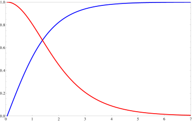
Figure 1: Numerical solution of the Nielsen-Olesen vortex: $X_{0}$ (blue) and $P_{0}$ (red). Notice $P_{0}$ falls off a little more slowly on this scale.

For later convenience, we give a lightning (but useful) review of the gravitational effect of this vortex. The idea here is to solve the Einstein equations,

$$R_{\mu\nu}-\frac{1}{2}Rg_{\mu\nu}=8\pi GT_{\mu\nu}\,,$$ (8)

simultaneously to the curved space abelian-Higgs vortex equations. The gravitational effect of the vortex is determined by the dimensionless ratio

$$\epsilon=8\pi G\eta^{2}\,,$$ (9)

which will typically be of order $10^{-7}-10^{-12}$ for cosmic strings of cosmological relevance. Thus, we can perform an expansion in $\epsilon$, finding the background (flat space) Nielsen-Olesen solution, and using its energy momentum to compute the leading order gravitational correction to flat space.

Looking for a static solution, we can choose a gauge in which the metric takes the form:

$$ds^{2}=e^{2\lambda}dt^{2}-e^{2(\nu-\lambda)}[dz^{2}+dR^{2}]-\alpha^{2}e^{-2\lambda}d\phi^{2}\,,$$ (10)

with curvature:

$$\sqrt{g}(R^{\phi}_{\phi}+R^{t}_{t}) = \alpha^{\prime\prime}\,,$$ (11)

$$\sqrt{g}R^{t}_{t} = [\alpha\lambda^{\prime}]^{\prime}\,,$$ (12)

$$\sqrt{g}R^{z}_{z} = [\alpha(\nu-\lambda)^{\prime}]^{\prime}\,,$$ (13)

$$\sqrt{g}R^{R}_{R} = \alpha^{\prime\prime}+\alpha(\nu^{\prime\prime}-\lambda^{\prime\prime})-\alpha^{\prime}(\lambda^{\prime}+\nu^{\prime})+2\alpha\lambda^{\prime 2}\,,$$ (14)

where $\alpha=R$, $\lambda=\nu=0$ to leading order.

The energy-momentum tensor of the vortex can readily be computed to leading order as:

$$T^{t}_{t}=T^{z}_{z}={\cal E} =X^{\prime 2}+\frac{X^{2}P^{2}}{R^{2}}+\beta\frac{P^{\prime 2}}{R^{2}}+\frac{1}{4}(X^{2}-1)^{2}\,,$$ (15)

$$T^{R}_{R}=-{\cal P}_{R} =-X^{\prime 2}+\frac{X^{2}P^{2}}{R^{2}}-\beta\frac{P^{\prime 2}}{R^{2}}+\frac{1}{4}(X^{2}-1)^{2}\,,$$

$$T^{\phi}_{\phi}=-{\cal P}_{\phi} =X^{\prime 2}-\frac{X^{2}P^{2}}{R^{2}}-\beta\frac{P^{\prime 2}}{R^{2}}+\frac{1}{4}(X^{2}-1)^{2}\,,$$

and a useful identity from the equations of motion (7) is

$$\frac{d~{}}{dR}[R{\cal P}_{R}]={\cal P}_{\phi}\,.$$ (16)

Solving the Einstein equations to leading order with this energy momentum tensor is then straightforward, and gives

$$\alpha = \left[1-\epsilon\int_{0}^{R}R({\cal E}-{\cal P}_{R})dR\right]R+\epsilon\int_{0}^{R}R^{2}({\cal E}-{\cal P}_{R})dR\,,$$ (17)

$$2\lambda = \epsilon\int_{0}^{R}R{\cal P}_{R}dR=\nu\,.$$ (18)

It is then easy to see the conical nature of this spacetime, as the exponential fall off of the $X$ and $P$ fields mean that the integrals converge rapidly, and the asymptotic form of the metric is

$$ds^{2}=d{\hat{t}}^{2}-d{\hat{z}}^{2}-d{\hat{R}}^{2}-{\hat{R}}^{2}(1-\epsilon{\hat{\mu}})^{2}d\phi^{2}\,,$$ (19)

where the coordinates have been rescaled (${\hat{t}}=e^{\epsilon\lambda_{\infty}}t$ etc.) to those of an asymptotic observer, and

$${\hat{\mu}}=1-\frac{d~{}}{dR}\alpha_{\infty}+2\lambda_{\infty}=\int_{0}^{\infty}R\,{\cal E}dR$$ (20)

is the renormalised energy per unit length of the cosmic string. Note that the effect of the transverse stresses of the string is to alter the details of the metric response, but that these details cancel out to leave the headline result that the conical deficit depends only on the energy per unit length of the string. For the Bogomolnyi limit $\beta=1={\hat{\mu}}$, these stresses vanish, and the string geometry is flat in the parallel ($t,z$) directions, and a smooth snub-nosed cone in the transverse ($R,\phi$) directions.

2.2 Cosmic string and Schwarzschild black hole

The basic idea of putting the vortex on the black hole is to first find an approximate solution assuming the string is much thinner than the horizon. There are (strictly speaking) three length scales, the two string core widths as already mentioned, and the black hole scale, however, by fixing the Bogomolnyi parameter and setting our scale to the string width, only one dimensionless parameter remains relevant: the black hole horizon radius, $r_{+}$, in units of string width (or $2GM\sqrt{\lambda}\eta$).

One then writes the vortex equations in the background of the Schwarzschild black hole:

$$-\Bigl{(}1\!-\!\frac{r_{+}}{r}\Bigr{)}X_{,rr}-\frac{2r\!-\!r_{+}}{r^{2}}X_{,r}-\frac{X_{,\theta\theta}}{r^{2}}-\frac{\cot\theta X_{,\theta}}{r^{2}}\!+\!\frac{1}{2}X(X^{2}\!-\!1)+\frac{XP^{2}_{\phi}}{r^{2}\sin^{2}\!\theta} = 0\,,\qquad$$ (21)

$$\left(1\!-\!\frac{r_{+}}{r}\right)\partial_{r}\partial_{r}P_{\phi}+\frac{1}{r^{2}}\partial_{\theta}\partial_{\theta}P_{\phi}+\frac{r_{+}}{r^{2}}\partial_{r}P_{\phi}-\frac{\cot\theta}{r^{2}}\partial_{\theta}P_{\phi}-\frac{X^{2}P_{\phi}}{\beta} = 0\,,\qquad\ \$$ (22)

and solves numerically. As noted in [3], for large $r_{+}$, these equations have a very good approximate solution of the form

$$X\simeq X_{0}(r\sin\theta)\,,\quad P_{\phi}\simeq P_{0}(r\sin\theta)\,.$$ (23)

Both this approximate solution, and the numerical integration, show that the vortex core is surprisingly undisturbed by the black hole, and the flux lines appear to simply “go through” the black hole (see figure 2).

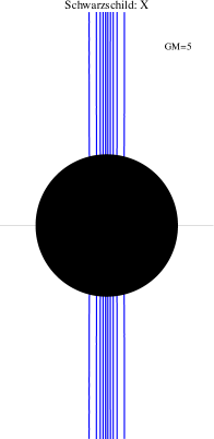
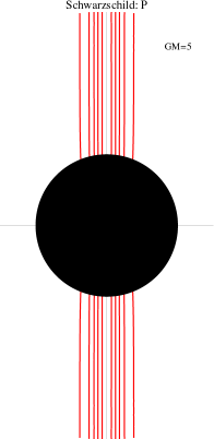
Figure 2: The equipotentials of the NO vortex in the Schwarzschild background. The Higgs contours are in blue, and the $P_{\phi}$ contours are in red. In each case contours are shown for $X,P_{\phi}=0.1,0.3,0.5,0.7,0.9$.

2.3 Flux expulsion: extremal RN black hole

When a small electric charge is added to the black hole the metric becomes the Reissner-Nordstrom (RN) solution, and there is no qualitative difference in how the string pierces the black hole, with ansatz (23) remaining a very good approximation to the exact solution for large RN black holes. However, when the black hole becomes extremal a new interesting phenomenon occurs: whereas for large extremal RN black holes the string still threads the horizon, below a certain critical mass, or black hole radius $r_{c}$, both the Higgs and the $U(1)$ fields are expelled from the black hole. The reason for this behavior is that in the extremal case, the horizon equations actually decouple from the exterior geometry [23] and admit a flux expulsion solution. In fact, the authors of [23] were able to place analytic bounds and demonstrate that for $r_{+}<0.7$ the expulsion must occur whereas for $r_{+}>2.9$ the penetration is inevitable. Numerical work actually places this threshold at about $r_{c}\approx 1.9$.

Since the discussion of this interesting behaviour is in some sense analogous to what we shall see in the extremal Kerr case let us recapitulate some of the features of this calculation. The vortex field equations in the RN background read

$$-\frac{1}{r^{2}}\partial_{r}(\Delta X_{,r})-\frac{1}{r^{2}\sin\theta}\partial_{\theta}(\sin\theta X_{,\theta})+\frac{XP_{\phi}^{2}}{r^{2}\sin^{2}\!\theta}-\frac{1}{2}X(1-X^{2}) = 0\,,$$ (24)

$$\partial_{r}\left(\frac{\Delta}{r^{2}}\partial_{r}P_{\phi}\right)+\frac{\sin\theta}{r^{2}}\partial_{\theta}\left(\frac{\partial_{\theta}P_{\phi}}{\sin\theta}\right)-\frac{X^{2}P_{\phi}}{\beta} = 0\,,$$ (25)

where $\Delta=r^{2}-2GMr+GQ^{2}=r^{2}g_{tt}$. Expanding near the horizon in the extremal case, when the metric function $\Delta$ has a double root $\Delta=(r-r_{+})^{2}$,

$$X=\xi_{0}(\theta)+(r-r_{+})\xi_{1}(\theta)+\dots\,,\quad P_{\phi}=\pi_{0}(\theta)+(r-r_{+})\pi_{1}(\theta)+\dots\,,$$ (26)

the horizon equations decouple from the exterior geometry, giving

$$\xi_{0}^{\prime\prime}+\cot\theta\xi_{0}^{\prime}-\frac{\xi_{0}\pi_{0}^{2}}{\sin^{2}\!\theta}+\frac{r_{+}^{2}}{2}\xi_{0}(1-\xi_{0}^{2}) =0\,,$$ (27)

$$\pi_{0}^{\prime\prime}-\cot\theta\pi_{0}^{\prime}-\frac{r_{+}^{2}}{\beta}\xi_{0}^{2}\pi_{0} =0\,,$$

where $\xi_{0}$ and $\pi_{0}$ must be symmetric around $\theta=\pi/2$, and obey $\xi_{0}=0,\pi_{0}=1$ at $\theta=0,\pi$. Obviously, such equations admit the flux expulsion solution $\xi_{0}=0,\pi_{0}=1$ everywhere. However, such a solution must extend to the bulk, which, as we shall see, is possible only for $r_{+}<r_{c}$.

To see this, suppose that expulsion occurs, i.e. on the horizon $X\equiv 0$, $P_{\phi}\equiv 1$, with $X$ increasing and $P_{\phi}$ decreasing towards their asymptotic values away from the horizon. Now consider a region close to the horizon in which $\partial_{r}(\Delta X_{,r})>0$ and $X^{2}\ll 1$, then from (24)

$$X>XP^{2}_{\phi}>\sin\theta\partial_{\theta}(\sin\theta X_{,\theta})+\frac{1}{2}{r_{+}^{2}}\sin^{2}\!\theta X\,.$$ (28)

Since $\sin\theta X_{,\theta}=0$ at $\theta=0,\pi/2$, and is positive for small $\theta$, its derivative must have at least one zero on $(0,\pi/2)$, so define $\theta_{0}<\pi/2$ as the first value of $\theta$ at which $\partial_{\theta}(\sin\theta X_{,\theta})=0$. From (28), $\frac{1}{2}r_{+}^{2}\sin^{2}\!\theta_{0}<1$, which is manifestly true for $r_{+}<\sqrt{2}$ so let us consider a larger black hole with $r_{+}>\sqrt{2}$, and define $\alpha>\theta_{0}$ by $r_{+}^{2}\sin^{2}\!\alpha=2$. Then, integrating (28) on the range $(\theta,\pi/2)$, for $\theta>\alpha$ gives

$$X_{,\theta}>\frac{1}{\sin\theta}\int_{\theta}^{\pi/2}\!\!\!\!d\theta^{\prime}X(\theta^{\prime})\left(\frac{r_{+}^{2}}{2}\sin\theta-\frac{1}{\sin\theta}\right)>\frac{X(\theta)}{\sin\theta}\int_{\theta}^{\pi/2}\!\!\!\!d\theta^{\prime}\left(\frac{r_{+}^{2}}{2}\sin\theta-\frac{1}{\sin\theta}\right)\,,$$

i.e.,

$$X_{,\theta}(\theta)>X(\theta)\left[\frac{r_{+}^{2}}{2}\cot\theta+\frac{\ln\tan(\theta/2)}{\sin\theta}\right]\,.$$ (29)

Due to the fact that $X_{,\theta\theta}<0$ on $[\theta_{0},\pi/2]$ and $X_{,\theta}(\theta)<\frac{X(\theta)-X(\alpha)}{\theta-\alpha}<\frac{X(\theta)}{\theta-\alpha}$, for consistency we must have

$$1>(\theta-\alpha)\left[\frac{\cot\theta}{\sin^{2}\!\alpha}+\frac{\ln\tan(\theta/2)}{\sin\theta}\right]$$ (30)

over the range $\theta\in(\alpha,\pi/2)$. One finds this is violated for $r_{+}^{2}>8.5$. Hence for $r_{+}\geq\sqrt{8.5}\approx 2.92$ the vortex must pierce the horizon.

A lower bound for $r_{c}$ can be obtained by considering the horizon equations (27). Namely, let a piercing solution of these equations exist. The second equation implies that $\pi_{0}$ monotonically decreases and reaches its first minimum $\pi_{m}\geq 0$ at $\theta=\pi/2$. Let us further assume that $\xi_{0}$ monotonically increases and reaches its first maximum $\xi_{M}\leq 1$ at $\theta=\pi/2$. Then one can derive, [23], that $r_{c}^{5}/(\sqrt{2}-r_{c})^{2}\geq\beta^{2}/\sqrt{2}$, giving $r_{c}\simeq 0.7$ for $\beta=1$.

Numerical work shows that (taking $\beta=1$) a transition between the penetration and expulsion actually occurs for $r_{c}\approx 1.9$, in which case $\pi_{m}\approx 1$ and $\xi_{M}\approx 0$. Such a transition is therefore continuous from the point of view of the fields on the horizon. The RN flux expulsion phase transition is indicated in figure 5, where it is compared to the Kerr case. It is worth remarking on the response of this phase transition to the Bogomolnyi parameter, $\beta$. As $\beta$ drops, the gauge core becomes more confined, and thus we see a drop in the critical mass before the black hole becomes small enough to sit inside the magnetic flux core. On the other hand, for $\beta\geq{\cal O}(1)$, the gauge core is more diffuse, leading to a behaviour in the Higgs field more analogous to a global vortex. The order parameter (the value of the Higgs field at $\theta=\pi/2$) drops more smoothly, before finally the flux expulsion kicks in when the black hole finally comes within the Higgs core, at roughly the same critical mass as for a $\beta=1$ vortex. We shall see that all these features (continuity, $\beta$-dependence) are substantially different for the extremal Kerr black hole.

3 Higgs hair for the Kerr black hole

3.1 Approximate solution

The Kerr geometry [in $(+,-,-,-)$ signature] reads

$$ds^{2}=\frac{\Delta\!-\!a^{2}\sin^{2}\!\theta}{\Sigma}dt^{2}+\frac{4GMar\sin^{2}\!\theta}{\Sigma}dtd\varphi\!-\!\Sigma d\theta^{2}-\frac{\Gamma}{\Sigma}\sin^{2}\!\theta\,d\varphi^{2}\!-\!\frac{\Sigma}{\Delta}dr^{2}\,,\quad\$$ (31)

where $a=J/M$ and

$$\Sigma=r^{2}+a^{2}\cos^{2}\!\theta\,,\quad\Delta=r^{2}-2GMr+a^{2}\,\qquad\Gamma=(r^{2}+a^{2})^{2}-\Delta a^{2}\sin^{2}\theta\,.$$ (32)

Due to the rotation, we expect a mixing between the $t$ and $\phi$ degrees of freedom, so we consider both a nonzero $P_{\phi}$ and $P_{t}$:

$$\frac{X^{2}}{\beta}P_{\phi} = \frac{\Delta}{\Sigma}\partial_{r}\partial_{r}P_{\phi}+\frac{1}{\Sigma}\partial_{\theta}\partial_{\theta}P_{\phi}+\frac{2GM\rho^{2}}{\Sigma^{3}}(r^{2}-a^{2}\cos^{2}\!\theta)\partial_{r}P_{\phi}$$

$$-\frac{\cot\theta}{\Sigma^{3}}(\Sigma^{2}+4GMra^{2}\sin^{2}\!\theta)\partial_{\theta}P_{\phi}-\frac{4a^{3}GMr}{\Sigma^{3}}\cos\theta\sin^{3}\!\theta\partial_{\theta}P_{t}$$

$$+\frac{2GMa\sin^{2}\!\theta}{\Sigma^{3}}\bigl{[}2r^{2}\Sigma+\rho^{2}(r^{2}-a^{2}\cos^{2}\!\theta)\bigr{]}\partial_{r}P_{t}\,,$$

$$\frac{X^{2}}{\beta}P_{t} = \frac{\triangle}{\Sigma}\partial_{r}\partial_{r}P_{t}+\frac{1}{\Sigma}\partial_{\theta}\partial_{\theta}P_{t}+\frac{4GMra}{\Sigma^{3}}\cot\theta\left(\partial_{\theta}P_{\phi}+a\sin^{2}\!\theta\partial_{\theta}P_{t}\right)+\frac{\cot\theta}{\Sigma}\partial_{\theta}P_{t}$$ (34)

$$+\frac{2GMa}{\Sigma^{3}}(\Sigma-2r^{2})\partial_{r}P_{\phi}-\frac{1}{\Sigma^{3}}\bigl{[}2GM(2r^{2}\rho^{2}-a^{2}\sin^{2}\!\theta\Sigma)-2r\Sigma^{2}\bigr{]}\partial_{r}P_{t}\,,\qquad\qquad$$

$$0 = \frac{\Delta}{\Sigma}X_{,rr}+\frac{2(r-GM)}{\Sigma}X_{,r}+\frac{X_{,\theta\theta}}{\Sigma}+\frac{\cot\theta X_{,\theta}}{\Sigma}+\frac{1}{2}X(1-X^{2})+XP_{\mu}^{2}\,,\qquad$$ (35)

where $\rho^{2}=r^{2}+a^{2}$ has been introduced for visual clarity, and

$$P_{\mu}^{2}=\frac{(\rho^{2}P_{t}+aP_{\phi})^{2}}{\Sigma\Delta}-\frac{(P_{\phi}+a\sin^{2}\!\theta P_{t})^{2}}{\Sigma\sin^{2}\!\theta}\,.$$ (36)

We now see explicitly why we needed to introduce the $P_{t}$ field (indeed, this was first noted by Wald [30] who found an expression for constant probe magnetic flux field through a Kerr black hole). Clearly (34) does not allow $P_{t}=0$ unless $a=0$. Indeed, a little investigation shows that the approximate analytic solution (23) can be generalized in the Kerr case to

$$X\simeq X_{0}(R)\,,\quad P_{\phi}\simeq P_{0}(R)\,,\quad P_{t}\simeq-\frac{2GMar}{\rho^{4}}P_{0}(R)\,,\quad R\equiv\rho\sin\theta.$$ (37)

Figure 3 illustrates how good an approximation to the full numerical solution this expression is.

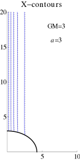
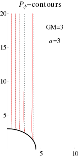
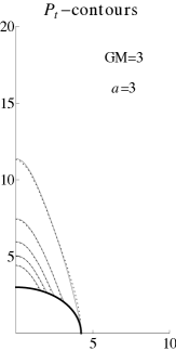
Figure 3: A comparison of the approximate and exact numerical solutions for an extremal $GM=a=3$ Kerr black hole. In spite of the low value of black hole mass, (37) is still an extremely good approximation to the actual result. Here, the Higgs contours are in blue, the $P_{\varphi}$ contours in red, the $P_{t}$ contours in grey, and all the corresponding approximate solution contours in dashed black. Contours are shown for $X,P_{\varphi}=0.1,0.3,0.5,0.7,0.9$, and for $P_{t}=-0.099,-0.077,-0.055,-0.033,-0.011$.

3.2 Numerical solution

In order to demonstrate conclusively that the abelian Higgs vortex is compatible with the rotating black hole, we need to numerically integrate the equations of motion. Since this is an elliptic problem we used a gradient flow method on a polar grid, updating the event horizon as per the method of [3] with the constraint that on the horizon

$$P_{t}=-\frac{aP_{\phi}}{r_{+}^{2}+a^{2}}\,.$$ (38)

For the Kerr black hole however, there is also an additional subtlety: the vortex boundary conditions ($X=0$, $P_{\varphi}=1$) placed on axis only restrict the $X$ and $P_{\varphi}$ fields, and not $P_{t}$. This is not surprising and represents the fact that there is a dyonic degree of freedom the black hole introduces to the solution. (This also exists in the Schwarzschild set-up, but was not noticed as the electric and magnetic degrees of freedom of the gauge boson decouple there.) Since we do not wish to pick up a spurious charge of the black hole, we allow the $P_{t}$ field to relax freely, and update it along the axis by continuity, thus ensuring that $P_{t}$ is only as big as it needs to be to counter the magnetic part of the vortex. Figure 4 shows some sample solutions for a large-ish black hole both at, and away from, extremality.

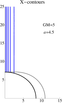
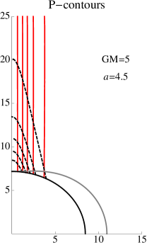
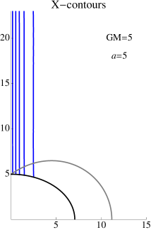
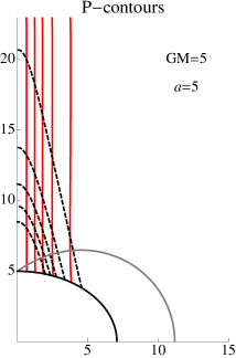
Figure 4: Numerical solution for a Kerr black hole with the values of $GM$ and $a$ indicated. On the left, the $X=0.1,0.3,0.5,0.7,0.9$ contours are plotted in blue. On the right, the $P_{\varphi}=0.1,0.3,0.5,0.7,0.9$ contours are in red, and the $P_{t}=-0.045,-0.035,-0.025,-0.015,-0.005$ contours are in dashed black. The horizon is shown in black, and the edge of the ergosphere in grey.

4 Extremal Kerr black holes

Having shown that the vortex can sit through a black hole, at the price of some induced electric field, it is interesting to look at the extremal limit of the Kerr black hole in more detail. As we have seen in Sec. 2.3, for the RN black hole, a phenomenon of flux expulsion was observed for small enough black holes; essentially the event horizon is an infinite proper distance away, and provided the overall radius of the black hole sits roughly in the core of the string, it is easier for the magnetic flux lines of the massless vector field in the core to avoid the black hole than pierce it – it is only once the boson becomes massive outside the string core that the energy scales tip the other way. Thus, do we get the same phenomenon here? There is reason to believe we should. In an elegant construction, Wald, [30], showed how Killing fields generate probe electromagnetic fields on Ricci flat backgrounds, and presented a particular solution which represents a constant axial magnetic field threading the black hole. The gauge potential has the form

$$A^{\mu}\propto\left(2a\partial_{t}+\partial_{\varphi}\right)^{\mu}\,,$$ (39)

which generates a uniform magnetic field $B_{z}$ far from the black hole, and has zero nett charge on the black hole. The electric field is not however vanishing, and instead sweeps down the axes and out along the equator. While the flux lines of the Wald solution cross the horizon for nonextremal black holes, for all extremal black holes, the flux is expelled.

Clearly the Wald solution only works for a massless vector field, however, one could argue that for small black holes which are well below the scale of the string, the black hole will be sitting in the string core, and should therefore see the gauge field as effectively massless and hence repel it giving rise to flux expulsion. To some extent this interpretation is correct, however, the situation is a great deal more complex. In the Wald solution, the photon is massless throughout the whole of spacetime, whereas for the string, the gauge field is only approximately massless inside the string core. Thus the Wald electric flux, which sweeps down from the poles and out at the equator, now cannot correspond to an electrically neutral black hole inside the string core. We therefore cannot simply use the Wald expression as an approximate core solution. Nonetheless, we find a similar expulsion phenomenon occurs, although the numerical sensitivity of the low mass black hole system leads us to suspect that there is a dynamical instability in the small extremal black hole, analogous to the Kerr-adS instability [27]. It is interesting that extremal Kerr is so different from extremal RN, however, perhaps not surprising due to the rather different structure of the near horizon spacetime.

4.1 Near horizon expansion

To study the near horizon limit, it is useful to rewrite the vector field in terms of the alternative variables $P$ and $Q$:

$$P =P_{\varphi}+a\sin^{2}\!\theta P_{t}\,,$$ (40)

$$Q =\rho^{2}P_{t}+aP_{\varphi}\,,$$

giving

$$\Bigl{[}\frac{P^{2}}{\Sigma\sin^{2}\!\theta}\!\! - \!\!\frac{Q^{2}}{\Sigma\Delta}\Bigr{]}X=\frac{\Delta}{\Sigma}X_{,rr}+\frac{2(r-GM)}{\Sigma}X_{,r}+\frac{X_{,\theta\theta}}{\Sigma}+\frac{\cot\theta X_{,\theta}}{\Sigma}+\frac{1}{2}X(1-X^{2})\,,\qquad\quad$$ (41)

$$\frac{X^{2}P}{\beta} = \frac{\Delta}{\Sigma}P_{,rr}+\frac{P_{,\theta\theta}}{\Sigma}-\frac{\cot\theta P_{,\theta}}{\Sigma}\Bigl{(}1-\frac{2a^{2}\sin^{2}\!\theta}{\Sigma}\Bigr{)}+\frac{2P_{,r}}{\Sigma^{2}}\bigl{[}\Sigma(r-GM)-r\Delta\bigr{]}$$ (42)

$$+\frac{2a\sin^{2}\!\theta}{\Sigma^{2}}\Bigl{(}rQ_{,r}-\cot\theta Q_{,\theta}+aP-Q\Bigr{)}\,,$$

$$\frac{X^{2}Q}{\beta} = \frac{\Delta}{\Sigma}Q_{,rr}+\frac{Q_{,\theta\theta}}{\Sigma}-\frac{\cot\theta Q_{,\theta}}{\Sigma}\Bigl{(}1-\frac{4GMr}{\Sigma}\Bigr{)}$$ (43)

$$+\frac{2\Delta}{\Sigma^{2}}\bigl{[}\cot\theta(Q_{,\theta}-aP_{,\theta})-r(Q_{,r}-aP_{,r})+Q-aP\bigr{]}\,.$$

In particular, for the extremal Kerr black hole $\Delta=(r-r_{+})^{2}$ and so, similar to the RN case, we expand near the horizon

$$X = \xi_{0}(\theta)+(r-r_{+})\xi_{1}(\theta)+\dots\,,$$

$$P = \pi_{0}(\theta)+(r-r_{+})\pi_{1}(\theta)+\dots\,,$$ (44)

$$Q = \psi_{0}(\theta)+(r-r_{+})\psi_{1}(\theta)+\dots\,.$$

Eq. (41) (or finiteness of energy on horizon) then implies that $\psi_{0}=0$, and the leading order pieces of each equation read

$$\xi_{0}^{\prime\prime}+\cot\theta\xi_{0}^{\prime}+\frac{r_{+}^{2}}{2}(1+\cos^{2}\!\theta)\xi_{0}(1-\xi_{0}^{2})-\Bigl{[}\frac{\pi_{0}^{2}}{\sin^{2}\!\theta}-\psi_{1}^{2}\Bigr{]}\xi_{0} = 0\,,$$ (45)

$$\pi_{0}^{\prime\prime}-\cot\theta\frac{3\cos^{2}\!\theta-1}{1+\cos^{2}\!\theta}\pi_{0}^{\prime}+\frac{2\sin^{2}\!\theta}{1+\cos^{2}\!\theta}(\psi_{1}+\pi_{0})-\frac{r_{+}^{2}}{\beta}\xi_{0}^{2}\pi_{0}(1+\cos^{2}\!\theta) = 0\,,$$ (46)

$$\psi_{1}^{\prime\prime}+\cot\theta\frac{3-\cos^{2}\!\theta}{1+\cos^{2}\!\theta}\psi_{1}^{\prime}-\frac{r_{+}^{2}}{\beta}\xi_{0}^{2}\psi_{1}(1+\cos^{2}\!\theta) = 0\,.\qquad\quad$$ (47)

Note that although the expansion does not in general decouple from the bulk (because of the appearance of $\psi_{1}$) it does form a closed system in this extremal case. The constraints on the solutions are that they must be symmetric around $\theta=\pi/2$, and $\xi_{0}=0$, $\pi_{0}=1$ at $\theta=0,\pi$.

4.2 Flux penetration and expulsion

Let us first show that for large black holes a string will always penetrate the black hole horizon. Similar to the extremal RN case, we proceed by contradiction. Returning to the full bulk equation (41), let us assume that flux expulsion occurs, i.e. at $r_{+}=a=GM$ we have $X=0$ and $P_{\varphi}=1$ (with $P_{t}=-1/2r_{+}$) leading to $P=(1+\cos^{2}\theta)/2$, and hence $Q^{\prime}(r_{+})=-1$ from (46). Therefore near $r_{+}$ both $\partial_{r}(\Delta\partial_{r}X)>0$, and $(Q^{2}/\Delta\Sigma-X^{2}/2)>0$. Hence Eq. (41) implies

$$\frac{1}{2}r_{+}^{2}\sin^{2}\!\theta X\! + \!\sin\theta\partial_{\theta}(\sin\theta\partial_{\theta}X)$$ (48)

$$\leq \frac{1}{2}r_{+}^{2}(1+\cos^{2}\!\theta)\sin^{2}\!\theta X+\sin\theta\partial_{\theta}(\sin\theta\partial_{\theta}X)<XP^{2}<X\,.\qquad\$$

However, this is the same equation (28) as discussed in Sec. 2.3 and the discussion therein therefore applies. Hence we conclude that for any $r_{+}>\sqrt{8.5}\approx 2.92$ the vortex must pierce the extremal Kerr black hole.

Let us now look more closely at what happens on the horizon. A simple inspection of (47) shows that if $\xi_{0}\neq 0$, then $\psi_{1}=0$. Eqs. (45) and (46) now read

$$\xi_{0}^{\prime\prime}+\cot\theta\xi_{0}^{\prime}+\frac{r_{+}^{2}}{2}(1+\cos^{2}\!\theta)\xi_{0}(1-\xi_{0}^{2})-\frac{\pi_{0}^{2}\xi_{0}}{\sin^{2}\!\theta} =0\,,$$ (49)

$$\pi_{0}^{\prime\prime}-\cot\theta\frac{3\cos^{2}\!\theta-1}{1+\cos^{2}\!\theta}\pi_{0}^{\prime}+\frac{2\sin^{2}\!\theta}{1+\cos^{2}\!\theta}\pi_{0}-\frac{r_{+}^{2}}{\beta}\xi_{0}^{2}\pi_{0}(1+\cos^{2}\!\theta) =0\,,$$

and form a pair of equations purely representing data on the horizon, decoupled from the bulk. A general analytic discussion of these equations is rather involved. However, let us assume, based on energetic considerations – similar to the extremal RN case, that the fields $\xi_{0}$ and $\pi_{0}$ have only one turning point on the horizon (a fact confirmed to a certain extent by a numerical analysis). Then the field $\xi_{0}$ starts from zero at $\theta=0$ and monotonically increases to reach its first maximum at $\theta=\pi/2$, $\xi_{M}=\xi_{0}(\pi/2)<1$, while the value of $\pi_{0}$ monotonically decreases to reach its first minimum $\pi_{m}=\pi_{0}(\pi/2)<1$. Since $\pi_{0}^{\prime\prime}(\pi/2)>0$, the second equation at $\theta=\pi/2$ implies that $r_{+}^{2}\xi_{M}^{2}-2\beta>0$, i.e., $r_{+}^{2}>2\beta$. Thus, for $r_{+}<\sqrt{2\beta}$ the penetrating solution cannot exist and expulsion must occur.

To show that the flux expulsion is indeed a solution of our near horizon equations (45)–(47) we now consider the case when $\xi_{0}\equiv 0$. Then $\psi_{1}={const.}$, and (46) has the general solution $\pi_{0}=\lambda\sin^{2}\!\theta+\gamma\cos\theta-\psi_{1}$. Applying the boundary conditions, and symmetry around $\pi/2$, then yields $\gamma=0$, $\psi_{1}=-1$. Moreover, the requirement that the field strength invariant $F_{\mu\nu}F^{\mu\nu}$ remains finite at $\theta=0$ implies $\lambda=-1/2$. Therefore the solution reads $\pi_{0}=-\frac{1}{2}\sin^{2}\!\theta+1$ and $\psi_{0}=0$. In the original variables this corresponds to

$$P_{\phi} = 1\,,\qquad P_{t}=-\frac{1}{2r_{+}}\,,$$ (50)

on the horizon and hence represents a flux-expelled solution. Let us remark that if there is a phase transition between the flux penetration and expulsion, the value of $\psi_{1}$ on the horizon necessarily suffers from a discontinuity: $\psi_{1}=0$ for flux penetration whereas $\psi_{1}=-1$ in the case of expulsion.

Our analytic arguments suggest that similar to the RN case there exists a critical radius $r_{c}$, $1.41<r_{c}<2.92$ for $\beta=1$, below which the flux is necessarily expelled. Numerical investigations actually indicate $r_{c}\approx 1.912$. The situation seems, however, slightly different to the RN case. Whereas we have seen that for the extremal RN black holes the transition was continuous (the fields on the horizon vary smoothly between the penetrating and the expelling phase), in the case of the extremal Kerr black hole we find a very sharp transition. For example, for $\beta=1$, we find that for $r_{+}=1.911855$ a piercing solution of Eqs. (49) exists with $\pi_{m}\approx 0.57515$ and $\xi_{M}\approx 0.76166$ whereas there is no piercing solution for $r_{+}=1.9118525$. The phase transition would appear to be discontinuous. This is backed up by the fact that the first derivative of the $Q$-field, $\psi_{1}$, is discontinuous between expulsion and penetration.

Figure 5 shows a comparison of the Kerr and RN phase transitions for several values of $\beta$. The order parameter plotted is the maximum value of the Higgs field, $X_{m}=\xi_{0}(\pi/2)$, attained on the equator. Interestingly, not only is the nature of the Kerr phase transition different from that of RN, but also the response to varying $\beta$ is quite different. While both exhibit a lowering of critical radius as $\beta$ drops (because of the gauge core becoming thinner), in contrast to the RN case the Kerr black hole has higher critical radius as $\beta$ increases. While in both instances for smaller $\beta$ the gauge core becomes more diffuse, the nature of the equations governing the gauge fields is different. For Kerr, it is the combination of $P_{\varphi}$ and $P_{t}$, $\pi_{0}$, that is determined on the horizon, and this has two contributions to its effective local mass in (49): One geometric, and one coming from the Higgs field, which must dominate if $\pi_{0}$ is not to expel. Once the flux expels, we require $\psi_{1}=-1$, and hence $\xi_{0}=0$. Since the term involving the Higgs field has a factor $r_{+}^{2}/\beta$, it is clear that increasing $\beta$ will increase the critical expulsion radius. We believe that this interesting behavior deserves more attention in the future.

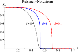
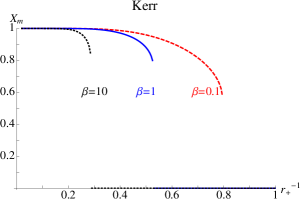
Figure 5: Phase plots for the RN and Kerr extremal black holes. The maximum value of the Higgs field, $X_{m}=\xi_{0}(\pi/2)$, is plotted against the horizon radius $r_{+}$. The transition is shown for different values of the Bogomolnyi parameter: $\beta=10$ in dotted black, $\beta=1$ in solid blue, and $\beta=0.1$ in dashed red.

5 Backreaction of the vortex on the black hole

In the literature, it has been assumed (see e.g. [25, 31]) that the geometry of a cosmic string threading a Kerr black hole will simply be given by the Kerr solution with the $\varphi-$angle having a reduced range corresponding to the angular deficit. However, here we will show that this is not in fact the case. The situation is more subtle, and far more interesting. In brief, what we show is that the string does indeed induce a conical deficit, but a deficit from the perspective of an azimuthal coordinate co-rotating with the black hole, so that the event horizon of the black hole is a 2-sphere with a wedge removed. Because the horizon is rotating relative to an asymptotic observer, this is not equivalent to a simple angular deficit in the full spacetime, but rather, there is a more complex response in the region of the black hole, with the asymptotic deficit angle behaviour recovered only at large $r$. As a consequence, the ergosphere is shifted, and nearby orbits of Kerr black holes will also be affected.

Our approach is to use the perturbative technique of [3, 13], in which we solve the full Einstein-abelian Higgs system order by order in $\epsilon=8\pi G\eta^{2}$. Strictly, as we wish to present simple ‘analytic’ expressions, we also solve for a “thin” string, in which $\sqrt{\lambda}\eta r_{+}\gg 1$. For small $\epsilon$, we can use the probe vortex solution to compute the leading order gravitational backreaction, and for large black holes, we have demonstrated that our ‘analytic’ approximation (37) is an excellent expression which closely mimics the full numerical solution. In particular, it is a reliable expression both within the core of the string, and on the horizon of the black hole.

In order to proceed, we need to express the metric in a useful set of coordinates which reflect the axial symmetry of the Kerr-cosmic string set-up. For this purpose we shall use the Weyl form of the metric (see e.g. [32])

$$ds^{2}=e^{2\lambda}dt^{2}-\alpha^{2}e^{-2\lambda}\bigl{[}d\varphi+Bdt\bigr{]}^{2}-e^{2(\nu-\lambda)}(dx^{2}+dy^{2})\,,$$ (51)

where the functions $\alpha,B,\nu$ and $\lambda$ are functions of the $x$ and $y$ coordinates only. Note the similarity with (10), only there the functions depended only on one coordinate. The Ricci tensor of this metric is given by:

$$R^{\varphi}_{\varphi}+R^{t}_{t} = e^{2(\lambda-\nu)}\frac{\nabla^{2}\alpha}{\alpha}\,,$$ (52)

$$R^{t}_{\varphi} = \frac{\alpha}{2}e^{-2(\lambda+\nu)}\Bigl{[}-3\nabla\alpha\cdot\nabla B+4\alpha\nabla B\cdot\nabla\lambda-\alpha\nabla^{2}B\Bigr{]}\,,$$ (53)

$$R_{\varphi\varphi} = -\frac{\alpha}{2}e^{-2\nu}\Bigl{[}\alpha^{3}e^{-4\lambda}(\nabla B)^{2}+2\nabla^{2}\alpha-2\nabla\alpha\cdot\nabla\lambda-2\alpha\nabla^{2}\lambda\Bigr{]}\,,$$ (54)

$$R^{x}_{x}+R^{y}_{y} = \frac{e^{2(\lambda-\nu)}}{2\alpha}\Bigl{[}2{\nabla^{2}\alpha}-{\alpha^{3}e^{-4\lambda}}(\nabla B)^{2}+4e^{\lambda}\nabla\cdot\left(\alpha\nabla e^{-\lambda}\right)+4\alpha\nabla^{2}\nu\Bigr{]}\,,$$ (55)

$$R_{xy} = \frac{1}{2\alpha}\bigl{[}\alpha^{3}e^{-4\lambda}B_{x}B_{y}-4\alpha\lambda_{x}\lambda_{y}+2(\alpha_{x}\nu_{y}+\alpha_{y}\nu_{x})-2\alpha_{xy}\Bigr{]}\,,$$ (56)

$$R_{y}^{y} = \frac{e^{2(\lambda-\nu)}}{2\alpha}\Bigl{[}-\alpha^{3}e^{-4\lambda}B_{y}^{2}+2\alpha\nabla^{2}(\nu-\lambda)-2(\alpha_{y}\nu_{y}-\alpha_{x}\nu_{x})$$ (57)

$$\qquad-2\nabla\alpha\cdot\nabla\lambda+4\alpha\lambda_{y}^{2}+2\alpha_{yy}\Bigr{]}\,,$$

where we have introduced the two-dimensional gradient operator $\nabla=(\partial_{x},\partial_{y})$ as well as the corresponding dot product, expressing for example the Laplace operator as $\nabla^{2}=\nabla\cdot\nabla=\partial_{x}^{2}+\partial_{y}^{2}$.

In particular, defining

$$x=\int\frac{dr}{\sqrt{\Delta}}\,,\quad y=\theta\,,$$ (58)

the background (Kerr) solution can be written as

$$\alpha_{0}=\sqrt{\Delta}\sin\theta\,,\quad B_{0}=-\frac{2aGMr}{\Gamma}\,,\quad e^{2\nu_{0}}=\frac{\Delta\Sigma^{2}}{\Gamma}\,,\quad e^{2\lambda_{0}}=\frac{\Delta\Sigma}{\Gamma}\,.$$ (59)

The procedure for finding the back-reacted vortex solution is to use the analytic approximation (37) to find the energy momentum of the vortex solution, which will be a good approximation to the true energy momentum, and to use this to find the leading order correction to the metric by expanding the Einstein equations,

$$R_{\mu\nu}=\epsilon\Bigl{(}T_{\mu\nu}-\frac{1}{2}Tg_{\mu\nu}\Bigr{)}\,,\quad\epsilon\equiv 8\pi G_{N}\eta^{2}\,,$$ (60)

around the background Kerr solution using the Weyl expressions (59).

In this limit, the energy momentum tensor is found to leading order to be

$$T^{t}_{t} \approx T^{x}_{x}\approx X_{0}^{\prime 2}+\frac{X_{0}^{2}P_{0}^{2}}{R^{2}}+\beta\frac{{P_{0}^{\prime}}^{2}}{R^{2}}+\frac{1}{4}(X_{0}^{2}-1)^{2}\equiv{\cal E}\,,$$ (61)

$$T^{y}_{y} \approx-X_{0}^{\prime 2}+\frac{X_{0}^{2}P_{0}^{2}}{R^{2}}-\beta\frac{P_{0}^{\prime 2}}{R^{2}}+\frac{1}{4}(X_{0}^{2}-1)^{2}\equiv-{\cal P}_{R}\,,$$

$$T^{\varphi}_{\varphi} \approx X_{0}^{\prime 2}-\frac{X_{0}^{2}P_{0}^{2}}{R^{2}}-\beta\frac{P_{0}^{\prime 2}}{R^{2}}+\frac{1}{4}(X_{0}^{2}-1)^{2}\equiv-{\cal P}_{\phi}\,,$$

$$T_{xy} \approx\frac{\sqrt{\Delta}r}{\rho}R({\cal E}+{\cal P}_{R})\,,$$

$$T^{t}_{\varphi} \approx-\frac{4GMra}{\rho^{8}}\left[(\rho^{2}-4r^{2})RPP^{\prime}-a^{2}R^{2}(X^{2}P^{2}+P^{\prime 2})\right]\approx 0\,,$$

where ${\cal E}$ etc. denote the energy-momentum components of the Nielsen-Olesen vortex, defined in (15), which are simply functions of $R=\rho\sin\theta$. Because these components are functions of the $R$ variable only, this leads to a modification of the Kerr geometry which is also dependent on $R$.

In order to motivate the form of the perturbed metric, we first note that at large “$r\cos\theta$”, the metric should approach the form of the isolated gravitating vortex, given in (17,18). Thus we expect that $\delta\alpha=\epsilon\alpha_{0}\alpha_{1}(R)$, $\delta\lambda=\delta\nu/2=\epsilon\lambda_{1}(R)$. Of course we must confirm that the equations of motion indeed lead to perturbations of this form.

First, consider the Einstein equation (52),

$$\delta(R^{t}_{t}+R^{\varphi}_{\varphi})=\frac{e^{2(\lambda-\nu)}}{\alpha}\nabla^{2}\delta\alpha=\frac{\nabla^{2}\delta\alpha}{\sqrt{\Delta}\rho R}=-\epsilon\,({\cal E}-{\cal P}_{R})\,,$$ (62)

which is solved to leading order by a perturbation of the form

$$\alpha=\alpha_{0}\Bigl{(}1+\epsilon\alpha_{1}(R)+O(\epsilon^{2})\Bigr{)}\,.$$ (63)

where $\alpha_{1}$ satisfies

$$\alpha_{1}^{\prime\prime}+2\frac{\alpha_{1}^{\prime}}{R}=-({\cal E}-{\cal P}_{R})\;\;\;\Rightarrow\;\;\;\alpha_{1}=-\int_{0}^{R}\!\!\!R({\cal E}-{\cal P}_{R})dR+\frac{1}{R}\int_{0}^{R}\!\!\!R^{2}({\cal E}-{\cal P}_{R})dR\,,$$ (64)

which is in fact identical in form to the self-gravitating correction (17).

Next, noting that $B$ and its derivatives are subdominant, we obtain for the next Einstein equations (54), (55) and (57)

$$\delta R_{\varphi\varphi} = -\epsilon R\left[R\alpha_{1}^{\prime\prime}+2\alpha_{1}^{\prime}-R\lambda_{1}^{\prime\prime}-\lambda_{1}^{\prime}\right]=R^{2}\left[{\cal E}+\frac{1}{2}({\cal P}_{\phi}-{\cal P}_{R})\right]\,,$$ (65)

$$\delta(R^{x}_{x}+R^{y}_{y}) = \epsilon\left[\alpha_{1}^{\prime\prime}+\frac{\alpha_{1}^{\prime}}{R}+2\nu_{1}^{\prime\prime}-2\lambda_{1}^{\prime\prime}-2\frac{\lambda_{1}^{\prime}}{R}\right]=-\epsilon\left[{\cal E}-{\cal P}_{\phi}\right]\,,$$ (66)

$$\delta R^{y}_{y} = \epsilon\left[\alpha_{1}^{\prime\prime}+\frac{\alpha_{1}^{\prime}}{R}+\nu_{1}^{\prime\prime}-\lambda_{1}^{\prime\prime}-\frac{\nu_{1}^{\prime}}{R}-\frac{\lambda_{1}^{\prime}}{R}\right]=-\epsilon\left[{\cal E}-\frac{1}{2}({\cal P}_{\phi}-{\cal P}_{R})\right]\,,\qquad$$ (67)

the first of which gives

$$\lambda_{1}=\frac{1}{2}\int_{0}^{R}R{\cal P}_{R}dR\,,$$ (68)

and consistency with the next two implies $\nu_{1}=2\lambda_{1}$, also as in the self-gravitating case.

Now we can examine the variation $\delta B$, which cannot be deduced from an asymptotic analysis, since the background function $B={\cal O}(r^{-3})$ is subdominant. Instead, we must examine the near horizon behaviour of (56), in which the only term not explicitly convergent is

$$\alpha_{0}^{2}e^{-4\lambda_{0}}B_{0,x}\delta B_{,y}\sim-\frac{2GMa}{\rho^{2}\sqrt{\Delta}}\left(1-\frac{4r^{2}}{\rho^{2}}\right)R^{2}\delta B_{,y}\,.$$ (69)

Given the RHS of this equation from (61), we quickly see that we cannot find a form of $\delta B$ which has the requisite functional dependence on the background coordinates, as well as on the variable $R$. In particular, it is transparent that if we set $\delta B=\epsilon B_{0}\alpha_{1}^{-1}$, which is what would be required for a pure $\varphi$-angular conical deficit, then this would lead to a divergence in $\delta R_{xy}$ at the horizon, and would not solve the Einstein equations. Thus $\delta B=0$. This simple result will have significant consequences as we will see.

We can now check the remaining equations:

$$\delta R_{xy} = -\epsilon\sqrt{\Delta}\;\frac{r}{\rho}\left[R\alpha_{1}^{\prime\prime}+2\alpha_{1}^{\prime}-4\lambda_{1}^{\prime}\right]=\epsilon\sqrt{\Delta}\;\frac{r}{\rho}\left[{\cal E}+{\cal P}_{R}\right]\,,$$ (70)

$$\delta R^{t}_{\varphi} = \epsilon\frac{GMra}{\rho^{8}}\left(\rho^{2}-4r^{2}+2a^{2}\right)R^{3}\left[3\alpha_{1}^{\prime}-4\lambda_{1}^{\prime}\right]$$

$$= -\epsilon\frac{4GMra}{\rho^{8}}\left[(\rho^{2}-4r^{2})RPP^{\prime}-a^{2}R^{2}(X^{2}P^{2}+P^{\prime 2})\right]={\cal O}(r_{+}^{2}/r^{5})\,.$$

Pulling all the details together, and looking outside the core of the vortex, we see the asymptotic form of the Kerr-vortex is

$$ds^{2}= \left(1-\frac{2GMr}{\Sigma}+\frac{8(GMar\sin\theta)^{2}}{\Gamma\Sigma}\epsilon{\hat{\mu}}\right)dt^{2}-\!\Sigma d\theta^{2}-\!\frac{\Sigma}{\Delta}dr^{2}$$ (72)

$$-\frac{\Gamma}{\Sigma}(1-2\epsilon{\hat{\mu}})\sin^{2}\!\theta\,d\varphi^{2}\!+\frac{4GMar\sin^{2}\!\theta}{\Sigma}(1-2\epsilon{\hat{\mu}})dtd\varphi\,,$$

where $\hat{\mu}$ is the renormalised energy per unit length of the string defined in (20). It is clear that while there is an angular deficit in this spacetime, which does approach the standard conical deficit at large distances, in the vicinity of the black hole, as far as these Boyer-Lindquist coordinates are concerned, the deficit is felt not only by the ‘angular’ $\varphi$-coordinate, but also by the time component of the metric. While this seems a little strange and worrying, if we instead transform to a frame co-rotating with the black hole, $\varphi_{H}=\varphi-\Omega_{H}t=\varphi-B(r_{+})$, then the effect of the cosmic string is indeed to remove a deficit angle – from the perspective of the black hole. Note this is not in contradiction with the Schwarzschild result, it is simply that in Schwarzschild there is no difference between the spatial angular variable on the horizon and that at infinity.

6 Discussion

To sum up: we have shown how to correctly thread a rotating black hole with vortex hair. A consequence of rotation is that the angular and time components of not only the metric, but also the vortex fields are interconnected. This leads to an electric field in the polar regions of the black hole. That this is a genuine electric flux, and not some frame dragging transformation effect is easily verified by computing

$$|F\wedge F|\sim{\bf E}\cdot{\bf B}\sim\frac{8GMaP_{0}(R)P_{0}^{\prime}(R)(3r^{2}-a^{2})}{R\rho^{6}}$$ (73)

for the approximate solution – clearly a nonvanishing quantity. (We have also checked ${\bf E}\cdot{\bf B}$ for the numerical solution, but as can be anticipated from the excellent agreement between numerical and approximate solutions, this gives roughly the same result.) Thus, as with the Wald solution, there is clearly an induced electric field in all frames.

We also explored the flux expulsion transition for the Kerr black hole, and while we observed flux expulsion, the gradient flow method became extremely sensitive, particularly around the phase transition, and took several orders of magnitude longer in ‘time’ to converge, as well as requiring several orders of magnitude smaller ‘time’ steps in the program. This is in contrast to the extremal RN solution, which, while being a little more sensitive to find numerically, is more or less in the same ball park of convergence and sensitivity as the Schwarzschild case. We conjecture that this is due to a super-radiant instability of the rotating black hole within the vortex core. Kerr-adS black holes exhibit an instability, [27], due to the confining nature of the adS spacetime. Here, we do not have a negative cosmological constant, however, we do have confinement: exterior to the vortex core the scalar and gauge fields are massive, so any perturbation will primarily propagate up and down the string, as a massless zero mode. Modes transverse to the string will be reflected back. Thus, we can envisage a range of modes which get reflected back from the vortex edge back to the rotating Kerr black hole, picking up more angular momentum, getting reflected back and so on. It would be interesting to explore this suspicion.

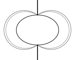
Figure 6: Shifting of the ergosphere – depicted here for an extremal Kerr black hole with $\epsilon=0.2$.

Perhaps the most important result from our study however is the discovery that the conical nature of the spacetime is not in the form of a simple deficit angle at infinity. All previous studies have assumed that the string will simply redefine the nature of the $\varphi$-angle, but we find this is not the case. Of course, once spotted, this seems entirely natural, due to frame dragging around the black hole, but we stress that this is a new physical phenomenon and will lead to distinct features of the Kerr+vortex black hole. For example, the ergosphere will be shifted (see figure 6) and orbits around the black hole will be affected. We have plotted in figure 7 the impact of the correction on the ISCO’s of the Kerr black hole. However, the minute value of the cosmic string tension will most likely render this effect outside the range of observational precision.

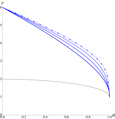
Figure 7: Shifting of ICSO’s as a function of $a$ (measured in units of $GM$) for $\epsilon=0,0.1,0.2,0.3$, represented by solid, dashed, dotted, and dot-dashed blue lines respectively. The black line indicates the location of the event horizon.

All in all, the vortex-Kerr system has proved to be surprisingly different and much more interesting that the standard Schwarzschild black hole hair.

- [1] P. T. Chrusciel, ’No hair’ theorems: Folklore, conjectures, results, Contemp. Math. 170, 23 (1994) [gr-qc/9402032].
- [2] J. D. Bekenstein, Black hole hair: 25 - years after, In Moscow 1996, 2nd International A.D. Sakharov Conference on physics 216-219 [gr-qc/9605059].
- [3] A. Achucarro, R. Gregory, and K. Kuijken, Abelian Higgs hair for black holes, Phys.Rev. D52 (1995) 5729–5742, [gr-qc/9505039].
- [4] R. Emparan, R. Gregory and C. Santos, Black holes on thick branes, Phys. Rev. D 63, 104022 (2001) [hep-th/0012100].
- [5] A. Vilenkin and E. P. S. Shellard, Cosmic Strings and other Topological Defects. Cambridge University Press, Cambridge, England, 1994.
- [6] H. B. Nielsen and P. Olesen, Vortex Line Models for Dual Strings, Nucl.Phys. B61 (1973) 45–61.
- [7] A. Vilenkin, Gravitational Field of Vacuum Domain Walls and Strings, Phys.Rev. D23 (1981) 852–857.
- [8] D. Garfinkle, General relativistic strings, Phys. Rev. D 32 (1985) 1323.
- [9] M. Aryal, L. Ford, and A. Vilenkin, Cosmic strings and black holes, Phys.Rev. D34 (1986) 2263.
- [10] R. Gregory, Gravitational stability of local strings, Phys.Rev.Lett. 59 (1987) 740.
- [11] J. Ipser and P. Sikivie, The Gravitationally Repulsive Domain Wall, Phys. Rev. D 30, 712 (1984).
- [12] G. W. Gibbons, Global structure of supergravity domain wall space-times, Nucl. Phys. B 394, 3 (1993).
- [13] R. Gregory and M. Hindmarsh, Smooth metrics for snapping strings, Phys.Rev. D52 (1995) 5598–5605, [gr-qc/9506054].
- [14] D. M. Eardley, G. T. Horowitz, D. A. Kastor and J. H. Traschen, Breaking cosmic strings without monopoles, Phys. Rev. Lett. 75, 3390 (1995) [gr-qc/9506041].
- [15] S. W. Hawking and S. F. Ross, Pair production of black holes on cosmic strings, Phys. Rev. Lett. 75, 3382 (1995) [gr-qc/9506020].
- [16] R. Emparan, Pair creation of black holes joined by cosmic strings, Phys. Rev. Lett. 75, 3386 (1995) [gr-qc/9506025].
- [17] A. Achucarro and R. Gregory, Selection rules for splitting strings, Phys. Rev. Lett. 79, 1972 (1997) [hep-th/9705001].
- [18] M. Dehghani, A. Ghezelbash, and R. B. Mann, Abelian Higgs hair for AdS - Schwarzschild black hole, Phys.Rev. D65 (2002) 044010, [hep-th/0107224].
- [19] A. Ghezelbash and R. Mann, Vortices in de Sitter space-times, Phys.Lett. B537 (2002) 329–339, [hep-th/0203003].
- [20] A. Chamblin, J. Ashbourn-Chamblin, R. Emparan, and A. Sornborger, Can extreme black holes have (long) Abelian Higgs hair?, Phys.Rev. D58 (1998) 124014, [gr-qc/9706004].
- [21] A. Chamblin, J. Ashbourn-Chamblin, R. Emparan, and A. Sornborger, Abelian Higgs hair for extreme black holes and selection rules for snapping strings, Phys.Rev.Lett. 80 (1998) 4378–4381, [gr-qc/9706032].
- [22] F. Bonjour and R. Gregory, Comment on ‘Abelian Higgs hair for extremal black holes and selection rules for snapping strings, Phys.Rev.Lett. 81 (1998) 5034, [hep-th/9809029].
- [23] F. Bonjour, R. Emparan, and R. Gregory, Vortices and extreme black holes: The Question of flux expulsion, Phys.Rev. D59 (1999) 084022, [gr-qc/9810061].
- [24] A. Ghezelbash and R. B. Mann, Abelian Higgs hair for rotating and charged black holes, Phys.Rev. D65 (2002) 124022, [hep-th/0110001].
- [25] A. N. Aliev and D. V. Galtsov, Gravitational Effects in the Field of a Central Body Threaded by a Cosmic String, Sov. Astron. Lett. 14, 48 (1988).
- [26] V. Cardoso, O. J. C. Dias, J. P. S. Lemos and S. Yoshida, The Black hole bomb and superradiant instabilities, Phys. Rev. D 70, 044039 (2004) [Erratum-ibid. D 70, 049903 (2004)] [hep-th/0404096].
- [27] V. Cardoso and O. J. C. Dias, Small Kerr-anti-de Sitter black holes are unstable, Phys. Rev. D 70, 084011 (2004) [hep-th/0405006].
- [28] A. Vilenkin, Cosmic strings and domain walls, Phys. Rep. 121 (1985) 263–315.
- [29] E. B. Bogomolnyi, The stability of classical solutions, Sov. J. Nucl. Phys. 24 (1976) 449.
- [30] R. Wald, Black hole in a uniform magnetic field, Phys.Rev. D10 (1974) 1680–1685.
- [31] D. V. Galtsov and E. Masar, Geodesics In Space-times Containing Cosmic Strings, Class. Quant. Grav. 6, 1313 (1989).
- [32] C. Charmousis, D. Langlois, D. A. Steer and R. Zegers, Rotating spacetimes with a cosmological constant, JHEP 0702, 064 (2007) [gr-qc/0610091].
- [33] G. W. Gibbons, A. H. Mujtaba and C. N. Pope, Ergoregions in Magnetised Black Hole Spacetimes, [arXiv:1301.3927 [gr-qc]].