Focal Plane Wavefront Sensing using Residual Adaptive Optics Speckles

Abstract

Optical imperfections, misalignments, aberrations, and even dust can significantly limit sensitivity in high-contrast imaging systems such as coronagraphs. An upstream deformable mirror (DM) in the pupil can be used to correct or compensate for these flaws, either to enhance Strehl ratio or suppress residual coronagraphic halo. Measurement of the phase and amplitude of the starlight halo at the science camera is essential for determining the DM shape that compensates for any non-common-path (NCP) wavefront errors. Using DM displacement ripples to create a series of probe and anti-halo speckles in the focal plane has been proposed for space-based coronagraphs and successfully demonstrated in the lab. We present the theory and first on-sky demonstration of a technique to measure the complex halo using the rapidly-changing residual atmospheric speckles at the 6.5 m MMT telescope using the Clio mid-IR camera. The AO system’s wavefront sensor (WFS) measurements are used to estimate the residual wavefront, allowing us to approximately compute the rapidly-evolving phase and amplitude of speckle halo. When combined with relatively-short, synchronized science camera images, the complex speckle estimates can be used to interferometrically analyze the images, leading to an estimate of the static diffraction halo with NCP effects included. In an operational system, this information could be collected continuously and used to iteratively correct quasi-static NCP errors or suppress imperfect coronagraphic halos.

1. Introduction.

Extrasolar planets (ESPs) are expected to be $10^{6}$–$10^{9}$ times fainter than their host stars in the thermal infrared. Solar system analogues will have planetary orbital distributions within one arcsecond of their host star (Nielsen, 2011), where they are masked by diffracted and scattered starlight. Without a coronagraph, most ESPs will appear to be several decades fainter than the telescope diffraction pattern, characterized by its point spread function (PSF). A coronagraph suppresses the diffraction structures in the PSF halo, but wavefront aberrations, alignment errors, and dust or other transmission flaws within the telescope scatter starlight into the suppressed region, overwhelming the faint science signal from the ESP. Ground-based telescopes rely on adaptive optics (AO) to correct the atmospheric wavefront distortions, but even a high degree of correction leaves random, rapidly-changing, residual speckles that are several decades brighter than the ESPs. Ideally, long exposures should average out the speckle noise as $1/\sqrt{t}$ to a level where the planet becomes detectable against a smooth background. Unfortunately, any unsuppressed halo is coherently modulated by the AO speckles, increasing the speckle noise (Bloemhof, 2004; Aime & Soummer, 2004), and AO processing lag can cause the residual speckles to be both brighter and persist longer than they otherwise might (Fried, 1990; Angel, 2003). The most serious features in the scattered starlight are quasi-static speckles (QSS) caused by non-common-path (NCP) aberrations (Racine et al., 1999; Hinkley et al., 2007), which are not known a priori, change on timescales from minutes to hours, and average slowly—if at all (Macintosh et al., 2005; Sivaramakrishnan & Oppenheimer, 2006). These halo features determine the practical detection limit for ESPs.

A number of techniques have been developed to address QSS and the effect of slowly-changing PSFs over time. These techniques include Angular Differential Imaging (ADI) (Marois et al., 2006; Schneider & Silverstone, 2003), Simultaneous Differential Imaging (SDI) (Biller & Close, 2007; Racine et al., 1999; Marois et al., 2000), and Local Optimization of Combined Images (LOCI) (Lafrenière et al., 2007), all with various degrees of success. These techniques all post-process the science camera data after observation time, and therefore can only achieve incoherent gains. AO systems include a deformable mirror (DM) that can dynamically modify the incoming wavefront, allowing wavefront correction to be introduced pre-detection, with the potential for coherent improvements in the signal gain. In an AO system, after encountering the DM, part of the starlight is diverted into a wavefront sensor (WFS), where the wavefront shape is measured and processed by a computer, sending updated compensating shape commands to the DM. The resulting flattened starlight wavefront may optionally be used to feed a coronagraph or imaged directly onto a science camera. In either case, NCP aberrations that occur downstream from the AO system are only evident in the final science images. This can manifest as distorted and fainter images or coronagraphically-suppressed halos that are spoiled by scattered starlight. But if instead of correcting the wavefront from the vantage of the WFS, we can try to improve the science image (Malbet et al., 1995) by applying bias offsets to the DM, we can obtain coherent gains that are significantly better than those achieved post-detection. Suppressing the halo also suppresses the interference or “pinned” speckle noise (Bloemhof, 2004), with a corresponding improvement in sensitivity. The problem is determining the correct biases to apply.

Uniquely improving the PSF (or the Strehl ratio) or suppressing undesired halo in a coronagraph using information from the science camera, requires more than just intensity measurements: it requires phase as well. A full complex halo measurement can be inverse Fourier-transformed to estimate the NCP optical flaws, interpreted under the paradigm of Fourier optics. The Strehl ratio can be improved by biasing the DM with the opposite of the computed pupil wavefront. Coronagraphic halo suppression can be improved by measuring the residual halo’s complex amplitude and creating a set of “anti-speckles” by adding ripples to the DM to suppress them (Codona & Angel, 2004). It is possible to build a modified Lyot coronagraph that uses the blocked starlight to form a reference beam (Angel, 2003; Codona & Angel, 2004) in a focal plane interferometer. However, measuring the halo with the science camera requires that the reference beam be included, spoiling the image unless exposures are multiplexed between interferometer and science. The two modes will have have similar exposure times if we are to measure faint static speckles that are of the same level of brightness as a planet, and the corresponding loss of science exposure time leads to a loss in sensitivity.

Another approach is to use the upstream DM to create weak probe speckles in the focal plane with controllable phase. The speckles coherently add to the underlying halo and interfere, modulating the intensity which is then recorded by the science camera (Bordé & Traub, 2006; Give’on et al., 2007). By using three or more probe speckle phases it is possible to measure the complex amplitude of the static halo under the probe speckle. This method works very well and is the basis for the extraordinary laboratory halo suppression results at the JPL High-Contrast Imaging Testbed (HCIT) (Trauger & Traub, 2007), designed to simulate a very stable space-based environment. Implementing this on the ground has to also contend with the presence of residual AO speckles, as well as a much less stable environment where at least the quasi-static speckles are changing on the timescale of a few minutes (Hinkley et al., 2007; Martinez et al., 2012), forcing the the probe speckles to be brighter in order to speed the measurements. Regardless of how the complex halo measurements are made, the same anti-halo servo algorithms can be applied or, if the the entire complex halo is available, Strehl ratio improvements can be achieved at the science camera. The downside of using a speckle probing method is the same as the coronagraphic focal plane interferometer: it puts probe light into the science image, forcing science and wavefront sensing to be multiplexed, reducing sensitivity.

In this paper we present and demonstrate a new technique for measuring the complex halo in the focal plane using only the residual AO speckles. Since the speckles are already present in the field of view, no extra light is introduced during the measurement, hence there is no need to reduce science exposure time. Since the AO speckles vary rapidly, measurements of both quasi-static speckles and other halo structure can be obtained fast enough to implement focal plane servos with update rates of several times per minute. Our method does not attempt to control the residual AO speckles, but only uses the WFS telemetry to monitor and characterize them as they change. The method requires no new hardware and should be implementable on virtually any AO system. The only requirements are that the science camera be capable of sufficiently short exposures ($\lesssim$ 30 ms) to adequately “freeze” the speckles, and that the camera and WFS data be accurately synchronized. In an earlier paper (Codona et al., 2008), we proposed an algorithm called “Phase Sorting Interferometry” (PSI), which binned and sorted the pixels based on the computed speckle phase. That result gave the static halo’s phase, which is the information needed to properly place a DM ripple in an anti-halo servo. In the present paper we greatly simplify the analysis into a set of statistical formulae that can easily be computed in real time. If the halo is estimated over only a limited search area, as it would be with a coronagraph, the results can be used to suppress the residual halo. If the halo is estimated more globally, including the PSF core, the result can also be used to estimate and correct the NCP aberrations, improving Strehl ratio and PSF quality at the science camera.

Our technique is most closely related to the random phase diversity techniques employed by Lee et al. (1997) and more recently by Frazin (2013). In those papers the focal plane intensity is written as a nonlinear functional of the unknown NCP aberrations, as well as the known residual AO wavefront error. The NCP error is then estimated from a synchronized set of focal plane images, simultaneous WFS measurements, and a nonlinear algorithm. In contrast, our approach is primarily to create the functional equivalent of a focal plane interferometer that measures the mean halo field. Once known, the linear relationship between the focal plane and pupil plane fields can be used to estimate the mean pupil field. If desired, the aberrated wavefront may then be estimated by computing the complex argument of the mean pupil field. Our approach never requires a nonlinear algorithm to estimate the pupil wavefront, the phase nonlinearity being completely contained within the calculation of the pupil field argument.

In Section 2 we present the theory of interferometry using a known-but-random probe field. In section 3 we simulate an AO system with NCP aberrations and apply the theory to the simulated data set. We demonstrate the robustness of the estimated complex halo and derived NCP aberrations by adding a wide range of noise in the science images. In Section 4 we use Shack-Hartmann WFS data from the MMTO 6.5 m telescope and short-exposure images from the Clio mid-infrared camera to estimate the complex halo. By Fourier transform, we estimate the complex pupil field including the effect of subsequent NCP aberrations. Using a 7th magnitude test star, reasonably consistent NCP aberration estimates were available in a few seconds. More stable estimates would required longer integrations, but an update to a possible NCP-correcting servo would be possible every 30 seconds or more.

2. Theory

We begin by considering a set of short-exposure images of a star, acquired while the telescope’s AO system is delivering diffraction-limited images with a clearly visible PSF core. The images consist of a static halo (the diffraction pattern of the telescope) and a cloud of rapidly-changing speckles. The speckles are significantly fainter than they would be be without the AO system, but they are still present and contribute scattered starlight out to the radius of the seeing disk and beyond. The science camera is unable to directly measure the incident electrical field’s phase, only the intensity of the static halo as it is modulated and coherently interfered with by changing speckle cloud. To see the speckles and their interference clearly, the individual exposures must be short enough that the speckles do not change much in phase or amplitude. The residual speckles arise from several sources: wavefront correction errors from noise in the wavefront sensing, limitations or errors in the wavefront reconstruction, AO servo errors (e.g. loop gain), fitting errors due to the deformable mirror, and processing lag. Of these, lag error speckles are the most dynamic since they are related to the wind along the telescope’s line of sight. The speckle cloud typically appears as diffraction-limited noise, with individual speckles having widths of $\sim\lambda/D$. But the halo also contains speckles and possibly deformations and extended regions of scattered starlight with much longer timescales. These include the quasi-static speckles which confusion-limit sensitivity in high-contrast detection. For our discussion, we consider these more slowly-changing features to be a part of the “static” halo, and by measuring its complex amplitude we can provide an adaptive anti-halo servo algorithm with the information required to correct aberrations or suppress unwanted halo and maximize sensitivity.

Whatever the cause of the rapidly-changing uncorrected wavefront error, and certainly in the case of lag error, the WFS residuals are non-zero and can still be measured. While the continuing goal for high-end AO systems is to reduce the residual wavefront error to below the WFS noise floor, we are not there yet. It is true that some of the residual error cannot be seen by the WFS, but in the current generation of AO systems there is always statistically-significant measurable wavefront error while the AO system is in closed loop. We will assume that we are in that situation. Any unsensed but varying residual will appear to us as unexplained noise in the image data. Changes that are averaged over during the science exposures will appear as a loss of coherence. Classic errors such as waffle are not a problem with the MMT since the hexapolar actuator pattern is incommensurate with the WFS subapertures. It might be an issue when implementing this method on other AO systems however.

Even though the Taylor “frozen flow” hypothesis (i.e. the approximation that turbulent motion of the atmospheric irregularities may be ignored as they are carried past the telescope’s line-of-sight by the wind) may be nearly true for the incident uncorrected wavefront aberrations, the residual AO wavefront error does not behave the same way. Consider a typical low-altitude wind that carries atmospheric irregularities across the 6.5 m MMT aperture in about 0.5 s. High altitude winds are typically much faster and cross the aperture in about 100 – 200 ms. In either case the irregularities are not likely to significantly rearrange during the pupil crossing. Turbulence within the observatory dome or in the vicinity of the telescope optics are different and significant rearrangement is likely. The AO system estimates the wavefront error and approximately removes it after a processing delay. It does this using a wavefront error-suppressing servo with an adjustable gain factor. As a particular wavefront pattern crosses the pupil, the AO system iteratively measures the residuals and adds corrections to the DM. Even for rapidly-moving wavefront patterns, the AO system has many tens to hundreds of iterations to suppress it. As a result, the residual pattern is usually incrementally altered as it moves across the pupil, becoming progressively more uncorrelated with its earlier configuration as it moves. The effect of an incorrect servo gain is that any pattern will not be completely removed in the next iteration. This repeats even while the initial pattern is being carried across the pupil, leaving a residual wavefront pattern that exponentially decays in-place with a time constant that depends on how far the gain is from the “correct” value. Thus the residual wavefront error is typically dominated by two or possibly three parts: a set of changing wavefront patterns that appear and disappear with a time scale dependent on the servo gain, and one or two wind-driven patterns that decorrelate much faster than turbulent rearrangement would suggest. Meanwhile in the focal plane, the wind-driven lag error forms a wide plume of speckles that are brighter near the star. In addition, as the wavefront errors move across the pupil, the speckles’ complex phasors rotate at a speed which increases linearly with distance from the star projected along the direction of the wind (Angel, 2003). Eventually, the phase wrapping is so fast that the speckle phase changes significantly during a single science camera exposure, causing the speckle and the static halo to appear to lose coherence in that interference between them has less contrast. Superimposed on this systematic effect is a random evolution of the speckles that depends on how long it takes to replace the pupil-plane aberrations with a statistically unrelated set. This is usually a fraction of $D/\left\|\mathbf{v}_{wind}\right\|$. These effects, along with the general fading of the speckle halo with angular distance from the star creates a practical outer radius for using speckles as a halo measuring tool. Fortunately, the generally brighter and slower speckles nearer the star allow us to measure the aberrations that affect telescope or coronagraphic performance exactly where improvement is needed most.

In isolation, the phase of a speckle is unobservable with the science camera unless the speckle coherently interferes with the static halo. But the cloud of rapidly-changing residual AO speckles do constantly interfere with the halo, making an intricate pattern of intensity fluctuations that can be captured by the science camera. Using the WFS telemetry and an idealized model for the telescope that ignores NCP errors, we can compute the phase and amplitude of the speckles at the science camera. Comparing these calculated speckles with the intensity recorded by the camera allows us to use the speckles as interferometric probes, enabling estimation of the phase and amplitude of the static halo. This relies on a simple concept: when the speckles are in phase with the underlying halo, the intensity is greater, and when they are anti-phased the combined intensity is diminished. If we were to plot the observed halo brightness against the speckle phase (Fig. 1), the maximum in the light curve corresponds to the phase of the halo at that point. In addition to the phase, an estimate of the static halo’s amplitude can be found by comparing various statistics computed from the science images and the computed speckles.

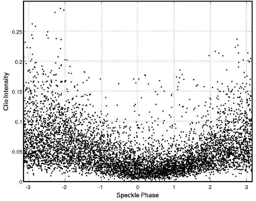
Figure 1.— Complex halo measurements using MMT data for a single pixel in the first Airy ring. The science camera intensity is plotted against the speckle phase computed from the WFS measurements. The speckles vary randomly in phase and amplitude while the underlying halo is presumed to be steady. When the speckle phase is the same as the halo, the intensity recorded by the science camera is increased. When the phase is $180^{\circ}$ off from the halo, the intensity is reduced. If the speckle amplitude were constant, the intensity would vary sinusoidally with speckle phase. The randomly-varying amplitude causes the sinusoid to become noisy, but the mean behavior is the same. Just judging by eye we can see that the underlying halo has a phase of about -2.5 rad in this pixel. Statistical analysis allows for much more precise estimation of the halo phase. Intensity scatter vs. intensity swing allows us to estimate the underlying halo amplitude. See Sec. 4 for details.

We begin by deriving the interferometry equations needed to use an ensemble of known random (in the sense of measured but uncontrolled) reference beams to estimate a static subject beam. We then apply the resulting equations to the problem of random speckles and a static halo. Since we do not have any a priori knowledge about the NCP aberrations, our calculations of the complex speckle field can only be approximate. However, the phase of the speckle peaks and their locations are able to be computed rather robustly and the effects of the unknown NCP errors will only enter as “speckles on the speckles” which will appear as a small amount of noise in our measurement.

2.1. Traditional Interferometry Theory

Since we have the ability to create speckles in the science camera’s focal plane by impressing a ripple on the DM, we could simply cycle through three or more ripple phases (i.e. by changing the ripple placement relative to the pupil) and determine which placement reinforces or suppresses the static halo under the resulting speckle (see Give’on et al., 2007; Kenworthy et al., 2006). The analysis is straightforward and equivalent to the common interferometry technique of using a phase-shifted reference beam to probe an unknown subject beam. In that generalized case the subject beam under test is mixed with a phase-shifted reference beam and a camera is used to capture the resulting interference pattern or “interferogram.” Using residual AO speckles is similar to using intentionally created speckles, except that they vary randomly in both phase and amplitude and are beyond our control. Even though the evolution is random, we can still measure the residual wavefront and determine the speckle amplitude and phase by calculation. The temporal evolution of the speckles is only important in that they might change during a single science camera exposure, smearing the parameters that we would like to use in interpreting the resulting image. Otherwise, the random speckles can be thought of as instantaneous samples drawn from an ensemble described by statistical moments. Interferometry with a random collection of reference beams (or speckles) looks different than the conventional analysis with carefully selected phases and a constant amplitude, but the principles are the same. Therefore, we will start by reviewing phase-shift interferometry, but use terminology that extends cleanly to our random speckle case. Both the traditional and generalized theory described below can be applied to measuring fields in any optical plane or physical context, but we will only consider its application in the focal plane in this paper. The traditional goal is to measure the phase of a constant subject beam $\SS$ by mixing it with a constant reference beam $\psi$ that is stepped through a set of known phase offsets. At each phase offset the camera is used to capture an intensity interferogram that is the magnitude-squared of the sum of the subject and phase-shifted reference beam fields. In our treatment we consider a single pixel of the camera and the fields are complex constants with phases $\phi_{s}=\arg\SS$ and $\phi_{r}=\arg\psi$ (where for $\psi=\left|\psi\right|\exp\left\{i\phi\right\}$, $\phi=\arg\psi\equiv\Im\ln\psi$). The reference beam is phase-shifted by an extra amount $\eta\in\{\eta_{n}\}$. To solve for the subject beam, we need at least three phase shifts in order to uniquely determine the phase. Even though everything here is constant or preset, we will use angle bracket notation $\left\langle\cdot\right\rangle$ to indicate averaging over an appropriate or indicated set. This will simplify the notational transition to randomly-varying reference beams easier. We require that the phase shifts are selected such that

$$\left\langle\exp\left\{i\eta_{n}\right\}\right\rangle\equiv\frac{1}{N}\sum_{n=1}^{N}e^{i\eta_{n}}=0.$$ (1)

If this condition is not met, the non-zero-mean reference beam will leave a residual that cannot be distinguished from being part of the subject beam. Our analysis will therefore produce the correct value biased by the mean of the reference beam. We also require that

$$\left\langle\exp\left\{2i\eta_{n}\right\}\right\rangle=0$$ (2)

so that we may easily process the interferograms. The interferograms record the intensity of the interfering fields at each of the applied phase shifts, giving

$$I_{n} = \left|\SS+\psi e^{i\eta_{n}}\right|^{2}$$ (3)

$$= \left|\Psi\right|^{2}+\left|\psi\right|^{2}+\SS\psi^{*}e^{-i\eta_{n}}+\SS^{*}\psi e^{i\eta_{n}}$$ (4)

$$= \left|\Psi\right|^{2}+\left|\psi\right|^{2}+2\left|\psi\right|\left|\Psi\right|\cos(\phi_{s}-\phi_{r}-\eta_{n}).$$ (5)

The expanded real form in Eq. 5 is the most familiar, but we prefer Eq. 4 because the complex algebra is simpler. We proceed by assigning each interferogram to the shifted complex phase of the reference beam and averaging over the phase shifts

$$\left\langle I_{n}e^{i\eta_{n}}\right\rangle=\left(\left|\Psi\right|^{2}+\left|\psi\right|^{2}\right)\left\langle e^{i\eta_{n}}\right\rangle+\SS\psi^{*}+\SS^{*}\psi\left\langle e^{2i\eta_{n}}\right\rangle.$$ (6)

Making use of our constraints Eqs. 1 and 2, we find that the mean intensity term averages to zero, and one of the two varying interference terms is “stabilized” while the other averages to zero by construction. The single surviving term is the product of the subject and conjugated reference beam

$$\left\langle I_{n}e^{i\eta_{n}}\right\rangle=\SS\psi^{*}.$$ (7)

Taking the imaginary part of the log of Eq. 7, we find the subject beam phase to be

$$\phi_{s}=\arg\left\langle I_{n}e^{i\eta_{n}}\right\rangle+\phi_{r}.$$ (8)

In many interferometric applications, the only desired quantity is the subject beam phase, in which case we are done. In cases where the subject beam amplitude is also desired, it can be found by simply blocking the reference beam and measuring the non-interfering intensity. But since we cannot “turn off” the speckles, along with the fact that the speckle cloud’s shape and amplitude fluctuates with the wind and other external influences and may not be accurately known, we will now find the subject beam amplitude assuming the reference beam amplitude is unknown. From Eq. 4 we find the average intensity as

$$\left\langle I\right\rangle=\left|\Psi\right|^{2}+\left|\psi\right|^{2}.$$ (9)

The magnitude-squared of Eq. 7 gives us the product of beam intensities

$$\left|\left\langle I_{n}e^{i\eta_{n}}\right\rangle\right|^{2}=\left|\Psi\right|^{2}\left|\psi\right|^{2}.$$ (10)

Note that $\SS$ and $\psi$ are interchangeable in both of these equations. Using Eqs. 10 and substituting in Eq. 9 and solving for the subject beam intensity,

$$\left|\Psi\right|^{2}=\frac{\left\langle I_{n}\right\rangle}{2}\pm\frac{1}{2}\sqrt{\left\langle I_{n}\right\rangle^{2}-4\left|\left\langle I_{n}e^{i\eta_{n}}\right\rangle\right|^{2}},$$ (11)

we find two solutions. This is due to the subject-reference ambiguity built into the statement of the problem. Which beam was physically phase shifted in our measurements is lost when looking at the intensity, and we are left with two solutions: one being the subject beam intensity and the other the reference beam intensity.

2.2. Interferometry with a known random reference beam

The analysis in Sec. 2.1 is very rigid in its reference beam variation, the main purpose being to simplify the mathematics. But we can also use a randomly-changing reference beam to analyze a static subject field $\SS$ in each pixel of a set of images in a manner very similar to Sec. 2.1. Being “random” in this context means not being controlled or predictable. “Random” does not imply that the reference beam is unknown, since we will always assume that at least its phase is known. If we know both the reference beam’s phase and amplitude corresponding to a series of images, the problem is very similar to the phase-shifted reference beam case above. Unlike that analysis however, which was unable to tell the difference between subject and reference beam phase and amplitudes, the varying reference beam allows us to unambiguously solve for both the subject beam since it is constant while the reference beam changes. If all we know about the reference beam is its phase, we can still estimate the subject beam’s phase by using the known reference beam phase to stabilize one of the fluctuating terms in Eq. 4. Even though the amplitude is changing, this allows a reliable statistical estimate of what reference phase maximizes the intensity (Fig. 1). When the intensity is maximized, the subject and reference phases are the same. If we also know the reference beam amplitudes, or even if we just know the rms speckle amplitude, we can determine the subject beam amplitude. Since our reference beam is determined by calculation from the WFS measurements and does not depend on, for example, the flux of the star (Sec. 4.4), we also have a scale factor between reference and subject beams that needs to be determined from the data’s statistics.

In Sec. 2.1, we typically had 3 or 4 images with known phase offsets. For the random reference problem, we imagine having a synchronized pair of relatively large data sets: one of complex reference beam fields and the other of the corresponding intensities. We treat each synchronized collection of images and fields as a set with statistics determined from the available data. We make no assumptions about underlying probability distributions.

The total field is the sum of the subject and reference fields, with the reference beam changing without the need for a separate phase offset

$$\Psi_{total}=\Psi+\psi.$$ (12)

The subject field $\Psi$ is assumed to be constant over the data set, while the reference beam $\psi$ changes in some uncontrolled yet measured or otherwise known way. The first assumption is that the reference beam field has a zero mean, functionally corresponding to the reference phase shift requirement in Eq. 1, but allowing for varying amplitudes,

$$\left\langle\psi\right\rangle=0.$$ (13)

If we were analyzing an ensemble of data, this would have some more absolute meaning. But since it is just the mean over the available data, perhaps spanning just a few seconds, the mean will have some random residual. This residual will appear to be part of the static subject beam, affecting the derived subject beam as estimation error. If the reference beam mean is non-zero, we can subtract it from the complex reference values and proceed using Eq. 13

$$\Psi_{total}=\left(\Psi+\left\langle\psi\right\rangle\right)+\left(\psi-\left\langle\psi\right\rangle\right).$$ (14)

The analysis will now yield the biased result $\left(\Psi+\left\langle\psi\right\rangle\right)$, from which the means may be subtracted at the end of the calculation. For simplicity, we will continue to write the reference field with the suppressed mean as $\psi$ which makes Eq. 13 true by construction. In addition to Eq. 13, we note that the mean square (not conjugated) of the field becomes negligible in large data sets,

$$\left\langle\psi^{2}\right\rangle\rightarrow 0.$$ (15)

This is the analog of Eq. 2 and cannot be independently forced like the mean. In our case where the speckles (our reference beam) are each the sum of many independent patches of approximately-flattened field across the pupil, the complex speckle field tends toward a Gaussian distribution by the central limit theorem (App. A). Note that for a zero-mean Gaussian random field, the scatter in estimates of $\left|\left\langle\psi^{2}\right\rangle\right|\propto 1/\sqrt{N}$ where $N$ is the number of statistically-independent speckles in each data set (App. B). The same is true of any moment $\left\langle\psi^{n}\left(\psi^{\star}\right)^{m}\right\rangle$ where $n\neq m$. We only require this general result for one more term, where the scatter in estimates of $\left\langle\psi\psi^{\star}\psi\right\rangle\rightarrow 0$ as $1/\sqrt{N}$ which is likely true so long as the speckle intensity and phase are uncorrelated (see App. B).

We start as before with a simple intensity model, leaving out any questions of partial coherence or intensity-dependent noise. We simply treat the static halo as a complex constant coherently interfering with the changing but known reference field. The resulting intensity is given by

$$I = \left|\SS+\psi\right|^{2}$$ (16)

$$I = \left|\Psi\right|^{2}+\left|\psi\right|^{2}+\SS\psi^{*}+\SS^{*}\psi.$$ (17)

Taking the average of Eq. 17 and invoking $\left\langle\psi\right\rangle=0$, we find the subject beam intensity is

$$\left|\Psi\right|^{2}=\langle I\rangle-\langle\left|\psi\right|^{2}\rangle\equiv\Phi_{I}-\Phi_{speckles}.$$ (18)

To facilitate our use of these results in later sections, we have also written the result in terms of physical measurables: $\Phi_{I}\equiv\langle I\rangle$ is the mean PSF recorded by the science camera and $\Phi_{speckles}\equiv\langle\psi\psi^{\star}\rangle$ is the average intensity of the halo of speckles if they were recorded on their own. Note that while the intensity expressed in Eq. 17 is real, each of the conjugated cross terms $\SS\psi^{*}$ and $\SS^{*}\psi$ rotate in opposite directions and individually have zero means. We can stabilize the first of the fluctuating terms in Eq. 17 by multiplying through by $\psi$, maintaining a stable phase while causing the other term to move twice as fast in phase. Upon averaging, the stabilized term survives and the others drop out giving

$$\left\langle\psi I\right\rangle=\langle\left|\psi\right|^{2}\rangle\SS\equiv\Phi_{speckles}\SS.$$ (19)

In writing this equation, we also made use of our assumption that $\langle\left|\psi\right|^{2}\psi\rangle\rightarrow 0$ even though it will not be precisely zero for a shorter data set, but will be in a larger data set. Since $\langle\left|\psi\right|^{2}\rangle\in\mathbb{R}$, we can immediately determine the phase of the subject beam as

$$\arg\Psi=\arg\left\langle\psi I\right\rangle,$$ (20)

which is the robust result we described in Codona et al. (2008). Since the reference beam intensity must be non-zero in order to make any measurement at all, we can simply write the subject field as

$$\Psi=\frac{\left\langle\psi I\right\rangle}{\langle\left|\psi\right|^{2}\rangle}\equiv\frac{\left\langle\psi I\right\rangle}{\Phi_{speckles}}.$$ (21)

2.3. Including an unknown scale factor

The subject beam field $\Psi$ is the static diffraction halo in the science camera focal plane. The reference beam field $\psi$ is the speckle field caused by the changing residual wavefront errors after the AO system has “corrected” the atmospherically-distorted incident field. The intensity $I$ measured by the science camera is proportional to the magnitude-squared of the sum of the static halo and speckle fields, but with the additional factors of incident flux and exposure time, etc. The speckle field is computed from WFS slopes with possible (modal) gain errors in the wavefront reconstruction, and generic assumptions about amplitude. Converting these fields to actual images require all of the aforementioned factors such as starlight flux. All of these influences can be included in an unknown scale factor $\mathit{g}$ that may also be a function of focal plane position. The relationships between $\Psi$, $\psi$, and $I$ depend on getting this scale factor right, so we will add it to the model and estimate it from the data. We introduce the scale factor into Eq. 16 with the modification

$$I=\left|\SS+g\psi\right|^{2}$$ (22)

where $g\in\mathbb{R}$ since we assume our phase estimates are accurate. Following our derivation as before, we find the mean intensity

$$\Phi_{I}=\left|\SS\right|^{2}+g^{2}\Phi_{speckles}$$ (23)

and the stabilized intensity

$$\left\langle\psi I\right\rangle=g\SS\Phi_{speckles}.$$ (24)

To determine the scale factor before we know $\Psi$, we adjust it until the intensity variance based on the calculated speckles matches that of the actual intensity images. Using Eq. 22 to compute $\sigma_{I}^{2}\equiv\langle\left(I-\left\langle I\right\rangle\right)^{2}\rangle$, we find

$$\sigma_{I}^{2}=2g^{2}\left|\SS\right|^{2}\Phi_{speckles}+g^{4}\sigma_{speckles}^{2}$$ (25)

where $\sigma_{speckles}^{2}=\langle(\left|\psi\right|^{2}-\langle\left|\psi\right|^{2}\rangle)^{2}\rangle$ is the speckle-only intensity variance without halo interference. Using the magnitude-squared of Eq. 24 to replace $g^{2}\left|\SS\right|^{2}$ with measured quantities in Eq. 25, we find

$$g=\left[\frac{\sigma_{I}^{2}}{\sigma_{speckles}^{2}}-\frac{2\left|\left\langle\psi I\right\rangle\right|^{2}}{\Phi_{speckles}\sigma_{speckles}^{2}}\right]^{1/4}.$$ (26)

Using this result in Eq. 24 allows us to write the halo as

$$\Psi=\frac{\left\langle\psi I\right\rangle}{g\Phi_{speckles}}.$$ (27)

This is the diffraction halo at the science camera, including any non-common-path aberrations. While it is obvious that the intensity imaged by the science camera must first have any background noise removed, it is important to note that the background noise variance should also be estimated and removed from $\sigma_{I}^{2}$ before using Eq. 27. We will also find that the region near the center of the halo (very low spatial frequencies) tends to be biased low due to physical reasons not included in our isolated pixel analysis. Since the result is still useful without increasing the complexity of the model to eliminate the bias, we will use these results as they stand.

2.4. Visibility

The traditional interference fringe “visibility” measures the intensity modulation caused by changing the reference beam phase normalized by the mean intensity (Born & Wolf, 1999, Sec. 7.5). It is usually written in terms of the max and min intensities as

$$V = \frac{I_{max}-I_{min}}{I_{max}+I_{min}}.$$ (28)

Since the standard deviation of the cosine is $\sqrt{2}$, we can use Eq. 5 to rewrite the conventional definition of visibility as

$$V=\frac{\sqrt{2}\sigma_{I}}{\left\langle I\right\rangle}.$$ (29)

In our random reference case, the appropriate portion of the intensity variance is the term in Eq. 25 that is caused by interference ($2g^{2}\left|\SS\right|^{2}\Phi_{speckles}$) rather than intrinsic variations in the reference beam intensity ($g^{4}\sigma_{speckles}^{2}$). This allows us to write

$$V=\frac{2g\left|\SS\right|\sqrt{\Phi_{speckles}}}{\left\langle I\right\rangle}.$$

Using Eq. 27 to replace $\left|\SS\right|$, and the notational association of $\left\langle I\right\rangle=\Phi_{I}$, the formula for the visibility becomes

$$V=\frac{2\left|\left\langle\psi I\right\rangle\right|}{\Phi_{I}\,\sqrt{\Phi_{speckles}}}.$$ (30)

3. Simulation

In this section we demonstrate our technique with a realistic simulation based on the MMTO 6.5 m telescope and AO system, with some arbitrary NCP errors added. Using the simulation results, we apply our random reference interferometric formulae to estimate the static complex halo and informally explore the effect of measurement noise. Finally, we Fourier transform the complex halo back into the pupil plane to estimate the NCP aberrations. We find that this method underestimates the very lowest spatial frequencies of the pupil field, requiring a simple correction to recover the proper static wavefront aberration. The results are adequate for building either an anti-halo servo for a coronagraph or improving the Strehl ratio at the science camera by compensating for NCP aberrations. Finally, we discuss the degradation of results caused by speckle halo evolution during the science camera exposures and how to estimate its effect from real data.

We used a simple lagged spatial filtering model to simulate the post-AO wavefront at the MMT. We first synthesized a $2048\times 2048$ grid with 4 cm spacing of Kolmogorov wavefront displacements scaled to give a Fried length $r_{0}$ of 15 cm in V band and an outer scale of 30 m. The effect of AO correction was simulated by applying a Gaussian smoothing to the wavefront and subtracting the result from the original wavefront. This approximates the effect of applying a mode-limited reconstructor to the DM. The width of the smoothing kernel was adjusted to make the rms residual wavefront fitting error (WFE) 250 nm. The effect of wind and processing lag was introduced by laterally shifting the smoothed correction by $\delta\mathit{\mathbf{x}}=v_{wind}\tau_{lag}$. For convenience, the lateral shift was selected to be one grid pixel of 4 cm. A total of 5 phase screens were synthesized and a set of residual wavefronts was selected from each by using a sub-grid of size $D=6.5$ m at $0.85D$ spacings giving a $14\times 14$ sample of slightly-overlapping wavefronts. Each scintillation-free pupil field instance was computed using $\exp\left\{2\pi i\delta\bm{z}/\lambda\right\}$ and multiplied by a 6.5 m pupil mask $\Pi(\mathit{\mathbf{x}})$ with a 10% central obstruction. The wavelength $\lambda$ was set to 3.8 $\mu$m (L’ band). In addition to the residual AO wavefront error, the camera images were presumed to include an additional non-common-path (NCP) wavefront error described by Zernike trefoil ($\delta\bm{z}=Z_{3}^{3}(2r/D,\theta)\,\lambda/16$) and an additional Gaussian indentation centered on $\mathit{\mathbf{x}}_{0}=(-1,2)$ (meters) with depth $\lambda/8$ (max mirror figure error of 237.5 nm) with a $1/e$ radius of 1 m (Fig. 2).

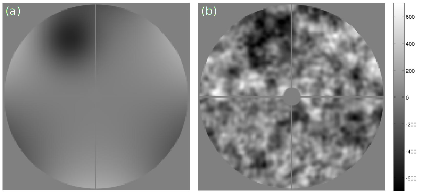
Figure 2.— (a) The simulated non-common-path error masked by the pupil. The modeled aberration includes trefoil and a Gaussian indentation. The peak-to-valley aberration is 725 nm. (b) The NCP error added to a realization of the residual AO residual WFE.

The PSFs were computed using 2-D FFTs padded to $2048\times 2048$ samples and taking the magnitude squared to find the intensity. The resulting images were converted to array counts assuming a mean total of 157,000 counts per exposure (typical of a magnitude 7.5 star at L’ band, bandwidth of 0.65 $\mu$m, MMT aperture, 50% QE, and a throughput of 67%). Gaussian noise was added to the images to simulate the variance caused by different amounts of thermal and sky background noise. The complex speckle halo was computed without the NCP aberrations, but with the same pupil mask. This takes the place of the WFS-based halo calculation in the actual observations. The intentional neglect of the NCP WFE in the halo calculation emulates the fact that we cannot see the downstream NCP errors when working from the WFS measurements. This “bootstrapping” technique of the algorithm should have minimal effect on the speckle phases so long as the Strehl ratio is high enough to have a clear peak above the speckles. (We tested the effect of this approximation by including the NCP errors in the speckle calculation, with an effect on the estimated wavefront error of 8 nm rms or about 0.013 radians rms.) The resulting complex halo has speckles with the ideal PSF’s sidelobes, as opposed to the actual speckle sidelobes which would show the trefoil, etc. The computed speckles are otherwise in the correct locations and have the correct phase relationship to the PSF core. After subtracting off the mean complex halo, the remaining speckles have mostly the correct complex values near their maximum amplitudes, where the effect of the simplified sidelobes can be ignored.

In a calculation of this sort, it is possible to know and control the piston component of the wavefront, resulting in absolute phase control or to have a global phase reference. This is not the case in reality however. The wavefront sensor only measures wavefront slopes and is therefore blind to constant phase offsets. The mean intensity distribution of the speckles, $\Phi_{speckles}$, has power and phase fluctuations all the way in to the center of the PSF. We multiply the complex halo by a unit-amplitude phasor to adjust the halo’s peak value to zero phase and reference the speckles to the current halo peak, allowing them to be compared. Ideally, we would want to reference the halo phase to the core of the static halo, but it is only practical to use the phase of the full computed complex halo. This will slightly bias the reference phase and introduce a fluctuating phase error to all points in the halo. This phase error is zero-mean and becomes less significant at higher Strehl ratios like those in our simulation. Our phase referencing procedure does not change either the speckles’ intensity or variance, which is why we correctly see speckle power all the way to the center of the PSF (Fig. 3). When we process real data, we also remove tip-tilt from the WFS measurements and the science images, which has the effect of further removing speckle power to the next order about the center of the PSFs. Again, this is not detrimental to the measurement of $\Psi$ away from the center, but it will bias the lowest spatial frequencies and become an issue when we attempt to estimate the pupil field from our focal plane results.

Once the complex halo was computed for all pupil wavefronts and all of the peaks were referenced to zero phase, the complex mean was computed and subtracted, leaving only the complex speckles $\psi$.

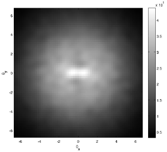
Figure 3.— The mean speckle halo intensity averaged over the simulated data set. The residual AO fitting error is isotropic, while the lag error driven by the wind ($\mathbf{v}_{wind}\tau_{lag}=4$ cm) is responsible for the horizontal plume of speckles near the center.

The mean speckle intensity is shown in Fig. 3. The figure clearly shows the broad fitting error cloud and a horizontal plume of speckles caused by lag error and the wind. There is no evidence of the main diffraction pattern in the speckle halo, since the appearance of aberrations in the simulation is independent of position relative to the pupil. To explore the robustness of the result, zero-mean Gaussian noise was added to the simulated CCD images to simulate observations of fainter target stars. The introduced noise sigmas are 0, 10, 100, and 1000 counts per pixel.

In order to use the random reference interferometry results, we need to compute various statistics from the simulated fields and images. The mean speckle field is zero by construction, leaving any actual non-zero means folded into the static halo as estimation error.

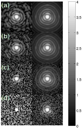
Figure 4.— Simulated science camera images: single frame (left) and data set averages (right). The images are constructed from the computed PSFs with photon noise and added background noise. The starlight is set to an average of 157,000 counts per exposure, with added background noise sigmas of (a) 0, (b) 10, (c) 100, and (d) 1000 counts per pixel. The PSF images are $15\lambda/D$ on each side with $0.25\lambda/D$ pixels. The simulation dataset included 980 images. The PSFs on the left are individual 20 ms images while those on the right are averaged over the 980 images in the entire data set (a total exposure time of 19.6 s).

The simulation generates two data cubes: a set of simulated science camera images with all aberrations included and actual counts per pixel, and a data cube of complex halos that, in reality, would have been computed from the WFS measurements and a simplified model of the telescope without the NCP aberrations. The mean of the complex halo data cube is an estimate of the static halo, but without the NCP distortions we wish to measure. This mean is subtracted from the complex halo cube leaving only the complex speckle field. While the computed speckle phases and relative amplitudes values are meaningful, the units are arbitrary and cannot be compared directly with the photon counts in the science camera image cube. So we include a scale factor $g$ (first introduced in Eq. 22) as a constant that depends on the flux and takes care of the units. The average of the science images gives $\Phi_{I}$ (Fig. 4), the average of the magnitude-squared speckle fields (the “speckle intensities”) gives $\Phi_{speckles}$ (Fig. 3), the variance of the science images is $\sigma_{I}^{2}$ (Fig. 5) and the variance of the speckle intensities is $\sigma_{speckles}^{2}$.

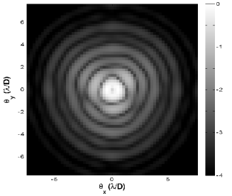
Figure 5.— The variance of the simulated science camera images $\sigma_{I}^{2}$ displayed on a 4-decade logarithmic scale. This figure only includes intensity variations caused by the changing speckles, with no background or photon noise. The science image variance includes the product of the speckle halo and the intensity of the static halo (Eq. 25). There is a reduction in the variance at the center as a consequence of the anti-Hermitian symmetry of speckles and is not included in our analysis model.

Since the two datasets are computed from the same grids, they are automatically commensurate and properly aligned. We multiply the science image and complex speckle field data cubes element-by-element and average over the 960 frames to compute $\left\langle\psi I\right\rangle$ from which we can derive the static complex halo $\Psi$ using Eq. 27 (Fig. 6).

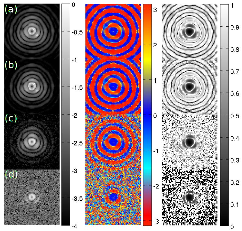
Figure 6.— The computed static halo and visibility at noise levels listed in Fig. 4. The leftmost column is the base-10 log of the static halo amplitude. The levels are normalized to a point in the first Airy ring. The center column is the computed phase of the static halo, and the rightmost column is the visibility (lighter is better). Note the missing intensity at the very center of the halo in the left column images. This is due to the anti-Hermitian symmetry of the speckles, an effect that is not included in our interferometry analysis.

Note that the static halo has a lower amplitude than it should at the very center of the function. This is caused by a subtle difference between our interferometric analysis and the symmetries of complex speckles. We assumed that an arbitrary random complex speckle could be added to the static halo anywhere during the interferometric analysis. This is true everywhere in the focal plane except at the center of the star image. The reason is that a small amplitude wavefront ripple in the pupil plane not only diffracts starlight from the PSF core into a speckle at the expected position, but creates another speckle on the opposite side of the star. Referenced to the starlight in the PSF core, the two speckles have different phases such that the real part of the field is antisymmetric, while the imaginary part is symmetric. This is called anti-Hermitian symmetry and is a well-known feature of faint speckles. Each speckle is able to take on an arbitrary complex value, subject to energy constraints, and the speckle on the other side of the star will follow according to its anti-Hermitian symmetry. This non-local correlation is not an issue in our analysis because the two correlated speckles are usually so far apart from each other that they have no mutual effect. However, a very low spatial frequency aberration, or even small residual tip-tilts, cause speckle pairs which appear close enough together that they can significantly interfere. When they do, the antisymmetric real part tends to cancel and the sum becomes only due to the symmetric imaginary part. Since we have constructed the phase reference to be the PSF core, ideally of the static halo center, the center of the static halo is real. Adding a small speckle near the core approaches purely imaginary and has the effect of a phase shift. This does not change the intensity of the PSF core, only the phase, therefore the intensity variance near the core should drop relative to where the speckle pairs don’t overlap (Fig. 5).

If we use our results in an anti-halo servo designed to suppress unwanted residual halo in a coronagraph, the low spatial frequency power deficit in Eq. 27 does not affect us. However, if we wish to estimate the wavefront in the pupil plane, as we might for increasing the Strehl ratio in the science images by correcting the NCP aberrations, or for computing a more accurate numerical PSF for post-detection processing of the science images, we would like to recover the low spatial frequencies as well as the higher ones. We can still do this by reconsidering how we compute $\left|\Psi\right|^{2}$. Instead of using Eq. 24 to compute $\Psi$, we compute the halo phase $\arg{\Psi}$, which is what we found in Eq. 20. We then estimate the static halo intensity from Eq. 23, which does not suffer from the anti-Hermitian speckle effect. To satisfy the requirement that $\left|\Psi\right|\in\mathbb{R}$ and $\left|\Psi\right|^{2}>0$, we use a $\max$ function, giving a better estimate of $\Psi$ as

$$\Psi=\sqrt{\max\left\{\Phi_{I}-g^{2}\Phi_{speckles},0\right\}}e^{i\arg\left\langle\psi I\right\rangle}.$$ (31)

We computed $\Psi$ using this equation and Fourier transformed back into the pupil plane to compare with the initial NCP aberrations. The results for a set of noise levels is shown in Fig. 7.

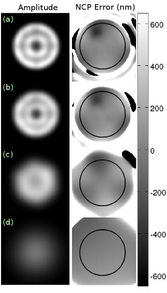
Figure 7.— Fourier transforming the static halo $\Psi$ computed from Eq. 31 gives an estimate of the static pupil field $\Upsilon$ for the same noise levels listed in Fig. 4. The left column is the amplitude of the estimated pupil field and the right column shows the pupil phase scaled to wavefront displacement in nm. As the noise level increases, high angles are lost first, leaving a progressively smoothed pupil wavefront estimate.

For each noise level, the pupil field amplitude is shown on the left and the phase converted back to nanometers of wavefront displacement is shown on the right, which should be compared with the introduced NCP aberrations. The spatial resolution is limited because the SNR drops off with increasing radius. As the noise level is increased, the estimated pupil field and wavefront becomes progressively smoother. The simulation is somewhat unrealistic in that the speckles were not derived from a Nyquist-limited WFS measurements and the wavefront itself has properties that are statistically “cleaner” than real data with residual wavefront errors that are not tied to the pupil or actuator locations. Nevertheless, the results validate the technique and show us what to expect with real data.

3.1. Effects of optical bandwidth and exposure time

In the preceding discussions, we assumed that the evolving halo field was monochromatic and instantaneously sampled in time, with no blurring or phase averaging due to speckle evolution during the exposure. However, these effects can be important in practice. The incident wavefront at a single point in the pupil experiences an rms phase change of 1 radian after a time $\tau_{0}$ defined by the phase structure function $D_{\phi}(\mathbf{v}_{wind}\tau_{0})=1$ , where $\mathbf{v}_{wind}$ is the characteristic wind velocity projected onto the pupil plane. This time scale determines how fast WFS exposures must be made as well as actuator and AO servo bandwidths. However, the speckles do not depend only on the field at a point, but the field across the entire pupil. Moving the pattern by a small distance, or even possibly by $r_{0}$, leaves most of the uncorrected incident wavefront unchanged, simply translated. This causes speckles to remain in the same place, but with a phase shift depending on the location of the given speckle in the focal plane relative to the wind. AO residual speckles are more complicated because they are the result of the initial aberrations and the spatial and temporal limitations of the AO system.

For atmospheres with visible $r_{0}$ values of $\sim 15$ cm and winds of $\sim 20$ m/s, $\tau_{0}\gtrsim 2$ ms. An AO wavefront sensor typically has readout speeds of 500 – 2000 frames/s, allowing the wavefront to be estimated at that frame rate. Limited photon flux degrades the wavefront estimate accuracy with increasing frame rate, as does decreasing star brightness or increasing background noise (Sandler et al., 1994). The MMT AO system is currently at the low end of the frame rate range, but still fast enough to capture the low spatial frequency wavefront evolution without significant averaging. Science cameras are usually used with much slower frame rates, although capabilities of 30 to 50 fps are not uncommon. Broader optical filter bandwidths pass more light, enabling us to make better use of higher frame rates. However, the broader filter bands also increase chromatic effects that can lead to confusion in the analysis.

Our MMT L-Band images have optical bandwidths of about 20% (0.7 $\mu$m bandwidth centered on 3.7 $\mu$m). This introduces chromatic radial smearing where both diffraction halo and speckle features appear at points proportionally farther from the star with increasing wavelength. A practical operational constraint is to not allow speckles and other halo features to radially blur into each other, beyond which they may become confusion-limited. The limits implied by this constraint can be estimated by noting that the typical monochromatic speckle size and separation are both $\sim\lambda_{0}/D$ ($\lambda_{0}$ is a characteristic wavelength in the detected band), regardless of their location relative to the star. At a radius $\theta$, the radial smearing is $\left(\delta\lambda/\lambda_{0}\right)\theta$. The non-overlap constraint gives us the condition

$$\theta<\left(\frac{\lambda_{0}}{\delta\lambda}\right)\frac{\lambda_{0}}{D}.$$ (32)

The MMT Shack-Hartmann WFS uses a $12\times 12$ sub-aperture array centered on the pupil, which means the maximum measurable unaliased spatial frequency is 6 cycles$/D$, beyond which we cannot compute the speckles. This corresponds to a fractional bandwidth of about 17%, which is reasonably well matched to the L band filter. Well inside the radial blurring limit, we are progressively more free to ignore the effects of bandwidth and simply use monochromatic Fourier optics (Goodman, 1995) at the characteristic wavelength $\lambda_{0}$.

Depending on the brightness of the star compared to the background noise and the shape of the speckle halo, the SNR of our measurement varies widely across the focal plane. A long science camera exposure will smooth the intensity fluctuations caused by the speckles beating against the static halo, reducing their contrast and making them harder to detect against the background noise and fluctuations. The WFS data, converted to complex speckles, also has to be integrated to the science camera’s frame rate in order to compare the complex speckles with the images. Our metric for signal is the “visibility” (Eq. 30), but that alone does not express the fluctuating signal relative to the background noise. The visibility is the phase-dependent intensity variation relative to the mean intensity. The proper metric for comparing the intensity variations, from which we derive all other information, and the background noise is

$$\mbox{SNR}=\frac{V\Phi_{I}}{\Phi_{noise}}=\frac{2\left|\left\langle\psi I\right\rangle\right|}{\Phi_{noise}\,\sqrt{\Phi_{speckles}}}.$$ (33)

The average intensities, $\Phi_{noise}$ and $\Phi_{speckles}$, are unaffected by the exposure time since they are sums of positive contributions. The impact of exposure comes only from the $\left|\left\langle\psi I\right\rangle\right|$ factor, which we can analyze. Treating $I(t)$ and $\psi(t)$ to be instantaneous measurements, we write the effect of longer camera exposures as an integral average of duration $T$ centered on $t=0$, and use an ensemble average to estimate the effect on $\left|\left\langle\psi I\right\rangle\right|$. In Eq. 33 we replace $I$ with an integrated $I$ to represent the time exposure

$$I(t)\rightarrow\frac{1}{T}\int_{-T/2}^{T/2}I(t+t^{\prime})\mathrm{d}t^{\prime},$$

and

$$\psi(t)\rightarrow\frac{1}{T}\int_{-T/2}^{T/2}\psi(t+t^{\prime})\mathrm{d}t^{\prime}.$$

Multiplying the down-sampled measurements and ensemble averaging, the stabilized intensity becomes

$$\left\langle\psi(t)I(t)\right\rangle\rightarrow\frac{1}{T^{2}}\iint_{-T/2}^{T/2}\left\langle\psi(t+t_{1})I(t+t_{2})\right\rangle\mathrm{d}t_{1}\mathrm{d}t_{2}.$$

Referring back to our simple model for the intensity, Eq. 22, we expand and multiply through by the field, performing the ensemble average on each term. Based on our assumption that the speckle field is ultimately a zero-mean Gaussian random process, the only term that survives averaging is $I(t)=g\Psi\psi^{*}(t)$. Thus

$$\left\langle\psi(t)I(t)\right\rangle\rightarrow\frac{g\Psi}{T^{2}}\iint_{-T/2}^{T/2}\Gamma(t_{2}-t_{1})\mathrm{d}t_{1}\mathrm{d}t_{2},$$ (34)

where $\Gamma(\tau)$ is the complex speckle field’s mutual coherence function (MCF)

$$\Gamma(t_{1},t_{2})=\left\langle\psi(t_{1})\psi^{\star}(t_{2})\right\rangle.$$ (35)

The MCF becomes time-invariant, depending only on the time difference, $\Gamma(t_{2}-t_{1})$ with the symmetry $\Gamma(\tau)=\Gamma^{*}(-\tau)$, so long as parameters such as wind, $r_{0}$, and AO performance remain constant. We can normalize the performance by the assuming that the camera exposures match the WFS, which gives the reference value of $\left\langle\psi I\right\rangle$ as

$$\left\langle\psi I\right\rangle\rightarrow g\Psi\Gamma(0)\equiv g\Psi\Phi_{speckles}.$$ (36)

We divide Eq. 34 by Eq. 36 to estimate the effect of exposure time on SNR. Changing time integration variables to sums and differences and using the MCF symmetry allows us to write the effect of exposure on SNR as

$$\mbox{SNR $\propto$}\frac{1}{T}\int_{0}^{T}\left(1-\frac{\tau}{T}\right)\Re\left\{\frac{\Gamma(\tau)}{\Gamma(0)}\right\}\mathrm{d}\tau.$$ (37)

We will use this result with the actual MMT data in Sec. 4.4.

The residual speckle halo $\Phi_{speckles}(\bm{\theta})\equiv\Gamma(t_{1},t_{1};\bm{\theta})$ consists of a broad fitting error halo along with lag error speckle plumes in the apparent projected direction of the wind. If there are multiple wind streams along the line of sight, they will each contribute their own speckle plume. Both fitting and lag error phase patterns are carried across the pupil by their respective winds, with characteristic effects expressed in the resulting speckles. For simplicity, we will consider only one dominant wind stream with velocity projected onto the pupil plane of $\mathbf{v}_{wind}$. Fitting error has minimal power in spatial scales larger than $\ell_{AO}\sim D/\sqrt{N_{modes}}$ and the corresponding halo is therefore dark within $\lambda/\ell_{AO}$, or at least relatively constant, depending on details of the AO system. Processing lag error contributes a residual wavefront that is proportional to the gradient of the uncorrected wavefront dotted into the wind shift after the lag (i.e. $\tau_{lag}\mathbf{v}_{wind}\cdot\nabla\phi_{0}$) since the wavefront correction servo makes the same error in every iteration. This leads to a plume of speckles in the direction of the wind that becomes brighter as we look closer to the star. Depending on the details of the AO system, the fitting error changes completely by the time the wind has carried the wavefront by the AO correction scale $\ell_{AO}$. Therefore, the fitting error speckles decorrelate after a timescale of $\ell_{AO}/\left\|\mathbf{v}_{wind}\right\|\lesssim\tau_{fitting}\lesssim D/\left\|\mathbf{v}_{wind}\right\|$ (a fresh breeze of 20 m/s at the MMT would give timescales of 43 ms$\lesssim\tau_{fitting}\lesssim$325 ms). Lag error speckles are still affected by larger spatial scales and can last much longer (App. A). These are certainly completely decorrelated by the time the wind has carried the turbulent pattern by the outer scale, $\tau_{wind}\lessapprox L_{outer}/\left\|\mathbf{v}_{wind}\right\|$ (possible on the order of a second or more at the MMT). The outer scale in all layers of the astronomical AO problem are often considered to be less than 30 m, but may be longer in special cases. The decorrelation timescales described here vary across the speckle halo around the star, and only real data can tell the actual behavior. But we can say a few things that ought to be robust statements. The fitting error speckles should decorrelate fairly rapidly, while lag error speckles should last significantly longer.

The same is not true of the translation effect, which is systematic and highly dependent on position. Translation of the residual wavefront by an amount $\delta\mathit{\mathbf{x}}$ causes any speckles at angular position $\bm{\theta}=\bm{\kappa}/k$, $k=2\pi/\lambda$, to undergo a phase shift of $\delta\phi=-k\bm{\theta}\cdot\delta\mathit{\mathbf{x}}$. (This ignores the overall change in coherence due to slightly different areas of the wavefront being visible through the pupil at different times, which is contained in the previously discussed portions.) Therefore, a wind will cause a linear phase shift $\delta\phi=k\bm{\theta}\cdot\mathbf{v}_{wind}\delta t$. This affects all of the speckles together systematically, and shows up in the MCF as

$$\Gamma(\tau)=\Gamma_{0}(\tau)e^{2ik\tau\bm{\theta}\cdot\mathbf{v}_{wind}},$$ (38)

where $\tau=t_{2}-t_{1}$.

We can now estimate the effect of science camera exposure time. We will consider only a single wind stream of ~10 m/s, noting that for a moderate frame rate of $\sim 30$ fps, a jet stream contribution with a speed of ~60 m/s will be highly averaged over virtually all of the focal plane, appearing as incoherent noise. For fitting error, the slow change in the MCF due to different configurations being present within the pupil has a timescale of ~650 ms but likely much shorter due to the AO iterations and other effects. Lag error speckles within the control radius but outside of the PSF core arise from spatial scales smaller than the pupil diameter $D$ and are most likely uncorrelated much beyond the pupil. Therefore they too have a maximum lifetime of hundreds of milliseconds, which is common. The systematic phase rotation caused by the wind increases most rapidly in the direction of the speckle plume and is not seriously detrimental until the phase wrapping from the time center of the exposure to the endpoints is $\pi/2$, beyond which negative contributions are included. This means that the phase rotation timescale, providing us with a conservative exposure time limit, is when $\pi>k\left|\bm{\theta}\cdot\mathbf{v}_{wind}\right|\mathsf{t}_{sci}$ or

$$\mathsf{t}_{sci}<\frac{D}{2\left|\frac{\bm{\theta}}{\lambda/D}\cdot\mathbf{v}_{wind}\right|}.$$ (39)

Using the WFS Nyquist radius for the MMT $12\times 12$ WFS along either axis, $\left\|\bm{\theta}\right\|=6\lambda/D$, and a wind of 10 m/s, we find that our exposure limit is about 54 ms. Assuming continuous exposures, that corresponds to about 18.5 fps. Referring back to the effect of decorrelation on the SNR, Eq. 37, we can see that our limit only drops the SNR by 64% at the limiting radius. Using a higher frame rate camera is therefore not extremely important for sensitivity, but would be for an increased measurement radius or for higher wind speeds.

4. Observations and Analysis

To measure the complex halo at the science camera, we require three capabilities: (1) acquire short exposures with the science camera, (2) AO wavefront sensor data, and (3) provide a mechanism for synchronizing the resulting data sets together. Our mid-IR camera is capable of reading out small regions of the sensor at frame rates in excess of 30 Hz, and our high-speed AO WFS and subsequent processing software has an engineering diagnostic mode capable of saving the full system telemetry, including raw WFS pixels and computed slopes. Tight synchronization between the science camera and the AO system is not provided by the MMT and is added using system handshaking and logging modifications. We describe our solutions to these generic problems here, as well as other difficulties to do with the engineering state of the MMT at the time of our observations.

4.1. Facilities

4.1.1 The MMT AO System

The MMT Adaptive Optics system (Wildi et al., 2002) is the world’s first telescope to use a deformable secondary mirror to provide wavefront correction. This approach minimizes the number of warm optical surfaces between the sky and the science camera, greatly reducing the thermal emissivity of the telescope, and makes the 6.5 m MMT aperture competitive with larger telescopes for thermal infrared observations (Lloyd-Hart et al., 2000). The 640 mm diameter deformable secondary consists of a thin shell mirror 2 mm thick, supported above a Zerodur reference body by a fixed central hub, and deformed by 336 actuators in a modified hexapolar pattern (Fig. 8).

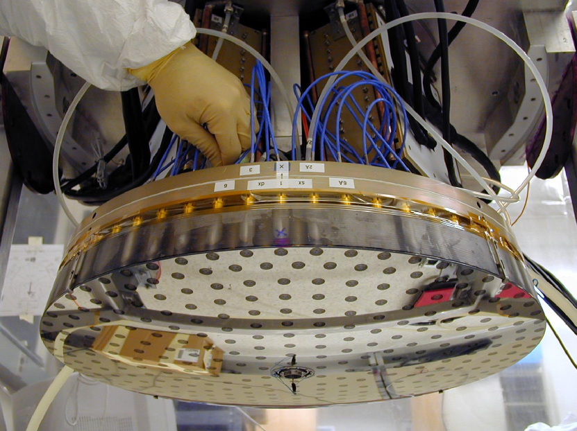
Figure 8.— The MMT’s deformable secondary mirror with an oblique view of the 336 voice coil actuators and their modified hexapolar placement.

The actuators provide non-contact forces to the shell via electromagnetic voice coils acting on magnets attached to its inner surface. The gap between the shell and the reference body is measured by capacitive sensors at each actuator, and is actively maintained by a 40 kHz servo in a dedicated mirror controller. The typical time for the shell to reach a desired position is less than 1 ms.

The MMT AO processing is performed by a real-time Linux computer system (Vaitheeswaran et al., 2008) which reads the WFS camera, computes the required wavefront updates, and sends updated commands to the deformable secondary controller, all synchronously clocked by the WFS frame rate. The 12$\times$12 subaperture Shack-Hartmann WFS (Mcguire et al., 1999) is normally operated at 527 Hz. The AO computer calculates the wavefront slopes, reconstructs an estimate of the wavefront, applies a conservative modal filter, and sends the updated actuator commands to the deformable secondary controller.

The MMT’s Shack-Hartmann WFS uses a $12\times 12$ lenslet array to image the starlight within each subaperture onto the center of a binned $2\times 2$ pixel “quad-cell.” Local wavefront slopes cause the image to shift, changing the relative amount of starlight entering the various quad-cell pixels. The pixels are exposed, read out, summed, differenced, and mapped through a lookup table matched to the seeing level, yielding estimates of the $x$ and $y$ wavefront slopes over each of the 144 subapertures (Hardy, 1998). The pixel sums and differences are normalized by the sum of the quad-cell counts, plus a small bias term. The bias ensures that unilluminated quadcells generate zero slope estimates. The resulting 288 $x$ and $y$ slopes are serialized into a single column vector (the “slopes vector” $\bm{\Theta}$). The AO system estimates the residual wavefront by multiplying the slopes vector with a wavefront reconstructor matrix, $\bm{W}_{AO}$, resulting in an estimate of the residual wavefront error at the actuator positions: $\delta\bm{z}=\bm{W}_{AO}\bm{\Theta}$. An AO reconstructor typically has a combined legacy of optical measurements and analytical processing, characterized ultimately by a number of singular value decomposition (SVD) modes (Brusa et al., 2003). The MMT AO reconstructor uses lowest-energy mechanical modes of the thin shell as a basis set. This restriction means that the wavefront spatial frequencies are not uniformly corrected within the modal control radius of the mirror, implemented as a safety precaution. Subsequent developments with the LBT AO system (Esposito et al., 2010) and Magellan observatories are less constrained. The wavefront correction is post-processed using a “modal filter” to redundantly ensure that damaging stresses are not applied to the shell. Once calculated, the residual wavefront estimates are multiplied by an overall (scalar) gain factor and added to the correction already applied to the mirror. The result is then sent to the mirror controller where it is applied with its own high-speed servo control loop.

There were several issues with the MMT AO system at the time of observation. The gains on individual mirror actuators had not been recalibrated for several years and in some cases had drifted by as much as tens of percent. Thirteen out of the 336 actuators were non-functional (Fig. 9).

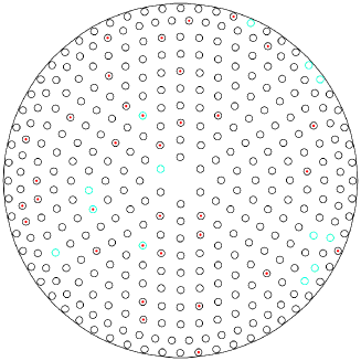
Figure 9.— Locations of the MMT deformable secondary mirror actuators (circles). At the time of our measurements, there were 13 disabled actuators (light gray circles) that float to a point between the adjacent actuators. 34 actuators had problematic or failed capacitive sensors (dots), but were still able to be driven in open loop by the mirror controller. For the 56-mode correction applied by the AO control servo, having 10% failed actuators has only a marginal effect.

The loss of these actuators did not significantly impact low-order correction modes as the DM shell above a deactivated actuator floats to a position interpolating that of its neighbors. Another 34 actuators had inoperative capacitive sensors, requiring their positions to be set in the high-speed mirror controller by dead reckoning rather than using the closed-loop control servo. In addition to some mount vibrations, our observations include significant pointing swings deliberately introduced as a signal for calibration of a pyramid wavefront sensor. These vibrations have amplitudes in excess of 100 mas (i.e. on the order of a science camera image diffraction width).

4.1.2 The Clio mid-infrared Science Camera

Our science camera was the mid-infrared Clio system (Freed et al., 2004; Sivanandam et al., 2006). Light from the deformable secondary directly enters Clio’s dewar through a tilted dichroic window, forming an $f/15$ image at the first focal plane. A re-imaging lens forms another pupil plane, usually for bandpass filters and Lyot stops, but also where Clio’s Apodizing Phase Plate (APP) is located (Kenworthy et al., 2007). A final lens images the pupil plane onto the focal plane imaging sensor. Clio’s sensor is a HAWAII-1 HgCdTe array with 18.5 $\mu$m square pixels cooled to 75.6 K. The detector gain is 4.9 $e^{-}$/dn with a bias of 3700 dn and a saturation level of 55,000 dn, giving a full-well capacity of 51,000 dn (250,000 $e^{-}$). The read noise for a single frame is 19 dn (93 $e^{-}$). The dark current is 50 dn/s (245 $e^{-}$/s) at 75.9 K. Clio’s plate scale was measured as 0.0299”/pixel or 4.0 pixels$/\left(\lambda/D\right)$ in L band. Clio is controlled by a computer running Linux, taking exposures and saving FITS image cubes asynchronously from the AO system. Data is taken using a special 54$\times$108 “sub-stamp mode” to achieve a higher frame rate.

4.2. Synchronizing WFS and Science Data

Since the speckle phases change rapidly, both randomly and in a deterministic way depending on position within the field and the projected speed and direction of the wind, small synchronization errors can cause both random and systematic biases in the measured halo phase. Without taking particular care, we might expect the phase error to be determined by how much the speckle phase changes during the science camera’s exposure time. However, this can be reduced by carefully synchronizing the WFS frames to the start and end of the science frames, thereby achieving phase accuracies more in line with the the speckle phase change during a single WFS frame. This improvement (a factor of 6.5 in this dataset) only helps reduce biases. The loss of coherence caused by the science camera exposure time is not recoverable and still reduces the measurement SNR. However, by removing systematic effects, averaging will still yield more accurate measurements at the higher frame rate.

All AO system updates occur at the WFS frame rate. In an engineering diagnostic mode, the AO host computer buffers 10,000 frames of engineering data into a set of RAM-based circular buffers. Once these buffers are filled, a separate processing thread writes them out to the AO computer’s hard disk. The MMT WFS frames are normally taken at a steady rate, but an engineering issue resulted in every other WFS frame being dropped from the data telemetry, resulting in the system operating at half its normal speed.The result was that the normally 527 frames/s rate was reduced to approximately 263.5 frames/s with a slopes file saved every 38 s. To avoid timing problems and other possible buffer overrun issues, we did not include any science data sets that ran across WFS slopes files. These issues do not impact our technique. Clio buffers 100 contiguous exposures in RAM before saving them to disk. When the RAM-based image buffer is filled, the camera acquisition halts while the images are saved. The non-standard small images were acquired at approximately 40.5 frames/s, filling the 100-image buffer in about 2.5 s and saved to disk every 3 s. Within each Clio data cube, the images are continuous sequential exposures, with each exposure ending as the next began.

Both the AO and Clio control computers run Network Time Protocol (ntp) clients. The resulting filesystem and internal header timestamps are directly compared between computers, allowing us to uniquely associate log entries and data files. Using ntp alone does not guarantee synchronization to the WFS frame level. The AO engineering diagnostics files contain only data and no internal timestamps or other useful FITS header information. The primary identifying information was a unique file name which included a numerical code derived from internal counters and the time of the first frame, recorded to 1 second accuracy. The operating system also encoded timestamps in the filesystem inodes when the file was written. Since these are volatile upon copying and archiving, we saved them to a file after the run using the Linux command “ls -lt --full-time > timestamps.log” which preserved the file creation times in ISO format to the accuracy configured in the kernel (only 1-second accuracy for both systems). The Clio file creation timestamps are also saved as a fallback procedure, but the primary record there was a timestamp saved in the FITS file header.

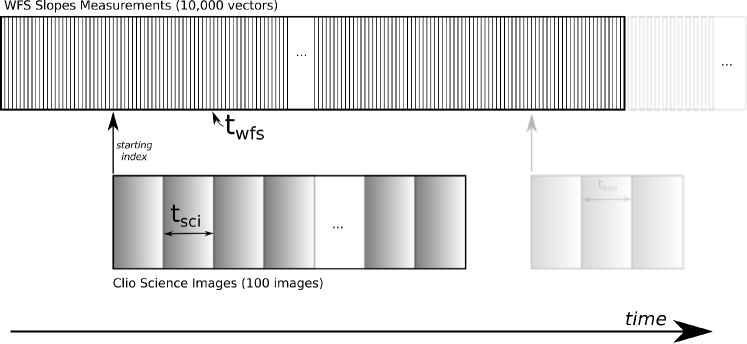
Figure 10.— WFS and science data cubes have asynchronous placement and non-guaranteed timing. Although clock synchronization, network handshaking, timestamps, and logging procedures were implemented, a data-based cross correlation procedure was also required to ensure proper synchronization.

In addition to the timestamps, we implemented a simple network handshaking protocol to record the WFS frame information to higher accuracy. At the beginning of a set of science images, The science camera control computer sends a UDP packet to the AO host computer. Once received by the AO system, this information is written to the AO log file along with the base name of the WFS engineering files currently being recorded and the current WFS frame number. This information is later extracted from the log and used to align the data sets to within a few WFS frames. The handshake procedure contains an unknown delay from the time Clio transmits the UDP packet and the AO system wrote the current WFS frame offset to the log file. This correlation gave us the mean number of WFS frames per science exposure, $\left\langle\mathsf{t}_{sci}/\mathsf{t}_{wfs}\right\rangle$, and the lag between the logged frame number and the correct value.

Using the images from a single 100-frame Clio file, we determined the location of either the star’s peak pixel or its centroid. We then interpolated this time series based on an assumed value for $\left\langle\mathsf{t}_{sci}/\mathsf{t}_{wfs}\right\rangle$ to the WFS frame rate, allowing a cross correlation with the mean $\theta_{x}$ and $\theta_{y}$ time series determined from the appropriate subset of the WFS slope file, extended before and after by a generous set of additional frames. The concurrent engineering tests were introducing a lot of tip-tilt noise, giving us a strong signal for the timing calibration. Our exposures were short enough that this did not cause us any problems. Even so, the normal tip-tilt noise in the AO system would have been adequate for this determination. The science camera and the WFS are not necessarily aligned, but were in this case. Even so, we correlated all four combinations between the two inputs to ensure that we had the coordinate mapping correct. By varying the presumed ratio of frame rates, we determined $\left\langle\mathsf{t}_{sci}/\mathsf{t}_{wfs}\right\rangle\approx 6.48\pm 0.03$. Thus, in 100 continuous science exposures, assuming the center exposure was correctly placed, the start and end exposures have a placement uncertainty of $\pm 1.5$ WFS frames or 5.7 ms. The cross correlation analysis also determined the lag from the handshake protocol to be 3 WFS frames. Once calibrated, the handshake protocol alone was sufficient to synchronize the Clio images with the WFS data to within a WFS frame on the average. Without the random WFS readout timing problems encountered during our test run, and a measured frame rate for the science camera, all the exposures would be placed relative to the WFS with equal precision, and overall accuracy would be determined by the accuracy of the calibrated handshake. This is expected to be within a single WFS frame, which is the limit of accuracy for the system. As we shall see below, the speckle coherence time varies across the field, but the minimum values are comparable to the timing accuracy errors at the bounds of the exposures. The result is that there were some coherence losses in SNR due to temporal misalignment between the datasets, but they were not serious enough to limit our results.

4.3. Science Camera PSFs

The observed star is a 7.4 mag G5 star at zenithal angles ranging from 13 to 14 degrees (Fig. 11).

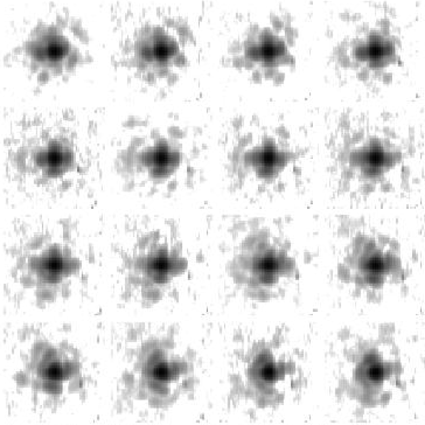
Figure 11.— Clio star images. These 16 sequential images are shown with a 3 decade log grayscale.

Clio was configured for direct imaging with a Barr MKO L’ band filter (Tokunaga et al., 2002), centered at 3.8 $\mu$m and a bandpass of 0.7 $\mu$m. At the center wavelength, the Clio pixels subtend $\lambda/4.0D$. The $54\times 54$ pixel region readout from the sensor was calibrated with dark and flat images, with noisy or bad pixels flagged and replaced by the median of a $3\times 3$ window centered on the pixel. Image vibrations were removed by shifting the PSF center with bilinear interpolation to a fixed location. The PSF peak was located using correlation with a Gaussian reference peak. The pointing vibration during our observations had a swing of approximately 1.5 – 2 $\lambda/D$ which contributed only a small amount of image motion blur during any given Clio exposure. This vibration did not significantly impact the data reduction process, but did have the effect of dithering over any bad pixels, reducing their influence. It was not possible to precisely know at observation time where we were in the WFS buffer, so no attempt was made to avoid the times bridging slopes files. To avoid any possible timing complexities, any Clio image cubes that bridged WFS file boundaries were simply discarded.

4.4. Complex Speckles from WFS slopes

We first use the WFS measurements to estimate the varying wavefront displacement in the pupil plane $z(\mathit{\mathbf{x}},t)$, where $\mathit{\mathbf{x}}$ is the position in the pupil plane. Using the science camera filter band’s mean wavelength $\lambda$, we compute the phase shift caused by the displacement, $\varphi(\mathit{\mathbf{x}},t)=kz(\mathit{\mathbf{x}},t)$, where $k=2\pi/\lambda$. Ignoring scintillation, we write a unit amplitude complex field in the pupil plane as $\exp\left\{i\varphi(\mathit{\mathbf{x}},t)\right\}$, pass it through the pupil stop $\Pi(\mathit{\mathbf{x}})$, and then use Fourier optics (Goodman, 1995) to find the complex halo in the image plane

$$\Psi(\bm{\kappa},t)=\int e^{i\bm{\kappa}\cdot\mathit{\mathbf{x}}}e^{i\varphi(\mathit{\mathbf{x}},t)}\Pi(\mathit{\mathbf{x}})\,\mathrm{d}^{2}x$$ (40)

where $\bm{\kappa}$ is spatial frequency in the pupil plane and $\bm{\theta}=\bm{\kappa}/k$ is the corresponding angular coordinate (in radians) measured from the star. Over a given observation period, we can make a distinction between the “static halo” and “speckles” as

$$\Psi(\bm{\kappa},t)=\underbrace{\overline{\Psi}(\bm{\kappa})}_{static\,halo}+\underbrace{\psi(\bm{\kappa},t)}_{"speckles"}.$$ (41)

(A more detailed discussion of the separation of the halo into its static and speckled components is given in App. A.) Basic Fourier optics is a very simple model for an imaging system, with no place to properly introduce aberrations that occur after the starlight passes the pupil without significantly increasing the complexity of the optical wave model. Aberrations that occur anywhere other than the pupil plane (or images thereof), will affect the halo and speckles differently depending on where the star appears in the camera’s field of view. Since the field of interest in high-contrast imaging is very small, we only introduce negligible errors by treating all aberrations as having taken place in the entrance pupil plane, including any downstream aberrations not seen by the AO system (i.e. NCP aberrations). It is because of this that we may measure the complex halo in the focal plane and then use Fourier optics to find an equivalent distorted field in the pupil plane. Since we do not know the NCP aberrations a priori, we must compute the speckle halo without them. Depending on the magnitude and nature of the NCP errors, this can have a large effect, distorting both the static and speckle halos. At higher Strehl ratios (where the peak of the diffraction-limited PSF is much brighter than the speckles), each individual complex speckle can be thought of as a translated, scaled, and phase-shifted copy of the speckle-free halo. Therefore, including the NCP aberrations would mostly just alter the “speckles on the speckles”, adding noise to the speckle halo, but having only a minor effect on the brighter speckle peaks. The NCP errors also alter the static halo, often in ways which cannot be ignored. However, by estimating and removing the idealized static halo from our calculation, we are left with just the speckles. This justifies why we can ignore the NCP aberrations when computing the speckles, allowing us to bootstrap our interferometric measurement of the true static halo. If we need more accuracy, we can iterate the process by using the first estimate of the NCP aberrations in a second calculation of the complex speckle halo.

As we collect WFS data, we repeatedly carry out the above steps to build a “data cube” of complex halos that do not include the effects of NCP errors, but do include residual AO speckles along with a simplified static halo. This static halo is presumed common to all frames of the data cube ($\Psi_{nmw}\equiv\Psi(k\bm{\theta}_{nm},t_{\mathit{w}})$, where $\bm{\theta}_{nm}$ is the grid of pixel coordinates) and can be estimated by averaging over the time index. Since we force the time average of the speckles to be zero over each data cube, we are actually pushing any estimation error onto the derived static halo. This is a consequence of processing with smaller data cubes, and the resulting individual static halo estimates from multiple data cubes, when averaged, should lead to a more accurate answer.

As mentioned earlier, the WFS slopes are related to wavefront displacements by a “reconstructor matrix.” This is essentially an integrator, working on the set of $x$ and $y$ slopes returned from the WFS sub apertures. The $x$ and $y$ slopes from the $12\times 12$ WFS are serialized into a single $288\times 1$ “slopes vector”, $\bm{\Theta}$, which is integrated into a wavefront by multiplying by a “reconstructor matrix” $\bm{W}$: $\bm{z}=\bm{W}\bm{\Theta}$. Since the MMT AO wavefront reconstructor, $\bm{W}_{AO}$, only corrects a limited number of modes (currently 56), it is not sufficient for our complex halo calculation. If we consider each pair of modes to be the equivalent of controlling the real and imaginary parts of the complex amplitude of a speckle, each of which has a width of roughly $\lambda/D$, then 56 modes will take us out to roughly $3.7\lambda/D$ from the star, while the WFS is capable of at least $6\lambda/D$. To allow us to properly recover the residual wavefront to the accuracy of the WFS rather than being limited by the AO system, we require a better reconstructor, $\bm{W}_{residual}$. Since our reconstructor is not used to drive the DM, nor is it intended to be iterated by being placed inside of an AO servo loop, it is not as important to be conservative about issues such as modal gain, making it easier to derive an adequate reconstructor. Also, since the computed displacements are not going to be used to drive the actual DM, we can choose to reconstruct the wavefront at more conveniently-placed locations across the pupil: e.g. on a square grid, instead of the actual hexapolar locations of the physical DM. But here, to facilitate direct comparison with the AO system’s data as well as other live reconstructor tests, we used the physical actuator locations. For each WFS slopes vector, the estimated residual wavefront displacements at the actuators are given by $\bm{z}=\bm{W}_{residual}\bm{\Theta}$.

We estimated and removed the mean $x$ and $y$ slopes from the slopes vector before multiplying by $\bm{W}_{residual}$, resulting in a vector of wavefront displacements with tip-tilt removed. For computing the complex pupil field and halo, we interpolated the wavefront displacement estimates at the actuators to a 4 cm square grid using Delauney triangularization and cubic interpolation, yielding a wavefront displacement $z_{nm}$ at $\mathit{\mathbf{x}}_{nm}=(n,m)\delta x+\mathit{\mathbf{x}}_{00}$. The complex pupil field was computed by $\Upsilon_{nm}=\Pi_{nm}\exp\left(2\pi iz_{nm}/\lambda_{science}\right)$, where $\Pi_{nm}$ is the pupil transmission mask interpolated to the grid coordinates. The resulting complex mesh was zero-padded to $N\times N$ and Fourier transformed, giving focal plane samples spaced by $\delta\kappa=2\pi/N\delta x$ and angular spacing of $\delta\theta=\lambda_{science}/N\delta x$. We adjusted $N$ to match the L-band Clio plate scale of $0.25\lambda/D$. The focal plane field was computed using 2-D FFTs and the results kept in a complex data cube $\Psi_{nmw}\equiv\Psi(\kappa_{x},\kappa_{y},t_{\mathit{wfs}})$. This processing was performed for each set of 100 science camera images ($\sim 2.5$ s), with the corresponding set of WFS frames selected and used to compute a halo data cube spanning the science camera exposures at the WFS frame rate. Since the synchronization between the WFS data and the science camera is only accurate to about one frame from the center of a 100-exposure image set, but the duration of the individual exposures is 6.5 frames, the starting frame index is assumed to be on a frame boundary, with subsequent exposures placed on the timeline as they fell. The full-speed complex halo was then down-sampled to the science camera frame rate by summing the complex frames, including linearly-weighted end frames according to the computed endpoints. Finally, since the actual piston and tip-tilt may have changed during a single science camera exposure, we performed the complex halo sums before normalizing to the peak phase. Since tip-tilt was removed in the slopes before computing the halo, motion blur was not fully represented, but the image wander is much smaller than $\lambda/D$ during any single science camera exposure and the error introduced is small. The complex halo estimate at the science frame rate was

$$\widehat{\Psi}_{nm\mu}=e^{-ip_{\mu}}\sum_{w\in\mathsf{t}_{sci}(\mu)}\Psi_{nmw}$$ (42)

where $p_{\mu}=\left.\arg\left\{\sum_{w\in\mathsf{t}_{sci}(\mu)}\Psi_{nmw}\right\}\right|_{core}$. Since $\left\langle\phi\right\rangle=0\nRightarrow\arg\left\{\left\langle e^{i\phi}\right\rangle\right\}=0$, core phase referencing was performed on the complex WFS PSF halo.

Since the individual complex halo cubes were so short, we did not force the mean speckle field to be zero for each individual cube, giving a changing estimate for the simplified static field used in the calculation. Instead, we used an estimate of the ensemble average of the halo, (i.e. $\mathscr{S}^{1/2}\Psi_{0}$ as described in App. A) and used it to estimate the speckle halo over each cube. This is better than using the per-cube average since the estimation error appears as a constant across the pupil rather than randomly textured (Sec. 4.6). Our resulting speckle field was

$$\psi_{nm\mu}=\widehat{\Psi}_{nm\mu}-\mathscr{S}^{1/2}\Psi_{0}.$$ (43)

Note that while this is no longer zero mean on the scale of individual image cubes, it should approach zero mean in the ergodic limit of many data cubes. The speckle field is now able to be directly compared with the science camera image cubes as they are synchronized and have the same sampling in space and time.

Before continuing on to compute the static halo, it is useful to look at the behavior of the complex speckles and their spatial and temporal statistics to understand how our result is affected by exposure time, wind, etc. Fig. 12 shows an angle-time cut through the center of the speckle field in the projected direction of the wind to illustrate the lifespan of the speckles, with both amplitude and phase variations.

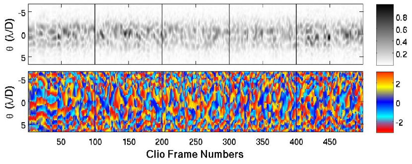
Figure 12.— A cut through the computed speckle field for five non-contiguous Clio image sets. The upper panel shows the speckle amplitudes as a function of time while the lower panel is the speckle phase relative to the light in the PSF core. The 100 Clio frames of each set are contiguous, but not across boundaries at multiples of 100. The speckle amplitudes are arbitrarily normalized to the brightest value.

The speckle amplitude variation timescale is reasonably consistent across the speckle cloud, while the speckle phase has a similar pattern superimposed on a steady phase rate that increases as we move away from the star. These speckles coherently add to the as-yet unknown static halo, the intensity being recorded by the science camera. We can make a visual comparison of the science images frame-by-frame to the WFS-based images using $\left|\widehat{\Psi}_{nm\mu}\right|^{2}$, which is based on our simplified no-NCP error model (Fig. 13). This figure illustrates if we are indeed computing speckles when and where they were actually observed, and the extent of any deviations.

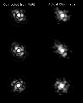
Figure 13.— Star images computed from the residual WFS measurements (left column) alongside the corresponding Clio images (right). The computed images mainly differ from the actual images in optical bandwidth and non-common-path (NCP) aberrations. The computed images are monochromatic and assume that the estimated wavefront seen by the WFS is the only source of aberration.

For each row in Fig. 13, the PSF derived from the WFS slopes is shown on the left, while the corresponding Clio image is on the right. The two images exhibit similar behavior, but with the single-wavelength computed PSF having more well-defined speckles than the actual science images due to the bandwidth of the science images. The speckles in the computed images may also be more or less prominent than the real images since the reconstructor gain may be incorrect as a function of position around the star (i.e. a possibly incorrect modal gain). Also, since NCP aberrations and low-order effects such as defocus are not included in the computed PSFs, there might be noticeable differences between computed and real images, as well as complicated differences with the speckles. In our present case the comparison is reasonably good, providing a sanity check that the synchronization and WFS-to-speckle calculation was performed correctly.

The various statistics are straightforward to compute from the image and complex speckle data cubes. The intensity variance is

$$\sigma_{I}^{2}=\frac{1}{N}\sum_{w=1}^{N}\left(I_{nmw}-\frac{1}{N}\sum_{w^{\prime}=1}^{N}I_{nmw^{\prime}}\right)^{2};$$ (44)

the mean speckle halo intensity is

$$\Phi_{speckles}=\frac{1}{N}\sum_{w=1}^{N}\left|\psi_{nmw}\right|^{2};$$ (45)

the variance in the speckle halo’s intensity

$$\sigma_{speckles}^{2}=\frac{1}{N}\sum_{w=1}^{N}\left(\left|\psi_{nmw}\right|^{2}-\Phi_{speckles,nm}\right)^{2};$$ (46)

and the stabilized intensity is

$$\left\langle\psi I\right\rangle=\frac{1}{N}\sum_{w=1}^{N}\psi_{nmw}I_{nmw}.$$ (47)

The scale factor $\mathit{g}$ is computed using Eq. 26 and the static halo $\Psi$ is given by Eq. 27.

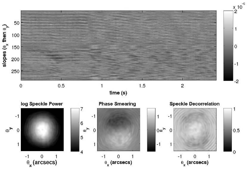
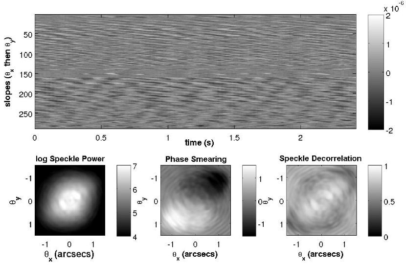
Figure 14.— The effect of wind speed on the distribution and evolution of the speckles. Two 2.5 s WFS data sets are shown, with the 2.5 s of WFS slopes vectors organized as a $288\times 650$ matrix. The slopes were reconstructed into residual wavefronts and used to compute the complex speckle halo. In the top set of images the wind is slower, while in the lower set the wind is gusting to more than twice the upper speed. The speckle halo’s mean intensity is shown on the left. The slower wind case is dominated by the relatively isotropic fitting error, while the faster wind shows a prominent lag error speckle plume in the (shifted) direction of the wind. The average speckle intensity is shown using a square root scale. The systematic phase smearing during a Clio exposure is is shown in the center image. Finally, the speckle decorrelation on the right shows the loss of speckle coherence at a lag roughly equal a Clio exposure.

The wind speed gusted by more than a factor of 2 and changed direction by more than 45 degrees during the observation, causing clearly-visible effects in the speckle field statistics. When the wind was slower (say 5–10 m/s), the speckle cloud was more isotropic with a form characteristic of fitting error, while stronger wind gusts enhanced the plume of lag-error speckles. Fig. 14 shows two selected times with slower and faster wind. For each case the figure shows the WFS slopes and three derived speckle statistics. The $12\times 12$ sub-aperture Shack-Hartmann WFS slopes were organized into 288-element vectors and concatenated into a matrix of slopes (upper images). The speckle halo was computed for each slopes vector and the three statistical images were averaged from the 650 complex speckle frames. The lower left images are the average speckle power centered on the star, showing the morphological change between the more isotropic fitting error halo and the lag error speckle plume. The middle image is the average amount of phase rotation seen during a Clio exposure, computed from the two-time MCF (Eq. 35): $\delta\phi(\bm{\theta},\mathsf{t}_{sci})=\arg\left\{\Gamma(\bm{\theta},\mathsf{t}_{sci})\right\}$. The phase rotation is mostly a systematic translation effect, while the loss of coherence due to random effects is better described by the drop in the magnitude of the MCF $\left|\Gamma(\bm{\theta},\tau)/\Gamma(\bm{\theta},0)\right|$, shown in the lower right images in Fig. 14 for a lag of $6\,\mathsf{t}_{wfs}$. The linear grayscale runs from completely incoherent (black) to completely coherent (white). The results show that while fitting error speckles rapidly lose coherence, lag error speckles remain coherent longer in the direction of the wind. This is due to the well-known phenomenon of the AO system repeatedly making the same lag-induced correction error as the aberrations are carried across the pupil.

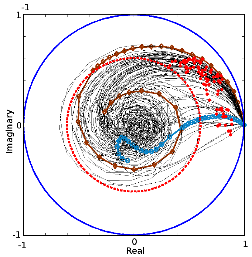
Figure 15.— Normalized mutual coherence function $\Gamma(\tau)/\Gamma(0)$ for a single point in the second Airy ring. Two example cases are highlighted, one where the angle between the wind vector and the pixel vector is small, (brown with diamonds) and one where the angle is significantly larger (blue with circles). For each of the WFS-derived speckle data cubes, $\Gamma(\tau)$ was computed at lags $\tau:\{0,1,2,\cdots,20,25,30,\cdots,100\}\mathsf{t}_{wfs}$. The speckles always decorrelate with time, but wind causes a systematic phase shift in a direction related to the projection of the wind on the selected point in the focal plane. The interesting cases where the angle swerves from one sign to the other are caused by more than one wind stream competing. The values of the MCF at the end of the Clio exposure are shown as filled red circles, showing that for this pixel the phase smearing was never a serious issue. The speckle coherence time, $\tau_{0}$, is defined as when $\Gamma(\tau)/\Gamma(0)$ crosses the red dashed circle at a radius of $e^{-1/2}$. The more wind-blown lag error speckles remain coherent longer since the AO system repeats the same error as the wind carries the aberrations across the pupil. This function and its two main behaviors (straight decorrelation and systematic phase shift, see Eq. 38) determine the loss of SNR for various science camera exposure times (see Sec. 3.1).

A more quantitative view of the speckle evolution and decorrelation is shown in Fig. 15. As described by Eq. 38, part of the MCF describes the speckles’ decorrelation, while a phasor factor systematically rotates the phase depending on the wind’s projection onto the selected point’s position relative to the star. The figure shows the MCFs, normalized by the zero-lag value (note $\Gamma(0;\bm{\theta})=\Phi_{speckles}(k\bm{\theta})$), for a single selected point in the second Airy ring for all of our speckle data cubes. This complex function shows the speckle decorrelation as a decrease in the absolute value of $\Gamma(\tau)$ with increasing time, as well as the systematic phase rotation caused by the wind. But also, the figure shows that when the wind is faster, the MCF falls in magnitude much more slowly. This is due to the AO system repeating the same error as it “chases” the wind-driven aberrations across the pupil. While this effect increases speckle noise due to fewer statistically-independent speckles in a given exposure, it helps us in that longer-lived speckles can be imaged with more modest science camera frame rates, like 30 fps. Both speckle decorrelation and phase rotation affect our interferometric measurement’s SNR, as we will see below.

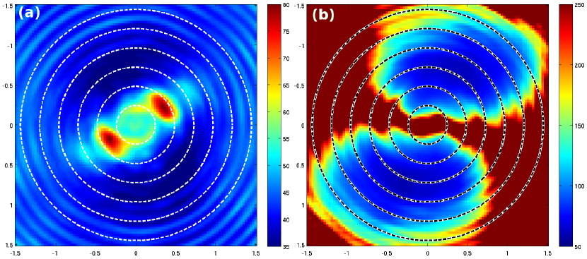
Figure 16.— Average speckle halo characteristic timescales across the focal plane (dashed circles at $1\lambda/D$ spacings). The wind-driven speckle plume varied about a direction roughly 60 degrees clockwise from the positive y-axis. Image (a) is the characteristic coherence time computed using $\left|\Gamma(\tau)/\Gamma(0)\right|=e^{-1/2}$. The color scale is labeled in milliseconds and runs from 35 ms to 90 ms. The fitting error speckles typically decorrelated after 35–50 ms while the lag error speckles in the apparent direction of the wind lasted longer. Note that the lag-error speckle lifetimes were longer when they appeared over an Airy ring, which was not expected. Image (b) shows the average time required for the speckle phase to change by $\pm\pi/2$, extrapolated from the phase swing after 4 WFS frames. The color scale runs from 50 to 250 ms.

In the pre-AO pupil plane, the coherence time is usually defined in terms of advection of the wavefront by pure Taylor flow. This implies that the natural definition of coherence time is $D_{\phi}(\mathbf{v}_{wind}\tau_{0})=1$, or as is often quoted, $\tau_{0}=0.314r_{0}/\mathbf{v}_{wind}$ for a Kolmogorov wavefront (Greenwood & Fried, 1976). However, this is more properly defined in terms of the temporal MCF, $\Gamma(\tau)=\left\langle\psi(\mathit{\mathbf{x}}+\mathbf{v}_{wind}\tau)\psi^{*}(\mathit{\mathbf{x}})\right\rangle=\exp\left\{-D_{\phi}\left(\mathbf{v}_{wind}\tau\right)/2\right\}$, where the canonical structure function definition becomes $\left|\Gamma(\tau_{0})/\Gamma(0)\right|=e^{-1/2}$. This is the definition we used to compute the focal plane coherence time in Fig. 16(a). Note that the coherence time is only about 35–50 ms except in the speckle plume where the coherence time is much longer. This is the expected behavior with a non-predictive AO servo algorithm that uses only the most recent WFS measurements to update the DM. It is interesting to note in Fig. 16(a) that the lag-error speckle coherence time is longer over the Airy rings. This was not expected, but may be due to the wind bringing in unseen aberrations at the edge of the pupil. More study is required.

The other timescale of concern is how long it takes for the systematic phase shift to change by $\pi/2$, after which at least some of the interferometric reference beam contributions will start to subtract. Note that outside of the speckle plume, the phase shift timescale is longer due to the oblique translation geometry or irrelevant due to the lack of persistent speckles. For speckles that are more in-line with the wind flow, the phase change becomes more consistent and the lag error speckle plume makes the effect dominant. For our data set however, the most important effect over the majority of the focal plane is the changing residual aberration pattern, not the translation by the wind.

The most useful and practical metric is the additional loss of SNR due to longer science camera exposures. As expressed in Eq. 37, the SNR is reduced by a weighted integral over the MCF at various lags. This can be computed from our WFS data and is shown in Fig. 17.

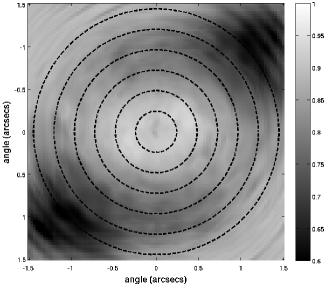
Figure 17.— The pixel-by-pixel worst-case loss of SNR due to science camera exposure time, compared to an ideal short-exposure SNR. The Clio exposures were 6.5 times longer than the WFS exposures, so there was some loss of SNR depending on the wind and focal plane position. The SNR was only down to about 90% nearer to the star, dropping to about 60% in the processing-lag speckle plume as the phase wrapping rate increased farther from the star. For this bright star and weather circumstances, we would have no difficulty analyzing low-order aberrations with even significantly longer exposures.

The figure shows that although the Clio exposure times were long enough to show a great deal of coherence loss end-to-end, the SNR dropped to only about 60% to 90% of an arbitrarily high frame rate camera. This can be recovered everywhere, if required, by integrating about 3 times longer.

In each of these figures, there are occasional resonant speckles caused by processing lag and wind, along with the particular characteristics of the reconstructor, lead to enhanced speckles at certain angles. This was an unusual situation, possibly due to the engineering tests being performed. However, such phenomena can occur in a live AO system and may cause difficulties in the measurement. In this case, the speckle phase distribution about the mean was still sufficient to give a good statistical measurement of the static halo. But they are certainly a sign that greater care should be taken.

4.5. Estimating the static halo

As derived in Sec. 2.2, we can estimate the static halo from the Clio and complex speckle data cubes using Eq. 27. In discrete form this is

$$\overline{\Psi}_{nm}=\frac{\sum_{w}\psi_{nmw}I_{nmw}}{g_{nm}\sum_{w}\left|\psi_{nmw}\right|^{2}}.$$ (48)

The scale factor is a function of position and is computed using Eq. 26, shown in Fig. 18. As expected for a reconstructor that is not carefully calibrated, the speckles do not have a uniform scale over the working field.

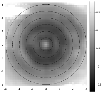
Figure 18.— Map of the scale factor $g(\bm{\theta})$ in a neighborhood around the star. The scale is base-10 log and the circles are 1–6 $\lambda/D$. The white area on the upper left is due to a dithered flaw in the sensor.

Including this correction, we now have an estimate of the static complex halo as shown in Fig. 19.

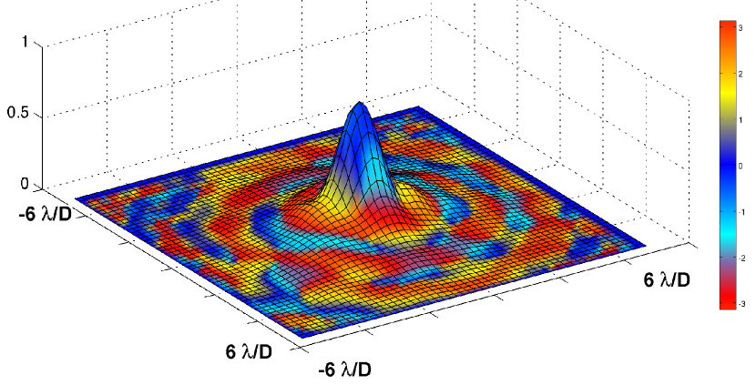
Figure 19.— Average complex halo derived from 67 2.5 s Clio image cubes (6700 images) and 43,550 WFS measurements. This calculation used the presumed ensemble average method for computing the speckles and therefore may be missing an additive fraction of the ideal complex halo.

Armed with this information, we can now use it in an anti-halo servo to suppress the halo over some region of interest (Codona & Angel, 2004), or we can use the entire halo to estimate the wavefront in the pupil plane including the NCP error to improve the Strehl ratio and imaging quality at the science camera. This use of the measured static halo requires more work but is conceptually as simple as taking the Fourier transform of the static halo.

4.6. Estimating the pupil field

The static halo is the mean of the complex halo (App. A, specifically Eq. A1), and therefore it is the inverse Fourier transform of the mean complex pupil field $\Upsilon(\mathit{\mathbf{x}},t)$ under the paradigm of Fourier optics (Eq. A22). Our static halo field includes the effects of any non-common-path aberrations after the AO system and the science camera, which may have been introduced at any point in the intervening light path. The inverse Fourier transform of the static halo does not give the literal pupil field, but the apparent pupil field including the effects of the downstream aberrations back-projected to the pupil. Since the pupil is the canonical location of the DM where we can affect wavefront corrections, we can use this estimate to determine the wavefront offsets required to modify the resulting halo in any desired way. Expressing this in terms of the forward Fourier optics equation, Eq. 40, we write

$$\Upsilon_{0}(\mathit{\mathbf{x}})\Pi(\mathit{\mathbf{x}})=\frac{\int e^{-i\bm{\kappa}\cdot\mathit{\mathbf{x}}}\overline{\Psi}(\bm{\kappa})\mathrm{d}^{2}\kappa}{\left(2\pi\right)^{2}\mathscr{S}^{1/2}}$$ (49)

where we have made use of the assumption that the residual wavefront phase from the AO correction is a zero-mean Gaussian random variable and $\left\langle\exp(i\phi)\right\rangle=\exp(-\left\langle\phi^{2}\right\rangle/2)\equiv\mathscr{S}^{1/2}$ is the square root of the Strehl ratio. This gives us an estimate of the pupil field, blurred due to the limited spatial frequencies recovered by the interferometry calculation. The NCP pupil field is $\bar{\psi}(\mathit{\mathbf{x}})=a(\mathit{\mathbf{x}})\exp\left(ik\delta z\right)$ where the amplitude $a(\mathit{\mathbf{x}})\in\mathbb{R}$ may include transmission effects, as well as back-projections of downstream vignetting, etc. The wavefront to be corrected is given by

$$\delta z=\frac{\lambda}{2\pi}\arg\left\{\int e^{-i\bm{\kappa}\cdot\mathit{\mathbf{x}}}\overline{\Psi}(\bm{\kappa})\mathrm{d}^{2}\kappa\right\}.$$ (50)

This simple procedure should be all that is required to compute the wavefront correction, but there are some caveats and corrections. The pupil field estimate is missing some low spatial frequency components, mostly a constant. The reasons for this have already been discussed in Sec. 3, and are related to our computed phase referencing to the PSF core, and the fact out tip-tilt stabilization reducing the apparent effect of anti-Hermitian speckle pairs near the optical axis. We also did not account for interference between the very low spatial frequency speckle pairs, causing an error that becomes significant within $\lambda/2D$ of the PSF core. We can calibrate this error by applying a known bias to the DM and seeing what the measured value is. Since a constant bias would affect the measured phase aberration according to

$$\widehat{\delta z}=\frac{\lambda}{2\pi}\arg\left\{\psi_{bias}+\int e^{-i\bm{\kappa}\cdot\mathit{\mathbf{x}}}\overline{\Psi}(\bm{\kappa})\mathrm{d}^{2}\kappa\right\}$$ (51)

we can then adjust the constant $\psi_{bias}$ to give a reasonable estimate of the actual aberration.

Since we did not have a calibration for the data presented in this paper, we estimated a constant pupil field of 50% of the mean computed value. Adding this to the computed value for each 2.5 s Clio data cube, we compute the NCP aberrations. A selected subset of the wavefront errors are shown in Fig. 20.

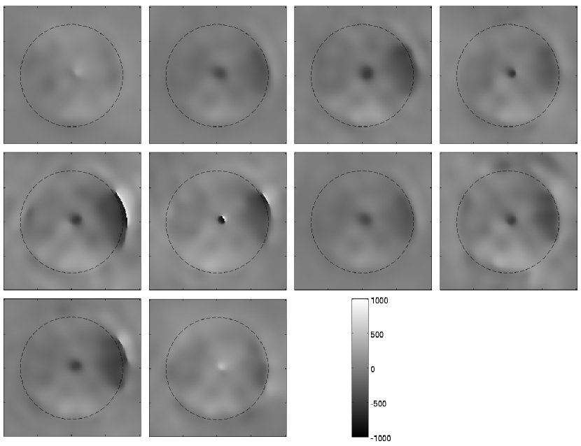
Figure 20.— Examples of 2.5 s estimates of the pupil wavefront. The scale factor $g(\bm{\theta})$ was computed from the full set of 67 100-exposure image cubes and used in the calculation of the static halo for each cube. The loss of low spatial frequency power due to the inability to sense piston as well as tip-tilt stabilization was approximately compensated for by adding a constant to the computed pupil field. The resulting phase was converted to mirror surface heights using $z=\phi(\mathit{\mathbf{x}})\lambda/4\pi.$ The scale is labeled in nanometers.

Since the estimates are generated from only 2.5 s duration science camera cubes, the recovered NCPs show a significant amount of variance, but they also show consistent morphological patterns. The average of these is shown in Fig. 21.

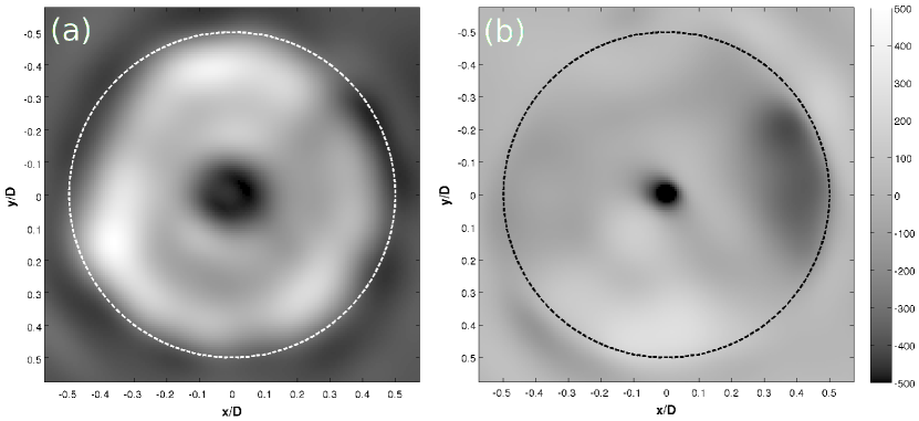
Figure 21.— The MMT’s average static pupil field including back-projected non-common-path aberrations. The pupil field was biased by a constant of 1/2 the rms amplitude to approximately compensate for underestimated low-spatial-frequency power. Image (a) is the intensity, and the $0.1D$ central obstruction is clearly seen. Image (b) is the average WFE computed as a bias to be applied to the DM. The scale is labeled in nanometers. The peak-to-valley surface error is 1266 nm and the rms error is 206 nm (an rms phase error of $\lambda/9.2$ at L band).

The peak-to-valley surface error (i.e. half the wavefront error) is 1266 nm and the rms error is 206 nm. This result is compatible with the science images, and all that remains is to apply the corrections to the DM and see the improvement in the image quality.

5. Discussion

We have developed a new interferometric technique for focal plane wavefront sensing using the residual starlight speckles left behind by an AO system. Our method requires no extra hardware or optics beyond that used in a typical AO system. The rapidly-changing residual AO speckles are present in the science camera image plane and coherently interfere with the starlight diffraction halo. The speckles result from uncontrolled errors in the correction of the atmospheric aberrations, resulting in small residual wavefront fluctuations in a pupil plane downstream from the AO system’s deformable mirror (DM). While uncontrolled and unsuppressed by the AO system, these residual errors are still monitored by the wavefront sensor and are available for other purposes. Improved AO technology and algorithms will continually reduce the errors and subsequent speckles, but they will remain a ubiquitous feature that can be exploited for other purposes. Our technique uses the wavefront sensor measurements to compute a numerical analogue of the complex halo (with both amplitude and phase), which is also measured in intensity by the science camera. The computed halo is used as a key to interpret short-exposure science camera images, allowing the steady portion of the star’s complex halo. Since the intensity measurements are downstream from the AO system, the our complex halo measurement includes information about both common and non-common-path aberrations. This information is useful both for correcting the wavefront before imaging and post-detection image processing.

We demonstrated the technique using data taken with the MMT AO wavefront sensor (WFS) and the Clio science camera in the L band. We synchronized and down-sampled the WFS measurements to match the Clio frame rate of about 40 frames per second. Using our mathematical theory, we were able to compute an estimate of the complex halo every 2.5 s from 100 Clio images and 650 WFS measurements. The resulting complex halo estimate represents the average field in the focal plane and is related to the pupil field by Fourier transform. We analyzed the temporal statistics of the speckle halo and used them to estimate the effect of slower science camera exposures. We found that the impact of exposure time, while depending on the details of wind and focal plane position, was not serious—especially near the star where halo suppression will be most important.

Although we were not able at this time to demonstrate the use of the complex halo to improve the science images, the path forward and potential benefits of continuous end-to-end optical quality measurements and updating are clear. The Fourier transform of the halo provides an estimate of the pupil field, including the back-propagated effects of NCP aberrations. By applying appropriate DM offsets to compensate for the static pupil field’s phase, the Strehl ratio seen by the science camera can be improved, providing correspondingly improved detection sensitivity. Measurements of the complex halo are even more directly useful for suppressing residual diffracted starlight in a flawed or poorly-aligned coronagraph by using an antihalo servo, the theory of which was not discussed in this paper.

In future work we plan on developing a system to estimate the static halo in real time during observations. The estimates will then be fed back to the AO system either as WFS or DM biases. For normal (non-coronagraphic) imaging, the goal will be to optimize Strehl ratio at the science camera. When using a coronagraph, our goal will be to suppress unwanted halo in the search region while simultaneously maximizing Strehl ratio. These enhancements will not require the addition of any new optics, but will require the addition of an outer control loop that affects the operation of the AO system. We also plan to use the complex halo measurements to develop two new image processing algorithms. By using the estimated pupil field, we can compute better numerical PSFs, which include the effects of both common and non-common-path aberrations as well as optical filter bandwidth. Subtracting the computed PSFs from the actual star images will reduce speckle noise. We also plan to use the computed PSFs as a key for when to keep pixels in the science data cube, including them only when the computed halo falls below some statistical threshold. This “lucky pixel” type algorithm should be capable of increasing sensitivity by a factor of about 2. Including both algorithms, the decrease in speckle noise can be significant, depending on the raw performance of the AO system. For the MMT, we would be hoping to achieve an additional sensitivity of 2–4 magnitudes over the corrected coronagraph alone.

Appendix A The static halo and speckle cloud

We treat residual AO speckles to be additive random field fluctuations coherently interfering with a static diffraction pattern. In this appendix we explore the halo, and consider assumptions and statistics. We show why the high Strehl ratio focal plane field is a somewhat attenuated version of the telescope’s diffraction pattern, including non-common-path aberrations, and a coherent cloud of speckles which are reasonably described as zero-mean Gaussian complex field fluctuations. We will consider two cases: the classic seeing-limited situation with no AO wavefront correction as a touchstone, and the diffraction-limited case with a static PSF surrounded by a cloud of speckles.

We start with an incident field $\Upsilon(\mathit{\mathbf{x}})$ passing through a possibly complex pupil mask $\Pi(\mathit{\mathbf{x}})$, which also includes any non-common-path (NCP) aberrations. We will not include scintillation here, but could easily do so. For convenience and wavelength independence, we use the spatial frequency $\bm{\kappa}=(\kappa_{x},\kappa_{y})$ to describe the complex halo field

$$\Psi(\bm{\kappa},t)=\int e^{i\bm{\kappa}\cdot\mathit{\mathbf{x}}}\Upsilon(\mathit{\mathbf{x}})\Pi(\mathit{\mathbf{x}})\mathrm{d}^{2}x$$ (A1)

where

$$\Upsilon(\mathit{\mathbf{x}})=e^{i\varphi(\mathit{\mathbf{x}},t)}\Upsilon_{0}(\mathit{\mathbf{x}})$$

is the pupil field and $\Upsilon_{0}(\mathit{\mathbf{x}})$ is the pupil field without any of the fluctuating phase aberrations $\varphi(\mathit{\mathbf{x}},t)$. Note that our halo field is the angular spectrum of plane waves comprising the pupil field, where each $\bm{\kappa}$ plane wave travels from the direction $\bm{\theta}=\bm{\kappa}/k$ with $k=2\pi/\lambda$. The point spread function (PSF) is the focal plane intensity distribution resulting from an on-axis star, where $\Upsilon_{0}(\mathit{\mathbf{x}})=1$. Although non-common-path aberrations occur downstream from the AO system and the nominal pupil plane, our small field of interest allows us to treat them as being included in the initial pupil field $\Upsilon_{0}(\mathit{\mathbf{x}})$. In our notation, the PSF is the angular power spectrum of plane waves

$$\Phi(\bm{\kappa},t)=\left|\Psi(\bm{\kappa},t)\right|^{2}.$$ (A2)

The fluctuating phase aberrations are presumed to vary randomly in space and time, with ergodicity allowing us to use ensemble and temporal averages interchangeably. While this may be a reasonable assumption for the atmospherically-distorted incident field, it is wise to keep an open mind regarding the post-AO statistics. In general, the average PSF is

$$\left\langle\Phi(\kappa)\right\rangle=\int\mathrm{d}^{2}x_{1}\int\mathrm{d}^{2}x_{2}e^{i\bm{\kappa}\cdot(\mathit{\mathbf{x}}_{1}-\mathit{\mathbf{x}}_{2})}\left\langle e^{i(\varphi(\mathit{\mathbf{x}}_{1},t)-\varphi(\mathit{\mathbf{x}}_{2},t))}\right\rangle\Upsilon_{0}(\mathit{\mathbf{x}}_{1})\Upsilon_{0}^{*}(\mathit{\mathbf{x}}_{2})\Pi(\mathit{\mathbf{x}}_{1})\Pi^{*}(\mathit{\mathbf{x}}_{2}).$$ (A3)

The average phase exponential is traditionally simplified using

$$\left\langle e^{iq}\right\rangle=e^{-\left\langle q^{2}\right\rangle/2}$$ (A4)

which is valid when $q$ is a zero-mean Gaussian random variable (GRV). If we assume $q=\varphi(\mathit{\mathbf{x}}_{1})-\varphi(\mathit{\mathbf{x}}_{2})$ is a GRV, then

$$\left\langle e^{i(\varphi(\mathit{\mathbf{x}}_{1})-\varphi(\mathit{\mathbf{x}}_{2}))}\right\rangle=e^{-D_{\varphi}(\mathit{\mathbf{x}}_{1},\mathit{\mathbf{x}}_{2})/2}$$ (A5)

where

$$D_{\varphi}(\mathit{\mathbf{x}}_{1},\mathit{\mathbf{x}}_{2})=\left\langle(\varphi(\mathit{\mathbf{x}}_{1})-\varphi(\mathit{\mathbf{x}}_{2}))^{2}\right\rangle$$ (A6)

is the structure function of the pupil field phase. Again, while Eq. A5 can reasonably be applied to the seeing-limited case, the post-AO case may contain patterns and correlations that break this assumption. This may be particularly important when using this result with multi-segment telescopes where the segments are being phased with a slower servo loop, etc. We cannot address that case here, just provide a warning. The statistics of the uncorrected atmospheric phase are also usually considered to be translation independent, while the post-AO statistics may well not be; post-AO correction residuals vary depending on position relative to actuators, WFS sub-apertures, pupil edges, etc. A simple example is the mean-square phase residual, $\left\langle\varphi^{2}(\mathit{\mathbf{x}})\right\rangle=\sigma_{\varphi}^{2}$ , which is generally assumed to be position independent, although it probably is not. We note but ignore this for now, assuming that at least the second-order phase statistics are translation independent. If so, then

$$D_{\varphi}(\mathit{\mathbf{x}}_{1},\mathit{\mathbf{x}}_{2})\rightarrow D_{\varphi}(\mathit{\mathbf{x}}_{1}-\mathit{\mathbf{x}}_{2}).$$

Because the post-AO halo contains lag error speckles, we cannot generally assume isotropy since the wind defines a preferred direction. Translation independence allows us to simplify Eq. A3. Make the coordinate change

$$\bm{\alpha} = \left(\mathit{\mathbf{x}}_{1}+\mathit{\mathbf{x}}_{2}\right)/2$$

$$\bm{\beta} = \mathit{\mathbf{x}}_{2}-\mathit{\mathbf{x}}_{1}$$

and carry out the $\bm{\alpha}$ integration. The result gives the average PSF in terms of a spatially-filtered version of the optical transfer function (OTF)

$$\left\langle\Phi(\kappa)\right\rangle=\int e^{i\bm{\kappa}\cdot\bm{\beta}}e^{-D_{\varphi}(\bm{\beta})/2}\mathcal{O}(\bm{\beta})\mathrm{d}^{2}\beta$$ (A7)

where the OTF (Williams & Becklund, 2002) is given by

$$\mathcal{O}(\bm{\beta})=\int\Upsilon_{0}(\bm{\alpha}+\bm{\beta}/2)\Pi(\bm{\alpha}+\bm{\beta}/2)\Upsilon_{0}^{*}(\bm{\alpha}+\bm{\beta}/2)\Pi^{*}(\bm{\alpha}+\bm{\beta}/2)\mathrm{d}^{2}\alpha.$$ (A8)

Since $D_{\varphi}(\bm{\beta})$ starts off at zero when $\bm{\beta}=0$ and rises to a maximum value as $\left\|\bm{\beta}\right\|$ increases, Eq. A7 shows how the mean PSF loses higher angular frequencies as the rms pupil wavefront phase increases. This expression will be our guide in dissecting the halo, both for the intensity PSF and realizations of the complex halo itself.

The uncorrected structure function has certain common features that we often refer to. As two phase measurement points become more distantly separated, the phase values eventually become completely uncorrelated and

$$D_{\varphi}(\mathbf{s})\rightarrow 2\sigma_{\varphi}^{2}.$$ (A9)

In the post-AO case, this asymptotic limit applies as $s=\left\|\mathbf{s}\right\|\gg\ell_{AO}$ where $\ell_{AO}$ is the correlation scale for the AO system, defined below. In the no-AO seeing-limited case, this does not apply until the spacing exceeds at least the outer scale $L_{0}$, and possibly not until significantly beyond that, depending on definitions. It is not uncommon to consider a case, albeit non-physical, where the outer scale and the phase variance are infinite. For simplicity in this discussion we will assume that there is an outer scale and $\left\langle\varphi(\mathit{\mathbf{x}})\right\rangle=0$.

The no-AO case is often modeled, or at least described, using the isotropic Kolmogorov power law structure function, parametrized by the Fried length $r_{0}$,

$$D_{\phi}(s)=6.88\left(\frac{s}{r_{0}}\right)^{5/3}.$$ (A10)

This function actually flattens out past $L_{0}$, but for $D/r_{0}\gg 1$ it will not change this discussion. The blurring factor in Eq. A7, $\exp\left\{-D_{\varphi}(\beta)/2\right\}$, has a radius defined by $D_{\varphi}(\beta)/2=1$ or $\beta=0.477r_{0}$. For our estimates, we will use the diameter of the blurring filter as $\sim r_{0}$. The radius of the OTF is the pupil diameter $D$ , although it may be more complicated for a large segmented telescope pupil. If $D/r_{0}\gg 1$, the blurring filter limits the integral in Eq. A7 and we can approximate the OTF with its value at the origin, which is simply the area of the pupil weighted by its transmission mask. Therefore in the seeing-limited no-AO case, the average PSF is approximately given by

$$\left\langle\Phi(\kappa)\right\rangle\approx\mathcal{O}(0)\int e^{i\bm{\kappa}\cdot\bm{\beta}}e^{-D_{\varphi}(\bm{\beta})/2}\mathrm{d}^{2}\beta.$$ (A11)

When the telescope is equipped with a good AO system, the residual phase structure function has a maximum that is still relatively small, causing the blurring factor to look like the constant $\exp\left\{-\sigma_{\varphi}^{2}\right\}$ with a small rise up to the value of 1 as $\bm{\beta}\rightarrow 0$. This no longer limits the integral in Eq. A7 and reveals a diffraction-limited PSF plus a scattered light halo. This effect of this can best be seen by explicitly pulling out the constant term and letting the small rise near the origin stand alone

$$e^{-D_{\varphi}(\bm{\beta})/2} = \mathscr{S}+(1-\mathscr{S})H(\bm{\beta})$$ (A12)

where

$$\mathscr{S}=e^{-\left\langle\varphi^{2}\right\rangle}$$ (A13)

is the Strehl ratio as usually expressed in Maréchal’s approximation (Hardy, 1998), and the factor

$$H(\bm{\beta})=\frac{e^{-D_{\varphi}(\bm{\beta})/2}-\mathscr{S}}{1-\mathscr{S}}$$ (A14)

goes from a maximum value of $H=1$ at $\bm{\beta}=0$ to $H\rightarrow 0$ for $\left\|\bm{\beta}\right\|>\ell_{AO}$. Just as the structure function exponential limited the integral (Eq. A7) in the seeing-limited case, $H(\bm{\beta})$ limits the integral in the scattered halo term when $D/\ell_{AO}\gg 1$. This gives a high-Strehl approximation for the PSF as

$$\left\langle\Phi(\kappa)\right\rangle\approx\mathscr{S}\Phi_{0}(\kappa)+\left(1-\mathscr{S}\right)\mathcal{O}(0)\widetilde{H}(\bm{\kappa})$$ (A15)

where

$$\widetilde{H}(\bm{\kappa})=\int e^{i\bm{\kappa}\cdot\bm{\beta}}H(\bm{\beta})\mathrm{d}^{2}\beta$$ (A16)

and

$$\Phi_{0}(\kappa)=\int e^{i\bm{\kappa}\cdot\bm{\beta}}\mathcal{O}(\bm{\beta})\mathrm{d}^{2}\beta$$ (A17)

is the diffraction-limited PSF (including NCP effects since it includes $\Upsilon_{0}(\mathit{\mathbf{x}})$). Note that Maréchal’s approximation is always true, but only for the diffraction-limited part of the PSF.

So in both the low-Strehl seeing-limited case Eq. A11 and the high-Strehl post-AO case Eq. A15, we have a spatial filter that limits the $\beta$ integral in Eq. A7. In one case the spatial filter diameter is $r_{0}$, while in the other it is $\ell_{AO}$, the width of $H(\bm{\beta})$. Although they were derived somewhat differently, Eq. A15 actually applies to both the AO and no-AO cases, corresponding to the high-Strehl and low-Strehl cases respectively.

Eq. A15 describes the mean high Strehl ratio PSF as the sum of a static PSF plus an averaged speckle halo. This is useful as a description of the mean starlight intensity, and the derivations are clear and familiar since the product of the field and its conjugate lead to phase differences and hence phase structure functions that are insensitive to large-scale phase wander. The same is not true of the field, which has an overall phase that possibly wanders over many $2\pi$ cycles. Even a highly-corrected post-AO field can wander in phase since the wavefront sensor and any corrected images are blind to the phase. If we somehow measured the complex halo field directly while this large uncontrolled piston phase wander was occurring, the mean halo field would tend to zero. We get around this problem by using a phase reference characteristic of the field over the pupil as a whole, $\phi_{ref}(t)$. The phase-referenced halo field is then

$$\Psi(\bm{\kappa},t)\rightarrow\Psi(\bm{\kappa},t)e^{-i\phi_{ref}(t)}.$$

In our interferometric analysis, we compute the wavefront from the WFS measurements and then use an optical model and Fourier optics to compute an estimate of the halo field. We tip-tilt stabilize the PSF images and remove the mean slopes from the WFS measurements, so the phase of the PSF core is equivalent the halo field on the optical axis. (Note that if we were modeling a coronagraph, the corresponding phase reference would be defined by the PSF core before encountering the focal plane mask.) The reference phase is therefore

$$\phi_{ref}(t)=\arg\left\{\int e^{i\varphi(\mathit{\mathbf{x}},t)}\Pi(\mathit{\mathbf{x}})\mathrm{d}^{2}x\right\}$$ (A18)

which fluctuates somewhat depending on the residual phase pattern. We can now write the mean phase-referenced pupil field

$$\overline{\Upsilon}(\mathit{\mathbf{x}})=\left\langle e^{i\left(\varphi(\mathit{\mathbf{x}},t)-\phi_{ref}(t)\right)}\right\rangle\Upsilon_{0}(\mathit{\mathbf{x}}).$$ (A19)

We have already made use of the average of a phasor with a GRV phase when we found the phase structure function in Eq. A5. Since $D/\ell_{AO}\gg 1$, many statistically-independent regions of the pupil contribute to the integral in Eq. A18, giving a result that is at least approximately a GRV. Assuming further that the AO correction is at least fairly good, we can assume that $\sigma_{\varphi}<\pi/2$ or better. In very high Strehl, the integral is many sigmas from the origin and the complex argument approaches a projection, giving a Gaussian distribution for the reference phase. Its scatter will also presumably be much less than $\sigma_{\varphi}$, by a factor of $\sim\ell_{AO}/D$ based on the number of independent contributing patches. Therefore, we can argue that $\phi_{ref}(t)$ is a GRV and uncorrelated with any given $\varphi(\mathit{\mathbf{x}},t)$ by at least the area factor of $(\ell_{AO}/D)^{2}$. With these assumptions, the mean pupil field becomes

$$\overline{\Upsilon}(\mathit{\mathbf{x}})=e^{-\left\langle\varphi^{2}\right\rangle/2}e^{-\left\langle\varphi_{ref}^{2}\right\rangle/2}\Upsilon_{0}(\mathit{\mathbf{x}})=e^{-\left\langle\varphi_{ref}^{2}\right\rangle/2}\mathscr{S}^{1/2}\Upsilon_{0}(\mathit{\mathbf{x}}).$$ (A20)

If the Strehl ratio is high, as it is when working with corrected MMT images in the mid-infrared, we can neglect the reference phase variance, giving us the mean halo formula we use in our analysis

$$\overline{\Upsilon}(\mathit{\mathbf{x}})=\mathscr{S}^{1/2}\Upsilon_{0}(\mathit{\mathbf{x}}).$$ (A21)

Carrying out the same phase referencing and averaging on Eq. A1 with high-Strehl average pupil field, Eq. A21, we can inverse Fourier transform to find the mean pupil field from the mean (or static) phase-referenced halo field

$$\Upsilon_{0}(\mathit{\mathbf{x}})\Pi(\mathit{\mathbf{x}})=\frac{\int e^{-i\bm{\kappa}\cdot\mathit{\mathbf{x}}}\overline{\Psi}(\bm{\kappa})\mathrm{d}^{2}\kappa}{(2\pi)^{2}\mathscr{S}^{1/2}}.$$ (A22)

Therefore, once we have an estimate of the static halo, we can use Eq. A22 to estimate the actual pupil field, which includes the NCP aberrations. Since the Strehl ratio is real, the NCP phase aberrations are independent of the Strehl ratio and are given by

$$\varphi_{NCP}(\mathit{\mathbf{x}})=\arg\left\{\int e^{-i\bm{\kappa}\cdot\mathit{\mathbf{x}}}\overline{\Psi}(\bm{\kappa})\mathrm{d}^{2}\kappa\right\}.$$ (A23)

The pupil field is the mean plus the zero-mean residuals, which contribute to the focal plane speckles as described above. The speckle field at any given instant is the sum of the complex contributions from each statistically independent patch, rotated in the complex plane by the local Fourier kernel. If $D/\ell_{AO}\gg 1$, there are many independent patches, leading to zero-mean complex Gaussian speckle fields, even though the pupil field is far from Gaussian.

Appendix B Gaussian Complex Random Variables

We use some less familiar properties of complex Gaussian random variables in this paper and to assist the reader, we will provide some derivations. We consider an ensemble of complex values $\psi_{n}\in\mathbb{C}$ with a Gaussian, or “normal” distribution. The Gaussian distribution has only two independent moments: the mean $\mu=\left\langle\psi\right\rangle$ and the standard deviation $\sigma=\left\langle\left|\psi-\left\langle\psi\right\rangle\right|^{2}\right\rangle^{1/2}$. For simplicity, we will limit the discussion here to isotropic distributions (i.e. where the standard deviation depends on direction in the complex plane), but the properties we require generalize to non-isotropic distributions as well. The isotropic probability distribution is

$$\Pr\left(\psi\right)=\frac{e^{-\left|\psi-\mu\right|^{2}/2\sigma^{2}}}{2\pi\sigma^{2}}.$$ (B1)

As usual, if $\psi=\chi+i\zeta=\rho e^{i\vartheta}+\mu$ , $(\chi,\zeta,\rho,\vartheta)\in\mathbb{R}$, the probability distribution is normalized

$$\int_{-\infty}^{\infty}\int_{-\infty}^{\infty}\Pr(\psi)\mathrm{d}\chi\mathrm{d}\zeta=1$$ (B2)

and the ensemble average of a quantity is computed by integrating the quantity weighted by the probability distribution

$$\left\langle f(\psi)\right\rangle\equiv\int_{-\infty}^{\infty}\int_{-\infty}^{\infty}f(\psi)\Pr(\psi)\mathrm{d}\chi\mathrm{d}\zeta.$$ (B3)

This gives the mean as

$$\mu=\int_{-\infty}^{\infty}\int_{-\infty}^{\infty}\psi\Pr(\psi)\mathrm{d}\chi\mathrm{d}\zeta$$ (B4)

and the variance

$$\sigma^{2}\equiv\int_{-\infty}^{\infty}\int_{-\infty}^{\infty}\left|\psi-\mu\right|^{2}\Pr(\psi)\mathrm{d}\chi\mathrm{d}\zeta.$$ (B5)

The lesser known results that we require are $Y=\left\langle\psi^{2}\right\rangle$ (as opposed to the more important $X=\left\langle\psi\psi^{*}\right\rangle$) and the third moment $Q=\left\langle\psi^{2}\psi^{*}\right\rangle$. For our purposes, $\psi$ is zero-mean, which somewhat simplifies the derivations here. We wish to prove that the ensemble average of both $Y$ and $Q$ are zero, and that an $N$-sample estimate of each has a scatter that is proportional to $1/\sqrt{N}$.

Using eq. B3 we can write

$$Y=\left\langle\psi^{2}\right\rangle = \int_{-\infty}^{\infty}\int_{-\infty}^{\infty}\psi^{2}\Pr(\psi)\mathrm{d}\chi\mathrm{d}\zeta$$ (B6)

$$= \int_{-\infty}^{\infty}\int_{-\pi}^{\pi}\rho^{2}e^{2i\vartheta}\frac{e^{-\rho^{2}/2\sigma^{2}}}{2\pi\sigma^{2}}\rho\mathrm{d}\vartheta\mathrm{d}\rho$$ (B7)

$$= \underbrace{\left(\int_{-\pi}^{\pi}e^{2i\vartheta}\mathrm{d}\vartheta\right)}_{=0}\int_{-\infty}^{\infty}\rho^{3}\frac{e^{-\rho^{2}/2\sigma^{2}}}{2\pi\sigma^{2}}\mathrm{d}\rho.$$ (B8)

Therefore

$$Y\equiv\left\langle\psi^{2}\right\rangle=0.$$ (B9)

Similarly,

$$Q=\left\langle\psi^{2}\psi^{*}\right\rangle = \int_{-\infty}^{\infty}\int_{-\infty}^{\infty}\psi^{2}\psi^{*}\Pr(\psi)\mathrm{d}\chi\mathrm{d}\zeta$$ (B10)

$$= \int_{-\infty}^{\infty}\int_{-\pi}^{\pi}\rho^{3}\frac{e^{-\rho^{2}/2\sigma^{2}}}{2\pi\sigma^{2}}e^{-i\vartheta}\rho\mathrm{d}\vartheta\mathrm{d}\rho$$ (B11)

$$= \underbrace{\left(\int_{-\pi}^{\pi}e^{-i\vartheta}\mathrm{d}\vartheta\right)}_{=0}\int_{-\infty}^{\infty}\rho^{4}\frac{e^{-\rho^{2}/2\sigma^{2}}}{2\pi\sigma^{2}}\mathrm{d}\rho$$ (B12)

$$Q = 0.$$ (B13)

Therefore, for zero-mean isotropic Gaussian distributions, both moments are indeed zero.

We also wish to know how the terms converge to zero in the discrete case with $N$ measurements. An experiment producing $N$ samples of $\psi$ allows us to make an estimate of the $Y$ moment by averaging the squares of the individual measurements

$$Y_{N}=\left\langle\psi^{2}\right\rangle_{N}\equiv\frac{1}{N}\sum_{n=1}^{N}\psi_{n}^{2}.$$ (B14)

We can calculate the scatter in this measurement by considering an ensemble of the above $N$-measurement experiments, and computing the variance of $Y_{N}$. The ensemble average of $Y_{N}$ is obviously zero from Eq. B9. However, the variance of $Y_{N}$ is not zero and is given by

$$\sigma_{Y}^{2} = \left\langle\left|Y_{N}-\left\langle Y_{N}\right\rangle\right|^{2}\right\rangle=\left\langle\left|Y_{N}\right|^{2}\right\rangle$$ (B15)

$$= \frac{1}{N^{2}}\left\langle\left|\sum_{n=1}^{N}\psi_{n}^{2}\right|^{2}\right\rangle=\frac{1}{N^{2}}\left\langle\sum_{n=1}^{N}\sum_{m=1}^{N}\psi_{n}^{2}\psi_{m}^{*2}\right\rangle.$$ (B16)

If all of the samples $\psi_{n}$ and $\psi_{m}$ in a given experiment are statistically independent and zero mean, then for $n\neq m$, the ensemble average of the “off-diagonal” terms are zero since $\left\langle\psi_{n}^{2}\psi_{m}^{*2}\right\rangle=\left\langle\psi_{n}^{2}\right\rangle\left\langle\psi_{m}^{2}\right\rangle^{*}$ and each of the ensemble average $Y$ moment factors are $0$ from Eq. B9). The “diagonal” terms where $n=m$ are the same sample and do not average to zero. We continue

$$\sigma_{Y}^{2} = \frac{1}{N^{2}}\left\langle\sum_{n=1}^{N}\left|\psi_{n}\right|^{4}\right\rangle$$ (B17)

$$= \frac{1}{N^{2}}\sum_{n=1}^{N}\left\langle\left|\psi_{n}\right|^{4}\right\rangle$$ (B18)

$$= \frac{1}{N}\left\langle\left|\psi\right|^{4}\right\rangle$$ (B19)

where we have assumed that all of the measurements have the same statistical moments. Therefore

$$\sigma_{Y}=\left\langle\left|\psi\right|^{4}\right\rangle^{1/2}/\sqrt{N}.$$ (B20)

Similarly, an $N$-term estimate of $Q$ is

$$Q_{N}=\left\langle\psi^{2}\psi^{*}\right\rangle_{N}\equiv\frac{1}{N}\sum_{n=1}^{N}\psi_{n}^{2}\psi_{n}^{*}.$$ (B21)

The variance of $Q_{N}$ is

$$\sigma_{Q}^{2} = \left\langle\left|Q_{N}-\left\langle Q_{N}\right\rangle\right|^{2}\right\rangle=\left\langle\left|Q_{N}\right|^{2}\right\rangle$$ (B22)

$$= \frac{1}{N^{2}}\left\langle\left|\sum_{n=1}^{N}\psi_{n}^{2}\psi_{n}^{*}\right|^{2}\right\rangle$$ (B23)

$$= \frac{1}{N^{2}}\left\langle\sum_{n=1}^{N}\sum_{m=1}^{N}\psi_{n}^{2}\psi_{n}^{*}\psi_{m}^{*2}\psi_{m}\right\rangle.$$ (B24)

Once again, so long as the measurements for $n\neq m$ are statistically independent, so the off-diagonal terms vanish due to Eq. B13. The diagonal terms remain giving us

$$\sigma_{Q}^{2} = \frac{1}{N^{2}}\left\langle\sum_{n=1}^{N}\left|\psi_{n}\right|^{6}\right\rangle$$

$$= \frac{1}{N^{2}}\sum_{n=1}^{N}\left\langle\left|\psi_{n}\right|^{6}\right\rangle$$

$$= \frac{N}{N^{2}}\left\langle\left|\psi\right|^{6}\right\rangle=\frac{1}{N}\left\langle\left|\psi\right|^{6}\right\rangle.$$

Therefore

$$\sigma_{Q}=\left\langle\left|\psi\right|^{6}\right\rangle^{1/2}/\sqrt{N}.$$ (B25)

The same convergence result holds for any “unbalanced” moment where the number of straight and conjugate factors are unequal.

References

- Aime & Soummer (2004) Aime, C., & Soummer, R. 2004, ApJ, 612, L85
- Angel (2003) Angel, R. 2003, in ASP Conf. Ser. 294, Scientific Frontiers in Research on Extrasolar Planets, ed. S. Seager & D. Deming, (Washington D.C.: ASP), 543
- Biller & Close (2007) Biller, B. A., & Close, L. M. 2007, ApJ, 669, L41
- Bloemhof (2004) Bloemhof, E. E. 2004, ApJ, 610, L69
- Bordé & Traub (2006) Bordé, P. J., & Traub, W. A. 2006, ApJ, 638, 488
- Born & Wolf (1999) Born, M., & Wolf, E. 1999, Principles of Optics (Cambridge University Press)
- Brusa et al. (2003) Brusa, G., et al. 2003, Proc. SPIE 5169, 26
- Codona & Angel (2004) Codona, J. L., & Angel, R. 2004, ApJ, 604, L117
- Codona et al. (2008) Codona, J. L., Kenworthy, M. A., & Lloyd-Hart, M. 2008, Proc. SPIE 7015, 70155D
- Esposito et al. (2010) Esposito, S., et al. 2010, Proc. SPIE 7736, 773609
- Freed et al. (2004) Freed, M., Hinz, P. M., Meyer, M. R., Milton, N. M., & Lloyd-Hart, M. 2004, Proc. SPIE 5492, 1561
- Frazin (2013) Frazin, R., 2013, ApJ, (in press).
- Fried (1990) Fried, D. L. 1990, JOSA A, 7, 1224
- Give’on et al. (2007) Give’on, A., Kern, B., Shaklan, S., Moody, D. C., & Pueyo, L. 2007, Proc. SPIE 6691, 66910A
- Goodman (1995) Goodman, J. W. 1995, Introduction to Fourier Optics, (New York, NY: McGraw-Hill)
- Greenwood & Fried (1976) Greenwood, D., & Fried, D. 1976, JOSA, 66, 193
- Hardy (1998) Hardy, J. W., 1998, Adaptive optics for astronomical telescopes, (Oxford University Press, USA)
- Hinkley et al. (2007) Hinkley, S., et al. 2007, ApJ, 654, 633
- Kenworthy et al. (2007) Kenworthy, M. A., Codona, J. L., Hinz, P. M., Angel, J. R. P., Heinze, A., & Sivanandam, S. 2007, ApJ, 660, 762
- Kenworthy et al. (2006) Kenworthy, M. A., Hinz, P. M., Angel, J. R. P., Heinze, A. N., & Sivanandam, S. 2006, Proc. SPIE 6272, 62723B
- Lafrenière et al. (2007) Lafrenière, D., Marois, C., Doyon, R., Nadeau, D., & Artigau, É. 2007, ApJ, 660, 770
- Lee et al. (1997) Lee, D. J., Welsh, B. M., Roggemann, M. C., & Ellerbroek, B. L., 1997, Optics letters, 22(13), 952-954.
- Lloyd-Hart et al. (2000) Lloyd-Hart, M., et al. 2000, Proc. SPIE 4007, 167
- Macintosh et al. (2005) Macintosh, B., Poyneer, L., Sivaramakrishnan, A., & Marois, C. 2005, Proc. SPIE 5903, 170
- Malbet et al. (1995) Malbet, F., Yu, J. W., & Shao, M. 1995, PASP, 107, 386
- Marois et al. (2000) Marois, C., Doyon, R., Racine, R., & Nadeau, D. 2000, PASP, 112, 91
- Marois et al. (2006) Marois, C., Lafrenière, D., Doyon, R., Macintosh, B., & Nadeau, D. 2006, ApJ, 641, 556
- Martinez et al. (2012) Martinez, P., Loose, C., Carpentier, E. A., & Kasper, M. 2012, A&A, 541, A136
- Mcguire et al. (1999) Mcguire, P. C., et al. 1999, Proc. SPIE 3762, 269
- Nielsen (2011) Nielsen, E. L. 2011, PhD thesis, The University of Arizona
- Racine et al. (1999) Racine, R., Walker, G. A. H., Nadeau, D., Doyon, R., & Marois, C. 1999, PASP, 111, 587
- Sandler et al. (1994) Sandler, D. G., Stahl, S., Angel, J. R. P., Lloyd-Hart, M., & McCarthy, D. 1994, JOSA A, 11, 925 925
- Schneider & Silverstone (2003) Schneider, G., & Silverstone, M. D. 2003, Proc. SPIE 4860, 1
- Sivanandam et al. (2006) Sivanandam, S., Hinz, P. M., Heinze, A. N., Freed, M., & Breuninger, A. H. 2006, Proc. SPIE 6269, 62690U
- Sivaramakrishnan & Oppenheimer (2006) Sivaramakrishnan, A., & Oppenheimer, B. R. 2006, ApJ, 647, 620
- Tokunaga et al. (2002) Tokunaga, A. T., Simons, D. A., & Vacca, W. D. 2002, PASP, 114, 180
- Trauger & Traub (2007) Trauger, J. T., & Traub, W. A. 2007, Nature, 446, 771
- Vaitheeswaran et al. (2008) Vaitheeswaran, V., Hinz, P., Brusa, G., Miller, D., & Stalcup, T. 2008, Proc. SPIE 7019, 70190E
- Wildi et al. (2002) Wildi, F. P., et al. 2002, Proc. SPIE 4494, 11
- Williams & Becklund (2002) Williams, C. S., & Becklund, O. A. 2002, Introduction to the Optical Transfer Function (SPIE Press)