On the Modification of the Cosmic Microwave Background Anisotropy Spectrum from Canonical Quantum Gravity

Abstract

We evaluate the modifications to the CMB anisotropy spectrum that result from a semiclassical expansion of the Wheeler–DeWitt equation. Recently, such an investigation in the case of a real scalar field coupled to gravity, has led to the prediction that the power at large scales is suppressed. We make here a more general analysis and show that there is an ambiguity in the choice of solution to the equations describing the quantum gravitational effects. Whereas one of the two solutions describes a suppression of power, the other one describes an enhancement. We investigate possible criteria for an appropriate choice of solution. The absolute value of the correction term is in both cases of the same order and currently not observable. We also obtain detailed formulae for arbitrary values of a complex parameter occurring in the general solution of the nonlinear equations of the model. We finally discuss the modification of the spectral index connected with the power spectrum and comment on the possibility of a quantum-gravity induced unitarity violation.

I Introduction

It is well known that black body radiation played a role not only in the historical development of quantum theory, but also in the formation of the global picture of modern fundamental physics, since both the observed microwave background radiation (hereafter CMB) in the Universe gamow ; penzias ; cobe ; wmap ; Koma11 and the radiation from black holes predicted on theoretical ground by Hawking hawking have an (approximate) black body spectrum. The former, discovered by Penzias and Wilson penzias , has revolutionized our understanding of cosmology, and the investigation of its anisotropies has shed new light on the physics of the very early universe thanks to the findings of the satellite missions COBE cobe and WMAP wmap and other projects Koma11 .

The other branch of modern fundamental physics that has motivated our research is the attempt of building a quantum theory of gravity oup ; espo . This was seen for a long time as a logical step, independent of the ability of performing observations: since gravity couples to the energy–momentum tensor of matter, and matter fields have a quantum nature, the scheme where the other fields are quantized whereas gravity remains classical can only have approximate validity. Although we cannot yet test physics at the Planck scale, we expect it should involve a quantum version of gravitation, so that both geometry and matter fields are quantized. This area is where quantum theory and gravitational physics meet, leading to the unification of guiding principles as well as fundamental interactions, and it involves the length scale out of which the present universe evolved.

For a long time, it was thought that quantum gravitational effects, even when computable in a very accurate way, can hardly be checked against observations. Over the last two decades, however, attempts were made to establish a phenomenology for quantum gravity (see e.g. ALMM05 ). One particular approach focuses on quantum gravitational corrections to the functional Schrödinger equation singh ; BK98 ; KLM05 ; kiefer ; KK12 ; calcagni , as they are found from the Wheeler–DeWitt equation of canonical quantum gravity oup . This will also be the subject of this paper. An alternative canonical version is loop quantum gravity. In loop quantum cosmology, analytic formulae for the power spectra of scalar and tensor perturbations suitable for comparison with observations were obtained BCT ; calcagni ; alternatively, one can explore the pre-inflationary dynamics agullo .

Our paper is organized as follows. A brief review of fluctuations in quantum cosmology is performed in Sec. II, arriving at a coupled set of nonlinear differential equations. Section III presents the solution of this system with and without a mass term, while quantum gravitational corrections are considered in Sec. IV. Section V studies in detail the possible predictions of enhancement or suppression of power at large scales, and Sec. VI is devoted to the spectral index. Concluding remarks and open problems are discussed in Sec. VII, while the Appendix studies in detail the issue of possible violations of unitarity and how to get rid of them. We use units with $\hbar=c=1$ and a redefined Planck mass $m_{\rm P}=\sqrt{3\pi/2G}$.

II Fluctuations in quantum cosmology

The treatment of small quantum fluctuations on a quantum Friedmann–Lemaitre–Robertson–Walker background was presented by Halliwell and Hawking Hall85 . These authors derived effective Schrödinger equations for the various modes, which can be treated independently as long as the fluctuations remain small. In canonical quantum gravity, this corresponds to a Born–Oppenheimer type of approximation oup . The time in this Schrödinger equation is a “Jeffreys–Wentzel–Kramers–Brillouin (JWKB) time” that is defined from the variables of the Friedmann background (scale factor $a$ and homogeneous field $\phi$).

Using the general Born–Oppenheimer approach presented in Ref. singh , the authors of Ref. kiefer have applied this scheme to fluctuations in quantum cosmology and extended it to the next order in $m_{\rm P}^{-2}$ to cover the first quantum gravitational correction terms. It was applied to the anisotropy spectrum of the CMB in order to derive the modification caused by these terms.

Let us summarize here the main features of the formalism for the derivation of the Schrödinger equation. For more details, the reader is referred to kiefer and the references therein. We choose a massive scalar field $\phi$ coupled to gravity in a spatially flat Friedmann–Lemaitre–Robertson–Walker universe; its fluctuations are expanded into Fourier modes with wave vector ${\mathbf{k}}$ according to

$$\delta\phi({\mathbf{x}},t)=\sum_{k}f_{k}(t){\rm e}^{{\rm i}{\mathbf{k}}\cdot{\mathbf{x}}}.$$ (1)

(The scalar-field modes $f_{k}$ are often called $\delta\phi_{k}$.) Strictly speaking, this equation should be replaced by an integral representation, but we assume here that quantization is performed in a large box, so that we can take the wave numbers to be discrete for simplicity. One should, however, bear in mind that the discrete sums in this paper have to be replaced by integrals if the universe is infinite. The relation between the discrete and the continuous case is discussed, for example, in the Appendix of Ref. PT09 .

The full Wheeler–DeWitt equation reads as Hall85

$$\left[\mathcal{H}_{0}+\sum_{k=1}^{\infty}\mathcal{H}_{k}\right]\!\Psi\big{(}\alpha,\phi,\{f_{k}\}_{{}_{k=1}}^{{}^{\infty}}\big{)}=0\,,$$

where the Hamiltonians $\mathcal{H}_{k}$ of the fluctuation modes are given by

$$\mathcal{H}_{k}=\frac{1}{2}\,\text{e}^{-3\alpha}\left[-\,\frac{\partial^{2}}{\partial f_{k}^{2}}+\Bigl{(}k^{2}\,\text{e}^{4\alpha}+m^{2}\,\text{e}^{6\alpha}\Bigr{)}f_{k}^{2}\right].$$

For the solution, one makes the ansatz

$$\Psi\Bigr{(}\alpha,\phi,\{f_{k}\}_{k=1}^{\infty}\Bigr{)}=\psi_{0}(\alpha,\phi)\prod_{k=1}^{\infty}{\widetilde{\psi}}_{k}(\alpha,\phi,f_{k}),$$ (2)

and performs the redefinition

$$\psi_{k}(\alpha,\phi,f_{k})\equiv\psi_{0}(\alpha,\phi){\widetilde{\psi}}_{k}(\alpha,\phi,f_{k}).$$ (3)

On writing

$$\psi_{k}(\alpha,f_{k})={\rm e}^{{\rm i}S(\alpha,f_{k})},$$ (4)

and performing the expansion

$$S(\alpha,f_{k})=m_{\rm P}^{2}S_{0}+S_{1}+m_{\rm P}^{-2}S_{2}+\ldots,$$ (5)

one can derive equations at consecutive orders in $m_{\rm P}$. At zeroth order in the Planck mass, one writes the $k$-th component $\psi_{k}^{(0)}$ of the wave function as the product of a prefactor $\gamma(\alpha)$ with an exponential containing the phase $S_{1}(\alpha,f_{k})$ according to

$$\psi_{k}^{(0)}(\alpha,f_{k})=\gamma(\alpha){\rm e}^{{\rm i}S_{1}(\alpha,f_{k})}.$$ (6)

The JWKB time parameter $t$ is then defined by

$${\partial\over\partial t}=-{\rm e}^{-3\alpha}{\partial S_{0}\over\partial\alpha}{\partial\over\partial\alpha},$$ (7)

and each $\psi_{k}^{(0)}$ is found to obey a Schrödinger equation of the form

$${\rm i}{\partial\over\partial t}\psi_{k}^{(0)}={\cal H}_{k}\psi_{k}^{(0)}.$$ (8)

For pure exponential inflation, one has $t\equiv\alpha H$.

¿From a Gaussian ansatz

$$\psi_{k}^{(0)}(t,f_{k})={\cal N}_{k}^{(0)}(t){\rm e}^{-{1\over 2}\Omega_{k}^{(0)}(t)f_{k}^{2}},$$ (9)

one then finds for ${\cal N}_{k}^{(0)}$ and $\Omega_{k}^{(0)}$ a coupled set of nonlinear differential equations,

$${{\rm d}\over{\rm d}t}{\cal N}_{k}^{(0)}(t) = -{{\rm i}\over 2}{\rm e}^{-3\alpha}{\cal N}_{k}^{(0)}(t)\Omega_{k}^{(0)}(t),$$ (10)

$${{\rm d}\over{\rm d}t}\Omega_{k}^{(0)}(t) = {\rm i}{\rm e}^{-3\alpha}\biggr{[}-\Bigr{(}\Omega_{k}^{(0)}(t)\Bigr{)}^{2}$$ (11)

$$+k^{2}{\rm e}^{4Ht}+m^{2}{\rm e}^{6Ht}\biggr{]}.$$

The second equation has the form of a Riccati equation, which has wide applications in physics schuch .

The time parameter (7) is the standard Friedmann time $t$ appearing in the standard form of the Robertson–Walker line element. In spite of this particular choice, the whole formalism is covariant with respect to time reparametrizations. Using the general Hamiltonian formalism for canonical gravity, one has in fact $N^{-1}\partial/\partial t$ appearing in (7) instead of $\partial/\partial t$, where $N$ is the lapse function (see, e.g. the detailed explanation of this fact in Sec. 5.4.2 of oup ). Consequently, we can use any time parameter we like (e.g. conformal time instead of Friedmann time) and directly rewrite all the results in our paper in terms of the new time.

III Solution of the nonlinear system with and without mass term

In this section, we solve the system of equations (10) and (11) with and without mass term. We shall here be more general than in Ref. kiefer . We introduce the variable

$$\xi(t):={k\over Ha(t)}.$$ (12)

The form of (11) suggests defining the dimensionless quantity $\mu:=m/H$. It is then possible to obtain the general solution in terms of one unknown parameter, here denoted by $U_{1}$, and the Bessel functions $J_{\nu}$ and $Y_{\nu}$ with order

$$\nu:={1\over 2}\sqrt{9-4\mu^{2}}.$$ (13)

This solution is similar in form to the solution of the Klein–Gordon equation for a massive scalar field in de Sitter space (see e.g. Ref. GLH89 , or Eq. (51) of Ref. bartolo , or Sect. 8.3.2 in Ref. PU ). The reason is the general connection between the solution of the classical field and the solution for the function appearing in the exponent of the Gaussian wave function.

In scenarios of inflation, one assumes that $m<H$ in order to get fluctuations at super-Hubble scales with quasi-constant amplitude $H/2\pi$. This yields a real value for $\nu$.

In explicit form, the solution of (11) reads

$$\Omega_{k}^{(0)}(\xi)={k^{3}\over H^{2}}{1\over\xi^{2}(U_{1}Y_{\nu}(\xi)+J_{\nu}(\xi))}$$ (14)

$$\times \Bigr{[}-{\rm i}U_{1}Y_{\nu+1}(\xi)+{{\rm i}\over 2\xi}((3U_{1}+2U_{1}\nu)Y_{\nu}(\xi)$$

$$\;-2\xi J_{\nu+1}(\xi)+(3+2\nu)J_{\nu}(\xi))\Bigr{]}.$$

For the massless case $\mu=0$, (11) has the general solution

$$\Omega_{k}^{(0)}(\xi) = {k^{3}\over H^{2}}{(U_{1}\cos\xi-\sin\xi){\rm i}\over\xi[(U_{1}+\xi)\cos\xi+(U_{1}\xi-1)\sin\xi]}$$ (15)

$$= {k^{3}\over H^{2}}{{\rm i}\left(J_{{1\over 2}}-U_{1}J_{-{1\over 2}}\right)\over\xi\left[(1-\xi U_{1})J_{{1\over 2}}-(U_{1}+\xi)J_{-{1\over 2}}\right]}.$$

This coincides with the massless limit of the solution (14), because then $\nu=3/2$ and standard formulae for the Bessel functions of half-odd order show the agreement of (14) with (15).

In the following, we shall restrict attention to the massless case. The massive case can also be dealt with along the following lines, but is technically much more involved. In Ref. kiefer , the boundary condition was chosen that the quantum state (9) approaches the free Minkowski vacuum for large wave numbers $k\to\infty$. This means that for $\xi\to\infty$ one demands that $\Omega_{k}^{(0)}(\xi)\approx k^{3}/H^{2}\xi^{2}=ka^{2}$. In the massive case, this state is known as the Bunch–Davies vacuum bunchdavies . For this boundary condition, (15) reduces to the solution presented in Eq. (9) of Ref. kiefer . Formally, it is achieved by setting $U_{1}$ equal to $-{\rm i}$, and one has then

$$\Omega_{k}^{(0)}={k^{3}\over H^{2}}{1\over\xi(\xi-{\rm i})}.$$ (16)

The general solution is certainly richer than this one, because it involves ratios of combinations of Bessel functions of $\xi$, rather than just ratios of polynomials in the $\xi$ variable. On writing $U_{1}=\zeta{\rm e}^{{\rm i}\beta}$ for the general case, we can re-express the $\Omega_{k}^{(0)}(\xi)$ in (15) in the form

$$\Omega_{k}^{(0)}(\xi)={k^{3}\over H^{2}}{{\rm i}\over\xi}{AB^{*}\over|B|^{2}},$$ (17)

where

$$A=\rho+{\rm i}\sigma,\;B=\gamma+{\rm i}\delta,$$ (18)

and we have defined

$$\rho := \zeta\Bigr{(}\cos(\beta+\xi)+\cos(\beta-\xi)\Bigr{)}-2\sin\xi$$

$$= 2(\zeta\cos\beta\cos\xi-\sin\xi),$$

$$\sigma := \zeta(\sin(\beta+\xi)+\sin(\beta-\xi))$$

$$= 2\zeta\sin\beta\cos\xi,$$

$$\gamma := \zeta\Bigr{[}(\cos(\beta+\xi)+\cos(\beta-\xi))$$

$$\;+\xi(\sin(\beta+\xi)-\sin(\beta-\xi))\Bigr{]}$$

$$\;+2(\xi\cos\xi-\sin\xi)$$

$$= 2\zeta\left[\cos\beta(\cos\xi+\xi\sin\xi)-(\sin\xi-\xi\cos\xi)\right],$$

$$\delta := \zeta\Bigr{[}(\sin(\beta+\xi)+\sin(\beta-\xi))$$ (19)

$$\;-\xi(\cos(\beta+\xi)-\cos(\beta-\xi))\Bigr{]}$$

$$= 2\zeta\sin\beta[\cos\xi+\sin\xi].$$

As in Ref. kiefer , we address here the classical quantity $\sigma_{k}(t)$ that is related to the quantum mechanical variable $f_{k}(t)$ of (1) by the following expectation value taken in a Gaussian state $|\psi_{k}\rangle$, i.e.

$$\sigma_{k}^{2}(t)=\langle\psi_{k}|f_{k}^{2}|\psi_{k}\rangle={1\over 2{\rm Re}\Omega_{k}(t)}.$$ (20)

In particular, one then finds at the level of approximation connected with $\psi_{k}^{(0)}$,

$$\sigma_{k}^{(0)}(t)={1\over\sqrt{2}}\Bigr{(}{\rm Re}\Omega_{k}^{(0)}(t)\Bigr{)}^{-{1\over 2}}.$$ (21)

From the transformation rule

$${{\rm d}\over{\rm d}t}=-\xi H{{\rm d}\over{\rm d}\xi}$$ (22)

one then gets

$$\left|{\dot{\sigma}}_{k}^{(0)}(t)\right|=\left|{H\xi\over\sqrt{2}}{{\rm d}\over{\rm d}\xi}\Bigr{(}{\rm Re}\Omega_{k}^{(0)}(\xi)\Bigr{)}^{-{1\over 2}}\right|.$$ (23)

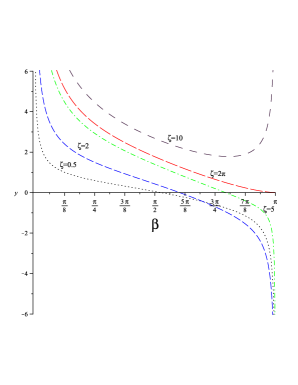
Figure 1: The various curves correspond to values of $\zeta=0.5,2,5,2\pi,10$ and are ordered so that on the left part of the figure (say $\beta$ close to $0$) $\zeta$ increases. In other words, the lower curve corresponds to $\zeta=0.5$, whereas the upper curve to $\zeta=10$.

In our case, this yields

$$\left|{\dot{\sigma}}_{k}^{(0)}(t)\right|_{t_{\rm exit}}$$ (24)

$$= {H^{2}\over 2\sqrt{2}k^{3\over 2}}\left|\xi\left({(\rho\delta-\gamma\sigma)\over\xi(\gamma^{2}+\delta^{2})}\right)^{-{3\over 2}}{{\rm d}\over{\rm d}\xi}\left({(\rho\delta-\gamma\sigma)\over\xi(\gamma^{2}+\delta^{2})}\right)\right|_{\xi=2\pi}$$

$$={2\sqrt{2}\pi^{2}H^{2}\over k^{3\over 2}}\left|{\sqrt{\zeta}(\zeta+2\pi\cos\beta)\over\sqrt{\sin\beta}\sqrt{\zeta^{2}+4\pi\cos\beta+4\pi^{2}}}\right|.$$

The last step follows because $\xi(t_{\rm exit})=2\pi$ at Hubble-scale crossing kiefer . Figure $1$ shows a plot of the function whose absolute value is taken here:

$$f(\zeta,\beta):={\sqrt{\zeta}(\zeta+2\pi\cos\beta)\over\sqrt{\sin\beta}\sqrt{\zeta^{2}+4\pi\cos\beta+4\pi^{2}}},$$ (25)

when $\zeta\in(0,10),\;\beta\in(0,\pi)$. This function exhibits no relative minima or maxima, and hence there are no ‘preferred’ values of $\zeta$ and $\beta$ from a mathematical point of view. The result (24) can be used to obtain the power spectrum kiefer ; calcagni

$$\mathcal{P}^{(0)}(k):=\frac{k^{3}}{2\pi^{2}}\left|\delta_{k}(t_{\rm enter})\right|^{2},$$ (26)

where pad

$$\delta_{k}(t_{\rm enter})={4\over 3}{{\dot{\sigma}}_{k}(t)\over{\dot{\phi}}(t)}\Biggr{|}_{t=t_{\rm exit}},$$ (27)

such that we get

$$\mathcal{P}^{(0)}(k)=\frac{64}{9}\pi^{2}\left|f(\zeta,\beta)\right|^{2}\frac{H^{4}}{\big{|}\dot{\phi}(t)\big{|}^{2}}_{\!\!\!\!t_{\mathrm{exit}}}\!\!\!.$$ (28)

IV Quantum gravitational corrections

Proceeding with the expansion (5) to the next order, which contains terms proportional to $m_{\rm P}^{-2}$, we arrive at a quantum-gravity corrected Schrödinger equation of the form kiefer

$${\rm i}{\partial\over\partial t}\psi_{k}^{(1)}={\cal H}_{k}\psi_{k}^{(1)}-{{\rm e}^{3\alpha}\over 2m_{P}^{2}\psi_{k}^{(0)}}\left[{({\cal H}_{k})^{2}\over V}\psi_{k}^{(0)}\right]\psi_{k}^{(1)},$$ (29)

where

$$V := {\rm e}^{6\alpha}H^{2},\qquad W_{k}:=k^{2}{\rm e}^{4\alpha}+m^{2}{\rm e}^{6\alpha},$$ (30)

$${}{\cal H}_{k} := {1\over 2}{\rm e}^{-3\alpha}\left[-{\partial^{2}\over\partial f_{k}^{2}}+W_{k}f_{k}^{2}\right].$$ (31)

As in Ref. kiefer , we make the following Gaussian ansatz for the corrected wave functions $\psi_{k}^{(1)}$:

$$\psi_{k}^{(1)}=\left(N_{k}^{(0)}(t)+m_{\rm P}^{-2}N_{k}^{(1)}(t)\right)$$

$$\;\times{\rm exp}\left[-{1\over 2}\left(\Omega_{k}^{(0)}(t)+m_{\rm P}^{-2}\Omega_{k}^{(1)}(t)\right)f_{k}^{2}(t)\right].$$ (32)

Here, a second term describing a possible violation of unitarity has been neglected in (29). Such a term was found in the general derivation singh and can be interpreted as follows (see also Ref. kief93 ). The general Wheeler–DeWitt equation is of the Klein–Gordon form, not the Schrödinger form. Expanding the conserved Klein–Gordon type current in powers of $m_{\rm P}^{-2}$, one arrives at order $m_{\rm P}^{0}$ at the exact conservation of the Schrödinger current, and at order $m_{\rm P}^{-2}$ at a violation of this conservation by a term that corresponds to the unitarity-violating term neglected in (IV).

One can estimate that in most situations the unitarity-violating term is negligible compared to the correction term in (IV) singh . But one can also adopt the following viewpoint. After an appropriate redefinition of the wave function, unitarity can be achieved at order $m_{\rm P}^{-2}$ bertoni . Such a procedure was also applied in the context of the quantum-mechanical Klein–Gordon equation in an external gravitational field lammer . Independently of which argument is used, we shall no longer consider the unitarity-violating term in the main body of our paper, but we refer the reader to the Appendix for detailed calculations aimed at further clarifying this crucial issue.

Inserting the ansatz (IV) into (29), one arrives at

$${\rm i}{{\rm d}\over{\rm d}t}\log\left(N_{k}^{(0)}+{N_{k}^{(1)}\over m_{P}^{2}}\right)-{{\rm i}\over 2}\left({\dot{\Omega}}_{k}^{(0)}+{{\dot{\Omega}}_{k}^{(1)}\over m_{P}^{2}}\right)f_{k}^{2}$$ (33)

$$= {1\over 2}{\rm e}^{-3\alpha}\biggr{\{}\Omega_{k}^{(0)}+{1\over m_{P}^{2}}\left[\Omega_{k}^{(1)}-{3\over 4V}\left(\Bigr{(}\Omega_{k}^{(0)}\Bigr{)}^{2}-{2\over 3}W_{k}\right)\right]$$

$$+ \left(W_{k}-\left(\Omega_{k}^{(0)}+{\Omega_{k}^{(1)}\over m_{P}^{2}}\right)^{2}-{3\Omega_{k}^{(0)}(W_{k}-(\Omega_{k}^{(0)})^{2})\over 2Vm_{P}^{2}}\right)f_{k}^{2}$$

$$+{\rm O}(f_{k}^{4})\biggr{\}},$$

which can be cast in the form

$$\sum_{l=0}^{2}A_{2l}f_{k}^{2l}=0$$ (34)

with time-dependent coefficients $A_{2l}$. Setting, in particular, the overall coefficient $A_{2}$ of $f_{k}^{2}$ to zero, one finds the first-order nonlinear equation kiefer

$${\dot{\Omega}}_{k}^{(1)}(t)=-2{\rm i}{\rm e}^{-3\alpha}\Omega_{k}^{(0)}(t)$$

$$\!\!\!\times\left(\Omega_{k}^{(1)}(t)-{3\over 4V(t)}\left[\Bigr{(}\Omega_{k}^{(0)}(t)\Bigr{)}^{2}-W_{k}(t)\right]\right).$$ (35)

Eventually, on defining

$$C:=\rho\delta-\gamma\sigma,\quad D:=\rho\gamma+\sigma\delta,$$ (36)

this reads as follows (since ${\rm e}^{-\alpha}=H\xi/k$)

$${{\rm d}\Omega_{k}^{(1)}\over{\rm d}\xi}={2{\rm i}\xi\over(\gamma^{2}+\delta^{2})}(C+{\rm i}D)\times$$

$$\!\!\!\!\!\!\!\!\!\!\left[\Omega_{k}^{(1)}+{3\over 4}\left(\mu^{2}+\xi^{2}-\xi^{4}{(C^{2}-D^{2}+2{\rm i}CD)\over(\gamma^{2}+\delta^{2})^{2}}\right)\right].$$ (37)

In Ref. kiefer , the desired solution $\Omega_{k}^{(1)}$ is taken to vanish at late times. This expresses the idea that quantum gravitational corrections should tend to zero at large times, which is certainly in agreement with observations. In the next section, we shall discuss a subtlety that arises when solving (IV) with this boundary condition.

V Enhancement or suppression of power at large scales?

Taking as in Ref. kiefer the initial state to be the ground state of Minkowski spacetime, one has to make the choice $\zeta=1$ and $\beta={3\over 2}\pi$. For this case, (IV) reads

$${{\rm d}\Omega_{k}^{(1)}\over{\rm d}\xi}={2{\rm i}\xi\over(\xi-{\rm i})}\Omega_{k}^{(1)}+{3\over 2}\xi^{3}{(2\xi-{\rm i})\over(\xi-{\rm i})^{3}}.$$ (38)

The corresponding solution of (IV) is then inserted into the formula that generalizes (23) at the next-to-leading order kiefer ,

$$\left|{\dot{\sigma}}_{k}^{(1)}(t)\right|=\left|{H\xi\over\sqrt{2}}{{\rm d}\over{\rm d}\xi}\left[\left({\rm Re}\Omega_{k}^{(0)}+m_{\rm P}^{-2}{\rm Re}\Omega_{k}^{(1)}(\xi)\right)^{-{1\over 2}}\right]\right|,$$ (39)

from which one gets

$$\left|{\dot{\sigma}}_{k}^{(1)}(t)\right|_{t_{\rm exit}}=|C_{k}|\left|{\dot{\sigma}}_{k}^{(0)}(t)\right|_{t_{\rm exit}}.$$ (40)

Eventually, the square of the coefficients $C_{k}$ yields the corrected power spectrum (see below).

On requiring $\Omega_{k}^{(1)}(\xi=0)=0$, one finds from (38) the following exact solution:

$$\Omega_{k}^{(1)}(\xi)=-{3\over 8}{\rm e}^{2{\rm i}\xi}{[1+{\rm Ei}(1,2){\rm e}^{2}]\over(1+{\rm i}\xi)^{2}}+\Omega_{k}^{(1,{\rm part})}(\xi),$$ (41)

where

$$\Omega_{k}^{(1,{\rm part})}(\xi) = {3\over 8}{[-5+6(1+{\rm i}\xi)+4{\rm Ei}\left(1,2(1+{\rm i}\xi)\right){\rm e}^{2(1+i\xi)}-4\xi^{2}(1+i\xi)]\over(1+{\rm i}\xi)^{2}}\,,$$ (42)

and ${\rm Ei}(a,z)$ denotes the exponential integral defined by

$${\rm Ei}(a,z):=\int_{1}^{\infty}{{\rm e}^{-tz}\over t^{a}}{\rm d}t.$$ (43)

Here, we have to address the special case

$${\rm Ei}(1,z)\equiv\Gamma(0,z)\equiv E_{1}(z),$$ (44)

cf. Ref. abra , Sec. 5.1. From the exact solution (42), one finds for the coefficients $C_{k}$ defined in (40) the result

$$C_{k}\approx\left(1-{54.37\over k^{3}}{H^{2}\over m_{P}^{2}}\right)^{-{3\over 2}}\left(1+{7.98\over k^{3}}{H^{2}\over m_{P}^{2}}\right),$$ (45)

see Figure $2$. They correspond to an enhancement of the power spectrum compared to its value when quantum-gravity effects are neglected,

$$\mathcal{P}^{(1)}(k)=\mathcal{P}^{(0)}(k)\,C_{k}^{2}$$

$$\!\sim\mathcal{P}^{(0)}(k)\left[1+{89.54\over k^{3}}{H^{2}\over m_{P}^{2}}+{1\over k^{6}}{\rm O}\left({H^{4}\over m_{P}^{4}}\right)\right]^{2}.$$ (46)

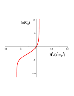
Figure 2: The quantity $\ln(C_{k})$ is plotted as a function of $H^{2}/(k^{3}m_{\rm P}^{2})$ (see Eq. (45)).

In Ref. kiefer , another exact solution of (38) is chosen (although it is there not given in explicit form). The solution has the same form as in (42), but with the exponential integral replaced by the other exponential integral

$${\rm Ei}(z)=-\int_{-z}^{\infty}\frac{{\rm e}^{-t}}{t}{\rm d}t.$$ (47)

¿From this solution, one finds the value $C_{k}$ given in Ref. kiefer ,

$$C_{k}\approx\left(1-{43.56\over k^{3}}{H^{2}\over m_{P}^{2}}\right)^{-{3\over 2}}\left(1-{189.18\over k^{3}}{H^{2}\over m_{P}^{2}}\right).$$ (48)

This solution for $C_{k}$ approaches $1$ at large $k$ (i.e. for small scales), but decreases monotonically to $0$ for small $k$ (i.e. for large scales). In contrast to (45), this solution thus leads to a suppression of power at large scales,

$$\mathcal{P}^{(1)}(k)=\mathcal{P}^{(0)}(k)\,C_{k}^{2}$$

$$\!\!\!\!\!\!\!\!=\mathcal{P}^{(0)}(k)\left[1-{123.83\over k^{3}}{H^{2}\over m_{P}^{2}}+{1\over k^{6}}{\rm O}\left({H^{4}\over m_{P}^{4}}\right)\right]^{2}.$$ (49)

What is the difference between both solution, that is, between the different versions of the exponential integral? Both solutions ${\rm Ei}(z)$ and $E_{1}(z)$ assume the value zero if $\xi=0$. Whereas, however, the solution $E_{1}(z)$ approaches this value continuously (see Figure $3$) , the function ${\rm Ei}(z)$ makes a jump with size $\pi$ in its imaginary part abra , in agreement with the property abra

$$E_{1}(-x\pm{\rm i}0)=-{\rm Ei}(x)\mp{\rm i}\pi,$$

where as above $E_{1}(z):=\int_{z}^{\infty}{{\rm e}^{-t}\over t}{\rm d}t$ when $|{\rm arg}z|<\pi$. Imposing continuity as a reasonable selection criterion for the solution, since our JWKB ansatz for the wave function should be differentiable, would entail the choice of $E_{1}(z)$ and would thus lead to the prediction of an enhancement of power at large scales, unlike the prediction of suppression in Ref. kiefer .

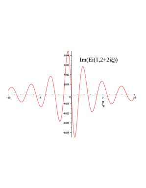
Figure 3: Plot of the imaginary part of ${\rm Ei}(1,2i\xi+2)\equiv E_{1}(2{\rm i}\xi+2$.

Let us now revert to Eq. (38). Remarkably, by passing to the new variable

$$z=1+{\rm i}\xi,$$ (50)

it can be written in the form

$$\frac{{\rm d}\Omega_{k}^{(1)}}{{\rm d}z}=2\left(1-\frac{1}{z}\right)\Omega_{k}^{(1)}+\frac{3}{2}\left(7-2z-\frac{9}{z}+\frac{5}{z^{2}}-\frac{1}{z^{3}}\right),$$ (51)

and the solution reads as

$$\Omega_{k}^{(1)}(z) = P_{1}\frac{{\rm e}^{2z}}{z^{2}}+\frac{3}{8z^{2}}\left[4z^{3}-8z^{2}+10z-5\right.$$ (52)

$$\left.+4{\rm e}^{2z}{\rm Ei}(1,2z)\right]\,,$$

with $P_{1}$ determined so that $\Omega_{k}^{(1)}(1)=0$. The passage to a complex independent variable is therefore very convenient in the course of performing and checking our calculations.

Such a solution can be studied graphically by introducing the complex polar representation for $z=\rho{\rm e}^{{\rm i}\theta}$ and substituting it into the definition of $\Omega_{k}^{(1)}(z)$. On defining the functions

$$f_{\rho}(\theta):={\rm Re}\Bigr{[}\Omega_{k}^{(1)}(\rho{\rm e}^{{\rm i}\theta})\Bigr{]},\;g_{\rho}(\theta):={\rm Im}\Bigr{[}\Omega_{k}^{(1)}(\rho{\rm e}^{{\rm i}\theta})\Bigr{]},$$ (53)

one then finds the behavior displayed in Figures $4$ and $5$.

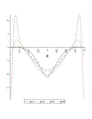
Figure 4: Plots of $f_{1}$, $f_{2}$, $f_{3}$, $f_{4}$ (i.e. fixed values of $\rho=1,2,3,4$) as functions of $\theta$. As $\rho$ increases, the curves show two enhanced peaks at around $\theta=0$ and $\theta=2\pi$.

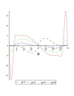
Figure 5: Plots of $g_{1}$, $g_{2}$, $g_{3}$, $g_{4}$ (i.e. fixed values of $\rho=1,2,3,4$) as functions of $\theta$. As $\rho$ increases the curves show two enhanced peaks at around $\theta=0$ and $\theta=2\pi$.

The reader might still be worried by the fact that the limit as $t\rightarrow\infty$ mentioned before and in Ref. kiefer is only of mathematical interest, because it would correspond to eternal inflation, which is physically inconsistent. To answer this question, we begin by noting, from (12), that

$$-{1\over H}{{\rm d}\xi\over\xi}={\rm d}t,$$ (54)

and hence

$$\xi(T)={\rm e}^{-H(T-t_{0})}\xi(t_{0}).$$ (55)

If $T$ denotes the duration of the inflationary stage, it is enough to impose the boundary condition

$$\Omega_{k}^{(1)}(\xi(T))={\widetilde{\varepsilon}},$$ (56)

where, from (55),

$$\xi(T)=\varepsilon\xi(t_{0}).$$ (57)

For example, if $\varepsilon$ is taken to be $10^{-2},10^{-3}...$ and ${\widetilde{\varepsilon}}$ is set to $0$, we still find full agreement with the numerical values in Eq. (45).

If one is instead interested in the deep quantum gravity regime, one has to consider values of $T$ so small that $T-t_{0}<0$ in (55). It is then appropriate to consider the variable

$${\widetilde{\xi}}\equiv{1\over\xi},$$ (58)

in terms of which Eq. (51) becomes

$${{\rm d}\over{\rm d}{\widetilde{\xi}}}\Omega_{k}^{(1)}={2{\rm i}\over{\widetilde{\xi}}^{2}({\rm i}{\widetilde{\xi}}-1)}\Omega_{k}^{(1)}+{3\over 2}{({\rm i}{\widetilde{\xi}}-2)\over{\widetilde{\xi}}^{3}(1-{\rm i}{\widetilde{\xi}})^{3}}.$$ (59)

On defining the complex variable $z\equiv 1+{{\rm i}\over\xi}$, one can then plot $\Omega_{k}^{(1)}$ as a function of such a $z$. To perform a comparison with Figures $4$ and $5$, we plot in Figures $6$ and $7$ the real and imaginary part of the solution of Eq. (59) when the amplitude $\rho$ takes the same values considered in Figures $4$ and $5$. The plots corresponding to $\rho=3,4$ are virtually indistinguishable. The result is not, by itself, enlightening, but it shows that even the deep quantum gravity regime can be further investigated, if necessary.

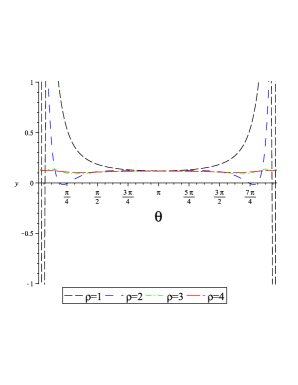
Figure 6: Plot of the real part of the solution of (59) when the amplitude $\rho$ of the complex variable $z=1+{{\rm i}\over\xi}$ equals $1,2,3,4$.

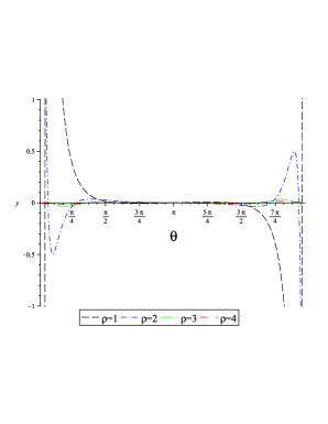
Figure 7: Plot of the imaginary part of the solution of (59) when the amplitude $\rho$ of the complex variable $z=1+{{\rm i}\over\xi}$ equals $1,2,3,4$.

Let us consider finally the general equation (IV). Since the dependence on $\zeta$ and $\beta$ complicates matters, we limit our considerations to its linearization around $\zeta=1$ and $\beta=3/2\pi$ and to the special case $\mu=0$, that is, we look for solutions of the form

$$\Omega_{k}^{(1)}(\xi)={\widetilde{\Omega}}_{k}^{(1)}(\xi)+(\zeta-1)\Omega_{k}^{(1)a}(\xi)+(\beta-3/2\pi)\Omega_{k}^{(1)b}(\xi)\,,$$ (60)

where ${\widetilde{\Omega}}_{k}^{(1)}$ stands for the solution found in kiefer . Substitution of (60) into (IV) gives the following equations:

$$\frac{{\rm d}\Omega_{k}^{(1)a}}{{\rm d}\xi} = -\frac{2{\rm i}\xi}{({\rm i}-\xi)}\Omega_{k}^{(1)a}-\frac{1}{4}\frac{{\rm i}\xi({\rm i}\sin\xi-2\cos\xi-2{\rm i}\cos^{2}\xi\sin\xi+2\cos^{3}\xi)}{({\rm i}\sin\xi-3\cos\xi-4{\rm i}\cos^{2}\xi\sin\xi+\cos^{3}\xi)(i-\xi)^{3}}\cdot{\mathcal{A}}(\xi),$$

$$\frac{{\rm d}\Omega_{k}^{(1)b}}{{\rm d}\xi} = -\frac{2{\rm i}\xi}{({\rm i}-\xi)}\Omega_{k}^{(1)b}+\frac{\xi^{2}(2\cos^{2}\xi-1+2{\rm i}\cos\xi\sin\xi)}{4({\rm i}-\xi)^{4}}\cdot{\mathcal{A}}(\xi)\,,$$ (61)

where

$${\mathcal{A}}(\xi)=12\xi^{4}-6\xi^{2}+18{\rm i}\xi+3+8{\rm e}^{2{\rm i}\xi}P_{1}+12{\rm Ei}(1,2(1+{\rm i}\xi)){\rm e}^{2(1+{\rm i}\xi)},$$ (62)

and $P_{1}=-3/8-3{\rm e}^{2}{\rm Ei}(1,2)/2$. These equations can be studied numerically. Unfortunately, the task turns out to be technically very hard, but these equations are given here because their investigation might shed light on the consequences of choosing another vacuum for the very early universe. This is the subject of future investigations.

VI Observability of the corrections

We have used the uncorrected Schrödinger equation (8) to arrive at expression (24), from which we can immediately obtain the power spectrum (28),

$$\mathcal{P}^{(0)}(k)\propto\frac{H^{4}}{\big{|}\dot{\phi}(t)\big{|}^{2}}_{\!\!\!\!t_{\mathrm{exit}}}.$$ (63)

This corresponds – apart from a dimensionless constant, which is not relevant for the following discussion – to the standard power spectrum of scalar cosmological perturbations calcagni ,

$${\cal P}_{s}^{(0)}(k)={G\over\epsilon\pi}H^{2},$$ (64)

where we have used the first slow-roll parameter defined as

$$\epsilon=-{{\dot{H}}\over H^{2}}=\frac{4\pi G\,\big{|}\dot{\phi}(t)\big{|}^{2}_{t_{\mathrm{exit}}}}{H^{2}}\,.$$ (65)

As we have seen in (V) and (V), the quantum-gravitationally corrected Schrödinger equation leads to a modification of the power spectrum by a correction function $C_{k}$, such that we can translate this modification also to the standard power spectrum in the following way:

$${\cal P}_{s}^{(1)}(k)={\cal P}_{s}^{(0)}(k)\,C_{k}^{2}\,.$$ (66)

Along the lines of calcagni , we write

$$C_{k}^{2}=1+\delta^{\pm}_{\mathrm{WDW}}(k)+{1\over k^{6}}\,{\mathcal{O}}\!\left(\left({H\over m_{\mathrm{P}}}\right)^{4}\right),$$ (67)

where $\delta^{\pm}_{\mathrm{WDW}}(k)$ either takes the form

$$\delta^{+}_{\mathrm{WDW}}(k)={179.09\over k^{3}}\left({H\over m_{\mathrm{P}}}\right)^{2},$$ (68)

which follows from (V), or the form resulting from (V)

$$\delta^{-}_{\mathrm{WDW}}(k)=-\,{247.68\over k^{3}}\left({H\over m_{\mathrm{P}}}\right)^{2}.$$ (69)

The basic equations in the theory of the spectral index $n_{s}$ and its running $\alpha_{s}$ involve the slow-roll parameters calcagni

$$\eta:=-{\ddot{\phi}\over H{\dot{\phi}}}\quad\text{and}\quad\Xi^{2}:={1\over H^{2}}{{\rm d}\over{\rm d}t}{\ddot{\phi}\over{\dot{\phi}}}.$$ (70)

There is thus a change of sign in front of $\delta^{\pm}_{\mathrm{WDW}}$ with respect to the discussion in calcagni , that is,

$$n_{s}-1:={{\rm d}\log{\cal P}_{s}\over{\rm d}\log k}\approx 2\eta-4\epsilon-3\delta^{\pm}_{\mathrm{WDW}}$$ (71)

and

$$\alpha_{s}:={{\rm d}n_{s}\over{\rm d}\log k}\approx 2(5\epsilon\eta-4\epsilon^{2}-\Xi^{2})+9\delta^{\pm}_{\mathrm{WDW}}\,,$$ (72)

where use has been made of the approximate formula calcagni

$${{\rm d}\over{\rm d}\log k}\approx{1\over H}{{\rm d}\over{\rm d}t}\,,$$ (73)

jointly with the equations of motion.

Giving up our definition that $k$ is dimensionless and reinserting a reference wavenumber, which can either correspond to the largest observable scale, $k_{\mathrm{min}}\sim 1.4\times 10^{-4}\,\text{Mpc}^{-1}$ calcagni , or to the pivot scale used in the WMAP9 analysis, $k_{0}=0.002\,\text{Mpc}^{-1}$ calcagni ; Hinshaw12 , we now write $k/k_{\mathrm{min}}$ or $k/k_{0}$, respectively, instead of $k$. Since the ratio $H/m_{\mathrm{P}}$ has to be smaller than about $3.5\times 10^{-6}$ because of the observational bound on the tensor-to-scalar ratio $r<0.11$ for $k_{0}=0.002\,\text{Mpc}^{-1}$ from the Planck 2013 results baumann ; Planck13 , we find that for $k\rightarrow k/k_{0}$ the absolute value of the quantum-gravitational correction is limited by

$$\left|\delta^{+}_{\mathrm{WDW}}(k_{0})\right|\lesssim 2.2\times 10^{-9},\;\;\left|\delta^{-}_{\mathrm{WDW}}(k_{0})\right|\lesssim 3.0\times 10^{-9},$$

while with the replacement $k\rightarrow k/k_{\mathrm{min}}$ this limit is further weakened:

$$\left|\delta^{+}_{\mathrm{WDW}}(k_{0})\right|\lesssim 7.5\times 10^{-13},\;\;\left|\delta^{-}_{\mathrm{WDW}}(k_{0})\right|\lesssim 1.0\times 10^{-12}.$$

The difference for $\delta^{-}_{\mathrm{WDW}}$ compared to calcagni stems from fact that our upper bound for the ratio $H/m_{\mathrm{P}}$ is weaker than the upper bound derived in calcagni from a different assumption. Furthermore, we have used the exact values of (68) and (69) instead of the approximate value $10^{3}$ as in calcagni .

By comparing the quantum-gravitational corrections to the spectral index $n_{s}$ and its running $\alpha_{s}$ derived above with the values determined from the WMAP9 data, $n_{s}=0.9608\pm 0.0080$ and $\alpha_{s}=-0.023\pm 0.011$ (using the WMAP9+eCMB+BAO+$H_{0}$ dataset in both cases) Hinshaw12 , and the 2013 results of the Planck mission, $n_{s}=0.9603\pm 0.0073$ and $\alpha_{s}=-0.013\pm 0.009$ (using additionally the WMAP polarization data in both cases) Planck13 , we see that our corrections are completely drowned out by the statistical uncertainty in the data. Furthermore, one can already rule out that further improvements of the statistics of Planck data and future satellite missions to measure the CMB anisotropies more precisely will push these corrections into observable regions, as the main source for statistical uncertainty on large scales in the anisotropy spectrum is cosmic variance, which is given in terms of spherical multipoles $\ell=2k/k_{\mathrm{min}}$ by (see e.g. knox )

$$\text{Var}_{\mathcal{P}_{s}}(\ell)=\frac{2}{2\ell+1}\,\mathcal{P}^{2}_{s}(\ell)\,.$$ (74)

Defining $\ell_{0}$ as the multipole corresponding to the pivot scale $k_{0}$ given above, $\ell_{0}\approx 29$, the conclusion of the detailed discussion in calcagni , which determines the region in the $\left(\ell,\mathcal{P}_{s}(\ell)/\mathcal{P}_{s}(\ell_{0})\right)$ plane that is affected by cosmic variance can essentially be carried over to the present discussion. The only difference is the sign change for $\delta^{+}_{\mathrm{WDW}}(k)$ and a very slight suppression of the correction if one does not approximate the pre-factors in (68) and (69). The order of magnitude of the correction stays the same and therefore also the conclusion that the quantum-gravitational correction is entirely negligible compared to the error induced by cosmic variance remains.

We can repeat, however, for $\delta^{+}_{\mathrm{WDW}}$ the analysis to determine an upper bound on the energy scale of inflation, which was presented in kiefer for $\delta^{-}_{\mathrm{WDW}}$. Instead of assuming that $C_{k}^{2}$ has to be greater than about $0.95$ in order to be compatible with the observation that the anisotropy spectrum deviates from a scale-invariant spectrum by less than $5\,\%$, we introduce the upper bound that $C_{k}^{2}$ has to be smaller than $1.05$ at $k/k_{0}\sim 1$. From equation (67) and (68), we then immediately obtain the upper bound

$$H\lesssim 1.67\times 10^{-2}\,m_{\mathrm{P}}\approx 4.43\times 10^{17}\,\text{GeV}.$$ (75)

For $\delta^{-}_{\mathrm{WDW}}$ the upper bound is kiefer

$$H\lesssim 1.42\times 10^{-2}\,m_{\mathrm{P}}\approx 3.76\times 10^{17}\,\text{GeV}.$$ (76)

Both constraints are clearly weaker than the already existing observational limits of about $H\lesssim 10^{15}\,\text{GeV}$, but it reassures that the present approach is consistent with these limits.

As a final remark we want to add that the general discussion in calcagni on non-Gaussianities in the squeezed limit arising from quantum-gravitational corrections is not affected by our results in the present paper, and we therefore have to conclude that, at the present state, one cannot expect to see any effect from Wheeler–DeWitt quantum cosmology in the bispectrum.

VII Concluding remarks

We have studied the quantum gravitational corrections terms to the CMB anisotropy spectrum as they are found from a Born–Oppenheimer type of approximation from the Wheeler–DeWitt equation. We have, in particular, discussed a subtlety concerning the central equation (38). Imposing the boundary condition $\Omega_{k}^{(1)}\to 0$ for $\xi\to 0$ (corresponding to the absence of quantum-gravity effects at late times), we have found that there exist two solutions. One of them, which is related to the exponential integral $E_{1}(z)$, is continuous in this limit, whereas the other one, which is related to the exponential integral ${\rm Ei}(z)$ makes a jump in the imaginary part of size $\pi$. Both solutions are in accordance with the requirement that quantum-gravity effects are unobservable at late times. The numerical corrections to the CMB spectrum are of the same order in both cases. There is, however, a qualitative difference. Whereas the continuous solutions leads to an enhancement of power at large scales, the discontinuous solution leads to a suppression. If we adopt continuity as a condition for the allowed solutions, bearing in mind that the JWKB ansatz for the wave function should be differentiable, we have to predict an enhancement of power, unlike kiefer where a suppression is predicted.

So far, these corrections to the CMB power spectrum are too small to be observed. Nevertheless, their size is much bigger than corresponding corrections in laboratory situations. One can thus express the hope that it might eventually be possible to test them in a cosmological setting.

At a field-theoretic level, an interesting issue is whether the various choices of amplitude $\zeta$ and phase $\beta$ in Sec. III and V can describe physically relevant choices of vacuum other than the Bunch–Davies vacuum. A further issue seems to be whether our quantum cosmological calculations can be used to test the recent theoretical prediction of circles in the CMB penrose . These are subjects for future work.

For a full-fledged investigation, one has to repeat our whole analysis by using the gauge-invariant formalism of cosmological perturbation theory mukhanov ; langlois . While this will be postponed to a later paper, we emphasize that the main qualitative features and open problems are clearly seen already in the more restricted analysis presented here.

Modifications of the power spectrum at large scales can also emerge from other situations. Inflationary models with $\Omega_{\rm m}\neq 1$ lead to an enhancement of power for low multipoles Starobinsky , both for open and closed models. A suppression of power is predicted from the consideration of a self-interacting scalar field KS10 , a model of just-enough inflation RS12 , or the introduction of non-commutative geometry TMB03 . Yet other work laura has studied the nonlocal entanglement of the Hubble volume with modes and domains beyond the horizon, finding that this induces a dipole and quadrupole contribution in the CMB. The great challenge is, of course, to distinguish these contributions in possible observations.

Appendix A The unitarity violation issue

We are here going to see how the unitarity issue is solved with an alternative approach that enables us to explicitly verify that no unitarity violations occur. For this purpose, relying upon Ref. bertoni , we start from the equation (see also Sec. 5.4.1 in oup )

$$\hat{H}\Psi(a,\phi)=\left(\frac{\hbar^{2}}{2m_{\rm P}^{2}}\frac{\partial^{2}}{\partial a^{2}}+m_{\rm P}^{2}V(a)+\hat{H}_{M}\right)\Psi(a,\phi)=0,$$ (77)

where $\hat{H}_{M}$ denotes a Hamiltonian depending generically on matter fields $\phi$ whose mass is light, $m_{\phi}\ll m_{\rm P}$. By virtue of this inequality, introducing the Born–Oppenheimer (hereafter BO) approximation

$$\Psi(a,\phi)=\psi(a)\chi(a,\phi),$$ (78)

we obtain

$$\frac{1}{2m_{\rm P}^{2}}\left(\psi\frac{\partial^{2}}{\partial a^{2}}\chi+2\frac{\partial\psi}{\partial a}\frac{\partial\chi}{\partial a}+\chi\frac{\partial^{2}}{\partial a^{2}}\psi\right)+\psi V_{G}\chi+\psi\hat{H}_{M}\chi=0,$$ (79)

with $V_{G}=m_{\rm P}^{2}V(a)$. In our BO approximation or, in other terms, adiabatic approximation, we can neglect the term $\frac{\partial^{2}}{\partial a^{2}}\chi$ because it varies slowly with respect to the scale factor $a$. Hereafter, in order to agree with the notation of Brout , we will use the Dirac-like notation so that $\chi(a,\phi)=\langle a,\phi|\chi\rangle$. Thus, evaluation of $\langle\chi|$ on the equation obtained from (79) upon replacing $\chi(a,\phi)$ with $\langle a,\phi|\chi\rangle$ yields

$$\frac{1}{2m_{\rm P}^{2}}\frac{\partial^{2}}{\partial a^{2}}\psi+V_{G}\psi+\langle\hat{H}_{M}\rangle\psi+\frac{1}{m_{\rm P}^{2}}\left\langle\chi\left|\frac{\partial}{\partial a}\right|\chi\right\rangle\frac{\partial\psi}{\partial a}=0,$$ (80)

where we have assumed $\left\langle\chi|\chi\right\rangle=\int\mbox{d}\phi\chi^{*}\chi=1$. Now we obtain $V_{G}\psi$ from the latter, and substituting it into (79) gives

$$\left[\hat{H}_{M}-\langle H_{M}\rangle\right]|\chi\rangle + \frac{1}{m_{\rm P}^{2}}\frac{\partial\ln\psi}{\partial a}\left[\left.\left|\frac{\partial}{\partial a}\right|\chi\right\rangle\right.$$ (81)

$$- \left.\left\langle\chi\left|\frac{\partial}{\partial a}\right|\chi\right\rangle|\chi\rangle\right]=0.$$

We can obtain the same result by keeping all terms and doing the approximation after the calculation. In fact, from (79), if we evaluate $\langle\chi|$ on the left-hand side and add and subtract $\psi\times(\left\langle\chi|\frac{\partial}{\partial a}|\chi\right\rangle)^{2}$, we get

$$\left[\frac{\hbar^{2}}{2m_{\rm P}^{2}}D^{2}+V_{G}+\langle\hat{H}_{M}\rangle\right]\psi=-\frac{\hbar^{2}}{2m_{\rm P}^{2}}\langle\bar{D^{2}}\rangle\psi,$$ (82)

where we have introduced the operators

$$D:=\frac{\partial}{\partial a}+{\rm i}A,\qquad\bar{D}:=\frac{\partial}{\partial a}-{\rm i}A,$$ (83)

$$A:=-{\rm i}\left\langle\chi\left|\frac{\partial}{\partial a}\right|\chi\right\rangle.$$ (84)

Following BV , the condition $\left\langle\chi|\frac{\partial}{\partial a}|\chi\right\rangle=0$ can be seen as a ‘gauge’ choice and it implies no restriction by virtue of the ‘gauge invariance’ of the full wave function. We choose $\left\langle\chi|\frac{\partial}{\partial a}|\chi\right\rangle=0$ as Eq. (80) suggests because the equation we require for the semiclassical theory of gravity is that in which classical gravity is driven by the mean energy of matter.
Evaluation of $\langle\chi|$ on Eq. (82) and insertion into Eq. (77) leads to

$$\psi(\hat{H}_{M}-\langle\hat{H}_{M}\rangle)\chi+\frac{\hbar^{2}}{m_{\rm P}^{2}}D\psi\bar{D}\chi=-\frac{\hbar^{2}}{2m_{\rm P}^{2}}\psi(\bar{D}^{2}-\langle\bar{D}^{2}\rangle)\chi.$$ (85)

This equation becomes equal to (81) if we define the new wave functions

$$\tilde{\psi} := \exp\left[{\rm i}\int^{a}A\mbox{d}a^{\prime}\right]\psi,$$ (86)

$$\tilde{\chi} := \exp\left[-{\rm i}\int^{a}A\mbox{d}a^{\prime}\right]\chi,$$ (87)

$$\tilde{\Psi} := \tilde{\psi}\tilde{\chi}=\Psi.$$ (88)

At this stage, the BO approximation is imposed by neglecting the terms $\langle\bar{D}^{2}\rangle$ and $\langle\bar{D}^{2}-\langle\bar{D}^{2}\rangle\rangle$ that are related to fluctuations.
The next step is to require that $\psi$ should be the JWKB solution of Eq. (80)

$$\psi=\frac{1}{N}\exp\left[\frac{{\rm i}S}{\hbar}\right],$$ (89)

where $S$ is the classical action defined by the trajectories that solve Eq. (80), and

$$N=\sqrt{\left|\frac{\partial S}{\partial a}\right|}=\sqrt{m_{\rm P}^{2}\dot{a}},$$ (90)

as one can obtain from the JWKB method. Now, substituting this relation in (81), we obtain an equation for $|\chi\rangle$

$$\left[\hat{H}_{M}-\langle H_{M}\rangle\right]|\tilde{\chi}\rangle-\frac{{\rm i}}{m_{\rm P}^{2}}\frac{\partial S}{\partial a}\frac{\partial}{\partial a}|\tilde{\chi}\rangle=0.$$ (91)

The latter might be regarded as a Schrödinger equation for the matter wave function

$$\left(H_{M}-{\rm i}\hbar\frac{\partial}{\partial\eta}\right)|\chi_{s}\rangle=0,$$ (92)

where we have introduced the time derivative through

$${\rm i}\hbar\frac{\partial}{\partial\eta}:=-{\rm i}\frac{\hbar}{m_{\rm P}^{2}}\frac{\partial S}{\partial a}\frac{\partial}{\partial a},$$ (93)

and we have defined the new wave function

$$|\tilde{\chi}_{s}\rangle:=\exp\left[-\frac{{\rm i}}{\hbar}\int^{\eta}\langle\hat{H}_{M}\rangle\mbox{d}\eta^{\prime}\right]|\tilde{\chi}\rangle.$$ (94)

So we note that at the zeroth stage of the JWKB approximation one obtains the usual evolution equation for matter (Schrödinger equation or, in the field-theoretic case, Tomonaga–Schwinger equation) oup .

One may now search for a possible violation of unitary evolution for this matter wave function. In order to check this, we perform all the approximations after the calculation. On considering all terms, (81) becomes

$$\left(H_{M}-{\rm i}\hbar\frac{\partial}{\partial\eta}\right)|\tilde{\chi}_{s}\rangle=$$

$$-\frac{\hbar^{2}}{m_{\rm P}^{2}}\left[-\frac{\partial\log N}{\partial a}\bar{D}+\frac{1}{2}(\bar{D}^{2}-\langle\bar{D}^{2}\rangle)\right]|\tilde{\chi}_{s}\rangle.$$ (95)

Now we can investigate a possible violation of unitarity from the relation

$${\rm i}\frac{\partial}{\partial\eta}\langle\tilde{\chi}_{s}|\tilde{\chi}_{s}\rangle={\rm i}\int\mbox{d}\phi\left[\langle\tilde{\chi}_{s}|\frac{\partial}{\partial\eta}\tilde{\chi}_{s}\rangle-C.C.\right]$$ (96)

$$= \int\mbox{d}\phi\left[\langle\chi|\left(\hat{H}_{M}-\frac{\hbar^{2}}{m_{\rm P}^{2}}\frac{\partial\log N}{\partial a}\bar{D}\right.\right.$$

$$+ \left.\left.\frac{\hbar^{2}}{2m_{\rm P}^{2}}(\bar{D}^{2}-\langle\bar{D}^{2}\rangle\right)|\chi\rangle-C.C.\right]=0,$$

because we have to neglect $\langle\bar{D}^{2}\rangle$ and $\langle\bar{D}^{2}-\langle\bar{D}^{2}\rangle\rangle$ in the BO approximation. Thus, unless one considers a nonHermitian Hamiltonian operator, there is no violation of unitarity.

Now we want to find a relation between our approach and this one. It is indeed possible to rewrite the BO approximation in the form

$$\Psi=\exp\left[\frac{{\rm i}S}{\hbar}\right],$$ (97)

and expanding S in powers of $m_{\rm P}^{2}$

$$S = m_{\rm P}^{2}S_{0}+S_{1}+\frac{1}{m_{\rm P}^{2}}S_{2}+\mathcal{O}\left(\frac{1}{m_{\rm P}^{4}}\right)$$

$$= \left[m_{\rm P}^{2}S_{0}(a)+\frac{1}{m_{\rm P}^{2}}\sigma_{2}(a)\right]\left[S_{1}(a,\phi)+\frac{1}{m_{\rm P}^{2}}\eta_{2}(a,\phi)\right],$$

where we have decomposed $S_{2}(a,\phi)=\sigma_{2}(a)+\eta_{2}(a,\phi)$. Thus, the wave functional becomes

$$\Psi \approx \left(\frac{1}{N_{K}(a)}\exp\left[\frac{{\rm i}m_{\rm P}^{2}}{\hbar}S_{0}+\frac{{\rm i}}{\hbar m_{\rm P}^{2}}\sigma_{2}\right]\right)$$ (99)

$$\left(N_{K}(a)\exp\left[\frac{{\rm i}S_{1}}{\hbar}+\frac{{\rm i}\eta_{2}}{\hbar m_{\rm P}^{2}}\right]\right)$$

$$= \tilde{\psi}_{K}\tilde{\chi}_{K}.$$

In order to obtain the desired equations, we have to substitute these expressions for $\tilde{\psi}_{K}$ and $\tilde{\chi}_{K}$ in (82) and (85). From (82) we have three equations proportional to $\mathcal{O}(m_{\rm P}^{2})$, $\mathcal{O}(m_{\rm P}^{0})$, $\mathcal{O}(m_{\rm P}^{-2})$, respectively,

$$-\frac{1}{2}{S_{0}^{\prime}}^{2}+V=0,$$ (100)

$${\langle\hat{H}_{M}\rangle}_{0}-{\rm i}\hbar\frac{N_{K}^{\prime}S_{0}^{\prime}}{N_{K}}+{\rm i}\hbar\frac{S_{0}^{\prime\prime}}{2}=0,$$

$$\frac{\hbar^{2}}{2}\left(2\frac{{N_{K}^{\prime}}^{2}}{N_{K}^{2}}-2\frac{S_{0}^{\prime}\sigma_{2}^{\prime}}{\hbar^{2}}-\frac{N_{K}^{\prime\prime}}{N_{K}}\right)$$

$$+ {\langle\hat{H}_{M}\rangle}_{-2}=-\frac{\hbar^{2}}{2}{\langle\bar{D}^{2}\rangle}_{0},$$ (102)

where a prime denotes a derivative with respect to $a$. Analogously, from (85) one obtains

$$H_{M}^{0}-\langle\hat{H}_{M}\rangle_{0}+\hbar{\rm i}S_{0}^{\prime}\left(\frac{N_{K}^{\prime}}{N_{K}}+\frac{{\rm i}S_{1}^{\prime}}{\hbar}\right)=0,$$ (103)

$$H_{M}^{-2}-\langle\hat{H}_{M}\rangle_{-2}-\hbar^{2}\frac{N_{K}^{\prime}}{N_{K}}\left(\frac{N_{K}^{\prime}}{N_{K}}+\frac{{\rm i}S_{1}^{\prime}}{\hbar}\right)$$

$$-S_{0}^{\prime}\eta_{2}^{\prime}=\frac{\hbar}{2}\left(\langle\bar{D}^{2}\rangle_{0}-\frac{N_{K}^{\prime\prime}}{N_{K}}-{\rm i}\frac{S_{1}^{\prime\prime}}{\hbar}+\frac{{S_{1}^{\prime\prime}}^{2}}{\hbar}-2\frac{{\rm i}S_{1}^{\prime}}{\hbar}\frac{N_{K}^{\prime}}{N_{K}}\right),$$

to $\mathcal{O}(m_{\rm P}^{0})$ and $\mathcal{O}(m_{\rm P}^{-2})$ respectively (where we have defined the $c$-number $H_{M}$ by $\hat{H}_{M}|\tilde{\chi}_{K}\rangle=H_{M}|\tilde{\chi}_{K}\rangle$). By comparing terms $\mathcal{O}(m_{\rm P}^{0})$, $\mathcal{O}(m_{\rm P}^{-2})$ we have

$$H_{M}^{0}+\frac{{\rm i}\hbar S_{0}^{\prime\prime}}{2}-S_{0}^{\prime}S_{1}^{\prime}=0,$$ (105)

$$-S_{0}^{\prime}\eta_{2}^{\prime}+H_{M}^{-2}-S_{0}^{\prime}\sigma_{2}^{\prime}+{\rm i}\hbar\frac{S_{1}^{\prime\prime}}{2}-\frac{{S_{1}^{\prime}}^{2}}{2}=0,$$ (106)

respectively, where we have expanded $H_{M}=H^{2}_{M}+H^{0}_{M}+H^{-2}_{M}+\ldots$. As one can see, (8) and (29) are identical to (105) and (106) if we choose $H_{M}=H_{k}$. To perform the calculation of the possible violation of unitarity, it is extremely useful to note that the condition $\langle\chi|\bar{D}|\chi\rangle=0$ becomes

$$\langle\chi|\bar{D}|\chi\rangle = \langle\tilde{\chi}|\frac{\partial}{\partial a}|\tilde{\chi}\rangle=0,$$

$$\langle\tilde{\chi}_{Ks}|\frac{\partial}{\partial a}|\tilde{\chi}_{Ks}\rangle = \int\mbox{d}\phi\left[\tilde{\chi}^{*}_{K}\left(\frac{N_{K}^{\prime}}{N_{K}}+{\rm i}\frac{S_{1}^{\prime}}{\hbar}+{\rm i}\frac{\eta_{2}^{\prime}}{m_{\rm P}^{2}\hbar}\right)\tilde{\chi}_{K}\right]$$ (107)

$$= 0.$$

In the same way, as in (A), for the $\mathcal{O}(m_{\rm P}^{-2})$ we obtain

$$\left[\left(H_{M}^{0}+\frac{1}{m_{\rm P}^{2}}H_{M}^{-2}\right)-{\rm i}\frac{\partial}{\partial\eta}\right]|\tilde{\chi}_{Ks}\rangle$$

$$= \left[\frac{\hbar^{2}}{m_{\rm P}^{2}}\left(\frac{{N_{K}^{\prime}}^{2}}{N_{K}^{2}}+{\rm i}\frac{N_{K}^{\prime}S_{1}^{\prime}}{\hbar}\right)\right.$$

$$+ \frac{\hbar^{2}}{2m_{\rm P}^{2}}\biggr{(}\left\langle\tilde{\chi}\left|\left(\frac{\partial^{2}}{\partial a^{2}}\right)\right|\tilde{\chi}\right\rangle_{0}$$

$$- \left.\frac{N_{K}^{\prime\prime}}{N_{K}}-{\rm i}\frac{S_{1}^{\prime\prime}}{\hbar}+\frac{{S_{1}^{\prime}}^{2}}{\hbar^{2}}-2{\rm i}\frac{N_{K}^{\prime}S_{1}^{\prime}}{\hbar N_{K}}\right)\biggr{]}|\tilde{\chi}_{Ks}\rangle.$$

Performing the same calculation as in (96), we finally obtain the same result

$${\rm i}\hbar\frac{\partial}{\partial\eta}\langle\tilde{\chi}_{Ks}|\tilde{\chi}_{Ks}\rangle$$ (109)

$$= -\frac{{\rm i}S_{0}^{\prime}}{m_{\rm P}^{2}}\int\mbox{d}\phi\left[\tilde{\chi}_{K}\frac{\partial}{\partial a}\tilde{\chi}_{K}+C.C.\right]=0.$$

To summarize, an appropriate redefinition of the wave functions leads to a description without unitarity violation. This is why we can safely neglect the corresponding term in the corrected Schrödinger equation (29). It is, however, an open issue which of the wave functions (the original or the redefined one) is the relevant one in the sense of a quantum measurement process.

References

- (1) G. Gamow, Phys. Rev. 70, 572 (1946).
- (2) A. A. Penzias and R. W. Wilson, Ap. J. 142, 419 (1965).
- (3) G. F. Smoot et al., Ap. J. Lett. 396, L1 (1992).
- (4) D. N. Spergel et al., Ap. J. Suppl. Ser. 148, 175 (2003).
- (5) E. Komatsu et. al., Ap. J. Suppl. Ser. 192, 18 (2011).
- (6) S. W. Hawking, Commun. Math. Phys. 43, 199 (1975).
- (7) C. Kiefer, Quantum Gravity, International Series of Monographs on Physics 155, third edition (Oxford University Press, Oxford, 2012).
- (8) G. Esposito, arXiv:1108.3269v1 [hep-th].
- (9) G. Amelino-Camelia, C. Lämmerzahl, A. Macias, and H. Müller, AIP Conf. Proc. 758, 30 (2005).
- (10) C. Kiefer and T. P. Singh, Phys. Rev. D 44, 1067 (1991).
- (11) A. O. Barvinsky and C. Kiefer, Nucl. Phys. B 526, 509 (1998).
- (12) C. Kiefer, T. Lück, and P. Moniz, Phys. Rev. D 72, 045006 (2005).
- (13) C. Kiefer and M. Krämer, Phys. Rev. Lett. 108, 021301 (2012).
- (14) C. Kiefer and M. Krämer, Int. J. Mod. Phys. D 21, 1241001 (2012).
- (15) G. Calcagni, arXiv:1209.0473v1 [gr-qc].
- (16) M. Bojowald, G. Calcagni, and S. Tsujikawa, Phys. Rev. Lett. 107, 211302 (2011).
- (17) I. Agullo, A. Ashtekar, and W. Nelson, arXiv:1302.0254v1 [gr-qc].
- (18) J. J. Halliwell and S. W. Hawking, Phys. Rev. D 31, 1777 (1985).
- (19) L. Parker and D. Toms, Quantum Field Theory in Curved Space–time (Cambridge University Press, Cambridge, 2009).
- (20) D. Schuch, SIGMA 4, 043 (2008).
- (21) J. Guven, B. Lieberman, and C. T. Hill, Phys. Rev. D 39, 438 (1989).
- (22) N. Bartolo, E. Komatsu, S. Matarrese, and A. Riotto, Phys. Rep. 402, 103 (2004).
- (23) P. Peter and J.-P. Uzan, Primordial Cosmology (Oxford University Press, Oxford, 2009).
- (24) T. S. Bunch and P. C. W. Davies, Proc. R. Soc. Lond. A 360, 117 (1978).
- (25) T. Padmanabhan, Structure Formation in the Universe (Cambridge University Press, Cambridge, 1993).
- (26) C. Kiefer, in: Canonical Gravity: From Classical to Quantum, edited by J. Ehlers and H. Friedrich (Springer, Berlin, 1994); see gr-qc/9312015v1 for a related version.
- (27) C. Bertoni, F. Finelli, and G. Venturi, Class. Quantum Grav. 13, 2375 (1996).
- (28) C. Lämmerzahl, Phys. Lett. A 203, 12 (1995).
- (29) M. Abramowitz and I. A. Stegun, Handbook of Mathematical Functions (Dover, New York, 1964).
- (30) G. Hinshaw et al., arXiv:1212.5226v2 [astro-ph.CO].
- (31) D. Baumann et al., AIP Conf. Proc. 1141, 10 (2009).
- (32) Planck Collaboration, arXiv:1303.5076v1 [astro-ph.CO].
- (33) L. Knox and M. S. Turner, Phys. Rev. Lett 73, 3347 (1994).
- (34) V. G. Gurzadyan and R. Penrose, arXiv:1104.5675v1 [astro-ph.CO].
- (35) V. F. Mukhanov, H. A. Feldman, and R. H. Brandenberger, Phys. Rep. 215, 203 (1992).
- (36) D. Langlois, Class. Quantum Grav. 11, 389 (1994).
- (37) A. A. Starobinsky, in: Cosmoparticle Physics 1, edited by M. Yu. Khlopov and M. E. Prokhorov (Editions Frontières, Gif-sur-Yvette, 1996); see astro-ph/9603075v1 for a related version.
- (38) F. Kühnel and D. J. Schwarz, Phys. Rev. Lett. 105, 211302 (2010).
- (39) E. Ramirez and D. J. Schwarz, Phys. Rev. D 85, 103516 (2012).
- (40) S. Tsujikawa, R. Maartens, and R. Brandenberger, Phys. Lett. B 574, 141 (2003).
- (41) L. Mersini-Houghton and R. Holman, J. Cosmol. Astropart. Phys. 02 (2009) 006.
- (42) R. Brout, Found. Phys. 17, 603 (1987).
- (43) R. Brout and G. Venturi, Phys. Rev. D 39, 2436 (1989).