Active Control of the Parametric Resonance in the Modified Rayleigh-Duffing Oscillator

Abstract

The present paper examines the active control of parametric resonance in modified Rayleigh-Duffing oscillator. We used the method of averaging to obtain steady-state solutions. We have found the critical value of the parametrical amplitude which indicates the boundary layer where the control is efficient in reducing the amplitude vibration. We have also found the effects of excitation parameters and time-delay on dynamical of this system with the principal parametric resonance. We have obtained for this oscillator the Hopf bifurcation and saddle-node bifurcation for certains values of parametric parameters and time-delay. We have studied the influence of parameter $k_{2}$ which is one of the parameters which modify the ordinary Rayleigh-Duffing oscillator. We have discussed the appropriate choice of the time-delay and control gain. We finally studied the stability of fixed point and it is found that the appropriate choice of the time-delay can broaden the stable region of the non-trivial steady-state solutions which will enhance the control efficiency. Numerical simulations are performed in order to confirm analytical results.

Institut de Mathématiques et de Sciences Physiques, BP: 613 Porto Novo, Bénin

keywords: Active control, parametric resonance, modified Rayleigh-Duffing oscillator, stability, bifurcations.

1 Introduction

In recent years, a twofold interest has attracted theoretical, numerical, and experimental investigations to understand the behavior of nonlinear oscillators. Theoretical (fundamental) investigations reveal their rich and complex behavior, and the experimental (self-excited oscillators) describes the evolution of many biological, chemical, physical, mechanical, and industrial systems [1, 2, 3]. Recently, the chaotic behavior of these oscillators is exploited in the field of communication for coding information [4]. The considerable efforts have been devoted to the control of vibrating structures in various fields of fundamental and applied sciences. Two major aims in the scope of the researchers are: reduce the amplitude of vibrations, inhibit chaos and escape from potential well. Applications are well encountered in structural mechanics (see Refs. [1–5]). Parametric excitation occurs in a wide variety of engineering application (Refs. [10-14]). Among various types of control strategies, the active feedback control usually developed by means of electromagnetic force or by a mechanical device ( Ref.[5–9]) and the parametric. In [15] Xin-Ye and al demonstrated that in the dynamical behaviour of a parametrically excited Duffing–Van der Pol oscillator under linear-plus-nonlinear state feedback control with a time-delay, nontrivial steady state responses may lose their stability by a saddle-node bifurcation or Hopf bifurcation as parameters vary. M.Siewe Siewe and al [16] studied the dynamics of a parametrically excited Rayleigh–Duffing oscillator state feedback control with a time-delay, nontrivial steady state solutions may lose their stability by a saddle-node bifurcation or Hopf bifurcation as parameters vary.

Our objective in this paper is to control the amplitude vibration of a parametrically excited modified Rayleigh-Duffing oscillator with time-delayed feedback position and linear velocity terms. The modified Rayleigh-Duffing oscillator that we consider in this work is governed by following equation:

$$\ddot{x}+\epsilon\alpha\dot{x}+\epsilon\beta\dot{x}^{2}+\epsilon\gamma\dot{x}^{3}-2\epsilon k_{1}\dot{x}x+\epsilon k_{2}\dot{x}^{2}x+(\delta+\epsilon a\cos 2\omega_{0}t)x$$ (1)

$$+\epsilon\lambda x^{3}=0.$$ (2)

We used the method of averaging to study this oscillator. The amplitude peak of the parametric resonance can be reduced by means of a correct choice of the time-delay and the feedback gain. We discussed how the existence region of steady-state solutions is modified by the feedback control and we showed the existence regions of the nontrivial solution in the plane of the parametric excitation amplitude and the detuning parameter for an uncontrolled system, a controlled system without time-delay, and those with time-delays corresponding to the minimum and maximum values of an appropriate equivalent damping. A bifurcation analysis and parametric excitation-response and frequency-response curves are presented. We found the effect of the parameter $k_{2}$ on the control. Then we performed a stability analysis of the bifurcation of the model and we derived sufficient conditions for stable non trivial solutions in order to exclude the presence of modulated motion.

2 Model and linear control

2.1 Model

Consider the modified Rayleigh-Duffing oscillator equation which describes the glycolytic reaction catalized by phosphofructokinase, namely the Selkov equations and abstract trimolecular chemical reaction namely Brusselator equation[17].

$$\frac{d^{2}\xi}{dt^{2}}+\tilde{\lambda}\frac{d\xi}{dt}+\tilde{\lambda}^{\prime\prime}(\frac{d\xi}{dt})^{2}+\tilde{\lambda}^{\prime}(\frac{d\xi}{dt})^{3}+\Omega^{2}(1-k\frac{d\xi}{dt})^{2}\xi=0$$ (3)

Perturbing this system by Duffing force and parametric excitation force, we obtained the parametric dissipative modified Rayleigh-Duffing oscillator which is expressed by Eq. (2). We noticed that this equation present another applications. For example, first, it is a model of the El Ni$\tilde{n}$o Southern Oscillation (ENSO) coupled tropical ocean-atmosphere weather phenomenon ([23], [24]) in which the state variables are temperature and depth of a region of the ocean called the thermocline. The annual seasonal cycle is the parametric excitation. The model exhibits a Hopf bifurcation in the absence of parametric excitation. The second application involves a MEMS device ([25], [26]) consisting of a $30\mu m$ diameter silicon disk which can be made to vibrate by heating it with a laser beam resulting in a Hopf bifurcation. The parametric excitation is provided by making the laser beam intensity vary periodically in time.

We consider a single-degree-of-freedom model with a nonlinear soft spring, a linear damper and a linear displacement feedback control system. The model is described by the following differential equation system:

$$\ddot{x}+\epsilon\alpha\dot{x}+\epsilon\beta\dot{x}^{2}+\epsilon\gamma\dot{x}^{3}-2\epsilon k_{1}\dot{x}x+\epsilon k_{2}\dot{x}^{2}x+(\delta+\epsilon a\cos 2\omega_{0}t)x$$ (4)

$$+\epsilon\lambda x^{3}-\epsilon bx(t-\tau)-\epsilon c\dot{x}(t-\tau)=0,$$ (5)

where $x$,$\dot{x}$, $\ddot{x}$ are displacement, velocity and acceleration respectively; $\omega_{0}$ is the natural frequency, $\epsilon$ is a positive parameter, $\alpha,\beta,\gamma,k_{1},k_{2},\delta,\lambda,a$ are constants , $b$ and $c$ are the control gain parameters and $\tau$ is time-delay parameter. In this equation, $-\epsilon bx(t-\tau)-\epsilon c\dot{x}(t-\tau)$ is the feedback force in the system. The resonances appear when $\delta=\omega_{0}^{2}+\epsilon\delta_{1}$.

2.2 Linear control

In this part, we used the method of averaging to study Eq. (5) and to research the controlling domain. In the absence of the parameter $\epsilon$, Eq.(5) reduces to

$$\ddot{x}+\omega_{0}^{2}x=0,$$ (6)

with the solution:

$$x=A\cos(\omega_{0}t+\phi).$$ (7)

If $\epsilon\neq 0$, $A$ and $\phi$ depend on time t. In this condition, differentiating Eq.(7), we find that Eq. (5) is divided into:

$$\frac{dA}{dt} = -\epsilon F[A\cos(\omega_{0}t+\phi),-A\omega_{0}\sin(\omega_{0}t+\phi)]\sin(\omega_{0}t+\phi)$$ (8)

$$A\frac{d\phi}{dt} = -\epsilon F[A\cos(\omega_{0}t+\phi),-A\omega_{0}\sin(\omega_{0}t+\phi)]\cos(\omega_{0}t+\phi),$$ (9)

where

$$F=F(x,\dot{x})=-\alpha\dot{x}-\beta\dot{x}^{2}-\gamma\dot{x}^{3}+2k_{1}\dot{x}x-k_{2}\dot{x}^{2}x$$ (10)

$$-(\delta_{1}+a\cos 2\omega_{0}t)x-\lambda x^{3}+bx(t-\tau)+c\dot{x}(t-\tau).$$ (11)

Using the method of averaging, replacing the right-hand sides of Eq. 9 by their averages over one period of the system with $\epsilon=0$, we obtain

$$\frac{dA}{dt} = -\frac{\epsilon}{T_{0}}\int_{0}^{T_{0}}F[A\cos(\omega_{0}t+\phi),-A\omega_{0}\sin(\omega_{0}t+\phi)]\sin(\omega_{0}t+\phi)dt$$ (12)

$$A\frac{d\phi}{dt}=-\frac{\epsilon}{T_{0}}\int_{0}^{T_{0}}F[A\cos(\omega_{0}t+\phi),-A\omega_{0}\sin(\omega_{0}t+\phi)]\cos(\omega_{0}t+\phi)dt,$$ (13)

where $T_{0}$ is the natural period of this oscillator. Using $x$ and its derivative, Eq.(11) becomes

$$F[A\cos(\omega_{0}t+\phi),-A\sin(\omega_{0}t+\phi)]=\alpha\omega_{0}A\sin(\omega_{0}t+\phi)$$ (14)

$$-\beta\omega_{0}^{2}A^{2}\sin^{2}(\omega_{0}t+\phi)+\gamma\omega_{0}^{3}A^{3}\sin^{3}(\omega_{0}t+\phi)+2k_{1}\omega_{0}A^{2}\sin(\omega_{0}t+\phi)\times$$ (15)

$$\cos(\omega_{0}t+\phi)-k_{2}A^{3}\omega_{0}^{2}\sin^{2}(\omega_{0}t+\phi)\cos(\omega_{0}t+\phi)$$ (16)

$$-(\delta_{1}+a\cos 2\omega_{0}t)A\cos(\omega_{0}t+\phi)-\lambda A^{3}\cos^{3}(\omega_{0}t+\phi)$$ (17)

$$+b\tilde{A}\cos[\omega_{0}(t-\tau)+\tilde{\phi}]-c\omega_{0}\tilde{A}\sin[\omega_{0}(t-\tau)+\tilde{\phi}],$$ (18)

where $\tilde{A}=A(t-\tau)$ and $\tilde{\phi}=\phi(t-\tau)$.

Substituting Eq.(18) into Eq.(12) and Eq.(13) and evaluating the integrals, we find

$$\frac{dA}{dt} = -\frac{\epsilon}{4}[\omega_{0}A(2\alpha+\frac{3}{2}\gamma\omega_{0}^{2}A^{2})-aA\sin 2\phi$$ (20)

$$+2b\tilde{A}\sin(\phi-\tilde{\phi}+\omega_{0}\tau)-2c\omega_{0}\tilde{A}\cos(\phi-\tilde{\phi}+\omega_{0}\tau)],$$

$$A\frac{d\phi}{dt} = \frac{\epsilon}{4}[2\delta_{1}A+\frac{1}{2}(k_{2}+3\lambda)A^{3}\omega_{0}^{2}+aA\cos 2\phi$$ (22)

$$-2b\tilde{A}\cos(\phi-\tilde{\phi}+\omega_{0}\tau)+2c\omega_{0}\tilde{A}\sin(\phi-\tilde{\phi}+\omega_{0}\tau)].$$

Eqs.(20) and (22) show that A and $\phi$ are $O(\epsilon)$. Expanding in Taylor series $\tilde{A},\tilde{\phi}$:

$$\tilde{A} = A(t-\tau)=A(t)-\tau\dot{A}(t)+\tau^{2}\ddot{A}(t)+...,$$ (23)

$$\tilde{\phi} = \phi(t-\tau)=\phi(t)-\tau\dot{\phi}(t)+\tau^{2}\ddot{\phi}(t)+....$$ (24)

Eqs.(23) and (24) indicate that we can replace $\tilde{A}$ and $\tilde{\phi}$ by A and $\phi$ in Eqs.(20) and (22) since $\dot{A},\dot{\phi}$ and $\ddot{A},\ddot{\phi}$ are $O(\epsilon)$ and $O(\epsilon^{2})$ respectively. This reduces an infinite-dimensional problem in functional analysis to a finite-dimensional problem by assuming that the product $\epsilon\tau$ is small [16]. By setting $t=\tilde{t}/\epsilon$ as the new time scale, we have the following averaged equations:

$$\dot{A} = \frac{A}{4}[\omega_{0}(-2\alpha-\frac{3}{2}\gamma\omega_{0}^{2}A^{2})+a\sin 2\phi-2b\sin\omega_{0}\tau$$ (26)

$$+2c\omega_{0}\cos\omega_{0}\tau],$$

$$A\dot{\phi} = \frac{A}{4}[2\delta_{1}+\frac{1}{2}(k_{2}+3\lambda)A^{2}\omega_{0}^{2}+a\cos 2\phi-2b\cos\omega_{0}\tau$$ (28)

$$+2c\omega_{0}\sin\omega_{0}\tau].$$

Seeking steady state, we have $\dot{A}=0$ and $A\dot{\phi}=0$ in Eqs.(26) and (28). A trivial solution is $A=0$ and we find the non trivial solutions verify the equation:

$$A_{0}^{4}-2PA_{0}^{2}+Q=0,$$ (29)

where $\gamma=-\alpha=\mu$ the quantities P and Q are given by

$$P = \frac{4}{9[\mu^{2}\omega_{0}^{6}+(\frac{1}{3}k_{2}\omega_{0}^{2}+\lambda)^{2}]}[3\mu^{2}\omega_{0}^{4}-\delta_{1}(k_{2}\omega_{0}^{2}+\lambda)-$$ (32)

$$(3\mu b\omega_{0}^{2}+(k_{2}\omega_{0}^{2}+3\lambda)c)\omega_{0}\sin\omega_{0}\tau+$$

$$(3\mu b\omega_{0}^{4}+(k_{2}\omega_{0}^{2}+3\lambda)b)\cos\omega_{0}\tau],$$

Indeed P and Q can be rewritten as:

$$Q = \frac{4}{9[\mu^{2}\omega_{0}^{6}+(\frac{1}{3}k_{2}\omega_{0}^{2}+\lambda)^{2}]}[K-8bc\omega_{0}\sin 2\omega_{0}\tau+$$ (34)

$$8(\delta_{1}c\omega_{0}-\mu\omega_{0}b)\sin\omega_{0}\tau+8(-\delta_{1}b+\mu\omega_{0}^{2}c)\cos\omega_{0}\tau],$$

with

$$K=4\omega_{0}^{2}\mu^{2}+4\omega_{0}^{2}c^{2}+4\delta_{1}^{2}+4b^{2}-a^{2}.$$ (35)

Now, solving the equation (29), we obtain

$$A_{0}=\sqrt{P\pm\sqrt{P^{2}-Q}}$$ (36)

For $A_{0}$ real, we require $P>0,Q>0,P^{2}>Q$ or $Q<0$.

We denoted by $A_{0c}$ and $A_{0u}$ the amplitude of the controlled system (i.e. when $b\neq 0$ and $c\neq 0$) and the amplitude of the uncontrolled system respectively [16]. Using these conditions, from Eq.(36), the boundary separating the domain where the control is efficient (reduction in the amplitude of oscillation) to the domain where it is inefficient is given by:

$$a_{c}^{2} = \frac{1}{(P_{c}+P_{u})^{2}}[(4\omega_{0}^{2}\alpha^{2}+4\delta_{1}^{2})(P_{c}+P_{u})^{2}+Q_{1}(P_{c}^{2}+P_{c}P_{u})$$ (38)

$$+\frac{Q_{1}^{2}}{\omega_{0}^{4}[9\gamma^{2}\omega_{0}^{2}+(k_{2}+3\lambda)^{2}]}],$$

where $Q_{1}$ is defined by

$$Q_{1} = 4b^{2}+4\omega_{0}^{2}c-8\omega_{0}bc\sin 2\omega_{0}\tau+8\omega_{0}(c\delta_{1}+\alpha b)\sin\omega_{0}\tau$$ (40)

$$-8(b\delta_{1}+c\alpha\omega_{0}^{2})\cos\omega_{0}\tau,$$

where $P_{c}$ and $P_{u}$ represent the function corresponding to the controlled and uncontrolled system.

To validate our technical control in reducing the amplitude vibration, we have simulated numerically the set of eq.(38). We have plotted in Fig. 1 for two conditions $c>b$ and $b>c$, the domain in the space parameters$(\tau,a_{c})$ where the control is efficient in reducing the amplitude of the oscillations. (a) and (b) represent the case where $k_{2}=0.5$ and (c) corresponds to $k_{2}=12$. We remark that the critical value of amplitude excitation $a$ is lower in the case where the control gain parameters verify the inequality $c>b$. We notice also that the domain where the control is efficient is greater because the peak value of the parameter $a$ is more upper than $k_{2}=0.5$ when $b>c$. For example, when the parameter $k_{2}$ increases or $b$ and $c$ increase, boundary separating the domain where the control is efficient from the domain where the control is inefficient are reversed in a small area ($\tau\in[1.63437,2.45168]$ and $\tau\in[0.524655,0.742604]$ respectively). Fig.2 represents the frequency- and force-response curves resulting from eq.(36) and the results obtained in Fig.1 are clearly verified. We see that the steady-state response of the system is lower when the parameter $a$ is below the boundary domain obtained in Fig.1(b). Now we have plotted in Fig.3 the surface amplitude for two conditions for b, where c is fixed. (a) corresponds to $b=0.3,c=0.5$ while for (b), $b=0.7,c=0.5$. We noticed from Fig.3(a) that the maximum value of the amplitude of steady-state solutions are lower compared to the one obtained in Fig.3(b). This differents simulations prove that our technical is confirmed. From Fig.3, one can see that there are range of time delay $\tau$ and detuning parameters $\delta_{1}$ where the steady-state solution is zero. This can be a consequence of noise effect.

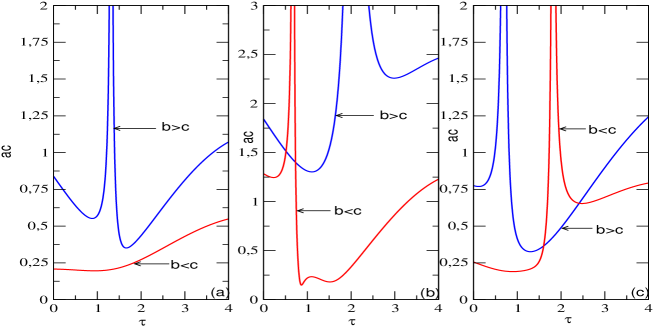
Figure 1: Boundary criterion for the effectiveness of control of the oscillation amplitude in the space$(a_{c},\tau)$ for (a) $k_{2}=0.5$ , (c) $k_{2}=12$; blue curve corresponding to $b=0.35$ and red curve corresponding to $b=0.1$, the other parameters are $\mu=0.002;\lambda=-1;\delta_{1}=0.01;c=0.25$ and (b) $k_{2}=0.5;b=0.5;c=0.3$.

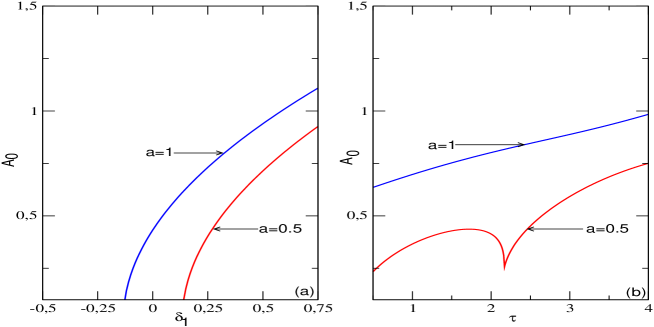
Figure 2: The effect of reducing the steady-state response with control parameter $a$ obtained in Fig.1 (a). (a) Frequency-response and (b) force-response.

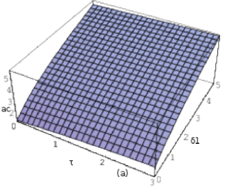
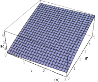
Figure 3: Time-delayed position gain $b$ effect on response-surface curves given by Eq. (22): left curve corresponding to $b=0.3$ and right curve corresponding to $b=0.7$.

3 Effects of the parameters in presence

In this section, we study separately the effects of gain parameters, parametric excitation, and combined gain parameters and parametric excitation in the response from eq.(36) of our model amplitude.

3.1 Effects of parametric excitation alone with null value of $\tau$

The effects of parametric excitation are found from eq.(36) with time delay equal zero. We have plotted in Fig.4, the frequency- and forces-responses of the non trivial solution for $b\neq 0$ and $c\neq 0$. For each values chosen for amplitude or frequency of parametric excitation, we plotted two curves. In Fig.4(a) , we see the limits of curves correspond to stable and unstable for the nontrivial solution. For each value of $a$, the two curves are the same from certains values of $\delta_{1}$. We noticed also that for fixed parametric amplitude, two symetric branches appear around the point near the origin. The reduction effect due to the parameter $a$ is quite important and is found to be visible only in a small region of detuning parameter surrounding this point. Fig.4(b) represents the force-response for two differents values of $\delta_{1}$. It is clear that the Hopf bifurcation with multi-solution occurs as the detuning parameter $\delta_{1}$ increases. We have also found that the saddle-node bifurcation disappears for lower values of $\delta_{1}$.

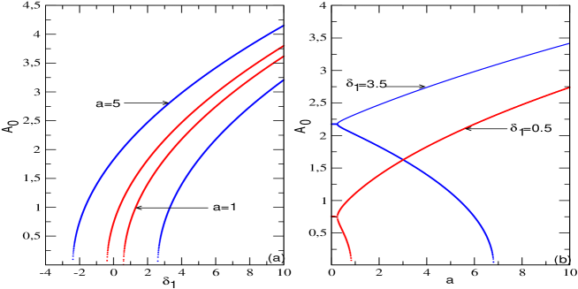
Figure 4: (a) The effect of the parametric amplitude in the frequency-response of the system in the absence of the time-delay. (b) Force-response for two detuning parameter values. Here $b=0.1,\mu=0.002,\lambda=−1,k_{2}=0.5$, and $c=0.5$.

3.2 Effects of control gain parameters for $a$ equal to zero

In this part we have found the control gain parameters effects when the parametric excitation $a$ equal to zero. Fig.5 illustrated the frequency-response of the system for different situations for fixed parameters. (a) and (b) represent for each figure the frequency-response of system respectively for $a=0$, $c=0$ and $a=0$, $c=0$. In Fig.5 $\tau=0.008,\mu=0.8,k_{2}=0.5$ (c) and (d) $\tau=0.008,\mu=0.002,k_{2}=12$. We obtain in each case of this figure that unstable and stable solutions curves are the same. We have also found that the two control gain parameters increases the region of the detuning parameter which is more visible when the time-delayed position is considered alone than the case where the time-delayed velocity is considered alone. Fig.5 (a), (b) compared to Fig.5 (c), (d), prove that the self-excitation parameters $\alpha,\gamma$ and $k_{2}$ affected also the peak of amplitude of vibration which is greater in the case of time-delayed position.

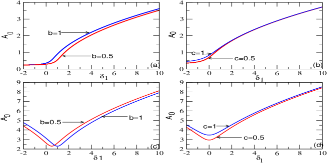
Figure 5: (a) The effect of the position time-delay alone in the frequency-response of the system without parametric excitation and (b) the effect of the velocity time-delay alone in the frequency-response of the system without parametric excitation for $\tau=0.008,\mu=0.8$ and $k_{2}=0.5$.

3.3 Effects of combined parametric excitation and control gain parameters

In this part, we have plotted in space the $(A_{0},\delta_{1})$ and $(A_{0},a)$ corresponding respectively to frequency-response and force-response for non-zero time delay , $\mu=0.8,k_{2}=0.5$. This Fig.6 are used to analysis the effects of combined parametric excitation and control gain parameters. We have developped the similar comments obtained in Fig.4 but the domain of differents bifurcations is not the same. Through Figs. 6 (a), (b), (c) and (d) we conclude that the parameter $k_{2}$ have influenced the system behavior.

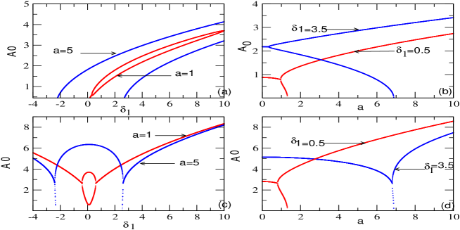
Figure 6: Effect of parametric perturbation added to the time-delayed term in the response of the system. (a) Frequency-response amplitude and (b) $k_{2}=0.5$ Force-response. The values of the parameters are $\tau=0.008,\mu=0.8,b=0.1,\lambda=−1$, $c=0.25$ and $(a),(b)k_{2}=0.5$ and $(c),(d)k_{2}=12$.

4 Stability analysis of solutions

In this case, consider the equilibrium points defined by eq.(36). To study the behavior of the steady state, we resort to the linearized stability principle by using the Routh-Hurwitz criterion [18]. We apply a little perturbation (with $u<<A_{0}$ and $v<<\phi_{0}$ ):

$$\left\{\begin{array}[]{rl}&A=A_{0}+u\\ &\phi=\phi_{0}+v\par\end{array}\right.$$ (41)

We obtain eigenvalues equation of the Jacobian matrix defined at $(A_{0},\phi_{0})$ of the corresponding system equations Eqs.(26) and(28)

$$\eta^{2}+T\eta+D=0,$$ (42)

where $T$ is the opposite of the trace of the Jacobian matrix and $D$ the determinant of the Jacobian matrix. $T$ and $D$ are defined by:

$$T=\frac{1}{4}[-4\omega_{0}\alpha+3\gamma\omega_{0}^{3}A_{0}(1+A_{0})-4b\sin\omega_{0}\tau+4c\omega_{0}\cos\omega_{0}\tau],$$ (43)

$$D=A_{0}D_{0}=A_{0}(\kappa_{2}A_{0}^{4}+\kappa_{1}A_{0}^{2}+\kappa_{0}),$$ (44)

$$\kappa_{2}=\frac{3}{8}[9\gamma^{2}\omega_{0}^{4}+\frac{1}{4}(k_{2}\omega_{0}^{2}+3\lambda)^{2}],$$ (45)

$$\kappa_{1} = \chi+4\omega_{0}(3b\gamma\omega_{0}+c(k_{2}\omega_{0}^{2}+3\lambda))\sin\omega_{0}\tau$$ (47)

$$-(9c\gamma\omega_{0}^{3}+4b(k_{2}\omega_{0}^{2}+3\lambda))\cos\omega_{0}\tau,$$

$$\kappa_{0} = K-8bc\omega_{0}\sin 2\omega_{0}\tau-8(b\delta_{1}+c\alpha\omega_{0}^{2})\cos\omega_{0}\tau$$ (49)

$$+8(b\alpha\omega_{0}+c\omega_{0}\delta_{1})\sin\omega_{0}\tau$$

and

$$\chi=3\omega_{0}^{4}\alpha\gamma+9\gamma\alpha\omega_{0}^{3}+4\delta_{1}(k_{2}\omega_{0}^{2}+3\lambda)-3c\gamma\omega_{0}^{3}.$$ (50)

Equation (42) has in general two roots:

$$\eta_{\pm}=\frac{1}{2}(-T\pm\sqrt{T^{2}-4D})$$ (51)

A positive real root indicates an unstable solution, whereas if the real parts of the eigenvalues are all negative then the steady-state solution is stable. When the real part of an eigenvalue is zero, a bifurcation occurs. A change from complex roots with negative real parts to complex roots with positive real parts would indicate the presence of a supercritical or subcritical Hopf bifurcation. The question of which possibility actually occurs depends on the nonlinear terms. The Routh-Hurwitz criterion implies that the steady-state response is asymptotically stable if and only if $T>0$ and $D>0$ (i.e.$D_{0}>0$ because amplitude $A_{0}$ are positive) which keep the real parts of eigenvalues negative. We obtain

$$4b\sin\omega_{0}\tau+4c\omega_{0}\cos\omega_{0}\tau>4\omega_{0}\alpha-3\gamma\omega_{0}^{3}A_{0}(1+A_{0})$$ (52)

$$a^{2} = 4\omega_{0}^{2}\alpha^{2}+4\delta_{1}^{2}+4b^{2}+4\omega_{0}^{2}c^{2}-8cb\omega_{0}\sin 2\omega_{0}\tau-$$ (55)

$$8(b\delta_{1}+c\alpha\omega_{0}^{2})\cos\omega_{0}\tau+8(b\alpha\omega_{0}+c\omega_{0}\delta_{1})\sin\omega_{0}\tau+$$

$$\kappa_{2}A_{0}^{4}+\kappa_{1}A_{0}^{2}$$

From these conditions, when parametric excitation and time-delayed position (resp. time-delayed velocity) are combined, the stability domain in space $(\delta_{1},a)$ of the non-trivial solutions $A_{0}$ is obtained in Fig.8, where (a) corresponds to the case $b<c$ and (b) corresponds to the case $b>c$. We noticed clearly that for each case, the plane is divided in three regions where one of them is unstable and two are stables. Other remark is that the stable domain increases when the time-delay control gain position is greater than the time-delay control gain velocity. These two main conclusions confirm our results obtain in the linear control and different paramaters effects studies.

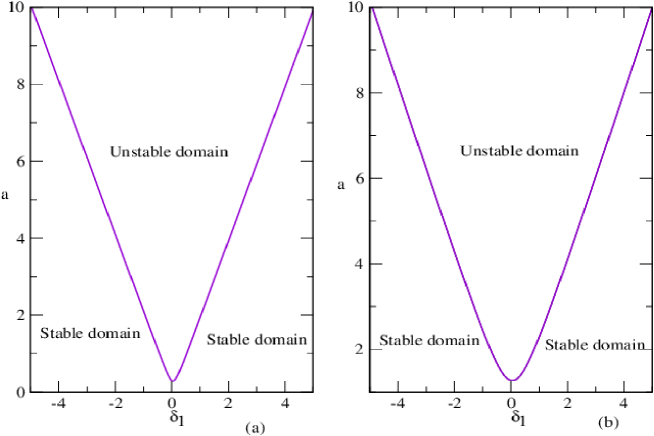
Figure 7: Stability of non-trivial solution in the space $(\delta_{1},a)$ with $\mu=0.1,c=0.5,k_{2}=0.5$, and $\tau=0.005$. (a) $b=0.1$ and (b) $b=0.35$

5 Conclusion

In this paper we have investigated the interaction of parametric excitation with time-delayed position and velocity on the parametric resonance. By the averaging method to first order, we found the equilibrium point of the system giving the amplitude and phase of vibration of the system starting. This study shows the area in which the amplitude of the vibration of the oscillator is reduced i.e. the area where vibration control is effective. We obtain also for this oscillator the Hopf bifurcation and saddle-node bifurcation for certains values of parametric parameters and time-delay. We have studied the influence of parameter $k_{2}$ which is one of parameters which modify the ordinary Rayleigh-Duffing oscillator. We applied the Routh-Hurwitz criterion for the stability study of steady-state response and we obtain the stability domain of the parametric oscillator modified Rayleigh-Duffing. We have shown clearly that the amplitude of the vibration at the primary resonance can therefore be controlled by the active control. Finally, the effects of various parameters on the control of parametric resonance have been studied.

Acknowlegments

The authors thank IMSP-UAC for financial support.

References

- [1] Nayfeh, A. H., and Mook, D. T., 1979, Nonlinear Oscillations, Wiley, New York.
- [2] Hayashi. C., 1964, Nonlinear Oscillations in Physical Systems, McGraw-Hill, New York.
- [3] Chedjou,J. C., Fostin, H. B., and Woafo, P., 1997, ”Behavior of the van der Pol Oscillator with Two External Periodic forces”,Phys. Scr., 55,pp,390-393. DEA de Physique des liquides. Paris VI- Ecole Polytechnique.
- [4] Carrol, T. L., 1995, ”Communicating With Use of filtered, Synchronized, Chaotic Signals.” IEEE Trans, Circuits syst.,I: Fundam. Theory Appl.,42,pp. 105-110.
- [5] T. Aida, K. Kawazoe, S. Toda, Vibration control of plates by plate-type dynamic vibration absorbers, J. Vib. Acoust. 117 (1995) 332–338.
- [6] Y. Okada, K. Matsuda, H. Hashitani, Self-sensing active vibration control using the moving-coil-type actuator, J. Vib. Acoust. 117 (1995) 411–415.
- [7] K. Hackl, C.Y. Yang, A.H.-D.Cheng, Stability, bifurcation and chaos of non-linear structures with control—I. Autonomous case, Int. J. Non-Linear Mech. 28 (1993) 441–454.
- [8] A.H.D. Cheng, C.Y. Yang, K. Hackl, M.J. Chajes, Stability, bifurcation and chaos of non-linear structures with control—II. Non autonomous case, Int. J. Non-Linear Mech. 28 (1993) 549–565.
- [9] Chyuan-Yow Tseng, Pi-Cheng Tung, Dynamics of a exible beam with active non-linear magnetic force, J. Vib. Acoust. 120 (1998) 39–46.
- [10] Aubin, K., Zalalutdinov, M., Alan, T., Reichenbach, R. B., Rand, R. H., Zehnder, A., Parpia, J. and Craighead, H. G., Limit Cycle Oscillations in CW Laser-Driven NEMS, Journal of Micro-electrical mechanical System 13:1018-1026, 2004.
- [11] Zalalutdinov, M., Olkhovets, A., Zehnder, A., Ilic, B., Czaplewski, D. and Craighead, H. G., Optically pumped parametric amplification for micro-mechanical systems, Applied Physics Letters 78:3142-3144, 2001.
- [12] Rand, R. H., Ramani, D. V, Keith, W. L. and Cipolla, K. M., The quadratically damped Mathieu equation and its application to submarine dynamics, Control of Vibration and Noise: New Millennium 61:39-50, 2000.
- [13] Wirkus, S., Rand, R. H. and Ruina, A., How to pump a swing, The College Mathematics Journal 29:266-275, 1998.
- [14] Zhehe Y.,Deqing M., Zichen C., Chatter suppression by parametric excitation: Model and experiments, Communications in Nonlinear Science and Numerical Simulation 330:2995-3005, 2011.
- [15] Xin-ye L., Yu-shu C., Zhi-qiang W. and Tao S., Response of parametrically excited Duffing–van der Pol oscillator with delayed feedback , Applied Mathematics and Mechanics 27:1585-1595, 2006.
- [16] M. Siewe Siewe , C. Tchawoua , S. Rajasekar, Parametric Resonance in the Rayleigh–Duffing Oscillator with Time-Delayed Feedback, Commun Nonlinear Sci Numer Simulat 17 (2012) 4485–4493.
- [17] Darya V. Verveyko and Andrey Yu. Verisokin, Application of He’s method to the modified Rayleigh equation,Discrete and Continuous Dynamical Systems, Supplement 2011, pp. 1423–1431.
- [18] Guckenheimer J., and Holmes P., Nonlinear oscillations, dynamical systems, and bifur- cations of vector fields. New York: Springer- Verlag; 1983.
- [19] J.C.Chedjou, L.K.Kana,I.Moussa,K.Kyamakya,A.Laurent, Dynamics of a quasiperiodically forced Rayleigh oscillator,Transactions of the ASME, 600/ vol.128, Sptember 2006.
- [20] B.R. Nana Nbendjo, Y. Salissou, P. Woafo, Active control with delay of catastrophic motion and horseshoes chaos in a single well Duffing oscillator, Chaos Solitons and Fractals 23 (2005) 809–816 .
- [21] R. Tchoukuegno, B.R. Nana Nbendjo, P. Woafo, Linear feedback and parametric controls of vibrations and chaotic escape in a potential, International Journal of Non-Linear Mechanics 38 (2003) 531–541.
- [22] Nayfeh A.H., (1981), Introduction to Perturbation Technique, J.Wiley, New York.
- [23] Wang, B. and Fang, Z., ‘Chaotic Oscillations of Tropical Climate: A Dynamic System Theory for ENSO’, Journal of Atmospheric Sciences 53:2786-2802, 1996.
- [24] Wang, B., Barcilon, A. and Fang, Z., ‘Stochastic Dynamics of El Nino- Southern Oscillation’, Journal of Atmospheric Sciences 56:5-23, 1999.
- [25] Zalalutdinov, M., Parpia, J.M., Aubin, K.L., Craighead, H.G., T.Alan, Zehn- der, A.T. and Rand, R.H., Hopf Bifurcation in a Disk-Shaped NEMS, Pro- ceedings of the 2003 ASME Design Engineering Technical Conferences, 19th Biennial Conference on Mechanical Vibrations and Noise, Chicago, IL, Sept. 2-6, paper no.DETC2003-48516, 2003 (CD-ROM).
- [26] Pandey, M., Rand, R. and Zehnder, A., ‘Perturbation Analysis of Entrainment in a Micromechanical Limit Cycle Oscillator’ ,Communications in Nonlinear Science and Numerical Simulation, available online, 2006.
- [27] Tina Marie Morrison, Three problems in nonlinear dynamics with 2:1 parametric excitation, Ph.D. Cornell University 2006.