Complete Analysis on the Short Distance Contribution of $B_{s}\to\ell^{+}\ell^{-}\gamma$ in Standard Model

Abstract

Using the $B_{s}$ meson wave function extracted from non-leptonic $B_{s}$ decays, we evaluate the short distance contribution of rare decays $B_{s}\to\ell^{+}\ell^{-}~{}\gamma~{}~{}(\ell=e,\mu)$ in the standard model, including all the possible diagrams. We focus on the contribution from four-quark operators which are not taken into account properly in previous researches. We found that the contribution is large, leading to the branching ratio of $B_{s}\to\ell^{+}\ell^{-}\gamma$ being nearly enhanced by a factor 3 and up to $1.7\times 10^{-8}$. The predictions for such processes can be tested in the LHC-b and B factories in near future.

I Introduction

The standard model (SM) of electroweak interaction has been remarkably successful in describing physics below the Fermi scale and is in good agreement with the most experiment data. One of the most promising processes for probing the quark-flavor sector of the SM is the rare decays. These decays, induced by the flavor changing neutral currents (FCNC) which occur in the SM only at loop level, play an important role in the phenomenology of particle physics and in searching for the physics beyond the SM Aliev97 ; Xiong01 . The observation of the penguin-induced decay $B\to X_{s}\gamma$, $B\to X_{s}\ell^{+}\ell^{-}(\ell=e,\mu)$ are in good agreement with the SM prediction, and the first evidence for the decay $B_{s}\to\mu^{+}\mu^{-}$ was confirmed at the end of 2012 Aaij:2012nna , putting strong constraints on its various extensions. Nevertheless, these processes are also important in determining the parameters of the SM and some hadronic parameters in QCD, such as the CKM matrix elements, the meson decay constant $f_{B_{s}}$, providing information on heavy meson wave functions.

Thanks to the Large Hadron Collider (LHC) at CERN we have entered a new era of particle physics. In experimental side, in the current early phase of the LHC era, the exclusive modes such as $B_{s}\to\ell^{+}\ell^{-}\gamma$ $(\ell=e,~{}\mu)$ are among the most promising decays due to their relative cleanliness and sensitivity to models beyond the SM Aliev97 ; Xiong01 . In theoretically side, since no helicity suppression exists and large branching ratios as $B_{s}\to\mu^{+}\mu^{-}$ are expected. There are mainly two kinds of contributions of $B_{s}\to\ell^{+}\ell^{-}\gamma$ in the SM: the short distance contribution which can be evaluated reliably by perturbation theory buras while the long distance QCD effects describing the neutral vector-meson resonances $\phi$ and $J/\Psi$ family Melikhov04 ; Kruger03 ; Nikitin11 . As for the short distance contribution, it is thought in previous works that a necessary work is only attaching real photon to any charged internal and external lines in the Feynman diagrams of $b\to s\ell^{+}\ell^{-}$ with statement that contributions from the attachment of photon to any charged internal propagator are regraded as to be strongly suppressed and can be neglected safely  Aliev97 ; Xiong01 ; LU06 ; Eilam97 , i.e., one can easily obtain the amplitude of $B_{s}\to\ell^{+}\ell^{-}\gamma$ by using the effective weak Hamiltonian of $b\to s\ell^{+}\ell^{-}$ and the matrix elements $\langle\gamma|\bar{s}O_{i}b|B_{s}\rangle$ $O_{i}=\gamma_{\mu}P_{L},\sigma_{\mu\nu}q^{\nu}P_{R}$ directly. Therefore contributions from the attachment of real photon with magnetic-penguin vertex to any charged external lines are of course omitted Aliev97 ; Xiong01 or stated to be negligibly small LU06 . Another contribution from loop insertion of the lower order four-quark operators are also always neglected. We note that the complete contribution seems to have been done in Melikhov04 , however it mainly concentrated on the long distance effects of the meson resonances, whereas the short distance contribution was indeed incompletely analyzed. A complete examination included all contribution to the processes in the SM is needed.

As being well known, only short-distance contribution can be reliably predicted, and it is more important than the long-distance contribution from the resonances which is actually excluded partly by setting cuts in experimental measurements. Recently we showed that the contributions from the attachment of real photon with magnetic-penguin vertex to any charged external lines can enhance the branching ratios of $B_{s}\to\ell^{+}\ell^{-}\gamma$ by a factor about 2 Wang:2012na .

In this letter, we will extend our previous studies and use the $B_{s}$ meson wave function extracted from non-leptonic $B_{s}$ decays bs to revaluate the short distance contribution from the all categories of diagrams of $B_{s}\to\ell^{+}\ell^{-}\gamma$ decays. Special attention will be payed on the contribution from the four-quark operators, and a comparative study with previous work will be discussed. The paper are organized in the following, in sec. II, we analyse the full short distance contribution and present detail calculation of exclusive decays $B_{s}\to\ell^{+}\ell^{-}\gamma$. The numerical results and the comparative study are given in sec. III, and the conclusions are given in sec. IV.

II Complete analysis on short distance contributions

In order to simplify the decay amplitude for $B_{s}\to\ell^{+}\ell^{-}\gamma$, we have to utilize the $B_{s}$ meson wave function, which is not known from the first principal and model depended. Fortunately, many studies on non-leptonic $B$ bdecay ; cdepjc24121 and $B_{s}$ decays bs have constrained the wave function strictly. It was found that the wave function has form

$$\Phi_{B_{s}}=(\not\!p_{B_{s}}+m_{B_{s}})\gamma_{5}~{}\phi_{B_{s}}({x}),$$ (1)

where the distribution amplitude $\phi_{B_{s}}(x)$ can be expressed as form :

$$\phi_{B_{s}}(x)=N_{B_{s}}x^{2}(1-x)^{2}\exp\left(-\frac{m_{B}^{2}\ x^{2}}{2\omega_{b_{s}}^{2}}\right)$$ (2)

with $x$ being the momentum fractions shared by $s$ quark in $B_{s}$ meson. The normalization constant $N_{B_{s}}$ can be determined by comparing

$$\langle 0\left|\bar{s}\gamma^{\mu}\gamma_{5}b\right|B_{s}\rangle=iN_{c}\int_{0}^{1}\phi_{B_{s}}(x)dx{\rm Tr}\left[\gamma^{\mu}\gamma_{5}(\not\!p_{B_{s}}+m_{B_{s}})\gamma_{5}\right]dx=-4N_{c}ip_{B_{s}}^{\mu}\int_{0}^{1}\phi_{B_{s}}(x)dx$$ (3)

with $N_{c}$ being the number of quarks and

$$\langle 0\left|\bar{s}\gamma^{\mu}\gamma_{5}b\right|B_{s}\rangle=-if_{B_{s}}p_{B_{s}}^{\mu},$$ (4)

the $B$ meson decay constant $f_{B_{s}}$ is thus determined by the condition

$$\int_{0}^{1}\phi_{B_{s}}(x)dx=\frac{1}{4N_{c}}f_{B_{s}}.$$ (5)

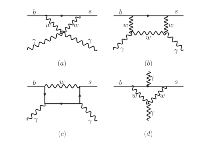
Figure 1: Feynman diagrams without effective vertex of $b\to s\gamma$ contribution to $B_{s}\to\gamma\gamma$.

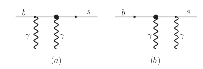
Figure 2: Feynman diagrams with effective vertex of $b\to s\gamma$ contribution to $B_{s}\to\gamma\gamma$ . The black dot stands for the magnetic-penguin operator $O_{7}$

Let us start with the quark level processes $B_{s}\to\ell^{+}\ell^{-}\gamma$ which are subject to the QCD corrected effective weak Hamiltonian. The general effective Hamiltonian that describes $b\to s$ transition is given by

$${\cal H}_{eff}=-\frac{4G_{F}}{\sqrt{2}}V_{tb}V^{*}_{ts}\sum\limits_{j=1}^{10}C_{j}(\mu)O_{j}(\mu),$$ (6)

where $O_{j}$ ($j=1,\dots,6$) stands for the four-quark operators, and the forms and the corresponding Wilson coefficients $C_{i}$ can be found in Ref. Misiak93 .

Generally, to describe all the short distance of the process $B_{s}\to\ell^{+}\ell^{-}\gamma$, new effective operators for $b\to s\gamma\gamma$ which are not included in (6) should be introduced. Corresponding feynman diagrams without and with effective vertex $b\to s\gamma$ are shown in FIG. 1 and FIG. 2, respectively. When connect di-lepton line to one $\gamma$, operator $b\to s\gamma\gamma$ may contribute to $B_{s}\to\ell^{+}\ell^{-}\gamma$. Contributions from the such kind of diagrams with a photon attaching from internal charged lines to $B_{s}\to\ell^{+}\ell^{-}\gamma$ are usually regraded as to be strongly suppressed by a factor $m_{b}^{2}/m_{W}^{2}$ thus can be neglected safely  Aliev97 ; Xiong01 ; LU06 ; Eilam97 . However, as pointed out in Dong , the conclusion of this is correct, but the explanation is not as what it is described. Here we address the reason more clearly: the contribution from diagrams FIG. 1 (a) and FIG. 1 (b) are not suppressed. When applying effective vertex of $b\to s\gamma$ to describe $b\to s\gamma\gamma$ as shown in FIG. 2, internal quarks in the effective vertex are off-shell and such off-shell effects are also not suppressed. We have proven that the such two non-suppressed effects in FIG. 1 and FIG. 2 cancel each other exactly Dong . Therefore we can use the effective operators listed in Eq. (6) for on-shell quarks to calculate the total short distance contributions of $B_{s}\to\ell^{+}\ell^{-}\gamma$ in SM safely.

The Feynmann diagrams contributing to $B_{s}\to\ell^{+}\ell^{-}\gamma$ at parton level can then be classified into three kinds as follows:

1. Attaching a real photon to any charged external lines in the Feynman diagrams of $b\to s\ell^{+}\ell^{-}$;

2. Attaching a virtual photon to any charged external lines in the Feynman diagrams of $b\to s\gamma$ with virtual photon into lepton pairs;

3. Attaching two photon to any charged external lines in the Feynman diagrams of four-quark operators with one of two photon into lepton pairs.

Note that the third contribution is not considered in the previous studies except for Ref. Melikhov04 which is the focus of this paper and will show the detail in the following. We also will discuss these contributions seperatly.

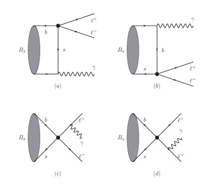
Figure 3: Feynman diagrams that contribute to the matrix elements $B_{s}\to\ell^{+}\ell^{-}\gamma$ with the contribution of $O_{7},~{}O_{9},~{}O_{10}$ in tree level.

II.1 External real photon contributions

The Feynman diagrams of the first kind of contributions are shown in FIG. 3. As the contribution from the FIG. 3 (c) and (d) with photon attached to external lepton lines, considering the fact that (i) being a pseudoscalar meson, $B_{s}$ meson can only decay through axial current, so the magnetic penguin operator $O_{7}$ ’s contribution vanishes; (ii) the contribution from operators $O_{9},\ O_{10}$ has the helicity suppression factor $m_{\ell}/m_{B_{s}}$, so for light lepton electron and muon, we can neglect their contribution safely. These diagrams in FIG. 3 (a) and (b) are always regarded as the dominant contributions, and they have been considered by using the light cone sum rule Aliev97 ; Xiong01 , the simple constituent quark model Eilam97 , and the B meson distribution amplitude extracted from non-leptonic B decays LU06 . We rewrite the amplitude of $B_{s}\to\ell^{+}\ell^{-}\gamma$ at meson level as Wang:2012na :

$$A_{\rm I} = iN_{c}Gee_{d}\frac{1}{p_{B_{s}}\cdot k}\biggl{\{}\left[C_{1}i\epsilon_{\alpha\beta\mu\nu}p^{\alpha}_{B_{s}}\varepsilon^{\beta}{k^{\nu}}+C_{2}p_{B_{s}}^{\nu}(\varepsilon_{\mu}k_{\nu}-k_{\mu}\varepsilon_{\nu})\right]\bar{\ell}\gamma^{\mu}{\ell}$$ (7)

$$+C_{10}\left[C_{+}i\epsilon_{\alpha\beta\mu\nu}p^{\alpha}_{B_{s}}\varepsilon^{\beta}{k^{\nu}}+C_{-}p_{B_{s}}^{\nu}(\varepsilon_{\mu}k_{\nu}-k_{\mu}\varepsilon_{\nu})\right]\bar{\ell}\gamma^{\mu}\gamma_{5}\ell\biggl{\}}.$$

The form factors in Eq. (7) are found to be:

$$C_{1} = C_{+}\left(C_{9}^{eff}-2\frac{m_{b}m_{B_{s}}}{q^{2}}C_{7}^{eff}\right),$$

$$C_{2} = C_{9}^{eff}C_{-}-2\frac{m_{b}m_{B_{s}}}{q^{2}}C_{7}^{eff}C_{+},$$ (8)

with the constant $G=\alpha_{em}G_{F}V_{tb}V_{ts}^{*}/(\sqrt{2}\pi)$, and

$$C_{\pm}=\int_{0}^{1}\left(\frac{1}{x}\pm\frac{1}{y}\right)\phi_{B_{s}}(x)dx.$$ (9)

The expression in Eq. (7) can be compared with Ref. LU06 .

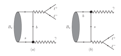
Figure 4: Feynman diagrams of $b\to s\gamma$ with virtual photon into lepton pairs .

II.2 External virtual photon contributions

The Feynman diagrams of the second kind of contributions are shown in FIG. 4. Contributions from the kind of diagrams are always neglected Aliev97 ; Xiong01 or stated to be negligibly small LU06 . Note the $B_{s}$ meson wave functions used in this work and Ref. LU06 are both from non-leptonic $B_{s}$ decays. However, as mentioned in the introduction the authors of Ref.  LU06 did not present the expression of the contribution from FIG. 4 and only stated the contribution is numerical negligibly small. But such statement seems to be questionable, for that the pole of propagator of the charged line attached by photon may enhance the decay rate greatly which make some diagrams can not be neglected in the calculation. In these two diagrams, photon of the magnetic-penguin operator is real, thus its contribution to $B_{s}\to\ell^{+}\ell^{-}\gamma$ is different from the first kind contributions. We get the amplitude Wang:2012na :

$$A_{\rm II}=i2N_{c}Gee_{d}C_{7}^{eff}\frac{m_{b}m_{B_{s}}}{q^{2}}\frac{1}{p_{B_{s}}\cdot q}\overline{C}_{+}\left[k_{\mu}q\cdot\epsilon-\epsilon_{\mu}k\cdot q-i\epsilon_{\mu\nu\alpha\beta}\epsilon^{\nu}k^{\alpha}q^{\beta}\right]\left[\bar{\ell}\gamma^{\mu}\ell\right],$$ (10)

with coefficients $\overline{C_{+}}$ obtained by a replacement:

$$\overline{C}_{+} = C_{+}(x\to\bar{x}=x-z-i\epsilon;~{}y\to\bar{y}=y-z-i\epsilon)$$ (11)

$$= N_{B}\int_{0}^{1}dx({\frac{1}{x-z-i\epsilon}}+{\frac{1}{1-x-z-i\epsilon}})x^{2}(1-x)^{2}\exp\left[-\frac{m_{B_{s}}^{2}}{2\omega_{B_{s}}^{2}}x^{2}\right],$$

where $z=\frac{q^{2}}{2p_{B_{s}}\cdot q}$ and the first, second term in (11) denotes the contribution from FIG. 4 (a) and (b) respectively. Note that the contribution from FIG. 3 (a) is much larger than (b) since $m_{B_{s}}\ll\omega_{B_{s}}$ (see next section) which is very easily understood in sample constituent quark model Eilam97 , i.e., $\phi_{B_{s}}(x)=\delta(x-m_{s}/m_{B_{s}})$. However, the contributions from Fig.4 (a) and (b) are comparable, and pole in $\overline{C_{+}}$ corresponds to the pole of the quark propagator when it is connected by the off-shell photon propagator. Thus the $\overline{C_{+}}$ term may enhance the decay rate of $B_{s}\to\ell^{+}\ell^{-}\gamma$ and its analytic expression reads

$$\overline{C}_{+} = 2N_{B_{s}}\pi iz^{2}(1-z)^{2}\exp\left[-\frac{m_{B_{s}}^{2}}{2\omega_{B_{s}}^{2}}z^{2}\right]$$ (12)

$$+ N_{B_{s}}\int_{0}^{1}dx({\frac{1}{x+z}}-{\frac{1}{1+x-z}})x^{2}(1+x)^{2}\exp\left[-\frac{m_{B_{s}}^{2}}{2\omega_{B_{s}}^{2}}x^{2}\right]$$

$$- N_{B_{s}}\int_{-1}^{1}\left(\frac{1}{\frac{1}{x}-z}+\frac{1}{1-\frac{1}{x}-z}\right)\frac{dx}{x^{4}}(1-\frac{1}{x})^{2}\exp\left[-\frac{m_{B_{s}}^{2}}{2\omega_{B_{s}}^{2}}\frac{1}{x^{2}}\right].$$

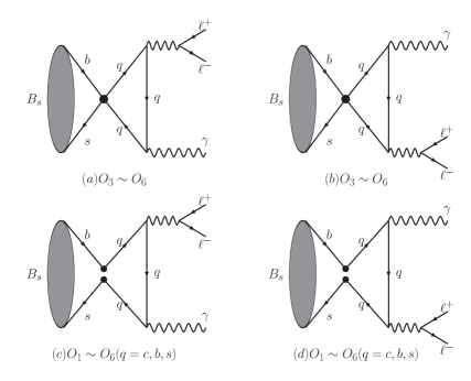
Figure 5: Feynman diagrams that contribute to the process $B_{s}\to\ell^{+}\ell^{-}\gamma$ with possible insertion of $O_{1}$ to $O_{6}$ in loop level .

II.3 Quark weak annihilation contributions

Now we focus on the contributions from the diagrams for the four-quark operators which are not considered properly in previous works. The Feynman diagrams of the third kind of contribution are shown in FIG. 5. The operator $O_{7}$ is high order than four-quark operator $O_{1}-O_{6}$, thus the contribution of loop diagram with operator $O_{1}-O_{6}$ insertion should be comparable with the tree level electro-weak penguin $O_{7}-O_{10}$ contributions listed above. To calculate the leading order matrix elements of $b\to s\gamma^{\ast}\gamma$ shown in FIG. 5, we express the decay amplitude for $b(p_{b})\to s(p_{s})\gamma^{\ast}(k_{1})\gamma(k_{2})$ as

$$A_{\rm III}(b\to s\gamma^{*}\gamma)=i\frac{4G_{F}}{\sqrt{2}}V_{tb}V^{*}_{ts}\frac{e^{2}}{16\pi^{2}}\bar{s}(p_{s})T_{\mu\nu}b(p_{b})\epsilon^{\mu}(k_{1})\epsilon^{\nu}(k_{2}),$$ (13)

where $p_{b,s},k_{1,2}$ denotes the momentum of quarks and photon respectively, $\epsilon$ is the vector polarization of photon. We split the tensor $T^{\mu\nu}$ into the momentum odd and even power terms for simplification. Keeping our physics goal in mind, Without loss of generality we assume that photon with momentum $k_{1}$ is virtual and drop the terms proportional to $k_{2}^{\nu}$ in the expressions. After straight calculation, we obtain

$$T_{\mu\nu}^{\rm odd}(q) = e_{q}^{2}\left\{\frac{1}{k_{1}k_{2}}\left[i\epsilon_{\nu\alpha\beta\lambda}\gamma^{\lambda}\gamma_{5}k_{1}^{\alpha}k_{2}^{\beta}\left[k_{1{\mu}}f_{2}(q)-k_{2\mu}f_{+}(q)\right]+i\epsilon_{\mu\alpha\beta\lambda}\gamma^{\lambda}\gamma_{5}k_{1}^{\alpha}k_{2}^{\beta}k_{1{\nu}}f_{+}(q)\right]\right.$$ (14)

$$\left.+i\epsilon_{\mu\nu\alpha\beta}\gamma^{\beta}\gamma_{5}[k_{1}^{\alpha}f_{+}(q)-k_{2}^{\alpha}f_{-}(q)]\right\},$$

$$T_{\mu\nu}^{\rm even}(q) = -2\frac{e_{q}^{2}}{m_{q}}\left\{(k_{1\nu}k_{2\mu}-k_{1}k_{2}g_{\mu\nu})\left[f_{3}(q)+(1-\frac{4}{z_{q}})f^{\prime}_{1}(q)\right]+i\epsilon_{\mu\nu\alpha\beta}\gamma_{5}k_{1}^{\alpha}k_{2}^{\beta}f_{1}^{\prime}(q)\right\},$$ (15)

where $q$ denotes the quark in the internal line which two photons are attached and and $e_{q}$ is the number of electrical charge of the quark. The loop functions appearing in (15) have forms as

$$f_{\pm}(q) = \frac{1}{2}+\frac{1}{z_{q}}\int_{0}^{1}\ln g(z_{q},u_{q},x)\frac{\mathrm{d}x}{x}\mp\frac{u_{q}}{2z_{q}}\int_{0}^{1}\ln g(z_{q},u_{q},x),$$

$$f_{1}(q) = \frac{1}{2}[f_{+}(q)+f_{-}(q)],\ f_{2}(q)=\frac{z_{q}}{2u_{q}}[f_{+}(q)-f_{-}(q)],$$

$$f_{3}(q) = \frac{2}{z_{q}}-\frac{2u_{q}}{z_{q}^{2}}\int_{0}^{1}\mathrm{ln}g(z_{q},u_{q},x)\mathrm{d}x,$$

$$g(z,u,x) = \frac{1-(u+z)x(1-x)}{1-ux(1-x)},$$ (16)

with $f_{1}^{\prime}(q)=\frac{1}{2}-f_{1}(q)$, $z_{q}=\frac{2k_{1}\cdot k_{2}}{m_{q}^{2}}$ and $u_{q}=\frac{k_{1}^{2}}{m_{q}^{2}}$. Writing the amplitude in this ways, one can infer easily that for example, when operators $O_{j}$ ($j=1,\dots,4$) are inserted, only $T_{\mu\nu}^{\rm odd}$ part can contribute to $b\to s\gamma\gamma$ while the process receives both parts contributions as $O_{5,6}$ are inserted. It is also easily obtained the similar result for the on-shell photons as in Ref. Cao01 by setting $u_{q}=0$ .

With the amplitude of $b\to s\gamma^{*}\gamma$ and $B_{s}$ wave function ready, we write the total contribution from FIG. 5 to exclusive decay of $B_{s}(p_{B_{s}})\to\gamma(k)\ell^{+}\ell^{-}$ as

$$A_{\rm III}=-2ie\frac{f_{B_{s}}G}{q^{2}}\sum\limits_{j=1}^{6}C_{j}(m_{b})\left[T_{1}^{j}p_{B_{s}}^{\nu}(\epsilon_{\nu}k_{\mu}-\epsilon_{\mu}k_{\nu})+T_{2}^{j}i\epsilon_{\mu\nu\alpha\beta}p_{B_{s}}^{\alpha}k^{\beta}\epsilon^{\nu}\right][\bar{\ell}\gamma^{\mu}\ell],$$ (17)

with the form factors given by

$$T_{1}^{1} = T_{1}^{2}=T_{1}^{3}=T_{1}^{4}=0;$$

$$T_{2}^{1} = N_{c}T_{2}^{2}=N_{c}e_{u}^{2}f_{1}(\bar{z}_{c},t);$$

$$T_{2}^{3} = N_{c}\left\{\sum\limits_{q=u,d,s,c,b}e_{q}^{2}f_{1}(\bar{z}_{q},t)+e_{d}^{2}[f_{1}(\bar{z}_{b},t))+f_{1}(\bar{z}_{s},t)]\right\}$$

$$T_{2}^{4} = \sum\limits_{q=u,d,s,c,b}e_{q}^{2}f_{1}(\bar{z}_{q},t)+e_{d}^{2}N_{c}\left[f_{1}(\bar{z}_{b},t))+f_{1}(\bar{z}_{s},t)\right]$$

$$T_{1}^{5} = =\frac{1}{N_{c}}T_{1}^{6}=2e_{d}^{2}\left\{\frac{1}{\bar{z}_{b^{1/2}}}\left[f_{3}(\bar{z}_{b},t)+(1-\frac{4\bar{z}_{b}}{1-t})(\frac{1}{2}-f_{1}(\bar{z}_{b},t))\right]-(b\to s)\right\};$$

$$T_{2}^{5} = =-N_{c}\sum\limits_{q=u,d,s,c,b}e_{q}^{2}f_{1}(\bar{z}_{q},t)-2e_{d}^{2}\left[\frac{1}{\bar{z}_{b^{1/2}}}(\frac{1}{2}-f_{1}(\bar{z}_{b},t))+(b\to s)\right];$$

$$T_{2}^{6} = -\sum\limits_{q=u,d,s,c,b}e_{q}^{2}f_{1}(\bar{z}_{q},t)-2N_{c}e_{d}^{2}\left[\frac{1}{\bar{z}_{b^{1/2}}}(\frac{1}{2}-f_{1}(\bar{z}_{b},t))+(b\to s)\right],$$ (18)

where $q^{2}$ in Eq. (17) is the invariant mass square of lepton pair. The functions can be obtained directly from (16) by redefined parameters $\bar{z}_{q}=m_{q}^{2}/m^{2}_{B_{s}}$, $t=q^{2}/m^{2}_{B_{s}}$,

$$f_{1}(\bar{z},t) = \frac{1}{2}+\frac{\bar{z}}{1-t}\int_{0}^{1}\frac{dx}{x}\ln[\frac{\bar{z}-x(1-x)}{\bar{z}-tx(1-x)}],$$ (19)

$$f_{3}(\bar{z},t) = \frac{2\bar{z}}{1-t}\left\{1-\frac{t}{1-t}\int_{0}^{1}{dx}\ln[\frac{\bar{z}-x(1-x)}{\bar{z}-tx(1-x)}]\right\},$$ (20)

with explicit formula needed in calculation given by

$$\int_{0}^{1}\frac{dy}{y}\ln[1-vy(1-y)-i\epsilon] = \left\{\begin{array}[]{cc}-2\mathrm{arctan^{2}\sqrt{\frac{v}{4-v}}}&{\rm for}~{}v<4;\\ -\frac{\pi^{2}}{2}-2i\pi\ln\frac{\sqrt{v}+\sqrt{v-4}}{2}+2\ln^{2}\frac{\sqrt{v}+\sqrt{v-4}}{2}&{\rm for}~{}v>4,\\ \end{array}\right.,$$ (23)

$$\int_{0}^{1}dy\ln[1-vy(1-y)-i\epsilon] = -2+|1-x|^{1/2}\left\{\begin{array}[]{cc}\ln\left|\frac{1+\sqrt{1-x}}{1-\sqrt{1-x}}\right|-i\pi&{\rm for}~{}x=4/v<1;\\ 2\arctan\frac{1}{\sqrt{x-1}}&{\rm for}~{}x=4/v>1.\end{array}\right.$$ (26)

From Eq. (17) it is clear that the contribution from four-quark operators to $B_{s}\to\gamma\ell^{+}\ell^{-}$ has the similar expression as that from magnetic-penguin operator with real photon to $B_{s}\to\ell^{+}\ell^{-}\gamma$. Thus the total matrix element for the decay $B_{s}\to\ell^{+}\ell^{-}\gamma$ including contributions from three kinds of diagrams can be obtained easily by a shift to the form factors:

$$\overline{C}_{1} = C_{+}\left[C_{9}^{eff}-\frac{2m_{b}m_{B_{s}}}{q^{2}}C_{7}^{eff}\left(1+\frac{p_{B_{s}}\cdot k}{p_{B_{s}}\cdot q}\right)\right]-2\frac{p_{B_{s}}\cdot k}{q^{2}}\frac{f_{B_{s}}}{e_{d}}\sum\limits_{j=1}^{6}C_{j}T_{2}^{j},$$ (27)

$$\overline{C}_{2} = C_{9}^{eff}C_{-}-\frac{2m_{b}m_{B_{s}}}{q^{2}}C_{7}^{eff}C_{+}\left(1+\frac{p_{B_{s}}\cdot k}{q^{2}}\right)+2\frac{p_{B_{s}}\cdot k}{q^{2}}\frac{f_{B_{s}}}{e_{d}}\sum\limits_{j=1}^{6}C_{j}T_{1}^{j}.$$ (28)

Finally, we get the differential decay width versus the photon energy $E_{\gamma}$,

$$\frac{d\Gamma}{dE_{\gamma}} = \frac{\alpha_{em}^{3}{G^{2}_{F}}}{108\pi^{4}}|V_{tb}V^{*}_{ts}|^{2}(m_{B_{s}}-2E_{\gamma})E_{\gamma}\left[|\overline{C}_{1}|^{2}+|\overline{C_{2}}|^{2}+C_{10}^{2}(|C_{+}|^{2}+|C_{-}|^{2})\right].$$ (29)

III Results and discussions

The decay branching ratios can be easily obtained by integrating over photon energy. In the numerical calculations, we use the following parameters PDG2012 :

$$\alpha_{em}=\frac{1}{137},~{}G_{F}=1.166\times 10^{-5}{\rm GeV}^{-2},~{}m_{b}=4.2{\rm GeV},$$

$$|V_{tb}|=0.999,~{}|V_{ts}|=0.04,~{}|V_{td}|=0.0084$$

$$m_{B_{s}}=5.37{\rm GeV},~{}\omega_{B_{s}}=0.5,~{}f_{B_{s}}=0.24{\rm GeV},~{}\tau_{B_{s}}=1.47\times 10^{-12}s.$$

$$m_{B_{d}^{0}}=5.28{\rm GeV},~{}\omega_{B_{d}}=0.4,~{}f_{B_{d}}=0.19{\rm GeV},~{}\tau_{B_{d}}=1.53\times 10^{-12}s.$$

The ratios of $B_{s}\to\gamma\ell^{+}\ell^{-}$ are shown in Table 1 together with results of $B_{d,s}\to\gamma\ell^{+}\ell^{-}$ from this work and our previous research for comparison. The errors shown in the Table 1 comes from the heavy meson wave function, by varying the parameter $\omega_{B_{d}}=0.4\pm 0.1$, and $\omega_{B_{s}}=0.5\pm 0.1$ LU06 . Note that, the predicted branching ratios receive errors from many parameters, such as parameters meson decay constant, meson and quark masses.

Table 1: Comparison of branching ratios in unit of $10^{-9}$ with previous calculations

Branching Ratios	Results
($\times 10^{-9}$)	The first kind of diagrams	The first two kind of diagrams	Included all diagrams
$B_{s}\to\gamma\ell^{+}\ell^{-}$	$5.16_{-1.38}^{+2.42}$	$10.2_{-2.51}^{+4.11}$	$17.36_{-2.63}^{+4.55}$
$B_{d}^{0}\to\gamma\ell^{+}\ell^{-}$	$0.21_{-0.06}^{+0.14}$	$0.40_{-0.13}^{+0.26}$	$0.53_{-0.12}^{+0.26}$

From the numerical results we conclude that unlike in decay $B\to X_{s}\gamma\gamma$ where the four-quark operators just contribute a few percent to the branching ratio Cao01 , our numerical result shows that contribution from the four-quark operators to $B_{s}\to\gamma\ell^{+}\ell^{-}$ is large. It can be understood as follows:

1. As pointed out in Ref. LU06 , the radiative leptonic decays are very sensitive probes in extracting the heavy meson wave functions;

2. Values of the Wilson coefficients $C_{j}(m_{b})$ ($j=3,\dots,6$) are at order of $10^{-2}$, indicating that contribution to the corresponding operators via $T^{j}$ is less important compared with those from $O_{1,2}$;

3. From Eq. (18), one can infer easily that the four-quarks contribution to the form factors in (28) have coefficient $(N_{c}C_{1}+C_{2})T_{2}^{2}f_{B_{s}}/e_{d}$ while the contribution from magnetic-penguin operator with real photon, $m_{b}m_{B_{s}}/(p_{B_{s}}\cdot q)C_{7}^{eff}C_{+}$. Note $(N_{c}C_{1}+C_{2})/e_{d}$ and $C_{7}^{eff}$ can be comparable and have the same sign in $\overline{C}_{1}$ and opposite sign in $\overline{C}_{2}$. However, with $T_{1}^{j}=0$ for $j=1,2$ thus comparable contribution studied in this work and in Ref. Wang:2012na is expected, leading to enhancement of branching ratios of $B_{s}\to\gamma\ell^{+}\ell^{-}$ when new diagrams are taken into account.

4. The predicted short-distance contributions from quark weak annihilation as well as the magnetic-penguin operator with real photon to the exclusive decay are large, and the branching ratios of $B_{s}\to\ell^{+}\ell^{-}\gamma$ are enhanced nearly by a factor 3 compared with that only contribution from magnetic-penguin operator with virtual photon and up to $1.7\times 10^{-8}$, implying the search of $B_{s}\to\ell^{+}\ell^{-}\gamma$ can be achieved in near future.

5. Due to the large contributions from magnetic-penguin operator with real photon and quark weak annihilation , the form factors for matrix elements $\langle\gamma|\bar{s}\gamma_{\mu}(1-\gamma_{5})b|B_{s}\rangle$ and $\langle\gamma|\bar{s}\sigma_{\mu\nu}(1\pm\gamma_{5})q^{\nu}b|B_{s}\rangle$ as a function of dilepton mass squared $q^{2}$ are complex and not as simple as $1/(q^{2}-q_{0}^{2})^{2}$ where $q_{0}^{2}$ is constant Eilam95 . The $B_{s}\to\gamma$ transition form factors predicted in this works have also some differences from those in Ref. Melikhov04 ; Kruger03 ; Nikitin11 . For instance, Ref. Kruger03 predicted the form factors $F_{TV}(q^{2},0)$, $F_{TA}(q^{2},0)$ induced by tensor and pseudotensor currents with direct emission of the virtual photon from quarks are only equal at maximum photon energy, whereas the corresponding formula in this work have the same expression as $-\frac{e_{d}N_{c}m_{B_{s}}}{p_{B_{s}}\cdot k}C_{+}\propto 1/(q^{2}-q_{0}^{2})$ in Eq. (7). Furthermore, the form factors are larger than previous predictions.

To clarify things more clear, we think it is necessary to present a few more comments about the calculation of Ref. Melikhov04 , as mentioned in introduction. In order to estimate the contribution of direct emission of the real photon from quarks, the authors of Ref. Melikhov04 calculated the form factors $F_{TA,TV}(0,q^{2})$ by including the short-distance contribution in $q^{2}\to 0$ limit and additional long-distance contribution from the resonances of vector mesons such as $\rho^{0}$, $\omega^{0}$ for $B_{d}$ decay and $\phi$ for $B_{s}$ decay. Obviously, this means the short-distance contributions were not appropriately taken into account. Moreover, if $F_{TA,TV}(0,q^{2})=F_{TA,TV}(0,0)$ stands for the short distance contribution, it seems to double counting since in this case photons emitted from magnetic-penguin vertex and quark lines directly are not able to be distinguished.

We also note that for contribution from the weak annihilation the authors of Ref. Melikhov04 only took into account $u$ and $c$ quarks in the loop by axial anomaly as the long distance contribution, they concluded that the anomalous contribution is suppressed by a power of a heavy quark mass. We believe that only anomalous contribution to account contribution from the weak annihilation is insufficient. Our numerical result shows that the contributions from weak-annihilation diagrams are large and can not be neglected.

IV Conclusion

In summary, we evaluated short distance calculation of the rare decays $B_{s}\to\gamma\ell^{+}\ell^{-}$ in the SM, including contributions from all four kinds of diagrams. We focus on the contribution from four-quark operators which are not taken into account properly in previous researches. We found that the contributions are large, leading to the branching ratio of $B_{s}\to\ell^{+}\ell^{-}\gamma$ being nearly enhanced by a factor 3. In the current early phase of the LHC era, the exclusive modes with muon final states are among the most promising decays. Although there are some theoretical challenges in calculation of the hadronic form factors and non-factorable corrections, with the predicted branching ratio at order of $10^{-8}$, $B_{s}\to\mu^{+}\mu^{-}\gamma$ can be expected as the next goal after $B_{s}\to\mu^{+}\mu^{-}$ since the final states can be identified easily and the branching ratios are large. Experimentally, $B_{s}\to\mu^{+}\mu^{-}\gamma$ mode is one of the main backgrounds to $B_{s}\to\mu^{+}\mu^{-}$, and thus it is already taken into account in $B_{s}\to\mu^{+}\mu^{-}$ searches Aaij:2012nna . Our predictions for such processes can be tested in the LHC-b and B factories in near future.

References

• (1) T.M. Aliev, A. Ozpineci, M. Savci, Phys. Rev. D 55,7059 (1997).
• (2) Z. Heng, R. J. Oakes, W. Wang, Z.H. Xiong and J. M. Yang, Phys. Rev. D 77, 095012 (2008); G. Lu, Z.H. Xiong, Y. Cao, Nucl.Β Phys.Β B 487, 43 (1997); Z.H.Β Xiong, J.Β M.Β Yang, Nucl.Β Phys.Β B 602, 289 (2001) and Nucl.Phys. B 628, 193 (2002); G. LuΒ et. al., Phys. Rev. D 54, 5647 (1996); Z. H. Xiong, High Energy Phys. Nucl. Phys. 30, 284 (2006).
• (3) RAaij et al. [LHCb Collaboration], Phys.Β Rev.Β Lett.Β  110, 021801 (2013) [arXiv:1211.2674 [Unknown]].
• (4) G. Buchalla, A. J. Buras, M. E. Lautenbacher, Rev. Mod. Phys. Vol 68, No. 4, 1125.
• (5) D. Melikhov and N. Nikitin, Phys. Rev. D70,114028, (2004).
• (6) F.Kruger and D.Melikhov, Phys.Rev. D67, 034002 (2003);
• (7) N. Nikitin, I. Balakireva, and D. Melikhov, arXiv:1101.4276v1 [hep-ph]; C.Q. Geng, C.C. Lih, W.M. Zhang, Phys.Rev. D62, 074017 (2000); Y. Dincer and L.M. Sehgal, Phys.Lett. B521, 7 (2001); S.Descotes-Genon, C.T. Sachrajda, Phys.Lett. B557, 213 (2003).
• (8) G. Eilam, C.-D. LΓΌ and D.-X. Zhang, Phys. Lett. B 391, 461 (1997); G.Β Erkol and G.Β Turan, Phys.Β Rev.Β D 65, 094029 (2002).
• (9) J.-X. Chen, Z.Y. Hou , C.-D. LΓΌ, Commun. Theor. Phys. 47, 299 (2007).
• (10) W.Β Wang, Z.Β -H.Β Xiong and S.Β -H.Β Zhou, arXiv:1207.1978 [hep-ph].
• (11) Y.Β Li, C.D.Β LΓΌ, Z.J.Β Xiao, and X.Q.Β Yu, Phys. Rev. D 70, 034009 (2004); X.QΒ Yu, Y.Β Li and C.D.Β LΓΌ, Phys. Rev. D 71, 074026 (2005) and 2006 Phys. Rev. D 73, 017501.
• (12) C.-D.Β LΓΌ, K.Β Ukai and M.-Z.Β Yang, Phys. Rev. D 63, 074009 (2001); Y.-Y.Β Keum, H.-n.Β Li and A.I.Β Sanda, Phys. Lett. B 504, 6 (2001), Phys. Rev. D 63, 054008 (2001); H.-n. Li, 2001 Phys. Rev. D 64, 014019 (2001); S.Β Mishima, Phys. Lett. B 521, 252 (2001); C.-H.Β Chen, Y.-Y.Β Keum, and H.-n.Β Li, Phys. Rev. D64, 112002 (2001) and Phys. Rev. D 66, 054013 (2002).
• (13) C.D.Β LΓΌ, Eur. Phys. J. C 24, 121 (2002) and Phys. Rev. D 68, 097502 (2003); Y.-Y.Β Keum and A.I.Β Sanda, Phys. Rev. D 67, 054009 (2003); Y.-Y.Β Keum, et al., Phys. Rev. D 69, 094018 (2004); J.Β Zhu, Y.L.Β Shen and C.D.Β LΓΌ, 2005 Phys. Rev. D 72, 054015, and Eur. Phys. J. C41, 311 (2005); Y.Β Li and C.D.Β LΓΌ, Phys. Rev. D73, 014024 (2006); C.D.Β LΓΌ, M.Β Matsumori, A.I.Β Sanda, and M.Z.Β Yang, Phys. Rev. D 72, 094005 (2005).
• (14) C.-D.Β LΓΌ and M.-Z.Β Yang, 2003 Eur. Phys. J. C 28, 515.
• (15) M. Misiak, Nucl. Phys. B 393, 23 (1993).
• (16) F.L. Dong, W.Y. Wang, and Z.H. Xiong, Chin. Phys. C 35, 6 (2011).
• (17) J.J. Cao, Z.J. Xiao and G.R. Lu, Phys. Rev. D 64, 014012 (2001); L. Reina, G. Ricciardi, and A. Soni, Phys. Rev. D 56, 5805 (1997).
• (18) G. Eilam, I. Halperin and R. R. Mendel, Phys. Lett. B 361, 137 (1995).
• (19) K. Nakamura et al. (Particle Data Group), J. Phys. G 37, 075021 (2010) and 2011 partial update for the 2012 edition.