DISTRIBUTED ALLOCATION OF MOBILE SENSING SWARMS IN GYRE FLOWS

Zusammenfassung

We address the synthesis of distributed control policies to enable a swarm of homogeneous mobile sensors to maintain a desired spatial distribution in a geophysical flow environment, or workspace. In this article, we assume the mobile sensors (or robots) have a “map” of the environment denoting the locations of the Lagrangian coherent structures or LCS boundaries. Using this information, we design agent-level hybrid control policies that leverage the surrounding fluid dynamics and inherent environmental noise to enable the team to maintain a desired distribution in the workspace. We discuss the stability properties of the ensemble dynamics of the distributed control policies. Since realistic quasi-geostrophic ocean models predict double-gyre flow solutions, we use a wind-driven multi-gyre flow model to verify the feasibility of the proposed distributed control strategy and compare the proposed control strategy with a baseline deterministic allocation strategy. Lastly, we validate the control strategy using actual flow data obtained by our coherent structure experimental testbed.

Geophysical flows are naturally stochastic and aperiodic, yet exhibit coherent structure. Coherent structures are of significant importance since knowledge of them enables the prediction and estimation of the underlying geophysical fluid dynamics. In realistic ocean flows, these time-dependent coherent structures, or Lagrangian coherent structures (LCS), are similar to separatrices that divide the flow into dynamically distinct regions, and are essentially extensions of stable and unstable manifolds to general time-dependent flows (Haller and Yuan, 2000). As such, they encode a great deal of global information about the dynamics and transport of the fluidic environment. For two-dimensional (2D) flows, ridges of locally maximal finite-time Lyapunov exponent (FTLE) (Shadden et al., 2005) values correspond, to a good approximation (though see (Haller, 2011)), to Lagrangian coherent structures. Details regarding the derivation of the FTLE can be found in the literature Haller (2000, 2001, 2002); Shadden et al. (2005); Lekien et al. (2007); Branicki and Wiggins (2010).

Recent years have seen the use of autonomous underwater and surface vehicles (AUVs and ASVs) for persistent monitoring of the ocean to study the dynamics of various biological and physical phenomena, such as plankton assemblages (Caron et al., 2008), temperature and salinity profiles (Lynch et al., 2008; Wu and Zhang, 2011; Sydney and Paley, 2011), and the onset of harmful algae blooms (Zhang et al., 2007; Chen et al., 2008; Das et al., 2011). These studies have mostly focused on the deployment of single, or small numbers of, AUVs working in conjunction with a few stationary sensors and ASVs. While data collection strategies in these works are driven by the dynamics of the processes they study, most existing works treat the effect of the surrounding fluid as solely external disturbances (Das et al., 2011; Williams and Sukhatme, 2012), largely because of our limited understanding of the complexities of ocean dynamics. Recently, LCS have been shown to coincide with optimal trajectories in the ocean which minimize the energy and the time needed to traverse from one point to another (Inanc et al., 2005; Senatore and Ross, 2008). And while recent works have begun to consider the dynamics of the surrounding fluid in the development of fuel efficient navigation strategies (Lolla et al., 2012; DeVries and Paley, 2011), they rely mostly on historical ocean flow data and do not employ knowledge of LCS boundaries.

A drawback to operating both active and passive sensors in time-dependent and stochastic environments like the ocean is that the sensors will escape from their monitoring region of interest with some finite probability. This is because the escape likelihood of any given sensor is not only a function of the unstable environmental dynamics and inherent noise, but also the amount of control effort available to the sensor. Since the LCS are inherently unstable and denote regions of the flow where escape events occur with higher probability (Forgoston et al., 2011), knowledge of the LCS are of paramount importance in maintaining a sensor in a particular monitoring region.

In order to maintain stable patterns in unstable flows, the objective of this work is to develop decentralized control policies for a team of autonomous underwater vehicles (AUVs) and/or mobile sensing resources to maintain a desired spatial distribution in a fluidic environment. Specifically, we devise agent-level control policies which allow individual AUVs to leverage the surrounding fluid dynamics and inherent environmental noise to navigate from one dynamically distinct region to another in the workspace. While our agent-level control policies are devised using a priori knowledge of manifold/coherent structure locations within the region of interest, execution of these control strategies by the individual robots is achieved using only information that can be obtained via local sensing and local communication with neighboring AUVs. As such, individual robots do not require information on the global dynamics of the surrounding fluid. The result is a distributed allocation strategy that minimizes the overall control-effort employed by the team to maintain the desired spatial formation for environmental monitoring applications.

While this problem can be formulated as a multi-task (MT), single-robot (SR), time-extended assignment (TA) problem (Gerkey and Mataric, 2004), existing approaches do not take into account the effects of fluid dynamics coupled with the inherent environmental noise (Gerkey and Mataric, 2002; Dias et al., 2006; Dahl et al., 2006; Hsieh et al., 2008; Berman et al., 2008). The novelty of this work lies in the use of nonlinear dynamical systems tools and recent results in LCS theory applied to collaborative robot tracking (Hsieh et al., 2012) to synthesize distributed control policies that enables AUVs to maintain a desired distribution in a fluidic environment.

The paper is structured as follows: We formulate the problem and outline key assumptions in Section 1. The development of the distributed control strategy is presented in Section 2 and its theoretical properties are analyzed in Section 3. Section 4 presents our simulation methodology, results, and discussion. We end with conclusions and directions for future work in Section 5.

1 Problem Formulation

Consider the deployment of $N$ mobile sensing resources (AUVs/ASVs) to monitor $M$ regions in the ocean. The objective is to synthesize agent-level control policies that will enable the team to autonomously maintain a desired distribution across the $M$ regions in a dynamic and noisy fluidic environment. We assume the following kinematic model for each AUV:

$$\dot{\mathbf{q}}_{k}=\mathbf{u}_{k}+\mathbf{v}^{f}_{\mathbf{q}_{k}}\quad k\in\{1,\ldots,n\},$$ (1)

where $\mathbf{q}_{k}=[x_{k},\,y_{k},\,z_{k}]^{T}$ denotes the vehicle’s position, $\mathbf{u}_{k}$ denotes the $3\times 1$ control input vector, and $\mathbf{v}^{f}_{\mathbf{q}_{k}}$ denotes the velocity of the fluid experienced/measured by the $k^{th}$ vehicle.

In this work, we limit our discussion to 2D planar flows and motions and thus we assume $z_{k}$ is constant for all $k$. As such, $\mathbf{v}^{f}_{\mathbf{q}_{k}}$ is a sample of a 2D vector field denoted by $F(\mathbf{q})$ at $\mathbf{q}_{k}$ whose $z$ component is equal to zero, i.e., $F_{z}(\mathbf{q})=0$, for all $\mathbf{q}$. Since realistic quasi-geostrophic ocean models exhibit multi-gyre flow solutions, we assume $F(\mathbf{q})$ is provided by the 2D wind-driven multi-gyre flow model given by

$$\dot{x}=-\pi A\sin(\pi\frac{f(x,t)}{s})\cos(\pi\frac{y}{s})-\mu x+\eta_{1}(t),$$ (2a)

$$\dot{y}=\pi A\cos(\pi\frac{f(x,t)}{s})\sin(\pi\frac{y}{s})\frac{df}{dx}-\mu y+\eta_{2}(t),$$ (2b)

$$\dot{z}=0,$$ (2c)

$$f(x,t)=x+\varepsilon\sin(\pi\frac{x}{2s})\sin(\omega t+\psi).$$ (2d)

When $\varepsilon=0$, the multi-gyre flow is time-independent, while for $\varepsilon\neq 0$, the gyres undergo a periodic expansion and contraction in the $x$ direction. In (2), $A$ approximately determines the amplitude of the velocity vectors, $\omega/2\pi$ gives the oscillation frequency, $\varepsilon$ determines the amplitude of the left-right motion of the separatrix between the gyres, $\psi$ is the phase, $\mu$ determines the dissipation, $s$ scales the dimensions of the workspace, and $\eta_{i}(t)$ describes a stochastic white noise with mean zero and standard deviation $\sigma=\sqrt{2I}$, for noise intensity $I$. Figures 1 and 1 show the vector field of a two-gyre model and the corresponding FTLE curves for the time-dependent case.

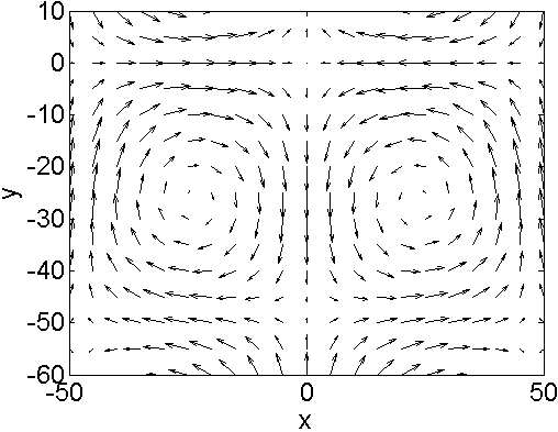
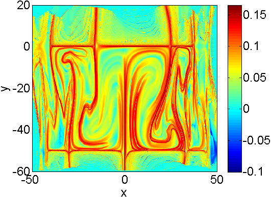
Abbildung 1: (a) Vector field and (b) FTLE field of the model given by (2) for two gyres with $A=10$, $\mu=0.005$, $\varepsilon=0.1$, $\psi=0$, $I=0.01$, and $s=50$. LCS are characterized by regions with maximum FTLE measures (denoted by red). In 2D flows, regions with maximum FTLE measures correspond to 1D curves.

Let ${\cal W}$ denote an obstacle-free workspace with flow dynamics given by (2). We assume a tessellation of ${\cal W}$ such that the boundaries of each cell roughly corresponds to the stable/unstable manifolds or LCS curves quantified by maximum FTLE ridges as shown in Fig. 2. In general, it may be unreasonable to expect small resource constrained autonomous vehicles to be able to track the LCS locations in real time. However, LCS boundary locations can be determined using historical data, ocean model data, e.g., data provided by the Navy Coastal Ocean Model (NCOM) databases, and/or data obtained a priori using LCS tracking strategies similar to (Hsieh et al., 2012). This information can then be used to obtain an LCS-based cell decomposition of ${\cal W}$. Fig. 2 shows two manual cell decompositions of the workspace where the cell boundaries roughly correspond to maximum FLTE ridges. In this work, we assume the tessellation of ${\cal W}$ is given and do not address the problem of automatic tessellation of the workspace to achieve a decomposition where cell boundaries correspond to LCS curves.

A tessellation of the workspace along boundaries characterized by maximum FTLE ridges makes sense since they separate regions within the flow field that exhibit distinct dynamic behavior and denote regions in the flow field where more escape events may occur probabilistically (Forgoston et al., 2011). In the time-independent case, these boundaries correspond to stable and unstable manifolds of saddle points in the system. The manifolds can also be characterized by maximum FTLE ridges where the FTLE is computed based on a backward (attracting structures) or forward (repelling structures) integration in time. Since the manifolds demarcate the basin boundaries separating the distinct dynamical regions, they are also regions that are uncertain with respect to velocity vectors within a neighborhood of the manifold. Therefore, switching between regions in neighborhoods of the manifold is influenced both by deterministic uncertainty as well as stochasticity due to external noise.

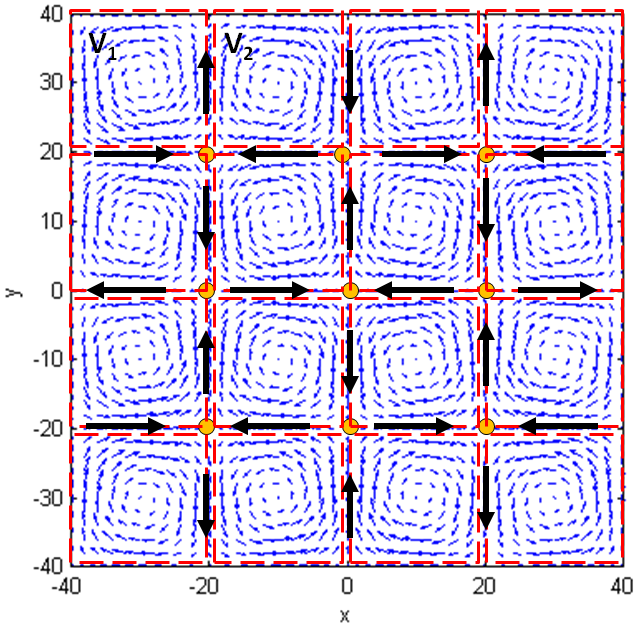
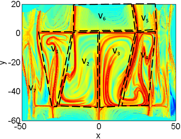
Abbildung 2: Two examples of LCS-based cell decomposition of the region of interest assuming a flow field given by (2). These cell decompositions were performed manually. (a) A $4\times 4$ time-independent grid of gyres with $A=0.5$, $\mu=0.005$, $\varepsilon=0$, $\psi=0$, $I=35$, and $s=20$. The stable and unstable manifolds of each saddle point in the system is shown by the black arrows. (b) An FTLE based cell decomposition for a time-dependent double-gyre system with the same parameters as Fig. 1.

Given an FTLE-based cell decomposition of ${\cal W}$, let ${\cal G}=({\cal V},{\cal E})$ denote an undirected graph whose vertex set ${\cal V}=\{V_{1},\ldots,V_{M}\}$ represents the collection of FTLE-derived cells in ${\cal W}$. An edge $e_{ij}$ exists in the set ${\cal E}$ if cells $V_{i}$ and $V_{j}$ share a physical boundary or are physically adjacent. In other words, ${\cal G}$ serves as a roadmap for ${\cal W}$. For the case shown in Fig. 2, adjacency of an interior cell is defined based on four neighborhoods. Let $N_{i}$ denote the number of AUVs or mobile sensing resources/robots within $V_{i}$. The objective is to synthesize agent-level control policies, or $\mathbf{u}_{k}$, to achieve and maintain a desired distribution of the $N$ agents across the $M$ regions, denoted by $\mathbf{\bar{N}}=[\bar{N}_{1},\ldots,\bar{N}_{M}]^{T}$, in an environment whose dynamics are given by (2).

We assume that robots are given a map of the environment, ${\cal G}$, and $\mathbf{\bar{N}}$. Since the tessellation of ${\cal W}$ is given, the LCS locations corresponding to the boundaries of each $V_{i}$ is also known a priori. Additionally, we assume robots co-located within the same $V_{i}$ have the ability to communicate with each other. This makes sense since coherent structures can act as transport barriers and prevent underwater acoustic wave propagation (Wang et al., 2009; Rypina et al., 2011). Finally, we assume individual robots have the ability to localize within the workspace, i.e., determine their own positions in the workspace. These assumptions are necessary to enable the development of a prioritization scheme within each $V_{i}$ based on an individual robot’s escape likelihoods in order to achieve the desired allocation. The prioritization scheme will allow robots to minimize the control effort expenditure as they move within the set ${\cal V}$. We describe the methodology in the following section.

2 Methodology

We propose to leverage the environmental dynamics and the inherent environmental noise to synthesize energy-efficient control policies for a team of mobile sensing resources/robots to maintain the desired allocation in ${\cal W}$ at all times. We assume each robot has a map of the environment. In our case, this translates to providing the robots the locations of LCS boundaries that define each $V_{i}$ in ${\cal G}$. Since LCS curves separate ${\cal W}$ into regions with distinct flow dynamics, this becomes analogous to providing autonomous ground or aerial vehicles a map of the environment which is often obtained a priori. In a fluidic environment, the map consists of the locations of the maximum FTLE ridges computed from data and refined, potentially in real-time, using a strategy similar to the one found in (Hsieh et al., 2012). Thus, we assume each robot has a map of the environment and has the ability to determine the direction it is moving in within the global coordinate frame, i.e., the ability to localize.

2.1 Controller Synthesis

Consider a team of $N$ robots initially distributed across $M$ gyres/cells. Since the objective is to achieve a desired allocation of $\mathbf{\bar{N}}$ at all times, the proposed strategy will consist of two phases: an auction to determine which robots within each $V_{i}$ should be tasked to leave/stay and an actuation phase where robots execute the appropriate leave/stay controller.

2.1.1 Auction Phase

The purpose of the auction phase is to determine whether $N_{i}(t)>\bar{N}_{i}$ and to assign the appropriate actuation strategy for each robot within $V_{i}$. Let $Q_{i}$ denote an ordered set whose elements provide robot identities that are arranged from highest escape likelihoods to lowest escape likelihoods from $V_{i}$.

In general, to first order we assume a geometric measure whereby the escape likelihood of any particle within $V_{i}$ increases as it approaches the boundary of $V_{i}$, denoted as $\partial V_{i}$ (Forgoston et al., 2011). Given ${\cal W}$, with dynamics given by (2), consider the case when $\varepsilon=0$ and $I\neq 0$, i.e., the case when the fluid dynamics is time-independent in the presence of noise. The boundaries between each $V_{i}$ are given by the stable and unstable manifolds of the saddle points within ${\cal W}$ as shown in Fig. 2. While there exists a stable attractor in each $V_{i}$ when $I=0$, the presence of noise means that robots originating in $V_{i}$ have a non-zero probability of landing in a neighboring gyre $V_{j}$ where $e_{ij}\in{\cal E}$. Here, we assume that robots experience the same escape likelihoods in each gyre/cell and assume that $P_{k}(\neg i|i)$, the probability that a robot escapes from region $i$ to an adjacent region, can be estimated based on a robot’s proximity to a cell boundary with some assumption of the environmental noise profile (Forgoston et al., 2011).

Let $d(\mathbf{q}_{k},\partial V_{i})$ denote the distance between a robot $k$ located in $V_{i}$ and the boundary of $V_{i}$. We define the set $Q_{i}=\{k_{1},\ldots,k_{N_{i}}\}$ such that $d(q_{k_{1}},\partial V_{i})\leq d(q_{k_{2}},\partial V_{i})\leq\ldots\leq d(q_{N_{i}},\partial V_{i})$. The set $Q_{i}$ provides the prioritization scheme for tasking robots within $V_{i}$ to leave if $N_{i}(t)>\bar{N}_{i}$. The assumption is that robots with higher escape likelihoods are more likely to be “pushed” out of $V_{i}$ by the environment dynamics and will not have to exert as much control effort when moving to another cell, minimizing the overall control effort required by the team.

In general, a simple auction scheme can be used to determine $Q_{i}$ in a distributed fashion by the robots in $V_{i}$ (Dias et al., 2006). If $N_{i}(t)>\bar{N}_{i}$, then the first $N_{i}-\bar{N}_{i}$ elements of $Q_{i}$, denoted by $Q_{i_{L}}\subset Q_{i}$, are tasked to leave $V_{i}$. The number of robots in $V_{i}$ can be established in a distributed manner in a similar fashion. The auction can be executed periodically at some frequency $1/T_{a}$ where $T_{a}$ denotes the length of time between each auction and should be greater than the relaxation time of the AUV/ASV dynamics.

2.1.2 Actuation Phase

For the actuation phase, individual robots execute their assigned controllers depending on whether they were tasked to stay or leave during the auction phase. As such, the individual robot control strategy is a hybrid control policy consisting of three discrete states: a leave state, $U_{L}$, a stay state, $U_{S}$, which is further distinguished into $U_{S_{A}}$ and $U_{S_{P}}$. Robots who are tasked to leave will execute $U_{L}$ until they have left $V_{i}$ or until they have been once again tasked to stay. Robots who are tasked to stay will execute $U_{S_{P}}$ if $d(q_{k},\partial V_{i})>d_{min}$ and $U_{S_{A}}$ otherwise. In other words, if a robot’s distance to the cell boundary is below some minimum threshold distance $d_{min}$, then the robot will actuate and move itself away from $\partial V_{i}$. If a robot’s distance to $\partial V_{i}$ is above $d_{min}$, then the robot will execute no control actions. Robots will execute $U_{S_{A}}$ until they have reached a state where $d(q_{k},\partial V_{i})>d_{min}$ or until they are tasked to leave at a later assignment round. Similarly, robots will execute $U_{S_{P}}$ until either $d(q_{k},\partial V_{i})\leq d_{min}$ or they are tasked to leave. The hybrid robot control policy is given by

$$U_{L}(\mathbf{q}_{k}) =\bm{\omega}_{i}\times c\frac{F(\mathbf{q}_{k})}{\|F(\mathbf{q}_{k})\|},$$ (3a)

$$U_{S_{A}}(\mathbf{q}_{k}) =-\bm{\omega}_{i}\times c\frac{F(\mathbf{q}_{k})}{\|F(\mathbf{q}_{k})\|},$$ (3b)

$$U_{S_{P}}(\mathbf{q}_{k}) =0.$$ (3c)

Here, $\mathbf{\omega}_{i}=[0,\,0,\,1]^{T}$ denotes counterclockwise rotation with respect to the centroid of $V_{i}$, with clockwise rotation being denoted by the negative and $c$ is a constant that sets the linear speed of the robots. The hybrid control policy generates a control input perpendicular to the velocity of the fluid as measured by robot $k$ and pushes the robot towards $\partial V_{i}$ if $U_{L}$ is selected, away from $\partial V_{i}$ if $U_{S_{A}}$ is selected, or results in no control input if $U_{S_{P}}$ is selected The hybrid control policy is summarized by Algorithm 1 and Fig. 3.

Algorithm 1 Auction Phase

1:  if $ElapsedTime==T_{a}$ then

2:     Determine $N_{i}(t)$ and $Q_{i}$

3:     $\forall k\in Q_{i}$

4:     if $N_{i}(t)>\bar{N}_{i}$ then

5:        if $k\in Q_{L}$ then

6:           $u_{k}\leftarrow U_{L}$

7:        else

8:           $u_{k}\leftarrow U_{S}$

9:        end if

10:     else

11:        $u_{k}\leftarrow U_{S}$

12:     end if

13:  end if

In general, the Auction Phase is executed at a frequency of $1/T_{a}$ which means robots also switch between controller states at a frequency of $1/T_{a}$. To further reduce actuation efforts exerted by each robot, it is possible to limit a robot’s actuation time to a period of time $T_{c}\leq T_{a}$. Such a scheme may prolong the amount of time required for the team to achieve the desired allocation, but may result in significant energy-efficiency gains. We further analyze the proposed strategy in the following sections.

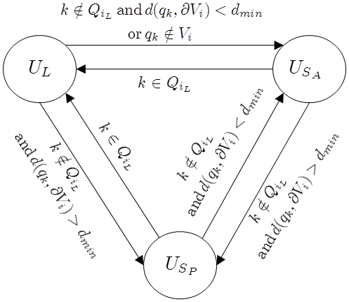
Abbildung 3: Schematic of the single-robot hybrid robot control policy.

3 Analysis

In this section, we discuss the theoretical feasibility of the proposed distributed allocation strategy. Instead of the traditional agent-based analysis, we employ a macroscopic analysis of the proposed distributed control strategy given by Algorithm 1 and (3). We first note that while the single robot controller shown in Fig. 3 results in an agent-level stochastic control policy, the ensemble dynamics of a team of $N$ robots each executing the same hybrid control strategy can be modeled using a polynomial stochastic hybrid system (pSHS). The advantage of this approach is that it allows the use of moment closure techniques to model the time evolution of the distribution of the team across the various cells. This, in turn, enables the analysis of the stability of the closed-loop ensemble dynamics. The technique was previously illustrated in (Mather and Hsieh, 2011). For completeness, we briefly summarize the approach here and refer the interested reader to (Mather and Hsieh, 2011) for further details.

The system state is given by $\mathbf{N}(t)=\left[N_{1}(t),\ldots,N_{M}(t)\right]^{T}$. As the team distributes across the $M$ regions, the rate in which robots leave a given $V_{i}$ can be modeled using constant transition rates. For every edge $e_{ij}\in{\cal E}$, we assign a constant $a_{ij}>0$ such that $a_{ij}$ gives the transition probability per unit time for a robot from $V_{i}$ to land in $V_{j}$. Different from Mather and Hsieh (2011), the $a_{ij}$s are a function of the parameters $c$, $T_{c}$, and $T_{a}$ of the individual robot control policy (3), the dynamics of the surrounding fluid, and the inherent noise in the environment. Furthermore, $a_{ij}$ is a macroscopic description of the system and thus a parameter of the ensemble dynamics rather than the agent-based system. As such, the macroscopic analysis is a description of the steady-state behavior of the system and becomes exact as $N$ approaches infinity.

Given ${\cal G}$ and the set of $a_{ij}$s, we model the ensemble dynamics as a set of transition rules of the form:

$$N_{i}\xrightarrow{a_{ij}}N_{j}\quad\textrm{$\forall$ $e_{ij}\in{\cal E}$}.$$ (4)

The above expression represents a stochastic transition rule with $a_{ij}$ as the per unit transition rate and $N_{i}(t)$ and $N_{j}(t)$ as discrete random variables. In the robotics setting, (4) implies that robots at $V_{i}$ will move to $V_{j}$ with a rate of $a_{ij}N_{i}$. We assume the ensemble dynamics is Markovian and note that in general $a_{ij}\neq a_{ji}$ and $a_{ij}$ encodes the inverse of the average time a robot spends in $V_{i}$.

Given (4) and employing the extended generator we can obtain the following description of the moment dynamics of the system:

$$\tfrac{d}{dt}\mathrm{E}[\mathbf{N}] =\mathbf{A}\mathrm{E}[\mathbf{N}]$$ (5)

where $[\mathbf{A}]_{ij}=a_{ji}$ and $[\mathbf{A}]_{ii}=-\sum_{(i,j)\in\cal{E}}a_{ij}$ (Mather and Hsieh, 2011). It is important to note that $\mathbf{A}$ is a Markov process matrix and thus is negative semidefinite. This, coupled with the conservation constraint $\sum_{i}N_{i}=N$ leads to exponential stability of the system given by (5) (Klavins, 2010).

In this work, we note that $a_{ij}$s can be determined experimentally after the selection of the various parameters in the distributed control strategy. While the $a_{ij}$s can be chosen to enable the team of robots to autonomously maintain the desired steady-state distribution (Hsieh et al., 2008), extraction of the control parameters from user specified transition rates is a direction for future work. Thus, using the technique described by Mather and Hsieh (2011), the following result can be stated for our current distributed control strategy

Theorem 1

Given a team of $N$ robots with kinematics given by (1) and $\mathbf{v}_{f}$ given by (2), the distributed allocation strategy given by Algorithm 1 and (3), at the ensemble level is stable and achieves the desired allocation strategy.

For the details of the model development and the proof, we refer the interested reader to (Mather and Hsieh, 2011).

4 Simulation Results

We validate the proposed control strategy described by Algorithm (1) and (3) using three different flow fields:

1. the time invariant wind driven multi-gyre model given by (2) with $\varepsilon=0$,

2. the time varying wind driven multi-gyre model given by (2) for a range of $\omega\neq 0$ and $\varepsilon\neq 0$ values, and

3. an experimentally generated flow field using different values of $T_{a}$ and $c$ in (3).

We refer to each of these as Cases 1, 2, and 3 respectively. Two metrics are used to compare the three cases. The first is the mean vehicle control effort to indicate the energy expenditure of each robot. The second is the population root mean square error (RMSE) of the resulting robot population distribution with respect to the desired population. The RMSE is used to show effectiveness of the control policy in achieving the desired distribution.

All cases assume a team of $N=500$ robots. The robots are randomly distributed across the set of M gyres in ${\cal W}$. For the theoretical models, the workspace ${\cal W}$ consists of a $4\times 4$ set of gyres, and each $V_{i}\in{\cal V}$ corresponds to a gyre as shown in Fig. 2. We considered three sets sets of desired distributions, namely a Ring formation, a Block formation, and an L-shaped formation as shown in Fig. 4. The experimental flow data had a set of $3\times 4$ regions. The inner two cells comprised ${\cal W}$, while the complement, ${\cal W}^{C}$ consisted of the remaining cells. This designation of cells helped to isolate the system from boundary effects, and allowed the robots to escape the center gyres in all directions. The desired pattern for this experimental data set was for all the agents to be contained within a single cell. Each of the three cases was simulated a minimum of five times and for a long enough period of time until steady-state was reached.

Abbildung 4: Three desired distributions of the team of $N=500$ mobile sensing resources/robots. (a) A Ring pattern formation, (b) a Block pattern formation, and (c) an L-shaped pattern formation. Each box represents a gyre and the number designates the desired number of robots contained within each gyre.

4.1 Case I: Time-Invariant Flows

For time-invariant flows, we assume $\varepsilon=0$, $A=0.5$, $s=20$, $\mu=0.005$, and $I=35$ in (2). For the ring pattern, we consider the case when the actuation was applied for $T_{c}=fT_{a}$ amount of time where $f=0.1,0.2,\ldots,1.0$, and $T_{a}=10$. For the Block and L-Shape patterns, we considered the cases when $T_{c}=0.5T_{a}$ and $T_{c}=T_{a}$. The final population distribution of the team for the case with no controls and the cases with controls for each of the patterns are shown in Fig. 5.

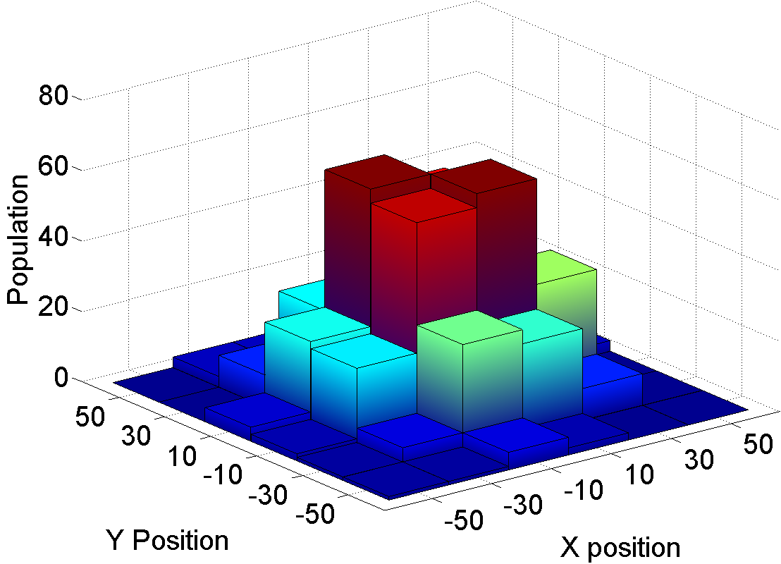
((a)) No Control

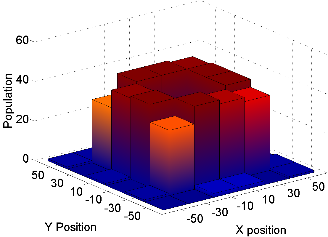
((b)) Ring

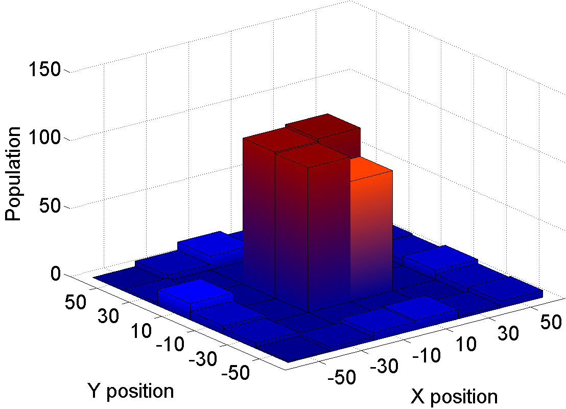
((c)) Block

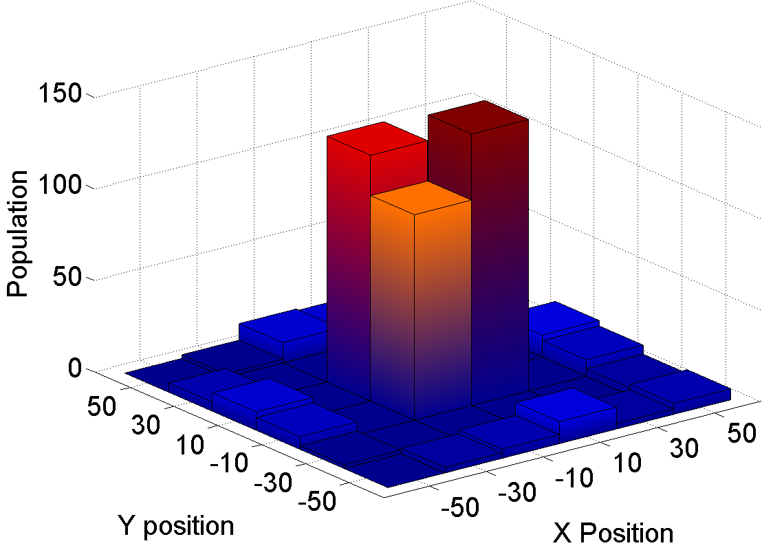
((d)) L-Shape

Abbildung 5: Histogram of the final allocations in the time-invariant flow field for the swarm of (a) passive robots exerting no controls and robots exerting control forming the (b) Ring pattern with $T_{c}=0.8T_{a}$ at $t=450$, (c) Block pattern with $T_{c}=T_{a}$ at $t=450$, and (d) L-shape pattern with $T_{c}=0.5T_{a}$ at $t=450$.

We compared our results to a baseline deterministic allocation strategy where the desired allocation is pre-computed and individual robots follow fixed trajectories when navigating from one gyre to another. For this baseline case, robots travel in straight lines at fixed speeds using a simple PID trajectory follower and treat the surrounding fluid dynamics as an external disturbance source. The RMSE results for all patterns are summarized in Table 1 and Fig. 6. The cumulative control effort per agent is shown in Fig. 7. From Fig. 6, we see that our proposed control strategy performs comparable to the baseline case especially when $T_{c}=T_{a}=10$ $sec$. In fact, even when $T_{c}<T_{a}$, our proposed strategy achieves the desired distribution. The advantage of the proposed approach lies in the significant energy gains when compared to the baseline case, especially when $T_{c}<T_{a}$, as seen in Fig. 7. We omit the cumulative control effort plots for the other cases since they are similar to Fig. 7.

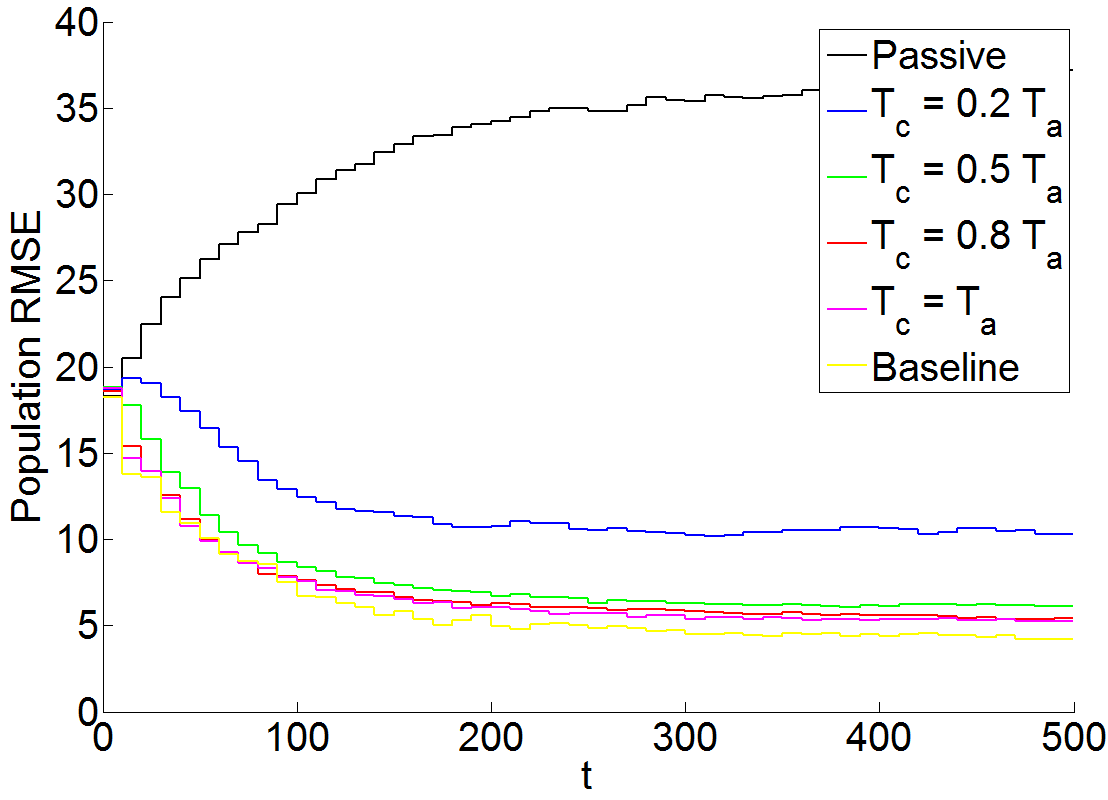
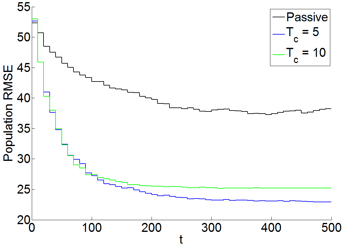
Abbildung 6: Comparison of the population RMSE in the time-varying flow for the (a) Ring formation, (b) the Block formation, and (c) the L-shape formation for different $T_{c}$, and for the PID control baseline controller in the Ring case with time-invariant flows.

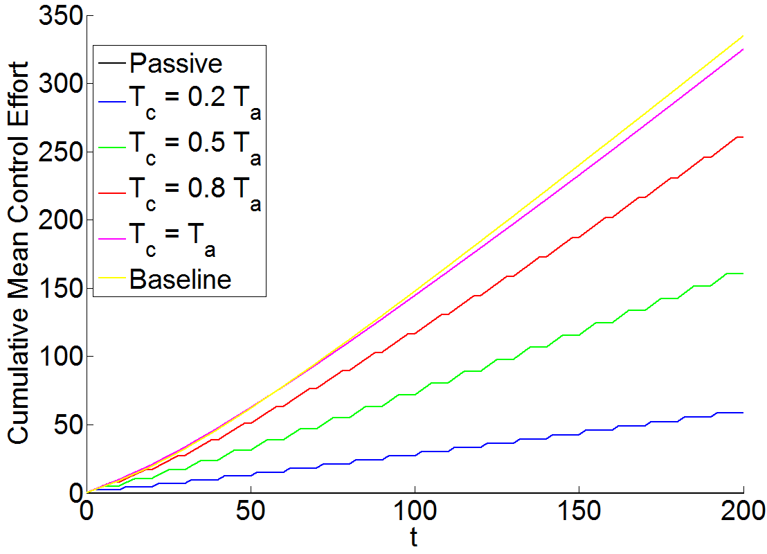
Abbildung 7: Comparison of the total control effort for the Ring pattern for different $T_{c}$ with the baseline controller for time-invariant flows.

In time-invariant flows, we note that for large enough $T_{c}$, our proposed distributed control strategy performs comparable to the baseline controller both in terms of steady-state error and convergence time. As $T_{c}$ decreases, less and less control effort is exerted and thus it becomes more and more difficult for the team to achieve the desired allocation. This is confirmed by both the RMSE results summarized in Table 1 and Fig. 6-6. Furthermore, while the proposed control strategy does not beat the baseline strategy as seen in Fig. 6, it does come extremely close to matching the baseline strategy performance. while requiring much less control effort as shown in Fig. 7 even at high duty cycles, i.e., when $T_{c}/T_{a}>0.5$.

More interestingly, we note that executing the proposed control strategy at 100% duty cycle, i.e., when $T_{c}=T_{a}$, in time-invariant flows did not always result in better performance. This is true for the cases when $T_{c}=0.5T_{a}=5$ for the Block and L-shaped patterns shown in Fig. 6 and 6. In these cases, less control effort yielded improved performance. However, further studies are required to determine the critical value of $T_{c}$ when less control yields better overall performance. In time-invariant flows, our proposed controller can more accurately match the desired pattern while using approximately $20\%$ less effort when compared to the baseline controller.

4.2 Case II: Time-Varying Flows

For the time-varying, periodic flow, we assume $A=0.5$, $s=20$, $\mu=0.005$, $I=35$, and $\psi=0$ in (2). Additionally, we considered the performance of our control strategy for different values of $\omega$ and $\varepsilon$ with $T_{a}=10$ and $T_{c}=8$ for the Ring formation and $T_{c}=5$ for the L-shaped formation. In all these simulations, we use the FTLE ridges obtained for the time-independent case to define the boundaries of each $V_{i}$. The final population distribution of the team for the case with no controls and the cases with controls for the Ring and L-shape patterns are shown in Fig. 8. The final population RMSE for the cases with different $\omega$ and $\varepsilon$ values for the Ring and L-shape patterns are shown in Fig. 9. These figures show the average of $10$ runs for each $\omega$ and $\varepsilon$ pair. In each of these runs, the swarm of mobile sensors were initially randomly distributed within the grid of $4\times 4$ cells. Finally, Fig. 10 shows the population RMSE as a function of time for the Ring and L-shape patterns respectively.

In time-varying, periodic flows we note that our proposed control strategy is able to achieve the desired final allocation even at 80% duty cycle, i.e., $T_{c}=0.8T_{a}$. This is supported by the results shown in Fig. 9. In particular, we note that the proposed control strategy performs quite well for a range of $\omega$ and $\varepsilon$ parameters for both the Ring and L-shape patterns. While the variation in final RMSE values for the Ring pattern is significantly lower than the L-shape pattern, the variations in final RMSE values for the L-shape are all within 10% of the total swarm population.

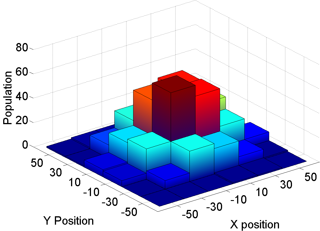
((a)) No Control

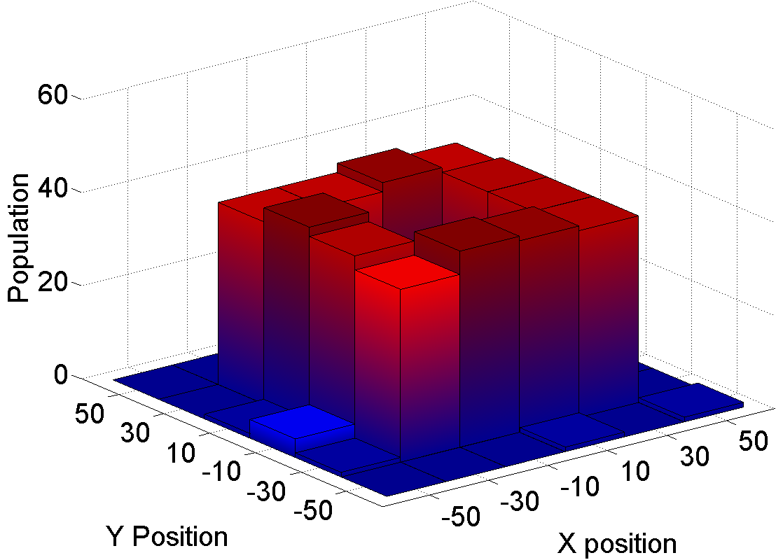
((b)) Ring

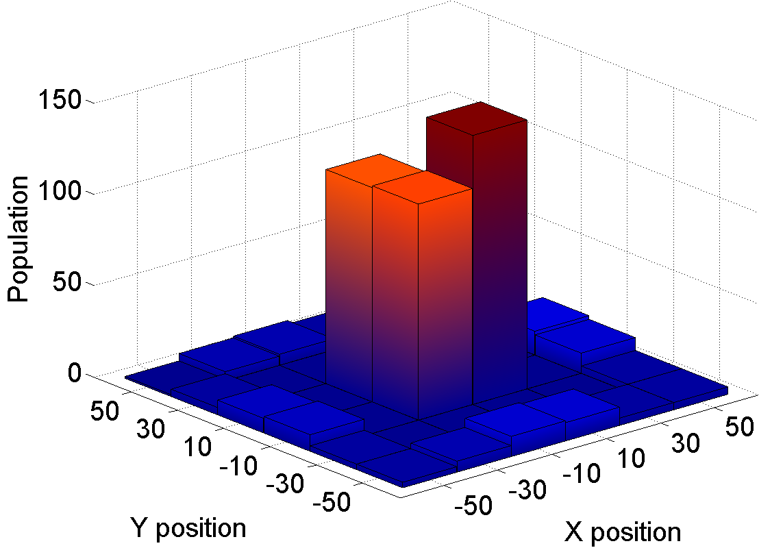
((c)) L-Shape

Abbildung 8: Histogram of the final allocations in periodic flows, with parameters of $\omega=\frac{5*\pi}{40}$ and $\varepsilon=5$, for the swarm of (a) passive robots exerting no controls and robots exerting control forming the (b) Ring pattern with $T_{c}=0.8T_{a}$ at $t=450$, and (c) L-Shape pattern with $T_{c}=0.5T_{a}$ at $t=450$.

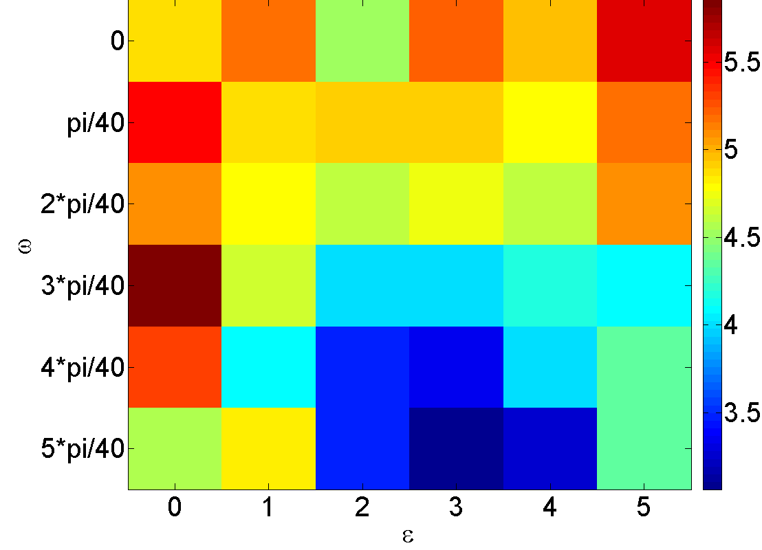
((a)) Ring

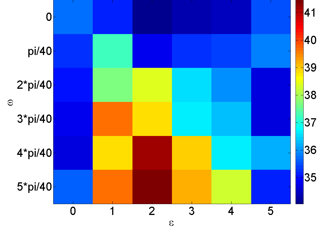
((b)) L-Shape

Abbildung 9: Final population RMSE for different values of $\omega$ and $\varepsilon$ for (a) the Ring formation and (b) the L-shaped formation.

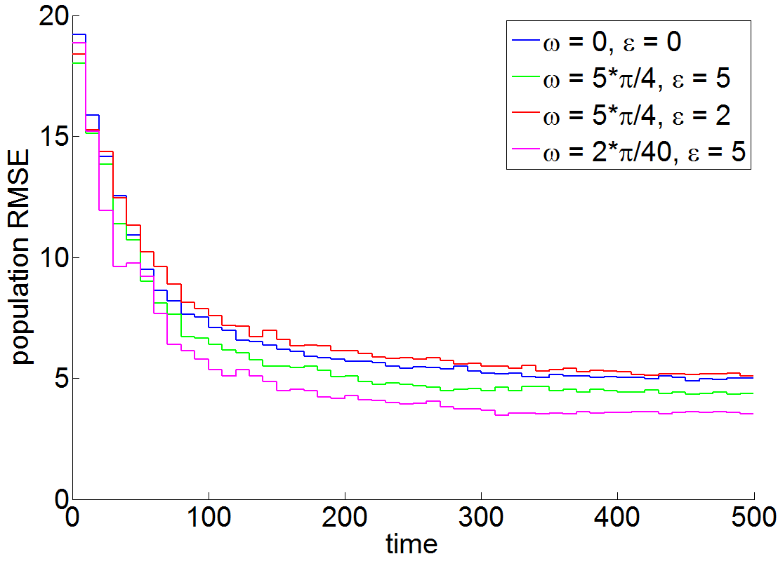
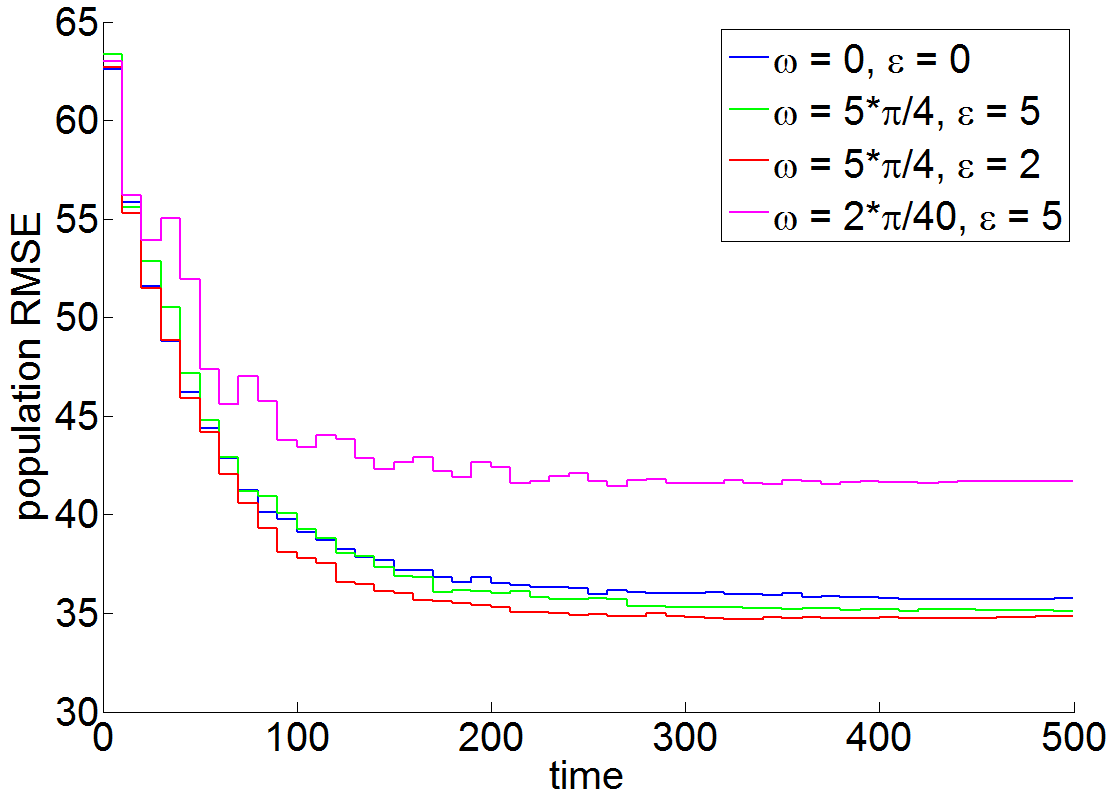
Abbildung 10: Comparison of RMSE over time for select $\omega$ and $\varepsilon$ pairs for the (a) Ring and (b) L-shaped patterns in periodic flows.

4.3 Case III: Experimental Flows

Using our $0.6m\times 0.6m\times 0.3m$ experimental flow tank equipped with a grid of $4x3$ set of driving cylinders, we generated a time-invariant multi-gyre flow field to use in simulation. Particle image velocimetry (PIV) was used to extract the surface flows at $7.5$ $Hz$ resulting in a $39\times 39$ grid of velocity measurements. The data was collected for a total of $60$ $sec$. Figure 11 shows the top view of our experimental testbed and the resulting flow field obtained via PIV. Further details regarding the experimental testbed can be found in (Michini et al., 2013). Using this data, we simulated a swarm of $500$ mobile sensors executing the control strategy given by (3).

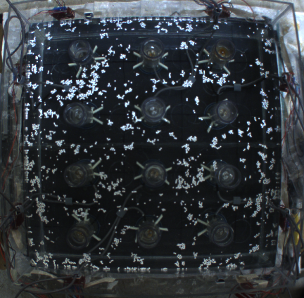
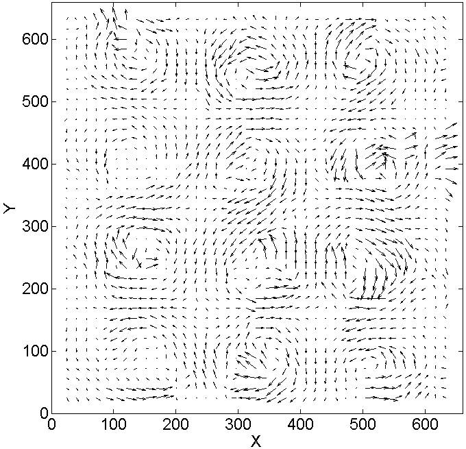
Abbildung 11: (a) Experimental setup of flow tank with $12$ driven cylinders. (b) Flow field for image (a) obtained via particle image velocimetry (PIV).

To determine the appropriate tessellation of the workspace, we used the LCS ridges obtained for the temporal mean of the velocity field. This resulted in the discretization of the space into a grid of $4\times 3$ cells. Each cell corresponds to a single gyre as shown Fig. 12. The cells of primary concern are the central pair and the remainder boundary cells were not used to avoid boundary effects and to allow robots to escape the center gyres in all directions. The robots were initially uniformly distributed across the two center cells and all $500$ robots were tasked to stay within the upper center cell. When no control effort is exerted by the robots, the final population distribution achieved by the team is shown in Fig. 13. With controls, the final population distribution is shown in Fig. 13. The control strategy was applied assuming $T_{c}/T_{a}=0.8$. The final RMSE for different values of $c$ in (3) and $T_{a}$ is shown in Fig. 14 and RMSE as a function of time for different values of $c$ and $T_{a}$ are shown in Fig. 14.

The results obtained using the experimental flow field shows that the proposed control strategy has the potential to be effective in realistic flows. However, the resulting performance will require good matching between the amount of control effort a vehicle can realistically exert, the frequency in which the auctions occur within a cell, and the time scales of the environmental dynamics as shown in in Figs. 14 and 14. This is an area for future investigation.

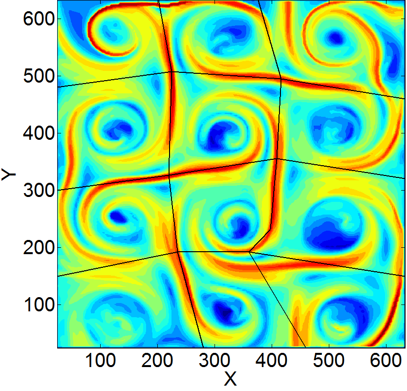
Abbildung 12: FTLE field for the temporal mean of the experimental velocity data. The field is discretized into a grid of $4\times 3$ cells whose boundaries are shown in black.

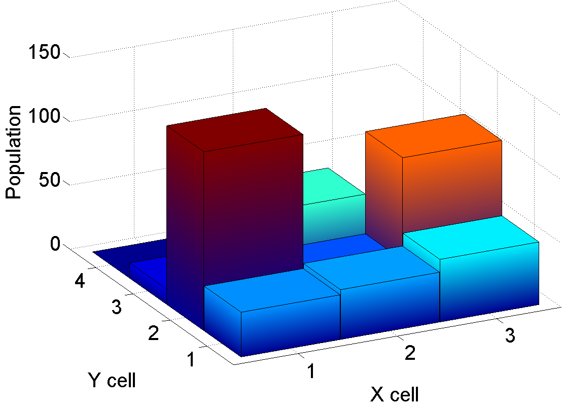
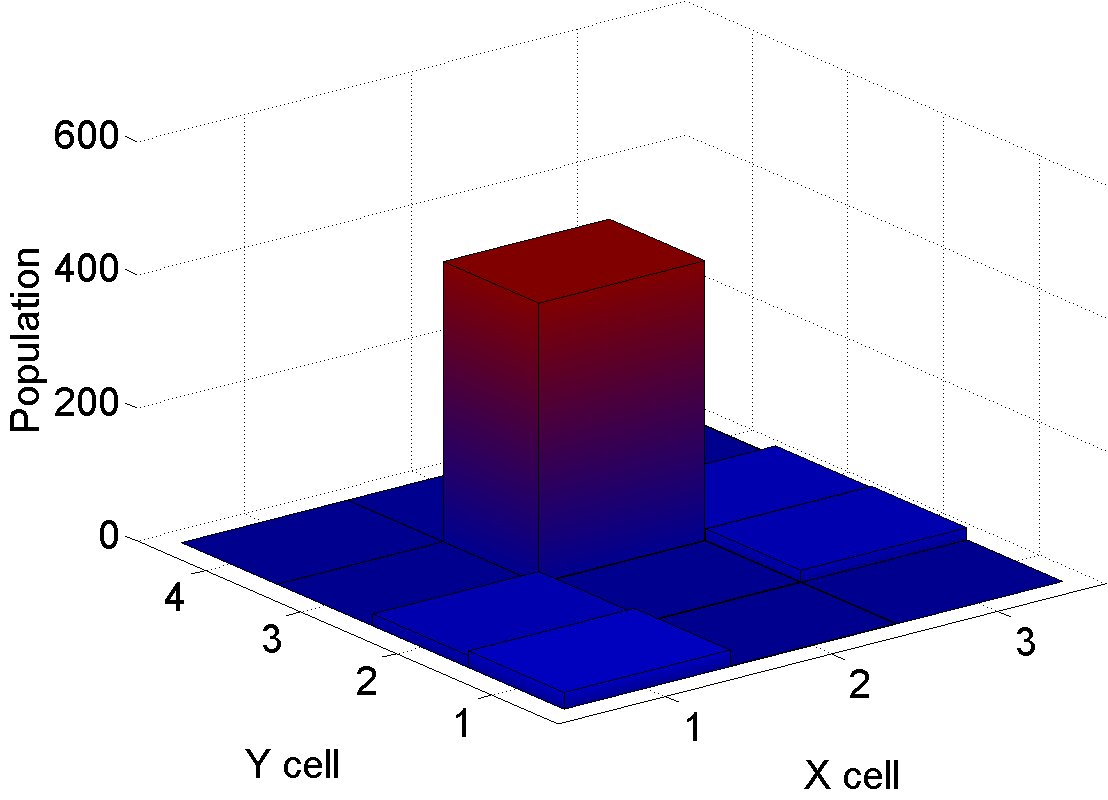
Abbildung 13: Population distribution for a swarm of $500$ mobile sensors over a period of $60$ $sec$ (a) with no controls, i.e., passive, and (b) with controls with $T_{c}=0.8T_{a}$.

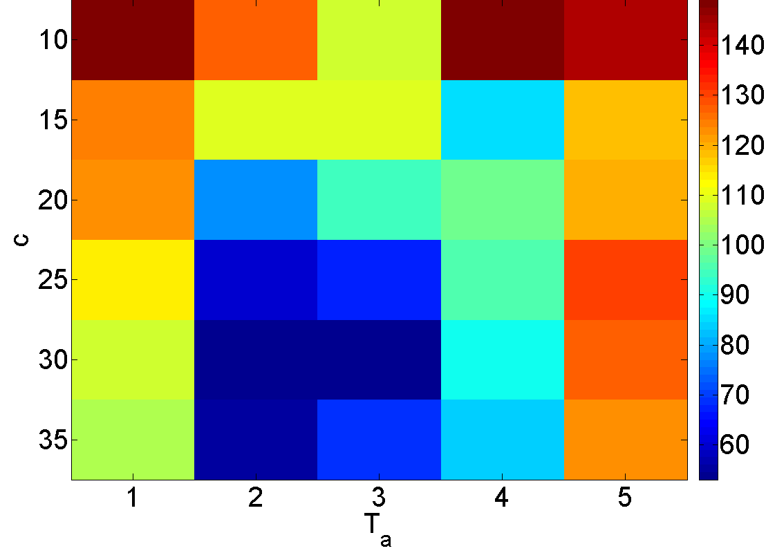
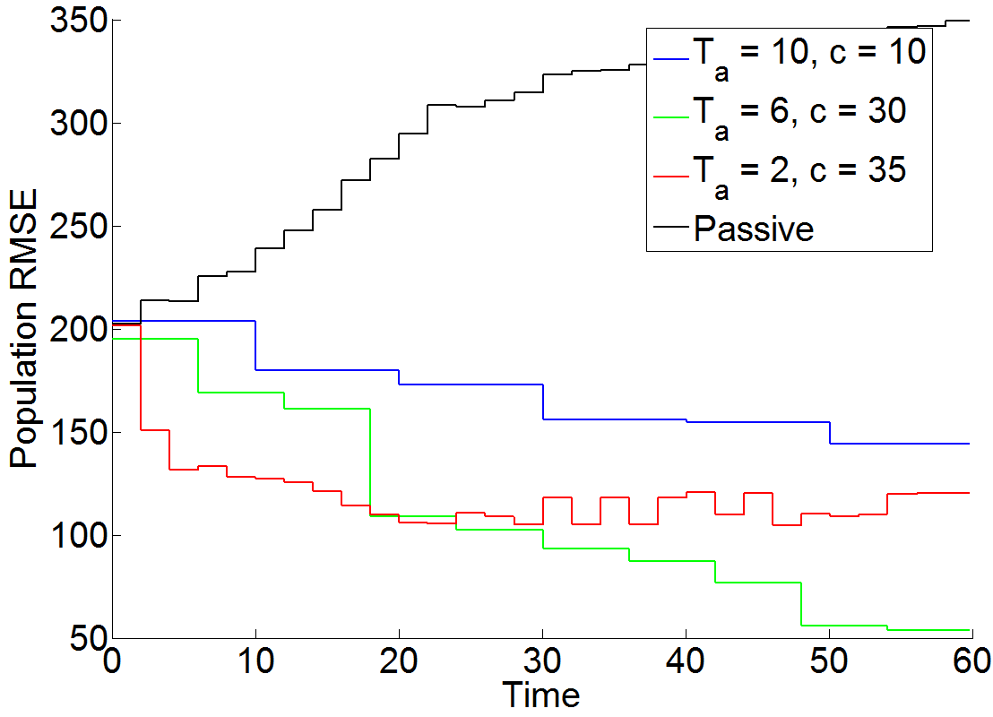
Abbildung 14: (a) Final RMSE for different values of $c$ and $T_{a}$ using the experimental flow field. $T_{c}/T_{a}=0.8$ is kept constant throughout. (b) RMSE over time for select $c$ and $T_{a}$ parameters on an experimental flow field. The duty cycle $T_{c}/T_{a}=0.8$ is kept constant throughout.

5 Conclusions and Future Outlook

In this work, we presented the development of a distributed hybrid control strategy for a team of robots to maintain a desired spatial distribution in a stochastic geophysical fluid environment. We assumed robots have a map of the workspace which in the fluid setting is akin to having some estimate of the global fluid dynamics. This can be achieved by knowing the locations of the material lines within the flow field that separate regions with distinct dynamics. Using this knowledge, we leverage the surrounding fluid dynamics and inherent environmental noise to synthesize energy efficient control strategies to achieve a distributed allocation of the team to specific regions in the workspace. Our initial results show that using such a strategy can yield similar performance as deterministic approaches that do not explicitly account for the impact of the fluid dynamics while reducing the control effort required by the team.

For future work we are interested in using actual ocean flow data to further evaluate our distributed allocation strategy in the presence of jets and eddies (Rogerson et al., 1999; Miller et al., 2002; Kuznetsov et al., 2002; Mancho et al., 2008; Branicki et al., 2011; Mendoza and Mancho, 2012). We also are interested in using more complicated flow models including a bounded single-layer PDE ocean model (Forgoston et al., 2011), a multi-layer PDE ocean model (Wang et al., 2009; Lolla et al., 2012), and realistic 2D and 3D unbounded flow models provided by the Navy Coastal Ocean Model (NCOM) database. Particularly, we are interested in extending our strategy to non-periodic, time-varying flows. In addition, we are currently developing an experimental testbed capable of generating complex 2D flows in a controlled laboratory setting. The objective is to be able to evaluate the proposed control strategy using experimentally generated flow field data whose dynamics are similar to realistic ocean flows. Finally, since our proposed strategy requires robots to have some estimate of the global fluid dynamics, another immediate direction for future work is to determine how well one can estimate the fluid dynamics given knowledge of the locations of Lagrangian coherent structures (LCS) in the flow field.

$T_{c}$	2	5	8	9	10
Ring Pattern	12.99	5.98	3.45	3.49	3.66
Block Pattern	-	11.21	-	-	12.72
L Pattern	-	30.09	-	-	30.45

Tabelle 1: Summary of the RMSE for each simulation pattern at $t=450$ with the time-invariant flow field. The RMSE for the Baseline case is 4.09.