The impact of systematic uncertainties in $\displaystyle\bm{N}$-body simulations on the precision cosmology from galaxy clustering: A halo model approach

Abstract

Dark matter $\displaystyle N$-body simulations provide a powerful tool to model the clustering of galaxies and help interpret the results of galaxy redshift surveys. However, the galaxy properties predicted from $\displaystyle N$-body simulations are not necessarily representative of the observed galaxy populations; for example, theoretical uncertainties arise from the absence of baryons in $\displaystyle N$-body simulations. In this work, we assess how the uncertainties in $\displaystyle N$-body simulations impact the cosmological parameters inferred from galaxy redshift surveys. Applying the halo model framework, we find that the velocity bias of galaxies in modelling the redshift-space distortions is likely to be the predominant source of systematic bias. For a deep, wide survey like BigBOSS, current 10 per cent uncertainties in the velocity bias limit $\displaystyle k_{\rm max}$ to 0.14 $\displaystyle h\,{\rm Mpc^{-1}}$. In contrast, we find that the uncertainties related to the density profiles and the galaxy occupation statistics lead to relatively insignificant systematic biases. Therefore, the ability to calibrate the velocity bias accurately – from observations as well as simulations – will likely set the ultimate limit on the smallest length scale that can be used to infer cosmological information from galaxy clustering.

1 Introduction

The large-scale distribution of galaxies has been used to probe the structure and composition of the universe for over three decades. From the pioneering analyses of the Lick catalogue (Groth & Peebles, 1977) and the CfA Redshift Survey (Huchra et al., 1983; Geller & Huchra, 1989) revealing the cosmic web, the APM Galaxy Survey hinting the departure from the standard cold dark matter model (Maddox et al., 1990) to the subsequent 2dF Galaxy Redshift Survey (Colless et al., 2001), the Sloan Digital Sky Survey (SDSS; York et al., 2000) and the VIMOS-VLT Deep Survey (Le Fèvre et al., 2005), galaxy redshift surveys have revolutionized the view of the large-scale structure of the universe. Recently, the WiggleZ Dark Energy Survey (Drinkwater et al., 2010) and the SDSS-III Baryon Oscillation Spectroscopic Survey (BOSS; Schlegel et al. 2009) have measured the galaxy clustering to unprecedented precision and provided stringent constraints on the cosmological parameters.

One of the most important features in the galaxy clustering is the baryon acoustic oscillations (BAO), originating from the waves in the primordial electron–photon plasma before the recombination. The sound horizon at the end of recombination is manifested as a peak in the real-space two-point correlation function or as wiggles in the Fourier-space power spectrum. This characteristic scale of BAO is considered as a standard ruler of the different evolution stages of the universe, and as a dark energy probe with relatively well-controlled systematics (Blake & Glazebrook, 2003; Seo & Eisenstein, 2003). Indeed, since its discovery (Miller et al., 2001; Cole et al., 2005; Eisenstein et al., 2005), BAO has been providing ever improving constraints on cosmological parameters (e.g., Percival et al., 2010; Blake et al., 2011; Anderson et al., 2012).

Beyond the BAO feature, the full scale-dependence of the clustering of galaxies contains much more information and can be used to constrain cosmology (e.g., Tegmark et al., 2006; Reid et al., 2010; Tinker et al., 2012; Cacciato et al., 2013) and the halo occupation statistics (e.g., Abazajian et al., 2005; Tinker et al., 2005; van den Bosch et al., 2007; Zheng & Weinberg, 2007; Zehavi et al., 2011). From the perspective of power spectrum $\displaystyle P(k)$, the number of modes increases as $\displaystyle k^{3}$, and the information content increases dramatically as one goes to smaller scales. However, when one tries to draw information from high $\displaystyle k$, especially at low redshift, the density perturbations become non-linear and difficult to model (e.g., Smith et al., 2003; Heitmann et al., 2010; Jennings et al., 2011), which can introduce significant systematic errors in the recovered cosmological parameters (e.g., de la Torre & Guzzo, 2012; Smith et al., 2012).

The analysis of galaxy clustering often relies on $\displaystyle N$-body simulations and synthetic galaxy catalogues to model the non-linearity on small scales, as well as to estimate the cosmic and sample covariances. For example, the WiggleZ team has validated their model for the non-linear galaxy power spectrum using the GiggleZ Simulation (Parkinson et al., 2012), while synthetic galaxy catalogues based on the Large Suite of Dark Matter Simulations (LasDamas) have been used in the galaxy clustering analysis of SDSS (Chuang & Wang, 2012; Xu et al., 2013).

For upcoming surveys, synthetic catalogues generated from $\displaystyle N$-body simulations will likely be routinely used to calibrate galaxy surveys. However, $\displaystyle N$-body simulations are not free from systematics. In $\displaystyle N$-body simulations, galaxies are assigned to haloes or dark matter particles based on models such as halo occupation distribution (HOD; Peacock & Smith, 2000; Scoccimarro et al., 2001; Berlind & Weinberg, 2002), abundance matching (Kravtsov et al., 2004; Vale & Ostriker, 2004), or semi-analytic models (White & Frenk, 1991; Kauffmann et al., 1993; Somerville & Primack, 1999; Cole et al., 2000). The galaxy populations predicted by simulations can be affected by intensive stripping in dense environment (e.g., Wetzel & White, 2010) and the absence of baryons (e.g., Weinberg et al., 2008; Simha et al., 2012). On the other hand, when one uses dark matter particles to model the behaviour of galaxies, systematic errors may arise because the positions and velocities of galaxies do not necessarily follow those of dark matter particles (Wu et al. 2013a). Hydrodynamical simulations that include proper treatments of baryonic physics can be another avenue to predict the properties of galaxies more reliably; however, because these simulations are more computationally intensive, it is not yet practical to use them to achieve the statistics and high resolution required by upcoming large surveys.

In addition, it has been shown that galaxies predicted from $\displaystyle N$-body simulations cannot recover the spatial distribution of observed galaxies. For example, Wu et al. (in preparation) have shown that in high-resolution $\displaystyle N$-body simulations of galaxy clusters, subhaloes tend to be prematurely destroyed and fail to predict the location of galaxies (also see Appendix A). The need to include “orphan galaxies” (galaxies not associated with subhaloes in simulations) to improve the completeness of predicted galaxies has been frequently addressed in the community (e.g., Gao et al., 2004; Wang et al., 2006; Guo et al., 2011); however, even including orphan galaxies does not lead to consistent galaxy clustering at all scales . For example, Guo et al. (2011) have shown that the galaxy population generated using the semi-analytic model applied to the Millennium Simulations overestimates the small scale clustering (also see Contreras et al. 2013).

In this paper, we examine the impact of the systematics in $\displaystyle N$-body simulations on the predictions of galaxy clustering. We calculate the galaxy power spectrum based on the halo model, with inputs from the results of recent $\displaystyle N$-body simulations. We use the information of the full power spectrum of galaxies to forecast the cosmological parameter constraints and determine at which scale these systematics start to become relevant. We specifically explore how these uncertainties will limit our ability to utilize the cosmological information from small scale.

This paper is organized as follows. In Section 2, we review the halo model prediction for galaxy power spectrum. In Section 3, we present our fiducial assumptions and discuss the information content associated with $\displaystyle P(k)$. Section 4 explores the self-calibration of HOD parameters. Section 5 addresses the impact of the uncertainties in the halo mass function on the cosmological constraints from galaxy clustering. Section 6 focuses on various systematics associated with the properties of galaxies in dark matter haloes in $\displaystyle N$-body simulations and presents the required control of these sources of systematic error. We conclude in Section 7. In Appendix A, we present the galaxy number density profile model used in this work. In Appendix B, we provide detailed derivation of the galaxy power spectrum based on the halo model. In Appendix C, we derive the power spectrum covariance.

2 Halo model and galaxy power spectrum: a review

Throughout this work, we use the power spectrum of galaxies $\displaystyle P(k)$ as our clustering statistic. Possible alternatives include the three-dimensional correlation function $\displaystyle\xi(r)$ and its two-dimensional analogue – the angular two-point function $\displaystyle w(\theta)$ or the projected two-point function $\displaystyle w_{p}(r_{p})$. While the Fourier-space power is more difficult to measure from the galaxy distribution, it is ‘closest to theory’ in the sense that the other aforementioned quantities are weighted integrals over $\displaystyle P(k)$. Therefore, it is easiest to see the effect of the uncertainties in theoretical modelling by using the power spectrum. While these different functions measured in a given galaxy survey contain the same information in principle, in data analysis sometimes discrepancies occur (e.g., Anderson et al., 2012).

2.1 Basic model

In this section, we provide the key equations of the galaxy power spectrum derived from the halo model, following Scherrer & Bertschinger (1991), Seljak (2000), and Cooray & Sheth (2002). The detailed derivation is provided in Appendix B.

The halo model assumes that all galaxies are inside dark matter haloes. To model the distribution of galaxies, we need the following distributions.

1. Statistics and spatial distribution of dark matter haloes:

   • Halo mass function, $\displaystyle{\rm d}n/{\rm d}M$, the number density of haloes as a function of the halo mass.

   • Halo bias, $\displaystyle b^{2}(M)=P_{\rm hh}(k)/P_{\rm lin}(k)$, where $\displaystyle P_{\rm hh}$ is the power spectrum of haloes and $\displaystyle P_{\rm lin}$ is the linear matter power spectrum. We limit our use of $\displaystyle b(M)$ to large scales where $\displaystyle b(M)$ is scale independent.

2. Statistics and spatial distribution of galaxies in a halo:

   • HOD function, $\displaystyle P(N|M)$, the probability distribution function of the number of galaxies in a halo of a given mass. The number of galaxies $\displaystyle N$ is further split into the contribution from central galaxies $\displaystyle N_{\rm cen}$ (0 or 1) and from satellite galaxies $\displaystyle N_{\rm sat}$.

   • Galaxy number density profile, $\displaystyle u(r|M)$, the radial dependence of the galaxy number density inside a halo of a given mass. We normalize $\displaystyle u$ such that $\displaystyle\int u(r|M){\rm d}^{3}{\bm{r}}=1$. We also use the density profile in Fourier space, $\displaystyle{\tilde{u}}({\bm{k}}|M)=\int{\rm d}^{3}{\bm{x}}u({\bm{x}}|M){\rm e}^{-i{\bm{k}}\cdot{\bm{x}}}\ ,$ and $\displaystyle{\tilde{u}}\rightarrow 1$ for small $\displaystyle k$.

The mean galaxy number density is given by

$${{{\bar{n}}_{\rm gal}}}\equiv\left\langle{{n_{\rm gal}}}\right\rangle=\int dM\frac{dn}{dM}\left\langle{N|M}\right\rangle\ .$$ (1)

The power spectrum is contributed by two galaxies in two different haloes (the two-halo term, $\displaystyle P_{\rm gg}^{\rm 2h}$) and two galaxies in the same halo (the one-halo term, $\displaystyle P_{\rm gg}^{\rm 1h}$):

$$\displaystyle P(k) \displaystyle= \displaystyle P_{\rm gg}^{\rm 1h}(k)+P_{\rm gg}^{\rm 2h}(k)$$ (2)

$$\displaystyle P_{\rm gg}^{\rm 2h}(k) \displaystyle= \displaystyle\left[\frac{1}{{{{\bar{n}}_{\rm gal}}}}\int dM\frac{dn}{dM}\left\langle{N|M}\right\rangle b(M){\tilde{u}}(k|M)\right]^{2}P_{\rm lin}(k)$$

$$\displaystyle P_{\rm gg}^{\rm 1h}(k) \displaystyle= \displaystyle\frac{1}{{{{\bar{n}}_{\rm gal}}}^{2}}\int dM\frac{dn}{dM}\left\langle{\displaystyle{\left.N\choose 2\right|}M}\right\rangle f(k|M)$$ (4)

Here $\displaystyle\left\langle{X|M}\right\rangle$ indicates the average value of quantity $\displaystyle X$ at a given halo mass $\displaystyle M$. In the one-halo term,

$$\left\langle{{\left.N\choose 2\right|}M}\right\rangle f(k|M) =\left[\left\langle{N_{\rm sat}|M}\right\rangle{\tilde{u}}(k|M)\right.$$

$$+\left.\frac{1}{2}\left\langle{N_{\rm sat}(N_{\rm sat}-1)|M}\right\rangle|{\tilde{u}}(k|M)|^{2}\right]\,,$$

which takes into account the contribution from central–satellite and satellite–satellite pairs (Berlind & Weinberg, 2002).

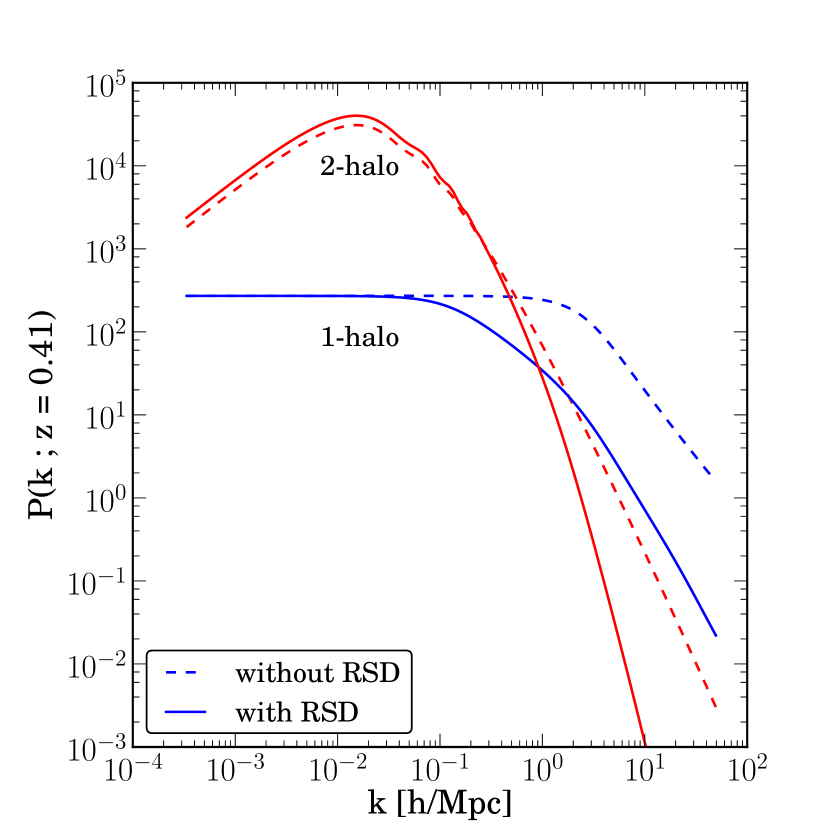
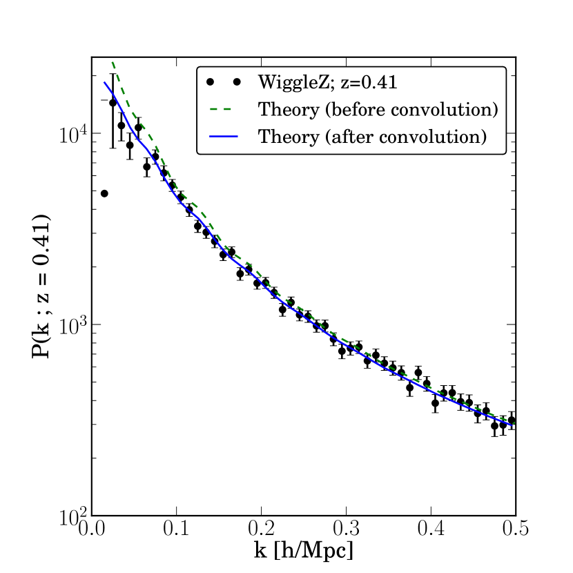
Figure 1: Galaxy power spectrum calculated based on the halo model. Left: the blue and red curves show the one- and two-halo terms, respectively. The solid curves include the RSD, while the dashed curves do not. RSD greatly reduce the power spectrum at small scale (the ‘Fingers-of-God’ effect), and only slightly shift the scale where one- and two-halo terms cross. Right: Our model fit to WiggleZ data from Parkinson et al. (2012). The blue solid curve shows the theoretical $\displaystyle P(k)$ with the best-fitting HOD parameters and has been convolved with the observational window function.

2.2 Redshift-space distortions

In observations, one cannot recover the exact three-dimensional spatial distribution of galaxies, because the redshifts of galaxies are impacted by their motions due to the local gravitational field and do not reflect their true distances. On larger scales, galaxies tend to move towards high-density regions along filaments, and these motions tend to squash the galaxy distribution along the line of sight and boost the clustering, a phenomenon known as the Kaiser effect (Kaiser, 1987). On small scales, the virial motions of galaxies inside a halo tend to make the galaxy distribution in the redshift space elongated along the line-of-sight, causing the so-called Fingers-of-God effect and reducing the small-scale power. In this section, we briefly describe the model we use for the redshift-space distortions (RSD) for $\displaystyle P(k)$, following Seljak (2001), White (2001), and Cooray & Sheth (2002). We adopt one of the simplified models – assuming the velocity distribution function to be Gaussian – and note that the improvement of the RSD model is currently an active research area.

Since the one-halo term involves the halo scale, we only consider the virial motions of galaxies inside a halo, which can be modelled as (Peacock, 1999)

$${\tilde{\delta}_{\rm gal}^{z}}({\bm{k}})={\tilde{\delta}_{\rm gal}}({\bm{k}}){\rm e}^{-\frac{1}{2}[k\sigma_{\rm v}(M)\mu]^{2}}\ ,$$ (5)

where $\displaystyle{\tilde{\delta}_{\rm gal}^{z}}$ and $\displaystyle{\tilde{\delta}_{\rm gal}}$ are the number density fluctuations of galaxies with and without the effect of RSD, $\displaystyle\sigma_{\rm v}(M)$ is the velocity dispersion of galaxies inside a halo of mass $\displaystyle M$ and $\displaystyle\mu=\hat{{\bm{k}}}\cdot\hat{{\bm{r}}}$. We average over $\displaystyle\mu$ to obtain the angular averaged one-halo term

$$P_{\rm gg}^{\rm 1h}(k)=\frac{1}{{{{\bar{n}}_{\rm gal}}}^{2}}\int dM\frac{dn}{dM}\left\langle{\displaystyle{\left.N\choose 2\right|}M}\right\rangle\,f_{R}(k|M)\ ,$$ (6)

where

$$\left\langle{{\left.N\choose 2\right|}M}\right\rangle f_{R}(k|M)=\left[\left\langle{N_{\rm sat}|M}\right\rangle{\tilde{u}}(k|M)R_{1}(M)\right.$$

$$+\left.\frac{1}{2}\left\langle{N_{\rm sat}(N_{\rm sat}-1)|M}\right\rangle|{\tilde{u}}(k|M)|^{2}R_{2}(M)\right]\ .$$

The factor

$$R_{p}(M)=\frac{\sqrt{{\rm{\rm\pi}}}}{2}\frac{{\rm erf}[k\sigma_{\rm v}(M)\sqrt{p/2}]}{k\sigma_{\rm v}(M)\sqrt{p/2}}$$ (7)

comes from averaging over $\displaystyle\mu$.

For the two-halo term, we multiply the large-scale and small-scale effects together (see Peacock 1999 and section 4 in Peacock & Dodds 1994)

$${\tilde{\delta}_{\rm gal}^{z}}({\bm{k}})=\left({\tilde{\delta}_{\rm gal}}({\bm{k}})+f(\Omega_{\rm M})\tilde{\delta}_{m}({\bm{k}})\mu^{2}\right){\rm e}^{-\frac{1}{2}[k\sigma_{\rm v}(M)\mu]^{2}}\ .$$ (8)

The first part is the familiar Kaiser result with $\displaystyle f(\Omega_{\rm M})\equiv d\ln D/d\ln a$, where $\displaystyle D(a)$ is the linear growth function of density fluctuations and $\displaystyle a$ is the scale factor. The density fluctuation of dark matter is denoted by $\displaystyle\tilde{\delta}_{m}$. The calculation thus includes not only the galaxy power spectrum, but also the matter power spectrum and the matter–galaxy cross power spectrum. After averaging over $\displaystyle\mu$, we obtain

$$P_{\rm gg}^{\rm 2h}(k)=\left(F_{g}^{2}+\frac{2}{3}F_{g}F_{v}+\frac{1}{5}F_{v}^{2}\right)P_{\rm lin}(k)\ ,$$ (9)

where

$$F_{g}(k)=\frac{1}{{{{\bar{n}}_{\rm gal}}}}\int dM\frac{dn}{dM}\left\langle{N|M}\right\rangle b(M)R_{1}(M){\tilde{u}(k|M)}$$ (10)

comes from the contribution of $\displaystyle{\tilde{\delta}_{\rm gal}}$, and

$$F_{v}(k)=f(\Omega_{\rm M})\frac{1}{\bar{\rho}}\int dM\frac{dn}{dM}Mb(M)R_{1}(M){\tilde{u}_{m}(k|M)}$$ (11)

comes from the contribution of $\displaystyle\tilde{\delta}_{m}$. Here $\displaystyle\tilde{u}_{m}(k|M)$ denotes the dark matter density profile normalized the same way as $\displaystyle{\tilde{u}}$, and $\displaystyle\bar{\rho}$ is the average matter density of the universe. We assume that $\displaystyle\tilde{u}_{m}(k|M)$ follows the Navarro–Frenk–White (NFW) profile (Navarro et al., 1997) throughout the paper.

The left-hand panel of Fig. 1 shows an example of the contribution to the total galaxy power spectrum by the one-halo (blue) and two-halo (red) terms. The input of halo model will be detailed in Section 3.1. The solid and dashed curves correspond to including and excluding the effect of RSD. As can be seen, including RSD significantly reduces the power at small scale. We also note that the scale where one- and two-halo terms cross shifts very slightly due to RSD.

The right-hand panel of Fig. 1 presents the comparison between our model and one of the power spectra from the WiggleZ survey, provided by Parkinson et al. (2012). The green dashed/blue solid curve corresponds to the theoretical $\displaystyle P(k)$ before/after convolving with the window function of WiggleZ. We assume that the HOD is described by the five parameters in equation (27); we fit for these five parameters and show the model corresponding to the best-fitting parameters. This figure is only for the purposes of illustration; details of the fitting procedure will be presented in a future paper.

3 Baseline model and fiducial dark energy constraints

In this section, we describe our inputs for the halo model, assumptions about the survey, predictions for the galaxy power spectrum, and Fisher matrix calculations of the statistical and systematic errors.

3.1 Baseline assumptions

We use the virial mass $\displaystyle M_{\rm vir}$ of dark matter haloes throughout this work and adopt the following functions in our halo model calculations:

• Mass function ($\displaystyle{\rm d}n/{\rm d}M$) and halo bias ($\displaystyle b(M,z)$): based on the fitting functions in Tinker et al. (2008); Tinker et al. (2010), which are derived from $\displaystyle N$-body simulations and can achieve approximately 5 per cent accuracy for the mass function and 6 per cent for the halo bias.

• Density profile: based on the universal NFW profile (Navarro et al., 1997), which is described by one concentration parameter $\displaystyle c_{\rm vir}$

  $$\displaystyle u_{\rm NFW}(r|M_{\rm vir}) \displaystyle\propto \displaystyle\frac{1}{(r/r_{s})(1+r/r_{s})^{2}}\ ,$$ (12)

  $$\displaystyle c_{\rm vir}(M_{\rm vir}) \displaystyle= \displaystyle R_{\rm vir}/r_{s}\ .$$

• Concentration–mass relation: based on the relation in Bhattacharya et al. (2013), which will be further discussed in Section 6.1. In the presence of significant scatter in the $\displaystyle c$–$\displaystyle M$ relation, we perform the integration

  $$u(r|M_{\rm vir})=\int dc_{\rm vir}P(c_{\rm vir}|M_{\rm vir})u(r|M_{\rm vir}(c_{\rm vir}))\ .$$ (13)

  Throughout this paper, we assume that $\displaystyle c_{\rm vir}$ has a Gaussian distribution for a given $\displaystyle M_{\rm vir}$ with a scatter of 0.33, based on the finding of Bhattacharya et al. (2013).

• Velocity dispersion: based on the scaling relation between dark matter velocity dispersion and halo mass from Evrard et al. (2008)

  $$\sigma_{\rm v}^{\rm DM}=1082.9\left(\frac{h(z)M_{200}}{10^{15}M_{\odot}}\right)^{0.3361}\ {\rm km\ s^{-1}}\ .$$ (14)

  We convert the mass $\displaystyle M_{200}$ to $\displaystyle M_{\rm vir}$ based on Hu & Kravtsov (2003). Since the scatter in the velocity dispersion is expected to be small (4 per cent), it is not included in our calculation.

• HOD: based on the parametrization from Zheng et al. (2005) and the fiducial parameters from Coupon et al. (2012), both of which will be discussed in detail in Section 4.

We assume a fiducial galaxy survey covering $\displaystyle f_{\rm sky}=1/3$ of the full sky (about 14 000 square degrees), similar to the BigBOSS experiment. We assume that the survey depth is comparable to the Canada–France–Hawaii Telescope Legacy Survey (CFHTLS) results presented in Coupon et al. (2012); specifically, we assume five redshift bins in the range $\displaystyle 0.2<z<1.2$, and the limiting magnitude in each bin is summarized in Table 1. We assume no uncertainties in the redshift measurements of galaxies. Given that the assumption of such a deep, wide spectroscopic survey may be somewhat optimistic, our required control of systematic errors may be somewhat more stringent than what BigBOSS needs.

We include seven cosmological parameters, whose fiducial values are based on the Wilkinson Microwave Anisotropy Probe 7 constraints (Komatsu et al., 2011): total matter density relative to critical $\displaystyle\Omega_{\rm M}=0.275$; dark energy equation of state today and its variation with scale factor $\displaystyle w_{0}=-1$ and $\displaystyle w_{a}=0$ respectively; physical baryon and matter densities $\displaystyle\Omega_{\rm b}h^{2}=0.02255$ and $\displaystyle\Omega_{\rm M}h^{2}=0.1352$; spectral index $\displaystyle n_{s}=0.968$; and the amplitude of primordial fluctuations $\displaystyle A=\Delta_{\zeta}^{2}(k=0.002h^{-1}\rm Mpc)=2.43\times 10^{-9}$. We assume a flat universe; thus, dark energy density $\displaystyle\Omega_{\rm DE}=1-\Omega_{\rm M}$.

3.2 Likelihood function of $\displaystyle P(k)$ and error forecasting

Here we follow the derivations in Scoccimarro et al. (1999) and Cooray & Hu (2001) but use a different convention for the Fourier transform (see Appendix B). If we assume a thin shell in $\displaystyle\ln k$ space with width $\displaystyle\delta\ln k$ around $\displaystyle\ln k_{i}$, the power spectrum estimator reads

$$\hat{P}(k_{i})=\int_{k_{i}}\frac{{\rm d}^{3}{\bm{k}}}{V_{s}(k_{i})}\delta({\bm{k}})\delta(-{\bm{k}})+\frac{1}{{{\bar{n}}_{\rm gal}}}\ ,$$ (15)

where

$$V_{s}(k_{i})=4{\rm\pi}k_{i}^{3}\delta\ln k\ ,$$ (16)

and $\displaystyle 1/{{\bar{n}}_{\rm gal}}$ accounts for the effect of shot noise. The first term of $\displaystyle\hat{P}$ is calculated based on the halo model results described in Section 2.2.

The covariance of power spectrum is given by

$$C_{ij} \equiv\left\langle{\hat{P}(k_{i})\hat{P}(k_{j})}\right\rangle-\left\langle{\hat{P}(k_{i})}\right\rangle\left\langle{\hat{P}(k_{j})}\right\rangle$$ (17)

$$\quad=\frac{(2{\rm\pi})^{3}}{V_{z}}\frac{2P(k_{i})^{2}}{V_{s}(k_{i})}\delta_{ij}+\bar{T}_{ij}\ ,$$

where the second term on the right-hand side is the contribution from the connected term given by the trispectrum describing the non-Gaussian nature of the random field

$$\bar{T}_{ij}=\int_{k_{i}}\frac{{\rm d}^{3}{\bm{k}}_{1}}{V_{s}(k_{i})}\int_{k_{j}}\frac{{\rm d}^{3}{\bm{k}}_{2}}{V_{s}(k_{j})}T({\bm{k}}_{1},-{\bm{k}}_{1},{\bm{k}}_{2},-{\bm{k}}_{2})\ .$$ (18)

We provide the detailed derivation in Appendix C. In equation (17) $\displaystyle V_{z}$ is the volume of the redshift bin, $\displaystyle V_{z}=\Omega_{\rm survey}\int r^{2}(z)/H(z)dz$, where the integral is performed over the redshift extent of the bin.

The calculation of $\displaystyle\bar{T}_{ij}$ involves four-point statistics, which is non-trivial to calculate. Fortunately, Cooray & Hu (2001) have shown that only the one-halo term dominates at the scale where the contribution of $\displaystyle\bar{T}_{ij}$ to $\displaystyle C_{ij}$ is not negligible; therefore, we only need to calculate the one-halo contribution:

$$T^{\rm 1h}(k_{1},k_{2},k_{3},k_{4}) =\frac{1}{V_{z}{{\bar{n}}_{\rm gal}}^{4}}\int dM\frac{dn}{dM}$$ (19)

$$\times\left\langle{{\left.N\choose 4\right|}M}\right\rangle f(k_{1},k_{2},k_{3},k_{4};M)$$

where

$$\left\langle{{\left.N\choose 4\right|}M}\right\rangle f(k_{1},k_{2},k_{3},k_{4};M)$$ (20)

$$=\left\langle{{\left.N_{\rm sat}\choose 3\right|}M}\right\rangle\frac{1}{4}\left({\rm\pi}_{i=1}^{3}\tilde{u}(k_{i}|M)+\mbox{cyc.}\right)$$

$$+\left\langle{{\left.N_{\rm sat}\choose 4\right|}M}\right\rangle{\rm\pi}_{i=1}^{4}\tilde{u}(k_{i}|M)\ .$$

Analogous to the case of $\displaystyle P_{\rm gg}^{\rm 1h}$ considered in Section 2.1, the first term accounts for quadruplets composed of one central and three satellite galaxies, and the second term accounts for the quadruplets composed of four satellite galaxies. We assume that $\displaystyle P(N_{\rm sat}|M)$ follows the Poisson distribution so that $\displaystyle\left\langle{\textstyle{N_{\rm sat}\choose 3}|M}\right\rangle=\left\langle{N_{\rm sat}|M}\right\rangle^{3}/3!$ and $\displaystyle\left\langle{\textstyle{N_{\rm sat}\choose 4}|M}\right\rangle=\left\langle{N_{\rm sat}|M}\right\rangle^{4}/4!$.

We employ the Fisher matrix formalism to forecast the statistical errors of the cosmological and nuisance parameters based on the fiducial survey. The Fisher matrix reads

$$F_{\alpha\beta}=\sum_{z}\sum_{i,j}\frac{\partial P_{i}}{\partial\theta_{\alpha}}\left[\frac{(2{\rm\pi})^{3}}{V_{z}}\frac{P_{i}^{2}}{2{\rm\pi}k_{i}^{3}\delta\ln k}\delta_{ij}+{T_{ij}}\right]^{-1}\!\!\frac{\partial P_{j}}{\partial\theta_{\beta}}$$

$$=\sum_{z}\sum_{i,j}\frac{\partial\ln P_{i}}{\partial\theta_{\alpha}}\left[\frac{(2{\rm\pi})^{3}}{V_{z}}\frac{1}{2{\rm\pi}k_{i}^{3}\delta\ln k}\delta_{ij}+\frac{T_{ij}}{P_{i}P_{j}}\right]^{-1}\!\!\frac{\partial\ln P_{j}}{\partial\theta_{\beta}}\ ,$$

where $\displaystyle\alpha$ and $\displaystyle\beta$ are indices of model parameters, while $\displaystyle i$ and $\displaystyle j$ refer to bins in wavenumber which have a constant logarithmic width $\displaystyle\delta\ln k$ and extend out to the maximum wavenumber $\displaystyle k_{\rm max}$. We adopt $\displaystyle\delta\ln k$ = 0.1, which has been tested to be small enough to ensure convergence. The best achievable error in the parameter $\displaystyle\theta_{\alpha}$ is given by

$$\sigma_{\theta_{\alpha}}=[({\mathsfbf F}^{-1})_{\alpha\alpha}]^{1/2}.$$ (21)

Throughout this work, unless otherwise indicated, the full set of parameters considered is given by

$$\theta_{\rm full} =(w_{0},w_{a},\Omega_{\rm DE},\Omega_{\rm M}h^{2},\Omega_{\rm b}h^{2},n_{s},\ln A;$$ (22)

$$\log_{10}M_{\rm min},\sigma_{\log_{10}M},\log_{10}M_{0},\log_{10}M_{1},\alpha_{\rm sat})\ .$$

The first seven are the cosmological parameters introduced in Section 3.1, while the last five are the nuisance parameters describing the HOD and will be discussed in Section 4.1.

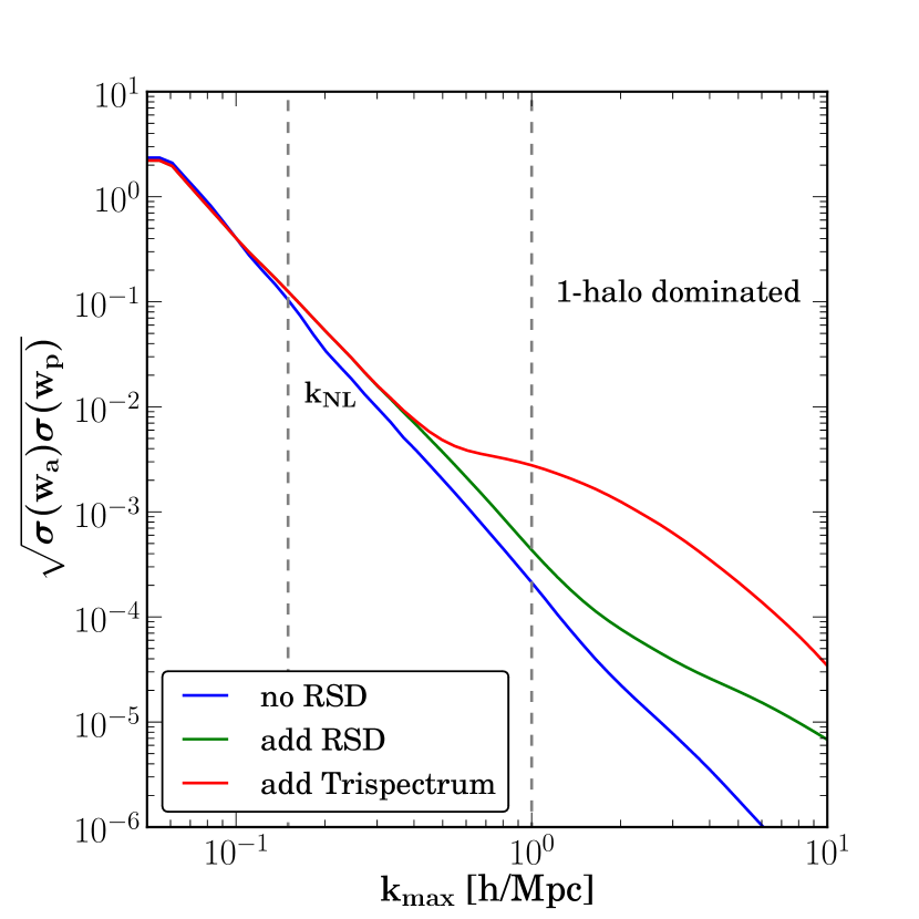
Figure 2: Dark energy information content from $\displaystyle P(k)$, based on our fiducial survey assumptions. The $\displaystyle x$-axis corresponds to the largest $\displaystyle k$ (smallest scale) assumed to be reliably measured and interpreted. The blue curve corresponds to a Gaussian likelihood function and assumes no RSD; it leads to unrealistically tight constraints for large $\displaystyle k_{\rm max}$. The green curve includes RSD, and the red curve further includes the trispectrum correction to the covariance matrix. As can be seen, including these two effects reduces the small-scale information.

3.3 Fiducial constraints without systematics

To represent the statistical power of an upcoming galaxy redshift survey, in the limiting case of no nuisance parameters, we consider the inverse of the square root of the dark energy figure of merit, originally defined as the inverse of the forecasted 95 per cent area of the ellipse in the $\displaystyle w_{0}$–$\displaystyle w_{a}$ plane (Huterer & Turner, 2001; Albrecht et al., 2006). In other words, our parameter of interest is $\displaystyle\sqrt{\sigma(w_{a})\sigma(w_{p})}$, where $\displaystyle w_{p}$ is the pivot that physically corresponds to $\displaystyle w(a)$ evaluated at the scale factor where the constraint is the best. This quantity takes into account the temporal variation of dark energy, and the square root serves to compare it fairly to the constant $\displaystyle w$; the two quantities, $\displaystyle\sigma(w)$ and $\displaystyle\sqrt{\sigma(w_{0})\sigma(w_{p})}$, tend to show very similar behaviour. For our fiducial survey, the statistical error in our parameter combination of interest is $\displaystyle\sqrt{\sigma(w_{a})\sigma(w_{p})}=$ 0.4 (or 0.003) for $\displaystyle k_{\rm max}=0.1$ (or 1) $\displaystyle h\,{\rm Mpc^{-1}}$, without external priors. When we add the Planck Fisher matrix (Hu, private communication), $\displaystyle\sqrt{\sigma(w_{a})\sigma(w_{p})}$ becomes 0.002 (or 0.0002) for $\displaystyle k_{\rm max}=0.1$ (or 1) $\displaystyle h\,{\rm Mpc^{-1}}$.

Fig. 2 presents the expected dark energy constraints as a function of $\displaystyle k_{\rm max}$, without nuisance parameters or systematic errors for the moment, for three levels of sophistication in the theory. We proceed in steps: the blue curve corresponds to no RSD (Section 2.1) with a Gaussian likelihood function. In this case, the dark energy constraints increase sharply with $\displaystyle k_{\rm max}$, indicating that these assumptions are unrealistic. The green curve includes the RSD (Section 2.2), which reduce the dark energy information from small scales. The red curve further includes the effect of non-Gaussian likelihood [$\displaystyle\bar{T}_{ij}$ from equation (18)], which reduces the information at high $\displaystyle k$ even more.

3.4 Systematic bias in model parameters

In this work, we estimate the systematic shifts in parameter inference caused by using an inadequate model. In particular, if we assume a problematic model that produces a power spectrum $\displaystyle P_{\rm sys}(k)$ that systematically deviates from the truth $\displaystyle P_{\rm fid}(k)$, we will obtain parameters that systematically deviate from their true values: $\displaystyle\theta_{\rm sys}=\theta_{\rm fid}+\Delta\theta$. The systematic shifts in parameters can be obtained through a modified Fisher matrix formalism (Knox et al., 1998):

$$\Delta\theta_{\alpha}=\sum_{\beta}({\mathsfbf F}^{-1})_{\alpha\beta}G_{\beta}\,,$$ (23)

where

$$G_{\beta} \equiv\sum_{z}\sum_{i,j}(\ln P_{\rm sys,\it i}-\ln P_{\rm fid,\it i})$$ (24)

$$\times\left[\frac{(2{\rm\pi})^{3}}{V_{z}}\frac{1}{2{\rm\pi}k_{i}^{3}\delta\ln k}\delta_{ij}+\frac{T_{ij}}{P_{i}P_{j}}\right]^{-1}\frac{\partial\ln P_{j}}{\partial\theta_{\beta}}\,.$$

To determine the significance of systematic errors, we calculate the systematic shifts $\displaystyle\Delta\chi_{\rm tot}^{2}$ in the full high-dimensional parameter space,

$$\Delta\chi^{2}_{\rm tot}=\Delta\theta^{T}{\mathsfbf F}\Delta\theta\,,$$ (25)

where $\displaystyle\Delta\theta$ is the vector of the systematic shifts of parameters. Both $\displaystyle\Delta\theta$ and the Fisher matrix $\displaystyle{\mathsfbf F}$ include cosmological and nuisance parameters. The systematic bias is considered significant if the inferred $\displaystyle\theta_{\rm sys}$ lies outside the 68.3 per cent confidence interval of the Gaussian likelihood function centred on $\displaystyle\theta_{\rm fid}$; in other words, the bias is ‘greater than the 1 $\displaystyle\sigma$ dispersion’. For example, in a full 12-dimensional parameter space considered here, the 68.3 per cent confidence interval corresponds to $\displaystyle\Delta\chi_{\rm tot}^{2}=13.7$.

4 Self-calibration of HOD parameters

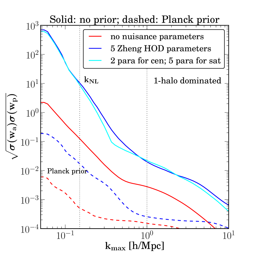
Figure 3: Self-calibration of HOD parameters. We show the dark energy constraints as a function of the highest $\displaystyle k$ used in the survey. The red curve corresponds to no nuisance parameters. The dark blue curve corresponds to five nuisance parameters based on the parametrization in Zheng et al. (2005), while the cyan curve corresponds to a piecewise continuous parametrization for satellite galaxies, with one parameter in each of the five mass bins. Including nuisance parameters in either parametrization systematically increases the dark energy uncertainties by one or two orders of magnitude. The dashed curves include the Planck prior and assume the same nuisance parameters as their solid-curve counterparts.

In this section, we focus on the efficacy of self-calibrating the HOD parameters, that is, determining these parameters from the survey concurrently with cosmological parameters. Since these HOD parameters are not known a priori, one usually marginalizes over them along with cosmological parameters (e.g., Tinker et al., 2012), which inevitably increases the uncertainties in cosmological parameters. Here we focus on the statistical uncertainties and assume no systematic error; in the next section, we will compare these statistical errors with systematic shifts of parameters.

We focus on two parametrizations of HOD: one is based on Zheng et al. (2005) and the other is based on a piecewise continuous parametrization.

4.1 Zheng et al.  parametrization

Redshift	$\displaystyle M_{g}-5\log_{10}h$	$\displaystyle\log_{10}{M_{\rm min}}$	$\displaystyle\log_{10}{M_{1}}$	$\displaystyle\log_{10}{M_{0}}$	$\displaystyle\sigma_{\log_{10}M}$	$\displaystyle{\alpha_{\rm sat}}$
$\displaystyle 0.2<z<0.4$	-17.8	11.18	12.53	7.54	0.40	1.10
$\displaystyle 0.4<z<0.6$	-18.8	11.48	12.66	10.96	0.43	1.09
$\displaystyle 0.6<z<0.8$	-19.8	11.77	12.83	11.54	0.50	1.07
$\displaystyle 0.8<z<1.0$	-20.8	12.14	13.21	12.23	0.35	1.12
$\displaystyle 1.0<z<1.2$	-21.8	12.62	13.79	8.67	0.30	1.50

Table 1: Fiducial values for the HOD parameters, adopted from Coupon et al. (2012) based on CFHTLS.

The HOD describes the probability distribution of having $\displaystyle N$ galaxies in a halo of mass $\displaystyle M$. In principle, the HOD is specified by the full distribution $\displaystyle P(N|M)$; in practice, modelling of the two-point statistics only requires $\displaystyle\left\langle{N_{\rm cen}|M}\right\rangle$, $\displaystyle\left\langle{N_{\rm sat}|M}\right\rangle$, and $\displaystyle\left\langle{N_{\rm sat}(N_{\rm sat}-1)|M}\right\rangle$. We follow the HOD parametrization from Zheng et al. (2005), which separates the contribution from central and satellite galaxies:

$$\displaystyle\left\langle{N_{\rm cen}|M}\right\rangle \displaystyle= \displaystyle\frac{1}{2}\left[1+{{\rm erf}}\left(\frac{\log_{10}M-\log_{10}M_{\rm min}}{\sigma_{\log_{10}M}}\right)\right]$$ (26)

$$\displaystyle\left\langle{N_{\rm sat}|M}\right\rangle \displaystyle= \displaystyle\left\langle{N_{\rm cen}|M}\right\rangle\times\left(\frac{M-M_{0}}{M_{1}}\right)^{\alpha_{\rm sat}}$$ (27)

The first equation describes the contribution from the central galaxy; $\displaystyle M_{\rm min}$ corresponds to the threshold mass where a halo can start to host a galaxy that is observable to the survey, and $\displaystyle\sigma_{\log_{10}M}$ describes the transition width of this threshold. The second equation describes the contribution from satellite galaxies, whose number is assumed to follow a power law, and $\displaystyle M_{0}$ is the cutoff mass. In addition, we make the widely-adopted assumption that $\displaystyle P(N_{\rm sat}|M)$ follows a Poisson distribution, i.e.,

$$\left\langle{N_{\rm sat}(N_{\rm sat}-1)|M}\right\rangle=\left\langle{N_{\rm sat}|M}\right\rangle^{2}\ .$$ (28)

We adopt the fiducial values from Coupon et al. (2012), which are constrained using the projected angular two-point correlation function $\displaystyle w(\theta)$ from the CFHTLS out to $\displaystyle z$ = 1.2. We use the same binning and limiting magnitude as in Coupon et al. (2012); the values are summarized in Table 1. We do not use the error bars quoted there as our priors because we would like all parameters to be self-calibrated consistently.

Under these assumptions, we have five nuisance parameters $\displaystyle(\log_{10}M_{\rm min},\ \sigma_{\log_{10}M},\ \log_{10}M_{0},\ \log_{10}M_{1},\ \alpha_{\rm sat})$ for each of the five redshift bins, i.e., 25 parameters in total. We assume that each of the five distinct nuisance parameters varies coherently across the five redshift bins, and is therefore described by a single parameter. Under this assumption, instead of 25 nuisance parameters, we only use five nuisance parameters to describe the uncertainties of all HOD parameters. We parametrize the variations around the fiducial values:

$$\theta^{\rm HOD}_{i}(z)=h_{i}\theta^{\rm HOD,fid}_{i}(z)\quad(i=1,...,5)\ ,$$ (29)

where $\displaystyle h_{i}$ are the dimensionless parameters describing the uncertainties of the aforementioned 5 HOD parameters. We note that this choice of five HOD parameters only represents one possible model; depending on the data available and the astrophysical motivation, in principle one can use a more general model to describe the evolution of HOD. Increasing the number of degrees of freedom describing the evolution of HOD will inevitably lead to degradation in the dark energy constraints, and it will be very important to establish the total number of degrees of freedom necessary to model the HOD and its uncertainties.

We explore how well these parameters can be self-calibrated by $\displaystyle P(k)$ without the aid of priors. Fig. 3 shows the dark energy constraints as a function of $\displaystyle k_{\rm max}$, with fixed nuisance parameters (red) and with these 5 marginalized nuisance parameters (dark blue). The RSD and the full covariances of $\displaystyle P(k)$ are included in this calculation. Clearly, the dark energy constraints are weakened by approximately about one or two orders of magnitude when we marginalize over HOD parameters.

4.2 Piecewise continuous parametrization of HOD parameters

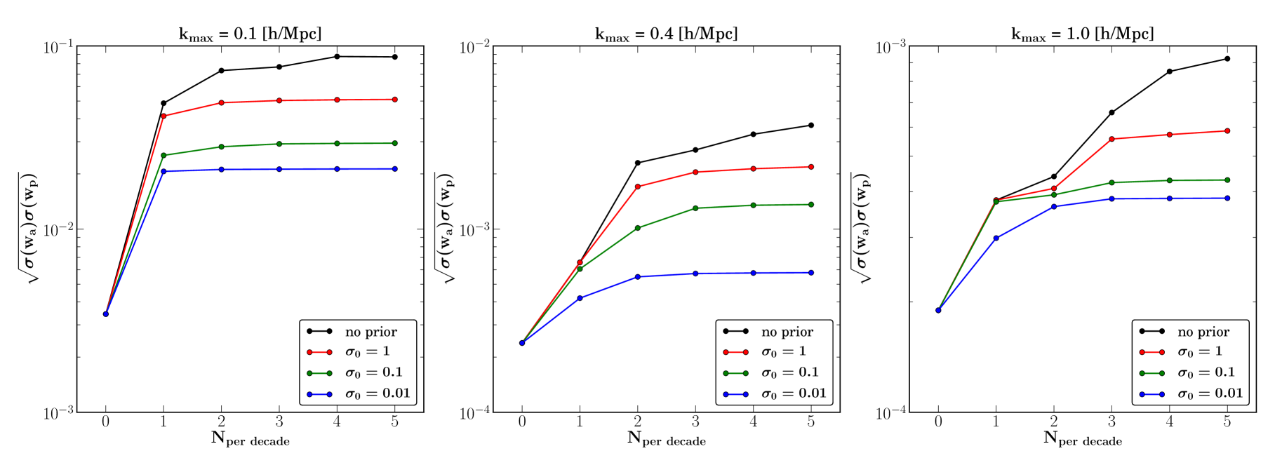
Figure 4: Dark energy constraints with self-calibrated piecewise continuous HODs. The three panels correspond to $\displaystyle k_{\rm max}$ = 0.1, 0.4 and 1 $\displaystyle h\,{\rm Mpc^{-1}}$. The $\displaystyle x$-axis corresponds to the number of parameters used to describe $\displaystyle\left\langle{N_{\rm sat}|M}\right\rangle$ per decade of mass, and the $\displaystyle y$-axis corresponds to the dark energy constraints. The black curve corresponds to no prior, and the constraints are degraded with larger number of parameters. The other curves correspond to consistently adding a fixed total prior per decade of mass; that is, $\displaystyle\sigma_{f_{i}}=\sigma_{0}\sqrt{N_{\rm per\ decade}}$ , where $\displaystyle\sigma_{0}$ = 1, 0.1, or 0.01. We note that one parameter per decade is sufficient for $\displaystyle k_{\rm max}$ = 0.1 $\displaystyle h\,{\rm Mpc^{-1}}$, while two or three parameters are needed for higher $\displaystyle k_{\rm max}$. Note that for higher $\displaystyle k_{\rm max}$, the HOD parameters are better self-calibrated, and the dark energy constraints are less dependent on the prior on HOD nuisance parameters.

One potential worry with the parametrization in equation (27) is whether $\displaystyle\left\langle{N_{\rm sat}|M}\right\rangle$ is accurately described by a power law. To address this, we propose a less model-dependent, piecewise continuous parametrization for $\displaystyle\left\langle{N_{\rm sat}|M}\right\rangle$. We divide the halo mass range into $\displaystyle n_{\rm bins}$ bins and assign a parameter describing the uncertainties of HOD in each bin. That is,

$$\left\langle{N_{\rm sat}|M}\right\rangle=\sum_{i=1}^{n_{\rm bins}}\Theta_{i}(M)f_{i}\left\langle{N_{\rm sat}|M}\right\rangle_{\rm fid}\ ,$$ (30)

where $\displaystyle\Theta_{i}(M)$ defines the binning and equals 1 in $\displaystyle[M_{i},M_{i+1}]$ and 0 elsewhere, while $\displaystyle f_{i}$ is the free parameter in bin $\displaystyle i$ and describes the uncertainty of $\displaystyle\left\langle{N_{\rm sat}|M}\right\rangle$ in this bin.

We still assume $\displaystyle P(N_{\rm sat}|M)$ to be a Poisson distribution, which now implies

$$\left\langle{N_{\rm sat}(N_{\rm sat}-1)|M}\right\rangle =\left\langle{N_{\rm sat}|M}\right\rangle^{2}$$ (31)

$$=\sum_{i=1}^{n_{\rm bins}}\Theta_{i}(M)f_{i}^{2}\left\langle{N_{\rm sat}|M}\right\rangle^{2}_{\rm fid}.$$

We start with one parameter per decade in mass, using $\displaystyle n_{\rm bins}=5$ parameters between $\displaystyle 10^{11}$ and $\displaystyle 10^{16}\,h^{-1}\rm M_{\odot}$, equally spaced in $\displaystyle\log_{10}M$. We assume these parameters to be independent of redshift. The cyan curve in Fig. 3 corresponds to marginalizing over these five piecewise continuous parameters for $\displaystyle\left\langle{N_{\rm sat}|M}\right\rangle$ and two parameters ($\displaystyle\log_{10}M_{\rm min}$, $\displaystyle\sigma_{\log_{10}M}$) for $\displaystyle\left\langle{N_{\rm cen}|M}\right\rangle$, with no prior on them.

Fig. 4 shows the dependence of dark energy constraints on the number of parameters describing $\displaystyle\left\langle{N_{\rm sat}|M}\right\rangle$ per decade of mass, $\displaystyle N_{\rm per\ decade}$. The three panels correspond to $\displaystyle k_{\rm max}$ = 0.1, 0.4, and 1 $\displaystyle h\,{\rm Mpc^{-1}}$. The Planck prior is included in this calculation. The black curve corresponds to no prior on $\displaystyle f_{i}$ and shows strong degradation with increasing $\displaystyle N_{\rm per\ decade}$ as one would expect. When $\displaystyle k_{\rm max}$ is small, the prior knowledge of HOD is important to improve the dark energy constraints. On the other hand, when $\displaystyle k_{\rm max}$ is large, HOD can be well self-calibrated, and the prior is not as important.

To enable a fair comparison of priors, however, we would like to increase the freedom in the HOD model while fixing the overall uncertainty per decade. To do this, we impose a fixed prior per decade of mass:

$$\sigma_{f_{i}}=\sigma_{0}\sqrt{N_{\rm per\ decade}}$$ (32)

so that the total prior per unit $\displaystyle\log_{10}M$, when we add the Fisher information from all $\displaystyle f_{i}$, is $\displaystyle\sigma_{0}$ regardless of the value of $\displaystyle N_{\rm per\ decade}$.

The red/green/blue curves in Fig. 4 correspond to imposing $\displaystyle\sigma_{0}=1/0.1/0.01$. For $\displaystyle k_{\rm max}=0.1\,h\,{\rm Mpc^{-1}}$, the dark energy constraints converge when we use one parameter per decade of mass regardless of the prior on nuisance parameters. When $\displaystyle k_{\rm max}>0.1\,h\,{\rm Mpc^{-1}}$, a few more parameters per decade in mass are required for the results to converge. For example, for $\displaystyle k_{\rm max}$ = 0.4 (1.0) $\displaystyle h\,{\rm Mpc^{-1}}$, we need two (three) parameters per decade to ensure convergence. The required number of parameters also somewhat depends on the prior.

We note that the HOD parameters are progressively better self-calibrated when we go to higher $\displaystyle k_{\rm max}$; when $\displaystyle k_{\rm max}=1\,h\,{\rm Mpc^{-1}}$, self-calibrating the five HOD parameters only moderately degrades the dark energy constraints. This finding encourages future surveys to further push towards high $\displaystyle k_{\rm max}$ for rich cosmological and astrophysical information.

5 Systematic errors due to the uncertainties in halo mass function

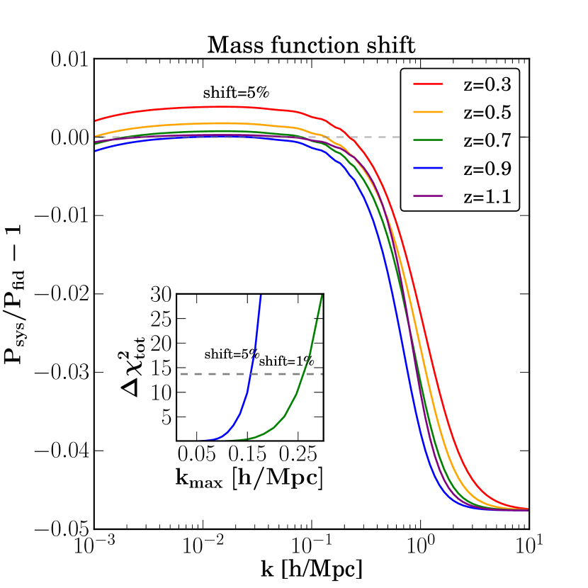
Figure 5: Impact of the uncertainty in the halo mass function on $\displaystyle P(k)$. The main panel shows the systematic shifts of $\displaystyle P(k)$ when the mass function is shifted by a constant 5 per cent (independent of mass and redshift). The inset shows $\displaystyle\Delta\chi^{2}_{\rm tot}$ as a function of $\displaystyle k_{\rm max}$ when the mass function is shifted by 1 or 5 per cent. The horizontal dashed line marks $\displaystyle\Delta\chi^{2}_{\rm tot}=13.7$, the 1-$\displaystyle\sigma$ deviation in the 12-dimensional parameter space. As can be seen, 5 per cent (1 per cent) allows $\displaystyle k_{\rm max}$ up to 0.15 (0.25) $\displaystyle h\,{\rm Mpc^{-1}}$.

In this section, we focus on the effect of the uncertainties in the halo mass function on the cosmological constraints from galaxy clustering. The mass function has been widely explored analytically (e.g., Press & Schechter, 1974) as well as numerically using dark matter $\displaystyle N$-body simulations (e.g., Sheth & Tormen, 1999; Sheth et al., 2001; Jenkins et al., 2001; Evrard et al., 2002; Reed et al., 2003; Warren et al., 2006; Lukić et al., 2007; Cohn & White, 2008; Tinker et al., 2008; Lukić et al., 2009; Crocce et al., 2010; Bhattacharya et al., 2013; Reed et al., 2013; Watson et al., 2013) and hydrodynamical simulations (e.g., Rudd et al., 2008; Stanek et al., 2010; Cui et al., 2012). The different fitting formulae for the mass function are often based on different halo identification methods and mass definitions; therefore, instead of drawing a direct comparison between different fitting formulae, we choose one specific fiducial model and explore the uncertainties relative to this model.

We use the fitting function from Tinker et al. (2008, described in Section 3.1), which has been calibrated based on a large suite of simulations implementing different $\displaystyle N$-body algorithms and different versions of $\displaystyle\Lambda$CDM cosmology; therefore, it is likely to fairly represent the uncertainties in the mass function calibration. Tinker et al. (2008) quoted a statistical uncertainty of $\displaystyle\lesssim 5$ per cent at $\displaystyle z=0$ ($\displaystyle\sim 1$ per cent around $\displaystyle M_{*}$). However, the uncertainties are presumably larger at higher redshift and can further increase if the effects of baryons are taken into account.

We explore the effect of a small constant shift of the halo mass function, parametrized as

$$\left(\frac{dn}{dM}\right)=(1+\epsilon)\left(\frac{dn}{dM}\right)_{\rm fid}\ .$$ (33)

The main panel of Fig. 5 shows the impact of $\displaystyle\epsilon=0.05$ on $\displaystyle P(k)$. For the two-halo term (small $\displaystyle k$), $\displaystyle P(k)$ changes by less than 1 per cent, because a constant shift in the mass function only affects $\displaystyle F_{v}$ describing the large-scale RSD (see equation 9). For the one-halo term (large $\displaystyle k$), $\displaystyle P(k)$ changes by $\displaystyle-5$ per cent, which can be easily seen from equation 6; the numerator includes one integration of $\displaystyle{\rm d}n/{\rm d}M$ (galaxy pairs in one halo) while the denominator includes the square of such an integration.

We next see how this systematic shift in $\displaystyle P(k)$ impacts cosmological parameters. We use $\displaystyle\Delta\chi^{2}_{\rm tot}=13.7$ [1 $\displaystyle\sigma$ errors in a 12-dimensional parameter space; see equation (25)] as our criterion of significant impact from the systematic error. We calculate $\displaystyle\Delta\chi^{2}_{\rm tot}$ using the Fisher matrix for seven cosmological parameters (Section 3.1) and five HOD parameters (Section 4.1). Throughout this and the next section, we use the Planck prior but no priors on HOD parameters. We believe that these two assumptions reflect reality in the next 5–10 years, when Planck data will firmly pin down certain combinations of cosmological parameters, while the determination of the nuisance HOD quantities will still be in flux. We note that unbiased priors always decrease the resulting systematic bias (for a proof, see appendix A of Bernstein & Huterer 2010) and make the theoretical requirements less stringent. Thus, any prior on HOD parameters will alleviate the systematic biases and make the required accuracy of theory less stringent.

The inset of Fig. 5 shows how $\displaystyle\Delta\chi^{2}$ depends on $\displaystyle k_{\rm max}$, for 5 per cent (blue) and 1 per cent (green) systematic shifts in the mass function. As can be seen, a 5 per cent (1 per cent) shift in the mass function can cause a significant systematic error at $\displaystyle k_{\rm max}=0.15$ (0.25) $\displaystyle h\,{\rm Mpc^{-1}}$. We note that at these scales, $\displaystyle P(k)$ is still dominated by the two-halo term; therefore, the systematic shifts caused by the mass function are mainly related to the large-scale redshift distortion (the Kaiser effect). However, this large-scale effect can be mitigated by prior knowledge of $\displaystyle\sigma_{8}$ (e.g., $\displaystyle\sigma_{8}$ constraints from galaxy cluster counts; Rozo et al. 2010), with which the large-scale galaxy bias can be calibrated. Therefore, by calibrating the large-scale clustering amplitude, one can in principle reduce the impact of the uncertainties in the mass function.

Finally, we note that the halo bias $\displaystyle b(M)$ is also currently being actively studied (e.g., Tinker et al., 2010; Ma et al., 2011; Manera & Gaztañaga, 2011; Paranjape et al., 2013). The uncertainty in the halo bias is related to the uncertainty in the mass function; for example, Tinker et al. (2010) have indicated that their fitting function for the halo bias has an $\displaystyle\sim 6$ per cent uncertainty, which is related to the uncertainty of their mass function. In addition, the uncertainties and systematics in $\displaystyle b(M)$ will lead to a constant shift in the two-halo term (see equation 9). In this case, holding the galaxy bias fixed will cause a huge systematic shift in cosmological parameters (for example, $\displaystyle\sigma_{8}$); therefore, it is necessary to fit the overall galaxy bias to the large-scale clustering data. In this work, we do not specifically explore the impact of uncertainties of the halo bias because the halo bias determines the large-scale clustering amplitude, which can be observationally calibrated when combined with independent knowledge of $\displaystyle\sigma_{8}$. On the other hand, we note that a scale-dependent bias can arise from the primordial non-Gaussianity (e.g., Dalal et al., 2008) or small-scale non-linearity (e.g., Smith et al., 2007). In this case, one could resort to multiple tracers of large-scale structure (e.g., Seljak, 2009; Cacciato et al., 2013), knowledge of primordial non-Gaussianity from the cosmic microwave background (e.g., Planck Collaboration, 2013) or higher order statistics (e.g., Marín et al., 2013) to better calibrate the scale dependence of the galaxy bias.

6 Systematic errors due to the uncertainties in halo properties

In this section, we explore the impact of four sources of theoretical uncertainties related to the properties of dark matter haloes coming from $\displaystyle N$-body simulations on the constraining power of $\displaystyle P(k)$. These sources of systematics are as follows:

• concentration–mass relation

• deviation of $\displaystyle{\tilde{u}}$ from the NFW profile

• deviation of $\displaystyle N_{\rm sat}$ from the Poisson distribution

• velocity bias

In particular, we address the following points.

• With the current level of uncertainties, what are the systematic errors in the prediction of $\displaystyle P(k)$? What are the biases in the parameter inference caused by these systematics?

• What is the smallest scale (largest $\displaystyle k_{\rm max}$) allowed by the current level of uncertainties?

• What is the required reduction of these uncertainties if we would like to push to higher $\displaystyle k_{\rm max}$?

We again use $\displaystyle\Delta\chi^{2}_{\rm tot}$ to assess the impact of systematic errors on the cosmological parameters, as described in the previous section. The summary of the impact of these systematics is presented in Fig. 6 and Table 2.

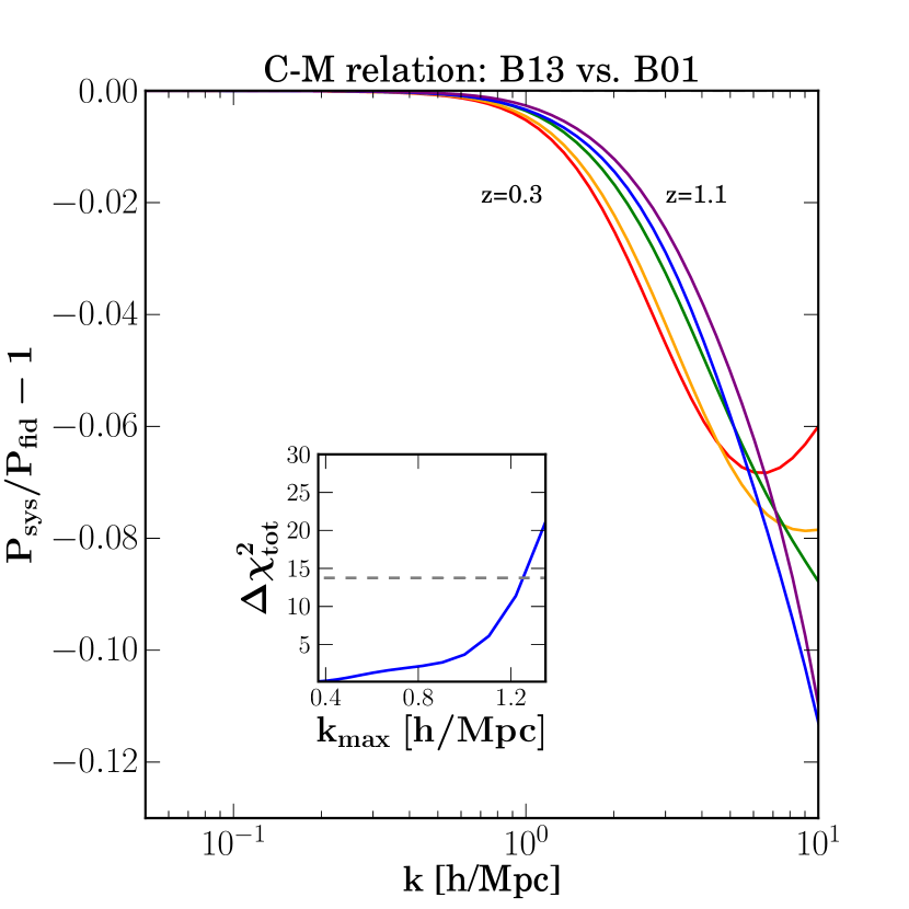
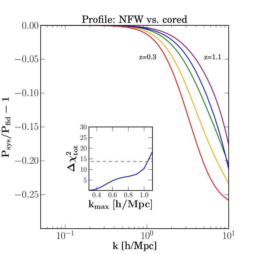
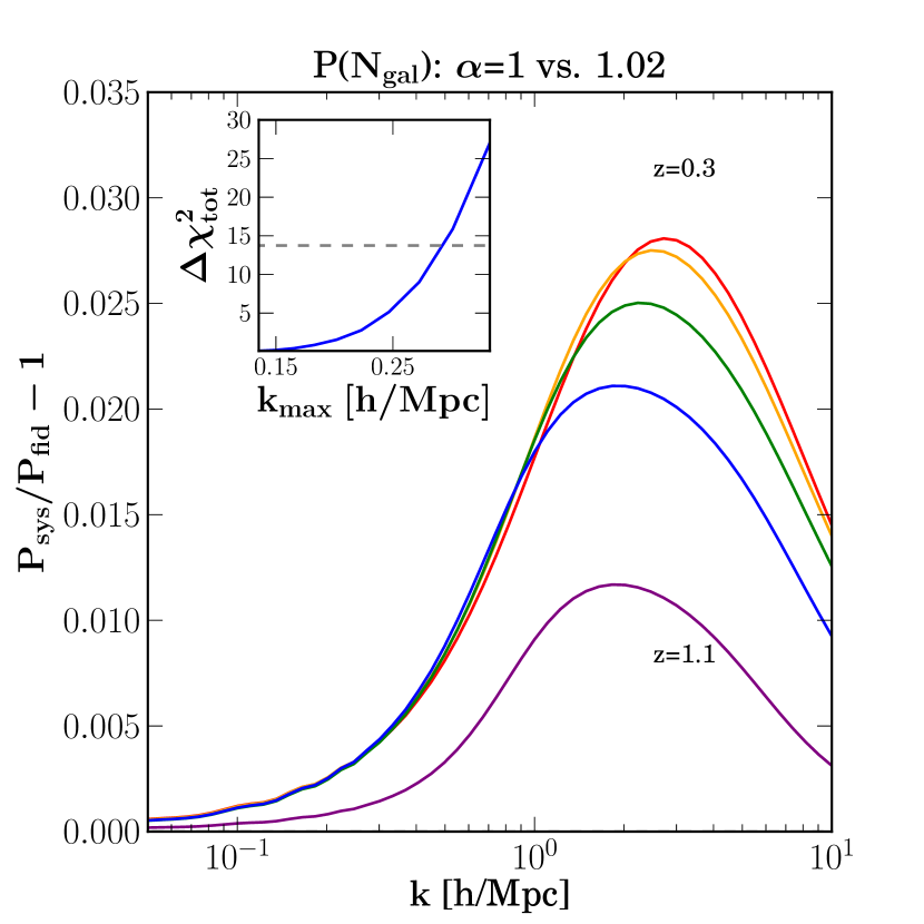
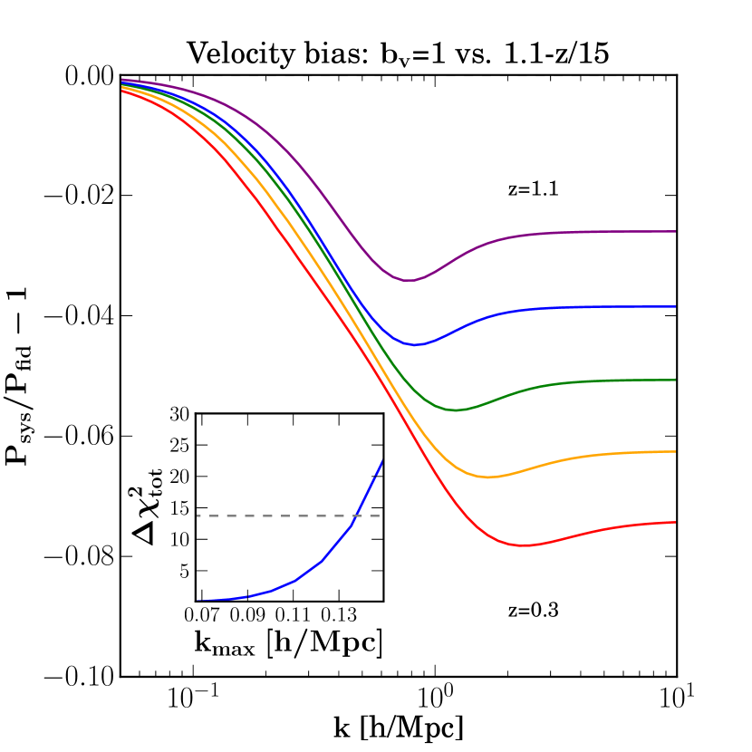
Figure 6: Systematic differences in $\displaystyle P(k)$ caused by the four sources of errors discussed in Section 6. In each panel, the main figure shows the fractional difference in $\displaystyle P(k)$ in the five redshift bins, while the inset shows the systematic error $\displaystyle\Delta\chi^{2}_{\rm tot}$ as a function of $\displaystyle k_{\rm max}$. The 1 $\displaystyle\sigma$ deviation in the 12-dimensional parameter space, $\displaystyle\Delta\chi^{2}_{\rm tot}=13.7$, is marked by the horizontal dashed line in each inset.

	Systematic	$\displaystyle k_{\rm max}$	$\displaystyle k_{\rm max}=0.3\,h\,{\rm Mpc^{-1}}$			$\displaystyle k_{\rm max}=1\,h\,{\rm Mpc^{-1}}$
	Difference	allowed	$\displaystyle\left\langle{\Delta P/P}\right\rangle$	Deviation $\displaystyle(\sigma)$	$\displaystyle f_{\rm sys}$ req.	$\displaystyle\left\langle{\Delta P/P}\right\rangle$	Deviation $\displaystyle(\sigma)$	$\displaystyle f_{\rm sys}$ req.
$\displaystyle c$–$\displaystyle M$ relation	B13 versus B01	1.3	0.00019	0	None	0.0039	0.014	None
Profile	NFW versus cored	1	0.0004	0	None	0.0074	0.56	None
P($\displaystyle N_{\rm sat}$)	$\displaystyle\rm\alpha$=1 versus 1.02	0.29	0.0037	1.3	0.93	0.016	15	0.23
Velocity bias	$\displaystyle\rm b_{v}$=1 versus 1.1-z/15	0.14	0.026	32	0.11	0.052	108	0.034

Table 2: Summary of the effects of the four sources of systematic error considered in Section 6. Note that $\displaystyle\left\langle{\Delta P/P}\right\rangle$ is calculated at $\displaystyle k=k_{\rm max}$ and averaged over the five redshift bins, and ‘$\displaystyle f_{\rm sys}$ req.’ is the required reduction factor in the amplitude of the systematic difference so that it becomes a 1 $\displaystyle\sigma$ effect in the full parameter space.

6.1 Concentration–mass relation

In the halo model, the one-halo term depends on the number density profile of galaxies, $\displaystyle{\tilde{u}}(k|M)$. We assume that the galaxy distribution follows the dark matter distribution, which is well described by an NFW profile. We then use the concentration–mass relation of dark matter haloes from the literature to compute $\displaystyle{\tilde{u}}(k|M)$.

The concentration–mass relation has been calibrated with dark matter $\displaystyle N$-body simulations (e.g., Bullock et al., 2001; Neto et al., 2007; Duffy et al., 2008; Macciò et al., 2008; Kwan et al., 2013; Prada et al., 2012; Bhattacharya et al., 2013) and hydrodynamical simulations (e.g., Lau et al., 2009; Duffy et al., 2010; Rasia et al., 2013). Several observational programmes are also working towards pinning down this relation (e.g., Coe et al., 2012; Oguri et al., 2012). However, 10–20 per cent of uncertainties in the concentration–mass relation remain, and the concentration–mass relation also varies with cosmology and the implementation of baryonic physics (see, e.g., the review in Bhattacharya et al. 2013).

We investigate the impact of uncertainties in the concentration–mass relation by comparing the models from Bullock et al. (2001, B01 hereafter) and the recent calibration from Bhattacharya et al. (2013, B13 hereafter). These two models represent two extreme cases of the concentration–mass relation; therefore, using these two extreme cases sets the upper limit of the systematic bias caused by the $\displaystyle c$–$\displaystyle M$ relation. We assume a scatter of 0.33 for the $\displaystyle c$–$\displaystyle M$ relation in both cases. Ignoring this scatter will lead to an approximately 0.5 per cent difference in $\displaystyle P(k)$ at $\displaystyle k\approx 1\,h\,{\rm Mpc^{-1}}$.

Our baseline model is from the recent formula given by B13 (based on virial overdensity):

$$\displaystyle c(\nu) \displaystyle= \displaystyle D(z)^{0.78}7.9\nu^{-0.28}$$ (34)

$$\displaystyle\nu \displaystyle= \displaystyle\frac{1}{D(z)}\left[1.12\left(\frac{M_{\rm vir}}{5\times 10^{13}h^{-1}\rm M_{\odot}}\right)^{0.3}+0.53\right].$$

We compare it with the model from B01:

$$c(M_{\rm vir})=\frac{9}{1+z}\left(\frac{M_{\rm vir}}{M_{*}(z)}\right)^{-0.13}.$$ (35)

These two calibrations agree near $\displaystyle M_{*}$ at $\displaystyle z=0$.

The top-left panel of Fig. 6 shows the relative change in the power spectrum $\displaystyle P(k)$, evaluated at five redshifts, due to the difference between B01 and B13. We find that $\displaystyle P(k)$ based on B01 is in general lower than that based on B13, because B01 predict lower concentrations at the high-mass end. Although B01 predict higher concentrations at the low-mass end, these haloes rarely contribute to the one-halo term and thus do not significantly boost clustering.

The inset in this panel shows the systematic shifts in the parameter space caused by different models, which are characterized by $\displaystyle\Delta\chi^{2}_{\rm tot}$. It can be seen that the systematic error starts to be comparable to the statistical error ($\displaystyle\Delta\chi^{2}_{\rm tot}=13.7$, marked by a horizontal dashed line) at $\displaystyle k_{\rm max}=1.2\ h\,{\rm Mpc^{-1}}$, which makes it a relatively unimportant source of systematic error.

We would now like to study the effects of improved calibration in the $\displaystyle c$–$\displaystyle M$ relation. A natural way to do this is to assume that the difference between the two extreme predictions has been reduced by some constant factor, and that the new value interpolates between the two original extremes. We define the interpolated value as

$$c_{\rm interp}(M)=c_{\rm fid}(M)+f_{\rm sys}\left(c_{\rm alt}(M)-c_{\rm fid}(M)\right)\ ,$$ (36)

where $\displaystyle c_{\rm fid}(M)$ and $\displaystyle c_{\rm alt}(M)$ are respectively the fiducial (say, B13) and the alternate (say, B01) models for the concentration–mass relation. Here $\displaystyle f_{\rm sys}$ is a tunable parameter that allows us to assess the effect of a fraction of the full systematics. The limiting cases are:

$$\displaystyle f_{\rm sys}=0 \displaystyle\quad\Longleftrightarrow\quad\mbox{no systematics}$$

$$\displaystyle f_{\rm sys}=1 \displaystyle\quad\Longleftrightarrow\quad\mbox{fiducial systematics \ .}$$

For a higher $\displaystyle k_{\rm max}$, the tolerance of systematics is smaller, and $\displaystyle f_{\rm sys}$ provides a measure for required reduction of systematics. For a given $\displaystyle k_{\rm max}$, we search for the appropriate $\displaystyle f_{\rm sys}$ value that makes the systematic negligible.

The blue curve in Fig. 7 shows the requirement on $\displaystyle f_{\rm sys}$ from the c-M relation as a function of $\displaystyle k_{\rm max}$. For all practical $\displaystyle k_{\rm max}$ values, $\displaystyle c$–$\displaystyle M$ does not require more precise calibrations from $\displaystyle N$-body simulations. The results are summarized in the ‘$\displaystyle c$–$\displaystyle M$ relation’ row of Table 2.

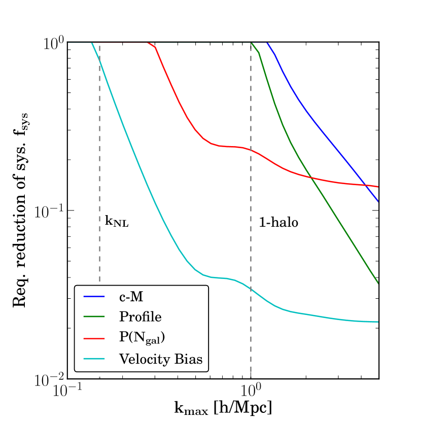
Figure 7: Required reduction of systematic errors, shown as the fraction of the current errors, for the four sources of systematic errors discussed in this paper, as a function of the maximum wavenumber considered in the survey. Note that the velocity bias requires the greatest improvement relative to the current knowledge.

6.2 Galaxy number density profile: deviation from NFW

Our fiducial model assumes that the galaxy distribution inside a halo is described by the NFW profile. However, $\displaystyle N$-body simulations have shown that the distribution of subhaloes in cluster-size haloes tends to be shallower than the NFW profile, and also shallower than the observed galaxy number density profile (e.g., Diemand et al., 2004; Nagai & Kravtsov, 2005). These deviations could be related to insufficient resolution or the absence of baryons in $\displaystyle N$-body simulations – the so-called overmerging issue. Several authors have proposed models for ‘orphan galaxies’ to compensate the overmerging issue; however, these models do not always recover the observed galaxy clustering (e.g., Guo et al., 2011). The exact cause for these issues is still uncertain; nevertheless, the uncertainties associated with the distribution of subhaloes will likely impact the modelling of galaxy clustering. Based on the comparisons between dark matter and hydrodynamical simulations (e.g., Macciò et al., 2006; Weinberg et al., 2008), the observed galaxy density profile is likely to be bracketed by the density profiles of the subhalo number and dark matter.

In this section, we investigate whether the uncertainties in the galaxy number density profile lead to a significant systematic bias. To model the possibility that the galaxy distribution is shallower than dark matter in the inner region of clusters, we adopt the subhalo number density profile measured from Wu et al. (in preparation), which is also illustrated in Appendix A. Fig. 8 presents one example of the galaxy number density profile measured from an $\displaystyle N$-body simulation. Based on this result, we model the subhalo number density profile as

$$u(r|M)=f_{\rm surv}(M,r)\times u_{\rm NFW}(r|M)\ ,$$ (37)

where $\displaystyle u_{\rm NFW}(r|M)$ is the NFW profile , and $\displaystyle f_{\rm surv}$ is the “surviving fraction” of galaxies given by

$$f_{\rm surv} =1-0.99{\rm e}^{-a(r/R_{\rm vir})}$$ (38)

$$a \equiv 0.005\left(\ln\frac{M_{\rm vir}}{1000h^{-1}\rm M_{\odot}}\right)^{2}\ .$$

We note that $\displaystyle f_{\rm surv}$ is smaller for higher host halo mass and smaller radius, where the effect of overmerging is stronger.

The top-right panel of Fig. 6 shows the difference in $\displaystyle P(k)$ caused by this cored profile. As expected, the deficit of the galaxy number at small scales leads to lower power at high $\displaystyle k$. In addition, the suppression is stronger at low redshift because massive clusters are more abundant at low $\displaystyle z$. The inset shows the corresponding $\displaystyle\Delta\chi^{2}_{\rm tot}$ as a function of $\displaystyle k_{\rm max}$; the systematic shifts dominate at $\displaystyle k_{\rm max}=1\,h\,{\rm Mpc^{-1}}$.

We model the interpolated systematic error in the density profile as

$${\tilde{u}}_{\rm interp}(k|M)={\tilde{u}}_{\rm fid}(k|M)+f_{\rm sys}\left[{\tilde{u}}_{\rm alt}(k|M)-{\tilde{u}}_{\rm fid}(k|M)\right]\ .$$ (39)

Here our fiducial model is the NFW profile, and the alternative profile is given by equation 37. We again search for the required $\displaystyle f_{\rm sys}$ as a function of $\displaystyle k_{\rm max}$. The result is shown by the green curve in Fig. 7. Like the $\displaystyle c$–$\displaystyle M$ relation, the density profile of galaxies does not require more precise calibrations for all practical $\displaystyle k_{\rm max}$. The results are summarized in the ‘Profile’ row of Table 2.

6.3 Deviation from the Poisson distribution

In our fiducial model, $\displaystyle P(N_{\rm sat}|M)$ is assumed to be Poisson distributed; that is, the second moment is given by $\displaystyle\left\langle{N_{\rm sat}(N_{\rm sat}-1)}\right\rangle=\left\langle{N_{\rm sat}}\right\rangle^{2}$, or $\displaystyle\alpha\equiv{\sqrt{\left\langle{N_{\rm sat}(N_{\rm sat}-1)}\right\rangle}}/{\left\langle{N_{\rm sat}}\right\rangle}=1$. However, Boylan-Kolchin et al. (2010) have shown that the number of subhaloes for a given halo mass deviates from the Poisson distribution (their fig. 8). In addition, Wu et al. (2013a) have shown that the extra-Poisson scatter depends on how subhaloes are chosen and depends on the resolution. Therefore, it is still unclear whether $\displaystyle P(N_{\rm sat}|M)$ follows a Poisson distribution. To assess the impact of the possible extra-Poisson scatter, we adopt $\displaystyle\alpha=1.02$ in our one-halo term (following Boylan-Kolchin et al. 2010), noting that this choice of $\displaystyle\alpha$ brackets the various possibilities explored in Wu et al. (2013a, fig. 3 therein).

The bottom-left panel in Fig. 6 shows the impact of $\displaystyle\alpha=1.02$ on $\displaystyle P(k)$, relative to the fiducial Poisson case with $\displaystyle\alpha=1$. The extra-Poisson scatter only impacts the one-halo term; therefore, the large-scale $\displaystyle P(k)$ is unaffected. At small scales, $\displaystyle P(k)$ is boosted by less than 3 per cent. For different redshifts, $\displaystyle\Delta P/P$ takes off at different $\displaystyle k$, reflecting the varying scale where one-halo and two-halo terms cross. We also note that at high $\displaystyle k$, $\displaystyle\Delta P/P$ bends downwards, reflecting the fact that the one-halo term includes $\displaystyle\left\langle{N_{\rm sat}|M}\right\rangle{\tilde{u}}+\frac{1}{2}\left\langle{N_{\rm sat}(N_{\rm sat}-1)|M}\right\rangle{\tilde{u}}^{2}$. When $\displaystyle P(N_{\rm sat}|M)$ is super-Poisson, more galaxy pairs are expected, and the one-halo term gets more weighting of $\displaystyle\tilde{u}^{2}$ ($\displaystyle\tilde{u}<1$); thus, $\displaystyle P(k)$ becomes lower at high $\displaystyle k$.

The inset in the bottom-left panel of Fig. 6 shows that the systematic shifts dominate statistical errors at $\displaystyle k_{\rm max}=0.3\ h\,{\rm Mpc^{-1}}$. We model the partial uncertainties in $\displaystyle\alpha$ as

$$\alpha_{\rm interp}=\alpha_{\rm fid}+f_{\rm sys}(\alpha_{\rm alt}-\alpha_{\rm fid})\ .$$ (40)

The red curve in Fig. 7 shows the required $\displaystyle f_{\rm sys}$ as a function of $\displaystyle k_{\rm max}$; for $\displaystyle k_{\rm max}=1\,h\,{\rm Mpc^{-1}}$, the required $\displaystyle f_{\rm sys}=0.2$. The results are summarized in the $\displaystyle P(N_{\rm sat})$ row of Table 2.

6.4 Velocity bias

The small-scale RSD (also known as the ‘Fingers-of-God’ effect) are usually modelled as an exponential suppression of power with the term $\displaystyle{\rm e}^{-(k\sigma_{\rm v}\mu)^{2}}$. Here $\displaystyle\sigma_{\rm v}$ is the velocity dispersion of galaxies inside a cluster $\displaystyle\sigma_{\rm v}^{\rm gal}(M_{\rm vir})$. Assuming that the motions of galaxies trace those of dark matter particles, we use the velocity dispersion of dark matter particles inside a halo, $\displaystyle\sigma_{\rm v}^{\rm DM}(M_{\rm vir})$, which has been well established using simulations (Evrard et al., 2008). However, the velocity dispersion of galaxies inside a cluster $\displaystyle\sigma_{\rm v}^{\rm gal}$ is not necessarily the same as $\displaystyle\sigma_{\rm v}^{\rm DM}$. The ratio between the two is defined as the velocity bias

$$b_{\rm v}=\frac{\sigma_{\rm v}^{\rm gal}}{\sigma_{\rm v}^{\rm DM}}\ .$$ (41)

The exact value of $\displaystyle b_{\rm v}$ and its redshift dependence are still under debate. Subhaloes from $\displaystyle N$-body simulations have shown $\displaystyle b_{\rm v}>1$ (e.g., Colín et al., 2000). In addition, Wu et al. (2013b) have shown that the exact value of $\displaystyle b_{\rm v}$ depends on the selection criteria applied to subhaloes, on the resolution of simulations, and on the location of subhaloes. On the other hand, a simulated galaxy population based on assigning subhaloes to dark matter particles (e.g., Faltenbacher & Diemand, 2006) or based on hydrodynamical simulations with cooling and star formation (e.g., Lau et al., 2010; Munari et al., 2013) tends to have unbiased velocities.

Since this paper focuses on the possible systematics from $\displaystyle N$-body simulations, we adopt $\displaystyle b_{\rm v}>1$ observed in $\displaystyle N$-body simulations. Based on the recent calibration from Munari et al. (2013), we adopt the value of velocity bias to be

$$b_{\rm v}(z)=1.1-\frac{z}{15}$$ (42)

(estimated from the dotted curve in their fig. 7A, which corresponds to subhaloes in their $\displaystyle N$-body simulations.) The bottom-right panel of Fig. 6 shows the systematic error in $\displaystyle P(k)$ caused by this velocity bias. Introducing higher velocity dispersion of galaxies clearly leads to larger suppression on small scales. Note that each curve showcases a dip near $\displaystyle k\approx 1\,h\,{\rm Mpc^{-1}}$, which roughly corresponds to the scale where one-halo and two-halo terms cross. As shown in Section 2.2, the exponential suppression of RSD enters the one-halo and two-halo terms differently; modifying the RSD will therefore slightly change the scale of one-halo to two-halo transition. Also note that the shift in $\displaystyle P(k)$ does not vanish even for very small $\displaystyle k$, because the exponential suppression enters the two-halo term as well.

The inset in the bottom-right panel of Fig. 6 shows that the systematic shifts associated with velocity bias (difference between no velocity bias and positive velocity bias) dominate the statistical error even for $\displaystyle k_{\rm max}=0.14\,h\,{\rm Mpc^{-1}}$. Because the deviation of $\displaystyle P(k)$ starts at large scales and increases towards small scales, the velocity bias is dominant among the four sources of systematic errors studied in this paper.

As before, we consider values of the velocity bias that interpolate between the two extreme values considered:

$${b_{\rm v},\,}_{\rm interp}={b_{\rm v},\,}_{\rm fid}+f_{\rm sys}\left({b_{\rm v},\,}_{\rm alt}-{b_{\rm v},\,}_{\rm fid}\right)\ ,$$ (43)

where $\displaystyle f_{\rm sys}=0$ corresponds to $\displaystyle b_{\rm v}={b}_{\rm fid}=1.0$ while $\displaystyle f_{\rm sys}=1.0$ corresponds to $\displaystyle b_{\rm v}={b_{\rm v},\,}_{\rm alt}=1.1-z/15$. The cyan curve in Fig. 7 shows the required reduction of $\displaystyle f_{\rm sys}$ for a given $\displaystyle k_{\rm max}$. For example, to extend the survey just out to the usually conservative wavenumber $\displaystyle k_{\rm max}=0.3\,h\,{\rm Mpc^{-1}}$, better-than-current knowledge of the velocity bias ($\displaystyle f_{\rm sys}=0.11<1$) is required.

Given that a biased $\displaystyle b_{\rm v}$ value can lead to a significant systematic error, it is necessary to marginalize over $\displaystyle b_{\rm v}$ to mitigate the systematic bias. We find that marginalizing over an additional parameter $\displaystyle b_{\rm v}$ in the Fisher matrix calculation does not significantly degrade the dark energy constraints; the statistical error $\displaystyle\sqrt{\sigma(w_{a})\sigma(w_{p})}$ is increased by a factor of 2 at most. Since $\displaystyle P(k)$ is sensitive to the change in $\displaystyle b_{\rm v}$ (as shown in the last panel of Fig. 6), it is not surprising that $\displaystyle b_{\rm v}$ can be well constrained by data when set free. In addition, the effect of $\displaystyle b_{\rm v}$ does not seem to be degenerate with the effects of other nuisance parameters and is likely to be well constrained.

While the preparation of this paper was near completion, we learned about the related work from Linder & Samsing (2013). These authors have focused on a particular RSD model from Kwan et al. (2012) and assess the impact of uncertainties in this model on cosmological constraints. These authors have found that, if the model parameters are fixed, they often require sub-per cent accuracy; on the other hand, if these model parameters are self-calibrated using the data, they do not significantly degrade the cosmological constraints. This trend is consistent with our findings regarding fixing versus marginalizing over the velocity bias.

We emphasize that the main goal of this paper is to see to what extent the theoretical uncertainties associated with calibrating galaxy clustering using $\displaystyle N$-body simulations lead to errors in the cosmological parameters. Given the difficulty of predicting clustering beyond $\displaystyle k\simeq 0.5\,h\,{\rm Mpc^{-1}}$ using purely theoretical methods (e.g., the perturbation theory), resorting to calibration with $\displaystyle N$-body simulations is required, and this will remain to be the case for years to come. Our findings suggest that the velocity information of galaxies predicted from $\displaystyle N$-body simulations is likely to generate biases.

7 Summary

As the interpretation of the galaxy clustering measurements from deep, wide redshift surveys often relies on synthetic galaxy catalogues from $\displaystyle N$-body simulations, the systematic uncertainties in $\displaystyle N$-body simulations are likely to lead to systematic errors in the cosmological results. In this paper, we have studied several theoretical uncertainties in the predictions of $\displaystyle N$-body simulations, including the statistics, the spatial distribution and the velocity dispersion of subhaloes. In particular, we have applied the halo model to calculate the galaxy power spectrum $\displaystyle P(k)$, with inputs from recent $\displaystyle N$-body simulations. We have investigated how the uncertainties from these inputs impact the cosmological interpretation of $\displaystyle P(k)$, and how well these systematics need to be controlled for future surveys. Our main findings can be summarized as follows:

• We have found that the inclusion of the RSD and the covariances between different $\displaystyle k$ modes (the trispectrum contribution to the covariance matrix) is essential to accurately model the information content at small scale.

• Uncertainties in the halo mass function and bias tend to affect $\displaystyle P(k)$ on large scales and can lead to significant systematic errors. However, these effects can be mitigated by measurements of galaxy bias at large scales combined with an independent measurement of $\displaystyle\sigma_{8}$.

• Uncertainties in predicting the halo concentration–mass relation, as well as the deviation from an NFW profile, are unlikely to be a dominant source of systematic error for $\displaystyle k_{\rm max}<1\,h\,{\rm Mpc^{-1}}$.

• Possible deviation of $\displaystyle P(N_{\rm sat})$ from the Poisson distribution, at its current uncertainty level (2 per cent) could be significant for $\displaystyle k_{\rm max}>0.3\,h\,{\rm Mpc^{-1}}$.

• Velocity bias is likely to be the most important source of systematic error for upcoming surveys. The current uncertainty of 10 per cent at $\displaystyle z=0$ is likely to introduce 3 (5) per cent difference in $\displaystyle P(k)$ for $\displaystyle k_{\rm max}$ = 0.3 (1) $\displaystyle h\,{\rm Mpc^{-1}}$, thus leading to a significant bias in cosmological parameters. Given its predominant role in the systematics, the velocity bias will need to be calibrated internally from the survey or externally with follow-up campaigns.

The sensitivity of $\displaystyle P(k)$ to velocity bias leads to the question of what can be done to alleviate the potential systematic bias. Calibration through both observations and simulations is certainly one obvious solution. Another trick that is increasingly being used for large-scale structure surveys is to self-calibrate the systematic error(s); in the velocity-bias case, this would mean marginalizing over $\displaystyle b_{\rm v}$. With this marginalization, we expect to be left with vastly diminished biases and only a modest degradation in the cosmological parameters. We do not expect the bias to vanish completely, however, since second-order effects (e.g., redshift- and scale-dependence of $\displaystyle b_{\rm v}$) will remain and will cause systematic shifts. Given that we currently do not have a good model of $\displaystyle b_{\rm v}(z,k)$, we have not attempted the full self-calibration exercise, but we definitely expect this to be modus operandi of galaxy clustering analyses in the future.

Appendix A Galaxy number density profile

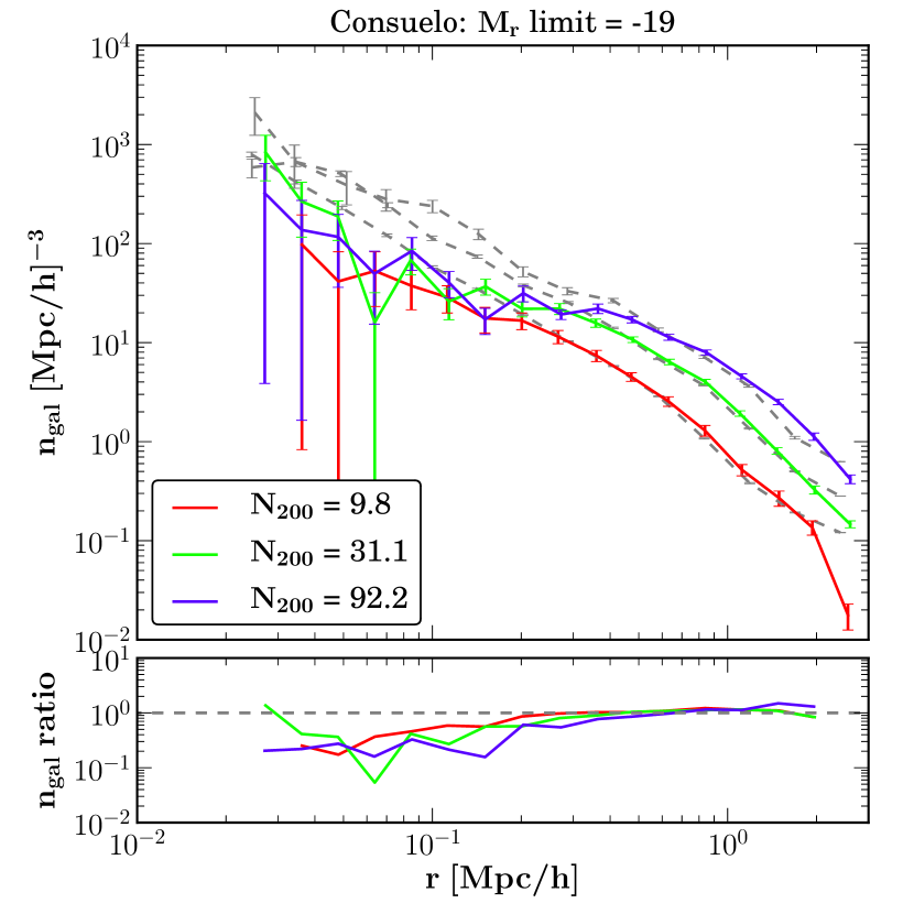
Figure 8: Galaxy number density profile from the Consuelo simulation. The colored curves show galaxies in the simulation, while the grey dashed curves correspond to the observations of SDSS from Tinker et al. (2012). As can be seen, the simulated galaxy population near the centre of clusters tend to have a shallower distribution than the real galaxy population. The difference is larger for more massive clusters. This figure is adapted from Wu et al. (in preparation).

Fig. 8 presents the galaxy number density profile based on which we model its theoretical uncertainties. The colored curves are based on the Consuelo simulation – an $\displaystyle N$-body simulation with $\displaystyle 1400^{3}$ particles in a volume of side length $\displaystyle 420\,h^{-1}\rm M_{\odot}$. The mass resolution is $\displaystyle 1.9\times 10^{9}\,h^{-1}\rm M_{\odot}$, and the force resolution is $\displaystyle 8\,h^{-1}\rm kpc$. We assign each subhalo a luminosity value using the $\displaystyle v_{\rm max}^{\rm pk}$–luminosity relation based on a subhalo abundance matching model (Behroozi, private communication), where $\displaystyle v_{\rm max}^{\rm pk}$ is the subhalo’s peak maximum circular velocity in its history.

We compare the simulated galaxy density profiles with the results from the SDSS maxBCG cluster catalogue as presented in Tinker et al. (2012). The grey dashed curves correspond to three of the richness bins of maxBCG. From the Consuelo simulation, we select clusters in a way that they have approximately the same mass distribution as the maxBCG cluster sample (Johnston et al., 2007). Each maxBCG cluster is assigned a richness value $\displaystyle N_{200}$, which is the number of red-sequence galaxies brighter than ${}^{0.25}M_{i}=-19.2$ within $\displaystyle r_{200}$. Here $\displaystyle r_{200}$ is defined as the radius within which the density of galaxies is 200 times the mean density of galaxies. At large radii ($\displaystyle>0.5\,h^{-1}\rm Mpc$), the simulation and observation agree well. This agreement naturally comes from our mass selection and abundance matching without tuning the normalization.

However, discrepancy between simulation and observation occurs at small radius. As can be seen, the subhalo number density profile measured from the simulation is shallower than the galaxy density profile measured from SDSS and is also shallower than the NFW profile. This discrepancy is stronger for more massive host haloes. Wu et al. (in preparation) further demonstrate that (1) the discrepancy is also stronger for dimmer galaxies, (2) the trend exists in several state-of-the-art $\displaystyle N$-body simulations using different algorithms and resolutions, and (3) the incompleteness of subhaloes depends on the radius, the mass of the host halo and the mass of the subhalo. It has been shown that the deficit of simulated galaxies near the centre of massive haloes can be alleviated in hydrodynamical simulations that include cooling and star formation (e.g., Weinberg et al., 2008; Dolag et al., 2009). Therefore, it is highly likely that this deficit presents a fundamental limitation of $\displaystyle N$-body simulations and needs to be taken into account when we use $\displaystyle N$-body simulations to model the galaxy population in massive clusters.

Appendix B Derivation of the galaxy power spectrum

In this appendix, we provide the detailed derivation of the galaxy power spectrum, mainly following the derivations in Scherrer & Bertschinger (1991), Seljak (2000) and Cooray & Sheth (2002), in order to clarify possible confusions originated from different conventions. Let us assume that dark matter halo $\displaystyle i$ with mass $\displaystyle M_{i}$ is located at $\displaystyle{\bm{x}}_{i}$. It has $\displaystyle N_{i}$ galaxies, whose spatial distribution is described by $\displaystyle u({\bm{x}}-{\bm{x}}_{i}|M_{i})$ [normalized so that $\displaystyle\int{\rm d}^{3}{\bm{x}}\ u({\bm{x}}|M)=1$]. The galaxy number density field can be described by summing over all haloes in the universe:

$${n_{\rm gal}}({\bm{x}})=\sum_{i}N_{i}\ u({\bm{x}}-{\bm{x}}_{i}|M_{i})$$ (44)

$$=\sum_{i}\int dM\delta_{D}(M-M_{i})\int{\rm d}^{3}{\bm{x}}^{\prime}\delta_{D}({\bm{x}}^{\prime}-{\bm{x}}_{i})N_{i}u\left({\bm{x}}-{\bm{x}}^{\prime}|M\right),$$

where we insert Dirac delta functions for $\displaystyle M$ and $\displaystyle{\bm{x}}^{\prime}$. If we define

$$\left\langle\sum_{i}\delta_{D}(M-M_{i})\delta_{D}({\bm{x}}^{\prime}-{\bm{x}}_{i})\ N_{i}\right\rangle\equiv n(M)\left\langle{N|M}\right\rangle\ ,$$ (45)

then the mean galaxy number density is given by

$${{{\bar{n}}_{\rm gal}}}=\left\langle{{n_{\rm gal}}}\right\rangle=\int dMn(M)\left\langle{N|M}\right\rangle\ ,$$ (46)

where we write $\displaystyle n(M)$ = $\displaystyle{dn}/{dM}$ for the halo mass function.

The number density fluctuation of galaxies is defined as

$${\delta_{\rm gal}}({\bm{x}})=\frac{{n_{\rm gal}}({\bm{x}})}{{{\bar{n}}_{\rm gal}}}-1\ .$$ (47)

The two-point statistics follows the definition:

$$\left\langle\sum_{i}\delta_{D}(M_{1}-M_{i})\delta_{D}({\bm{x}}_{1}-{\bm{x}}_{i})N_{i}\sum_{j}\delta_{D}(M_{2}-M_{j})\delta_{D}({\bm{x}}_{2}-{\bm{x}}_{j})N_{j}\right\rangle$$ (48)

$$\equiv n(M_{1})\left\langle{N|M_{1}}\right\rangle n(M_{2})\left\langle{N|M_{2}}\right\rangle\left[1+\xi_{\rm hh}(M_{1},M_{2},|{\bm{x}}_{2}-{\bm{x}}_{1}|)\right]\quad(i\neq j)$$

$$+n(M_{1})\left\langle{{N\choose 2}|M_{1}}\right\rangle\delta_{D}(M_{1}-M_{2})\delta_{D}({\bm{x}}_{1}-{\bm{x}}_{2})\quad(i=j)\ ,$$

where $\displaystyle\xi_{\rm hh}$ is the two-point correlation function of dark matter contributed by two different haloes. The two-point correlation function for galaxies reads

$$\xi_{\rm gg}(r)=\left\langle{{\delta_{\rm gal}}({\bm{x}}){\delta_{\rm gal}}({\bm{x}}+{\bm{r}})}\right\rangle$$ (49)

$$=\frac{1}{{{\bar{n}}_{\rm gal}}^{2}}\int dM_{1}\int dM_{2}\int{\rm d}^{3}{\bm{x}}_{1}\int{\rm d}^{3}{\bm{x}}_{2}\ u({\bm{x}}-{\bm{x}}_{1}|M_{1})u({\bm{x}}+{\bm{r}}-{\bm{x}}_{2}|M_{2})$$

$$\left\langle\sum_{i}\delta_{D}(M_{1}-M_{i})\delta_{D}({\bm{x}}_{1}-{\bm{x}}_{i})N_{i}\sum_{j}\delta_{D}(M_{2}-M_{j})\delta_{D}({\bm{x}}_{2}-{\bm{x}}_{j})N_{j}\right\rangle$$

$$=\xi_{\rm gg}^{\rm 1h}(r)+\xi_{\rm gg}^{\rm 2h}(r)\ ,$$

where

$$\xi_{\rm gg}^{\rm 1h}(r)=\frac{1}{{{\bar{n}}_{\rm gal}}^{2}}\int dMn(M)\left\langle{\textstyle{N\choose 2}|M}\right\rangle\int{\rm d}^{3}{\bm{x}}\ u({\bm{x}}|M)u({\bm{x}}+{\bm{r}}|M)\ ,$$ (50)

$$\xi_{\rm gg}^{\rm 2h}(r)=\frac{1}{{{\bar{n}}_{\rm gal}}^{2}}\int dM_{1}n(M_{1})\left\langle{N|M_{1}}\right\rangle\int dM_{2}n(M_{2})\left\langle{N|M_{2}}\right\rangle$$

$$\int{\rm d}^{3}{\bm{x}}_{1}\int{\rm d}^{3}{\bm{x}}_{2}u({\bm{x}}_{1}|M_{1})u({\bm{x}}_{2}-{\bm{r}}|M_{2})(1+\xi_{\rm hh}(M_{1},M_{2};|{\bm{x}}_{2}-{\bm{x}}_{1}-{\bm{r}}|))\ .$$

We now turn to the Fourier space. We follow this convention of the Fourier transform

$$\tilde{\delta}({\bm{k}})=\frac{1}{\sqrt{V}}\int{\rm d}^{3}{\bm{x}}\ \delta({\bm{x}})\ {\rm e}^{-i{\bm{k}}\cdot{\bm{x}}}\ .$$ (51)

The Dirac delta function in k-space is defined as

$$\delta_{D}({\bm{k}})=\frac{1}{V}\int\frac{{\rm d}^{3}{\bm{x}}}{(2{\rm\pi})^{3}}\ {\rm e}^{-i{\bm{k}}\cdot{\bm{x}}}\quad\mbox{(dimensionless)}\ .$$ (52)

From this convention, the relation between the correlation function and the power spectrum follows:

$$\xi(r)=\frac{1}{(2{\rm\pi})^{3}}\int{\rm d}^{3}{\bm{k}}P({\bm{k}}){\rm e}^{-i{\bm{k}}\cdot{\bm{r}}}\ .$$ (53)

The Fourier transform of the density perturbation reads

$${\tilde{\delta}_{\rm gal}}({\bm{k}}) =\frac{1}{\sqrt{V}}\int{\rm d}^{3}{\bm{x}}\ {\delta_{\rm gal}}({\bm{x}})\ {\rm e}^{-i{\bm{k}}\cdot{\bm{x}}}$$ (54)

$$=\frac{1}{{{\bar{n}}_{\rm gal}}\sqrt{V}}\sum_{i}N_{i}{\tilde{u}}({\bm{k}}|M_{i}){\rm e}^{-i{\bm{k}}\cdot{\bm{x}}_{i}}-{(2{\rm\pi})^{3}}{\sqrt{V}}\delta_{D}({\bm{k}})\ ,$$

where

$${\tilde{u}}({\bm{k}}|M)=\int{\rm d}^{3}{\bm{x}}u({\bm{x}}|M){\rm e}^{-i{\bm{k}}\cdot{\bm{x}}}\ .$$ (55)

Based on this definition, $\displaystyle{\tilde{u}}\rightarrow 1$ when $\displaystyle k\rightarrow 0$ and is dimensionless. Applying the Fourier transform to equation (48), we obtain

$$\left\langle\sum_{i}\delta_{D}(M_{1}-M_{i}){\rm e}^{-i{\bm{k}}_{1}\cdot{\bm{x}}_{i}}N_{i}\sum_{j}\delta_{D}(M_{2}-M_{j}){\rm e}^{+i{\bm{k}}_{2}\cdot{\bm{x}}_{j}}N_{j}\right\rangle$$ (56)

$$\equiv n(M_{1})\left\langle{N|M_{1}}\right\rangle n(M_{2})\left\langle{N|M_{2}}\right\rangle(2{\rm\pi})^{6}V^{2}\delta_{D}({\bm{k}}_{1})\delta_{D}({\bm{k}}_{2})$$

$$+(2{\rm\pi})^{3}Vn(M_{1})\left\langle{N|M_{1}}\right\rangle n(M_{2})\left\langle{N|M_{2}}\right\rangle P_{\rm hh}(M_{1},M_{2};k)\delta_{D}({\bm{k}}_{1}-{\bm{k}}_{2})$$

$$+(2{\rm\pi})^{3}Vn(M_{1})\left\langle{\textstyle{N\choose 2}|M_{1}}\right\rangle\delta_{D}(M_{1}-M_{2})\delta_{D}({\bm{k}}_{1}-{\bm{k}}_{2})$$

We note that under our convention of the Fourier transform, $\displaystyle\int{\rm d}^{3}{\bm{k}}\delta_{D}({\bm{k}})=1/V$ and $\displaystyle\delta_{D}({\bm{k}})\delta_{D}({\bm{k}})=\delta_{D}({\bm{k}})/(2{\rm\pi})^{3}$.

We are now ready to compute the galaxy power spectrum. Applying the trick of inserting Dirac delta functions and then using equation (LABEL:eq:2pt_k), we obtain

$$P_{\rm gg}(k)=\frac{1}{(2{\rm\pi})^{3}}\left\langle{{\tilde{\delta}_{\rm gal}}({\bm{k}}){\tilde{\delta}_{\rm gal}}^{*}({\bm{k}})}\right\rangle$$ (57)

$$=\frac{1}{(2{\rm\pi})^{3}V{{{\bar{n}}_{\rm gal}}}^{2}}\left\langle\sum_{i}{\tilde{u}}({\bm{k}}|M_{i}){\rm e}^{-i{\bm{k}}\cdot{\bm{x}}_{i}}N_{i}\sum_{j}{\tilde{u}}^{*}({\bm{k}}|M_{j}){\rm e}^{i{\bm{k}}\cdot{\bm{x}}_{j}}N_{j}\right\rangle$$

$$=P_{\rm gg}^{\rm 1h}(k)+P_{\rm gg}^{\rm 2h}(k)\ ,$$

where the two-halo term reads

$$P_{\rm gg}^{\rm 2h}(k)=\left[\frac{1}{{{{\bar{n}}_{\rm gal}}}}\int dM\frac{dn}{dM}\left\langle{N|M}\right\rangle b(M)\right]^{2}P_{\rm lin}(k)\ ,$$ (58)

and the one-halo term reads

$$P_{\rm gg}^{\rm 1h}(k)=\frac{1}{{{{\bar{n}}_{\rm gal}}}^{2}}\int dM\frac{dn}{dM}\left\langle{\displaystyle{\left.N\choose 2\right|}M}\right\rangle f(k|M)\ .$$ (59)

Here $\displaystyle\left\langle{\textstyle{\left.N\choose 2\right|}M}\right\rangle f(k|M)$ is the galaxy pair-weighted profile, including the contribution from central and satellite galaxies (Berlind & Weinberg, 2002)

$$\left\langle{{\left.N\choose 2\right|}M}\right\rangle f(k|M)$$ (60)

$$=\left[\left\langle{N_{\rm sat}|M}\right\rangle{\tilde{u}}(k|M)+\frac{1}{2}\left\langle{N_{\rm sat}(N_{\rm sat}-1)|M}\right\rangle|{\tilde{u}}(k|M)|^{2}\right]\ .$$

Appendix C Derivation of the covariance matrix

We now derive the covariance of power spectra at different wave numbers in equation (17). First, recall the definitions for power spectrum and trispectrum:

$$\left\langle{\delta({\bm{k}}_{1})\delta({\bm{k}}_{2})}\right\rangle =(2{\rm\pi})^{3}\delta_{D}({\bm{k}}_{12})P(k_{1})$$ (61)

$$\left\langle{\delta({\bm{k}}_{1})\delta({\bm{k}}_{2})\delta({\bm{k}}_{3})\delta({\bm{k}}_{4})}\right\rangle_{c} =(2{\rm\pi})^{3}\delta_{D}({\bm{k}}_{1234})T(k_{1},k_{2},k_{3},k_{4})\ ,$$

where the subscript $\displaystyle c$ indicates the “connected” term. Under our convention, $\displaystyle[P]=L^{3}$ and $\displaystyle[T]=L^{6}$. For a given realization of the density field $\displaystyle\delta({\bm{k}})$, the estimator of the binned power spectrum is

$$\hat{P}(k_{i})=\int_{k_{i}}\frac{{\rm d}^{3}{\bm{k}}}{V_{s}(k_{i})}\delta({\bm{k}})\delta(-{\bm{k}})\ ,$$ (62)

where $\displaystyle V_{s}(k_{i})=4{\rm\pi}k_{i}^{3}\delta\ln k$. Its covariance is

$$C_{ij} =\left\langle{\hat{P}(k_{i})\hat{P}(k_{j})}\right\rangle-\left\langle{\hat{P}(k_{i})}\right\rangle\left\langle{\hat{P}(k_{j})}\right\rangle$$ (63)

$$=\frac{(2{\rm\pi})^{3}}{V}\frac{2P(k_{i})^{2}}{V_{s}(k_{i})}\delta_{ij}+\bar{T}(k_{i},k_{j})\ ,$$

where

$$\bar{T}(k_{i},k_{j})\equiv\int_{k_{i}}\frac{{\rm d}^{3}{\bm{k}}_{1}}{V_{s}(k_{i})}\int_{k_{j}}\frac{{\rm d}^{3}{\bm{k}}_{2}}{V_{s}(k_{j})}T({\bm{k}}_{1},-{\bm{k}}_{1},{\bm{k}}_{2},-{\bm{k}}_{2})\ .$$ (64)

Below we provide the derivation. The first term in equation (63) can be calculated as

$$\left\langle{\hat{P}(k_{i})\hat{P}(k_{j})}\right\rangle=\int_{k_{i}}\frac{{\rm d}^{3}{\bm{k}}_{1}}{V_{s}(k_{i})}\int_{k_{j}}\frac{{\rm d}^{3}{\bm{k}}_{2}}{V_{s}(k_{j})}\left\langle{\delta({\bm{k}}_{1})\delta(-{\bm{k}}_{1})\delta({\bm{k}}_{2})\delta(-{\bm{k}}_{2})}\right\rangle\ ,$$ (65)

where the integrand reads:

$$\displaystyle\left\langle{\delta({\bm{k}}_{1})\delta(-{\bm{k}}_{1})\delta({\bm{k}}_{2})\delta(-{\bm{k}}_{2})}\right\rangle$$

$$\displaystyle=\left\langle{\delta_{1}\delta_{1}^{*}\delta_{2}\delta_{2}^{*}}\right\rangle_{c}+\left\langle{\delta_{1}\delta_{1}^{*}}\right\rangle\left\langle{\delta_{2}\delta_{2}^{*}}\right\rangle+\left\langle{\delta_{1}\delta_{2}}\right\rangle\left\langle{\delta_{1}^{*}\delta_{2}^{*}}\right\rangle+\left\langle{\delta_{1}\delta_{2}^{*}}\right\rangle\left\langle{\delta_{2}\delta_{1}^{*}}\right\rangle$$

$$\displaystyle=(2{\rm\pi})^{3}\delta_{D}(0)T({\bm{k}}_{1},-{\bm{k}}_{1},{\bm{k}}_{2},-{\bm{k}}_{2})$$ (66)

$$\displaystyle+(2{\rm\pi})^{6}\delta_{D}(0)P({\bm{k}}_{1})\delta(0)P({\bm{k}}_{2})$$ (67)

$$\displaystyle+(2{\rm\pi})^{6}\delta_{D}({\bm{k}}_{1}+{\bm{k}}_{2})P({\bm{k}}_{1})\delta({\bm{k}}_{1}+{\bm{k}}_{2})P({\bm{k}}_{1})$$ (68)

$$\displaystyle+(2{\rm\pi})^{6}\delta_{D}({\bm{k}}_{1}-{\bm{k}}_{2})P({\bm{k}}_{1})\delta({\bm{k}}_{1}-{\bm{k}}_{2})P({\bm{k}}_{1})\ .$$ (69)

We note that $\displaystyle\delta_{D}(0)=\frac{1}{(2{\rm\pi})^{3}}$ . Then the contribution from each term reads

(66) $$\Rightarrow\int_{k_{i}}\frac{{\rm d}^{3}{\bm{k}}_{1}}{V_{s}(k_{i})}\int_{k_{j}}\frac{{\rm d}^{3}{\bm{k}}_{2}}{V_{s}(k_{j})}T({\bm{k}}_{1},-{\bm{k}}_{1},{\bm{k}}_{2},-{\bm{k}}_{2})\equiv\bar{T}(k_{i},k_{j})$$ (70)

(67) $$\Rightarrow\left\langle{\hat{P}(k_{i})}\right\rangle\left\langle{\hat{P}(k_{j})}\right\rangle$$

   (cancels the second term of equation (63))

$$\mbox{(\ref{eq:iii})}=\mbox{(\ref{eq:iv})} \Rightarrow\int_{k_{i}}\frac{{\rm d}^{3}{\bm{k}}_{1}}{V_{s}(k_{i})}\int_{k_{j}}\frac{{\rm d}^{3}{\bm{k}}_{2}}{V_{s}(k_{j})}(2{\rm\pi})^{3}\delta_{D}({\bm{k}}_{1}-{\bm{k}}_{2})P({\bm{k}}_{1})P({\bm{k}}_{1})$$

$$=\int_{k_{i}}\frac{{\rm d}^{3}{\bm{k}}_{1}}{V_{s}(k_{i})}P(k_{1})^{2}(2{\rm\pi})^{3}\int_{k_{j}}\frac{{\rm d}^{3}{\bm{k}}_{2}}{V_{s}(k_{j})}\delta_{D}({\bm{k}}_{1}-{\bm{k}}_{2})$$

   (only non-zero if $$k_{i}=k_{j}$$)

$$={\frac{(2{\rm\pi})^{3}}{V_{z}}\frac{\left\langle{\hat{P}(k_{i})^{2}}\right\rangle}{V_{s}(k_{i})}\delta_{ij}}\approx\frac{(2{\rm\pi})^{3}}{V_{z}}\frac{P(k_{i})^{2}}{V_{s}(k_{i})}\delta_{ij}$$

The expression of $\displaystyle\bar{T}(k_{i},k_{j})$ (equation 19) can be obtained using equation (54) and is similar to the derivation of $\displaystyle P(k)$.

References

- Abazajian et al. (2005) Abazajian K., et al., 2005, ApJ, 625, 613
- Albrecht et al. (2006) Albrecht A., et al., 2006, arXiv:astro-ph/0609591
- Anderson et al. (2012) Anderson L., et al., 2012, MNRAS, 427, 3435
- Berlind & Weinberg (2002) Berlind A. A., Weinberg D. H., 2002, ApJ, 575, 587
- Bernstein & Huterer (2010) Bernstein G., Huterer D., 2010, MNRAS, 401, 1399
- Bhattacharya et al. (2013) Bhattacharya S., Habib S., Heitmann K., Vikhlinin A., 2013, ApJ, 766, 32
- Blake et al. (2011) Blake C., et al., 2011, MNRAS, 418, 1707
- Blake & Glazebrook (2003) Blake C., Glazebrook K., 2003, ApJ, 594, 665
- Boylan-Kolchin et al. (2010) Boylan-Kolchin M., Springel V., White S. D. M., Jenkins A., 2010, MNRAS, 406, 896
- Bullock et al. (2001) Bullock J. S., Kolatt T. S., Sigad Y., Somerville R. S., Kravtsov A. V., Klypin A. A., Primack J. R., Dekel A., 2001, MNRAS, 321, 559
- Cacciato et al. (2013) Cacciato M., van den Bosch F. C., More S., Mo H., Yang X., 2013, MNRAS, 430, 767
- Chuang & Wang (2012) Chuang C.-H., Wang Y., 2012, MNRAS, 426, 226
- Coe et al. (2012) Coe D., et al., 2012, ApJ, 757, 22
- Cohn & White (2008) Cohn J. D., White M., 2008, MNRAS, 385, 2025
- Cole et al. (2005) Cole S., et al., 2005, MNRAS, 362, 505
- Cole et al. (2000) Cole S., Lacey C. G., Baugh C. M., Frenk C. S., 2000, MNRAS, 319, 168
- Colín et al. (2000) Colín P., Klypin A. A., Kravtsov A. V., 2000, ApJ, 539, 561
- Colless et al. (2001) Colless M., et al., 2001, MNRAS, 328, 1039
- Contreras et al. (2013) Contreras S., Baugh C. M., Norberg P., Padilla N., 2013, MNRAS, 432, 2717
- Cooray & Hu (2001) Cooray A., Hu W., 2001, ApJ, 554, 56
- Cooray & Sheth (2002) Cooray A., Sheth R., 2002, Phys. Rep., 372, 1
- Coupon et al. (2012) Coupon J., et al., 2012, A&A, 542, A5
- Crocce et al. (2010) Crocce M., Fosalba P., Castander F. J., Gaztañaga E., 2010, MNRAS, 403, 1353
- Cui et al. (2012) Cui W., Borgani S., Dolag K., Murante G., Tornatore L., 2012, MNRAS, 423, 2279
- Cunha & Evrard (2010) Cunha C. E., Evrard A. E., 2010, Phys. Rev. D, 81, 083509
- Dalal et al. (2008) Dalal N., Doré O., Huterer D., Shirokov A., 2008, Phys. Rev. D, 77, 123514
- de la Torre & Guzzo (2012) de la Torre S., Guzzo L., 2012, MNRAS, 427, 327
- Diemand et al. (2004) Diemand J., Moore B., Stadel J., 2004, MNRAS, 352, 535
- Dolag et al. (2009) Dolag K., Borgani S., Murante G., Springel V., 2009, MNRAS, 399, 497
- Drinkwater et al. (2010) Drinkwater M. J., et al., 2010, MNRAS, 401, 1429
- Duffy et al. (2008) Duffy A. R., Schaye J., Kay S. T., Dalla Vecchia C., 2008, MNRAS, 390, L64
- Duffy et al. (2010) Duffy A. R., Schaye J., Kay S. T., Dalla Vecchia C., Battye R. A., Booth C. M., 2010, MNRAS, 405, 2161
- Eisenstein et al. (2005) Eisenstein D. J., et al., 2005, ApJ, 633, 560
- Evrard et al. (2002) Evrard A. E., et al., 2002, ApJ, 573, 7
- Evrard et al. (2008) Evrard A. E., et al., 2008, ApJ, 672, 122
- Faltenbacher & Diemand (2006) Faltenbacher A., Diemand J., 2006, MNRAS, 369, 1698
- Gao et al. (2004) Gao L., De Lucia G., White S. D. M., Jenkins A., 2004, MNRAS, 352, L1
- Geller & Huchra (1989) Geller M. J., Huchra J. P., 1989, Sci, 246, 897
- Groth & Peebles (1977) Groth E. J., Peebles P. J. E., 1977, ApJ, 217, 385
- Guo et al. (2011) Guo Q., et al., 2011, MNRAS, 413, 101
- Heitmann et al. (2010) Heitmann K., White M., Wagner C., Habib S., Higdon D., 2010, ApJ, 715, 104
- Hu & Kravtsov (2003) Hu W., Kravtsov A. V., 2003, ApJ, 584, 702
- Huchra et al. (1983) Huchra J., Davis M., Latham D., Tonry J., 1983, ApJS, 52, 89
- Huterer & Turner (2001) Huterer D., Turner M. S., 2001, Phys. Rev. D, 64, 123527
- Jenkins et al. (2001) Jenkins A., Frenk C. S., White S. D. M., Colberg J. M., Cole S., Evrard A. E., Couchman H. M. P., Yoshida N., 2001, MNRAS, 321, 372
- Jennings et al. (2011) Jennings E., Baugh C. M., Pascoli S., 2011, MNRAS, 410, 2081
- Johnston et al. (2007) Johnston D. E., et al., 2007, arXiv:0709.1159
- Kaiser (1987) Kaiser N., 1987, MNRAS, 227, 1
- Kauffmann et al. (1993) Kauffmann G., White S. D. M., Guiderdoni B., 1993, MNRAS, 264, 201
- Knox et al. (1998) Knox L., Scoccimarro R., Dodelson S., 1998, Physical Review Letters, 81, 2004
- Komatsu et al. (2011) Komatsu E., et al., 2011, ApJS, 192, 18
- Kravtsov et al. (2004) Kravtsov A. V., Berlind A. A., Wechsler R. H., Klypin A. A., Gottlöber S., Allgood B., Primack J. R., 2004, ApJ, 609, 35
- Kwan et al. (2013) Kwan J., Bhattacharya S., Heitmann K., Habib S., 2013, ApJ, 768, 123
- Kwan et al. (2012) Kwan J., Lewis G. F., Linder E. V., 2012, ApJ, 748, 78
- Lau et al. (2009) Lau E. T., Kravtsov A. V., Nagai D., 2009, ApJ, 705, 1129
- Lau et al. (2010) Lau E. T., Nagai D., Kravtsov A. V., 2010, ApJ, 708, 1419
- Le Fèvre et al. (2005) Le Fèvre O., et al., 2005, A&A, 439, 845
- Linder & Samsing (2013) Linder E. V., Samsing J., 2013, J. Cosmol. Astropart. Phys., 2, 25
- Lukić et al. (2007) Lukić Z., Heitmann K., Habib S., Bashinsky S., Ricker P. M., 2007, ApJ, 671, 1160
- Lukić et al. (2009) Lukić Z., Reed D., Habib S., Heitmann K., 2009, ApJ, 692, 217
- Ma et al. (2011) Ma C.-P., Maggiore M., Riotto A., Zhang J., 2011, MNRAS, 411, 2644
- Macciò et al. (2008) Macciò A. V., Dutton A. A., van den Bosch F. C., 2008, MNRAS, 391, 1940
- Macciò et al. (2006) Macciò A. V., Moore B., Stadel J., Diemand J., 2006, MNRAS, 366, 1529
- Maddox et al. (1990) Maddox S. J., Efstathiou G., Sutherland W. J., Loveday J., 1990, MNRAS, 242, 43P
- Manera & Gaztañaga (2011) Manera M., Gaztañaga E., 2011, MNRAS, 415, 383
- Marín et al. (2013) Marín F. A., et al., 2013, MNRAS, 432, 2654
- Miller et al. (2001) Miller C. J., Nichol R. C., Batuski D. J., 2001, ApJ, 555, 68
- Munari et al. (2013) Munari E., Biviano A., Borgani S., Murante G., Fabjan D., 2013, MNRAS, 430, 2638
- Nagai & Kravtsov (2005) Nagai D., Kravtsov A. V., 2005, ApJ, 618, 557
- Navarro et al. (1997) Navarro J. F., Frenk C. S., White S. D. M., 1997, ApJ, 490, 493
- Neto et al. (2007) Neto A. F., et al., 2007, MNRAS, 381, 1450
- Oguri et al. (2012) Oguri M., Bayliss M. B., Dahle H., Sharon K., Gladders M. D., Natarajan P., Hennawi J. F., Koester B. P., 2012, MNRAS, 420, 3213
- Paranjape et al. (2013) Paranjape A., Sheth R. K., Desjacques V., 2013, MNRAS, 431, 1503
- Parkinson et al. (2012) Parkinson D., et al., 2012, Phys. Rev. D, 86, 103518
- Peacock (1999) Peacock J. A., 1999, Cosmological Physics. Cambridge University Press, Cambridge, UK
- Peacock & Dodds (1994) Peacock J. A., Dodds S. J., 1994, MNRAS, 267, 1020
- Peacock & Smith (2000) Peacock J. A., Smith R. E., 2000, MNRAS, 318, 1144
- Percival et al. (2010) Percival W. J., et al., 2010, MNRAS, 401, 2148
- Planck Collaboration (2013) Planck Collaboration 2013, arXiv:1303.5084
- Prada et al. (2012) Prada F., Klypin A. A., Cuesta A. J., Betancort-Rijo J. E., Primack J., 2012, MNRAS, 423, 3018
- Press & Schechter (1974) Press W. H., Schechter P., 1974, ApJ, 187, 425
- Rasia et al. (2013) Rasia E., Borgani S., Ettori S., Mazzotta P., Meneghetti M., 2013, arXiv:1301.7476
- Reed et al. (2003) Reed D., Gardner J., Quinn T., Stadel J., Fardal M., Lake G., Governato F., 2003, MNRAS, 346, 565
- Reed et al. (2013) Reed D. S., Smith R. E., Potter D., Schneider A., Stadel J., Moore B., 2013, MNRAS, 431, 1866
- Reid et al. (2010) Reid B. A., et al., 2010, MNRAS, 404, 60
- Rozo et al. (2010) Rozo E., et al., 2010, ApJ, 708, 645
- Rudd et al. (2008) Rudd D. H., Zentner A. R., Kravtsov A. V., 2008, ApJ, 672, 19
- Scherrer & Bertschinger (1991) Scherrer R. J., Bertschinger E., 1991, ApJ, 381, 349
- Schlegel et al. (2009) Schlegel D., White M., Eisenstein D., 2009, arXiv:0902.4680
- Scoccimarro et al. (2001) Scoccimarro R., Sheth R. K., Hui L., Jain B., 2001, ApJ, 546, 20
- Scoccimarro et al. (1999) Scoccimarro R., Zaldarriaga M., Hui L., 1999, ApJ, 527, 1
- Seljak (2000) Seljak U., 2000, MNRAS, 318, 203
- Seljak (2001) Seljak U., 2001, MNRAS, 325, 1359
- Seljak (2009) Seljak U., 2009, Phys. Rev. Lett., 102, 021302
- Seo & Eisenstein (2003) Seo H.-J., Eisenstein D. J., 2003, ApJ, 598, 720
- Sheth et al. (2001) Sheth R. K., Mo H. J., Tormen G., 2001, MNRAS, 323, 1
- Sheth & Tormen (1999) Sheth R. K., Tormen G., 1999, MNRAS, 308, 119
- Simha et al. (2012) Simha V., Weinberg D. H., Davé R., Fardal M., Katz N., Oppenheimer B. D., 2012, MNRAS, 423, 3458
- Smith et al. (2003) Smith R. E., et al., 2003, MNRAS, 341, 1311
- Smith et al. (2012) Smith R. E., Reed D. S., Potter D., Marian L., Crocce M., Moore B., 2012, arXiv:1211.6434
- Smith et al. (2007) Smith R. E., Scoccimarro R., Sheth R. K., 2007, Phys. Rev. D, 75, 063512
- Somerville & Primack (1999) Somerville R. S., Primack J. R., 1999, MNRAS, 310, 1087
- Stanek et al. (2010) Stanek R., Rasia E., Evrard A. E., Pearce F., Gazzola L., 2010, ApJ, 715, 1508
- Tegmark et al. (2006) Tegmark M., et al., 2006, Phys. Rev. D, 74, 123507
- Tinker et al. (2012) Tinker J. L., et al., 2012, ApJ, 745, 16
- Tinker et al. (2008) Tinker J. L., Kravtsov A. V., Klypin A., Abazajian K., Warren M., Yepes G., Gottlöber S., Holz D. E., 2008, ApJ, 688, 709
- Tinker et al. (2010) Tinker J. L., Robertson B. E., Kravtsov A. V., Klypin A., Warren M. S., Yepes G., Gottlöber S., 2010, ApJ, 724, 878
- Tinker et al. (2005) Tinker J. L., Weinberg D. H., Zheng Z., Zehavi I., 2005, ApJ, 631, 41
- Vale & Ostriker (2004) Vale A., Ostriker J. P., 2004, MNRAS, 353, 189
- van den Bosch et al. (2007) van den Bosch F. C., et al., 2007, MNRAS, 376, 841
- Wang et al. (2006) Wang L., Li C., Kauffmann G., De Lucia G., 2006, MNRAS, 371, 537
- Warren et al. (2006) Warren M. S., Abazajian K., Holz D. E., Teodoro L., 2006, ApJ, 646, 881
- Watson et al. (2013) Watson W. A., Iliev I. T., D’Aloisio A., Knebe A., Shapiro P. R., Yepes G., 2013, MNRAS, 433, 1230
- Weinberg et al. (2008) Weinberg D. H., Colombi S., Davé R., Katz N., 2008, ApJ, 678, 6
- Wetzel & White (2010) Wetzel A. R., White M., 2010, MNRAS, 403, 1072
- White (2001) White M., 2001, MNRAS, 321, 1
- White & Frenk (1991) White S. D. M., Frenk C. S., 1991, ApJ, 379, 52
- Wu et al. (2013) Wu H.-Y., Hahn O., Evrard A. E., Wechsler R. H., Dolag K., 2013b, arXiv:1307.0011
- Wu et al. (2013) Wu H.-Y., Hahn O., Wechsler R. H., Behroozi P. S., Mao Y.-Y., 2013a, ApJ, 767, 23
- Wu et al. (2010) Wu H.-Y., Zentner A. R., Wechsler R. H., 2010, ApJ, 713, 856
- Xu et al. (2013) Xu X., Cuesta A. J., Padmanabhan N., Eisenstein D. J., McBride C. K., 2013, MNRAS, 431, 2834
- York et al. (2000) York D. G., et al., 2000, AJ, 120, 1579
- Zehavi et al. (2011) Zehavi I., et al., 2011, ApJ, 736, 59
- Zheng et al. (2005) Zheng Z., et al., 2005, ApJ, 633, 791
- Zheng & Weinberg (2007) Zheng Z., Weinberg D. H., 2007, ApJ, 659, 1