Multi-Pair Amplify-and-Forward Relaying with Very Large Antenna Arrays

Abstract

We consider a multi-pair relay channel where multiple sources simultaneously communicate with destinations using a relay. Each source or destination has only a single antenna, while the relay is equipped with a very large antenna array. We investigate the power efficiency of this system when maximum ratio combining/maximal ratio transmission (MRC/MRT) or zero-forcing (ZF) processing is used at the relay. Using a very large array, the transmit power of each source or relay (or both) can be made inversely proportional to the number of relay antennas while maintaining a given quality-of-service. At the same time, the achievable sum rate can be increased by a factor of the number of source-destination pairs. We show that when the number of antennas grows to infinity, the asymptotic achievable rates of MRC/MRT and ZF are the same if we scale the power at the sources. Depending on the large scale fading effect, MRC/MRT can outperform ZF or vice versa if we scale the power at the relay.

I Introduction

Multiple-input multiple-output (MIMO) technology has now become an integral feature of many advanced communication systems. A cellular architecture with MIMO that has gained significant research interest is multi-user MIMO (MU-MIMO) in which an antenna array simultaneously serves a multiplicity of autonomous co-channel users/nodes [1]. While the current systems have limited number of antennas (e.g. the LTE standard allows for up to $8$ antenna ports), MU systems having a large number of antennas at the base station (very large MIMO) have been advocated recently in [2, 3, 4]. Very large MU-MIMO systems can substantially reduce the interference with simple signal processing techniques and achieve increased reliability and throughput, and significant reduction in total transmitted power [5].

On the other hand, relaying has been extensively explored to provide expanded coverage and high throughput, especially at the cell edge [6]. However, inter-user interference can cause major performance degradation in MU relay systems [7]. As a result, a large body of performance analysis work on MU relay systems, e.g., [8, 9, 10] has mainly avoided interference slots by adopting spectrally inefficient policies such as orthogonalization of time/frequency. Another line of work on MU relay systems has considered deploying complicated precoder/decoder designs; e.g., in [11] and advanced joint network coding and signal alignment techniques for the multi-pair two-way relay channel [12].

In this paper, we analyze the performance of a multi-pair relaying scenario where a group of $K$ sources and $K$ destinations communicate using a single relay equipped with $N$ antennas, where $N\gg K$. To the best of our knowledge, there is no prior work that analyzes the effects of large antenna arrays on the performance of the considered relay system. In the first time slot, all $K$ sources simultaneously transmit their signals to the relay. In the second time slot, a linearly transformed version of the received signal at the relay is forwarded to the $K$ destinations. For this multi-pair relay channel, we study the achievable rate vs. power efficiency performance with (1) maximum ratio combining/maximal ratio transmission (MRC/MRT) and (2) zero-forcing (ZF) at the relay.

We show that when $N$ is large, we can cut the transmit power at each source or/and the relay proportionally to $1/N$ with no performance degradation. The asymptotic achievable rates of MRC/MRT and ZF for $N\to\infty$ are derived for cases when the transmit power of each source or/and the relay is made inversely proportional to $N$. The results show that when the transmit power of each source scales as $1/N$ while keeping a fixed transmit power at the relay, the fast fading, interference from other sources, and noise at the destination disappear and hence, the system performance does not depend on the quality of the channel in the second hop. In contrast, for the case when the transmit power of each source is fixed and the transmit power of the relay is scaled down as $1/N$, the system performance does not depend on the channel quality of the first hop. We further show that when the transmit power at the relay is cut proportionally to $1/N$, with very large $N$, depending on the large-scale fading effect, MRC/MRT performs better than ZF or vice versa.

Notation: $\dagger$, $||\cdot||$ and $\mathsf{Tr}\left(\cdot\right)$ denote the conjugate transpose operation, Euclidean norm and the trace of a matrix respectively. $\operatorname{\mathbb{E}}\{x\}$ stands for the expectation of a random variable $x$, and ${\boldsymbol{I}}_{M}$ is the identity matrix of size $M$. $\mathop{\to}\limits^{a.s.}$ and $\mathop{\to}\limits^{d}$ denote the almost sure convergence and the convergence in distribution, respectively.

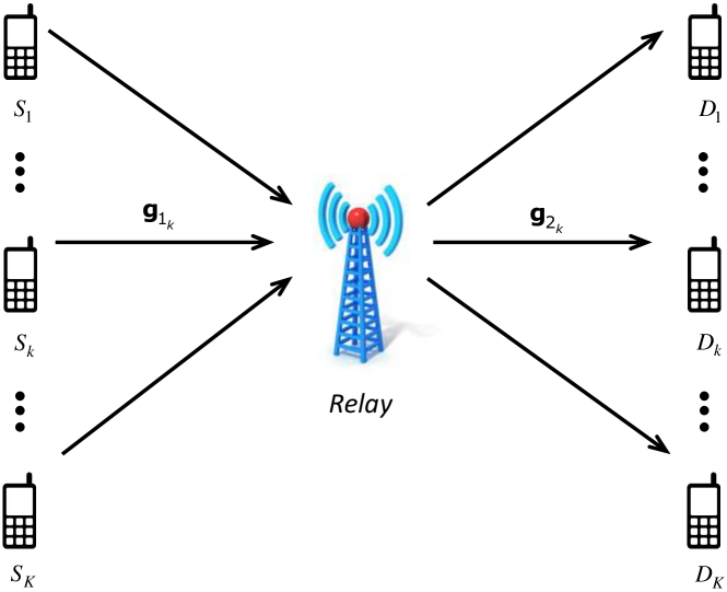
Figure 1: System model. The channel strengths of the source-relay, (${S}_{k}-{R}$) and relay-destination, (${R}-{D}_{k}$) links for $k=1,\ldots,K$ are $\eta_{1k}$ and $\eta_{2k}$, respectively.

II System Model

Consider a scenario with a group of $K$ sources, ${S}_{k}$, $K$ destinations, ${D}_{k}$, for $k=1,\dots,K$, and a single relay, ${R}$. Each source/destination is equipped with a single antenna while ${R}$ is equipped with $N$ antennas as shown in Fig. 1. The source ${S}_{k}$ wants to communicate with the destination ${D}_{k}$. Communication in this network occurs via ${R}$ since there are no direct links among ${S}_{k}$ and ${D}_{k}$, for any $k$ due to heavy shadowing and path loss phenomenon.

During the first phase all sources simultaneously transmit their symbols to ${R}$, and the received $N\times 1$ signal vector can be written as

$${\boldsymbol{y}}_{{R}}=\sqrt{P_{\mathsf{t}}}{\boldsymbol{G}}_{1}{\boldsymbol{x}}+{\boldsymbol{n}}_{{R}},$$ (1)

where $\sqrt{P_{\mathsf{t}}}{\boldsymbol{x}}=\sqrt{P_{\mathsf{t}}}[x_{1},x_{2},\dots,x_{K}]^{T}$ are transmitted symbols with $\operatorname{\mathbb{E}}\{{\boldsymbol{x}}{\boldsymbol{x}}^{\dagger}\}={\boldsymbol{I}}_{K}$ (the average transmitted power of each source is $P_{\mathsf{t}}$) and ${\boldsymbol{n}}_{{R}}$ is an $N\times 1$ additive white Gaussian noise (AWGN) vector at the relay node with $\operatorname{\mathbb{E}}\{{\boldsymbol{n}}_{{R}}{\boldsymbol{n}}_{{R}}^{\dagger}\}=\sigma^{2}_{n}{\boldsymbol{I}}_{N}$. The $N\times K$ channel matrix between the $K$ sources and ${R}$ is expressed as ${\boldsymbol{G}}_{1}={\boldsymbol{H}}_{1}{\boldsymbol{D}}_{1}^{1/2}$ where ${\boldsymbol{H}}_{1}$ contains independent and identically distributed (i.i.d.) $\mathcal{CN}\left({0},{1}\right)$ entries and ${\boldsymbol{D}}_{1}$ is a $K\times K$ diagonal matrix, where $[{\boldsymbol{D}}_{1}]_{kk}=\eta_{1k}$. Moreover, we model the $N\times K$ channel matrix between the $K$ destinations and ${R}$ as ${\boldsymbol{G}}_{2}={\boldsymbol{H}}_{2}{\boldsymbol{D}}_{2}^{1/2}$ where ${\boldsymbol{H}}_{2}$ contains i.i.d. $\mathcal{CN}\left({0},{1}\right)$ entries and ${\boldsymbol{D}}_{2}$ is a $K\times K$ diagonal matrix, where $[{\boldsymbol{D}}_{2}]_{kk}=\eta_{2k}$. Note that ${\boldsymbol{H}}_{1}$ and ${\boldsymbol{H}}_{2}$ represent independent fast fading, while ${\boldsymbol{D}}_{1}$ and ${\boldsymbol{D}}_{2}$ represent path-loss attenuation, and log-normal shadow fading. The assumption of independent fast fading is sufficiently realistic for systems where the antennas are spaced sufficiently far apart [5].

During the second phase, ${R}$ re-transmits a transformation of the received signal given by $\widetilde{{\boldsymbol{y}}}_{R}={\boldsymbol{W}}{\boldsymbol{y}}_{{R}}$. The signal at ${D}_{k}$ can be expressed as

$$y_{{D}_{k}}=\sqrt{P_{\mathsf{t}}}{\boldsymbol{g}}_{2_{k}}^{{\dagger}}{\boldsymbol{W}}{\boldsymbol{g}}_{1_{k}}x_{k} +\sqrt{P_{\mathsf{t}}}\sum_{i=1,i\neq k}^{K}{\boldsymbol{g}}_{2_{k}}^{{\dagger}}{\boldsymbol{W}}{\boldsymbol{g}}_{1_{i}}x_{i}$$

$$+{\boldsymbol{g}}_{2_{k}}^{{\dagger}}{\boldsymbol{W}}{\boldsymbol{n}}_{{R}}+n_{{D}_{k}},$$ (2)

where ${\boldsymbol{g}}_{1_{i}}$ is the $i$-th column of ${\boldsymbol{G}}_{1}$, ${\boldsymbol{g}}_{2_{k}}$ is the $k$-th column of ${\boldsymbol{G}}_{2}$, ${\boldsymbol{W}}$ is the $N\times N$ transformation matrix normalized to satisfy a total power constraint, $P_{\mathsf{r}}$, at the relay as $\mathsf{Tr}\left(\mathtt{E}\left\{\widetilde{{\boldsymbol{y}}}_{R}\widetilde{{\boldsymbol{y}}}_{R}^{{\dagger}}\right\}\right)=P_{\mathsf{r}}$, and $n_{{D}_{k}}$ is the AWGN at ${D}_{k}$ with $\mathtt{E}\{n_{{D}_{k}}n_{{D}_{k}}^{\dagger}\}=\sigma^{2}_{n}$.

As a result, the instantaneous end-to-end (e2e) signal-to-interference-noise ratio (SINR) at ${D}_{k}$ can be written as

$$\gamma_{k}=\frac{P_{\mathsf{t}}|{\boldsymbol{g}}_{2_{k}}^{{\dagger}}{\boldsymbol{W}}{\boldsymbol{g}}_{1_{k}}|^{2}}{P_{\mathsf{t}}\sum\limits_{i=1,i\neq k}^{K}|{\boldsymbol{g}}_{2_{k}}^{{\dagger}}{\boldsymbol{W}}{\boldsymbol{g}}_{1_{i}}|^{2}+\|{\boldsymbol{g}}_{2_{k}}^{{\dagger}}{\boldsymbol{W}}\|^{2}\sigma^{2}_{n}+\sigma^{2}_{n}}.$$ (3)

II-A MRC/MRT at the Relay

When CSI is available at ${R}$, it is natural to apply a transformation based on the MRC/MRT principle. In the first phase, the relay uses MRC to combine the signals transmitted from $K$ sources and then in the second phase, it uses MRT precoding to forward data to $K$ destinations. Hence the relay transformation matrix is given by ${\boldsymbol{W}}=a_{\mathsf{mrc}}{\boldsymbol{G}}_{2}{\boldsymbol{G}}_{1}^{{\dagger}}$. In this case, to meet the power constraint at the relay, we have

$$a_{\mathsf{mrc}}=\sqrt{\frac{P_{\mathsf{r}}}{\mathsf{Tr}\left(P_{\mathsf{t}}\left({\boldsymbol{G}}_{1}^{\dagger}{\boldsymbol{G}}_{1}\right)^{2}{\boldsymbol{G}}_{2}^{{\dagger}}{\boldsymbol{G}}_{2}+\sigma^{2}_{n}{\boldsymbol{G}}_{1}^{{\dagger}}{\boldsymbol{G}}_{1}{\boldsymbol{G}}_{2}^{{\dagger}}{\boldsymbol{G}}_{2}\right)}}.$$ (4)

From (II), the received signal at ${D}_{k}$ for MRC/MRT at the relay is given by

$$y_{{D}_{k}}\!\!=\!a_{\mathsf{mrc}}\sqrt{P_{\mathsf{t}}}{\boldsymbol{g}}_{2_{k}}^{{\dagger}}{\boldsymbol{G}}_{2}{\boldsymbol{G}}_{1}^{\dagger}{\boldsymbol{g}}_{1_{k}}x_{k} \!+\!a_{\mathsf{mrc}}\sqrt{P_{\mathsf{t}}}\!\!\!\!\sum_{i=1,i\neq k}^{K}\!\!\!{\boldsymbol{g}}_{2_{k}}^{{\dagger}}{\boldsymbol{G}}_{2}{\boldsymbol{G}}_{1}^{\dagger}{\boldsymbol{g}}_{1_{i}}x_{i}$$

$$+a_{\mathsf{mrc}}{\boldsymbol{g}}_{2_{k}}^{{\dagger}}{\boldsymbol{G}}_{2}{\boldsymbol{G}}_{1}^{\dagger}{\boldsymbol{n}}_{{R}}+n_{{D}_{k}}.$$ (5)

Hence, the e2e SINR can be expressed as

$$\gamma^{\mathsf{mrc}}_{k}=\frac{P_{\mathsf{t}}\frac{|{\boldsymbol{g}}_{2_{k}}^{{\dagger}}{\boldsymbol{G}}_{2}{\boldsymbol{G}}_{1}^{{\dagger}}{\boldsymbol{g}}_{1_{k}}|^{2}}{\|{\boldsymbol{g}}_{2_{k}}^{{\dagger}}{\boldsymbol{G}}_{2}{\boldsymbol{G}}_{1}^{{\dagger}}\|^{2}}}{P_{\mathsf{t}}\sum\limits_{i=1,i\neq k}^{K}\frac{|{\boldsymbol{g}}_{2_{k}}^{{\dagger}}{\boldsymbol{G}}_{2}{\boldsymbol{G}}_{1}^{{\dagger}}{\boldsymbol{g}}_{1_{i}}|^{2}}{\|{\boldsymbol{g}}_{2_{k}}^{{\dagger}}{\boldsymbol{G}}_{2}{\boldsymbol{G}}_{1}^{{\dagger}}\|^{2}}+\sigma^{2}_{n}+\frac{\sigma^{2}_{n}}{a_{\mathsf{mrc}}^{2}\|{\boldsymbol{g}}_{2_{k}}^{{\dagger}}{\boldsymbol{G}}_{2}{\boldsymbol{G}}_{1}^{{\dagger}}\|^{2}}}.$$ (6)

II-B ZF at the Relay

We now consider the use of ZF receivers and precoders at the relay. With ZF processing, the transformation matrix can be expressed as ${\boldsymbol{W}}=a_{\mathsf{zf}}{\boldsymbol{G}}_{2}\left({\boldsymbol{G}}_{2}^{{\dagger}}{\boldsymbol{G}}_{2}\right)^{-1}\left({\boldsymbol{G}}_{1}^{{\dagger}}{\boldsymbol{G}}_{1}\right)^{-1}{\boldsymbol{G}}_{1}^{{\dagger}}$, where $a_{\mathsf{zf}}$ is chosen to satisfy the power constraint at the relay, i.e.,

$$a_{\mathsf{zf}}=\sqrt{\frac{P_{\mathsf{r}}}{\mathsf{Tr}\left(P_{\mathsf{t}}\left({\boldsymbol{G}}_{2}^{\dagger}{\boldsymbol{G}}_{2}\right)^{-1}+\sigma^{2}_{n}\left({\boldsymbol{G}}_{2}^{\dagger}{\boldsymbol{G}}_{2}\right)^{-1}\left({\boldsymbol{G}}_{1}^{\dagger}{\boldsymbol{G}}_{1}\right)^{-1}\right)}}.$$ (7)

For this case, we have

$${\boldsymbol{g}}_{2_{k}}^{{\dagger}}{\boldsymbol{W}}{\boldsymbol{g}}_{1_{i}}=a_{\mathsf{zf}}\delta_{ki},$$ (8)

where $\delta_{ki}=1$ when $k=i$ and $0$ otherwise. Therefore, from (II), we can write the received signal at $D_{k}$ as

$$y_{D_{k}}=a_{\mathsf{zf}}\sqrt{P_{\mathsf{t}}}x_{k}+a_{\mathsf{zf}}\left[\left({\boldsymbol{G}}_{1}^{{\dagger}}{\boldsymbol{G}}_{1}\right)^{-1}{\boldsymbol{G}}_{1}^{{\dagger}}\right]_{{k}}{\boldsymbol{n}}_{{R}}+n_{D_{k}},$$ (9)

where $\left[{\boldsymbol{A}}\right]_{k}$ is the $k$-th row of the matrix ${\boldsymbol{A}}$.

Now we can express the e2e signal-to-noise ratio (SNR) as

$$\gamma^{\mathsf{zf}}_{k}=\frac{a^{2}_{\mathsf{zf}}P_{\mathsf{t}}}{a^{2}_{\mathsf{zf}}\left[\left({\boldsymbol{G}}_{1}^{{\dagger}}{\boldsymbol{G}}_{1}\right)^{-1}\right]_{{kk}}\sigma^{2}_{n}+\sigma^{2}_{n}}.$$ (10)

II-C Orthogonal Scheme

For comparison with MRC/MRT and ZF, we also consider a “naive scheme” that employs orthogonal channel access. Specifically, to completely avoid the inter-user interference, each $S_{k}-D_{k}$ pair for $k=1,\ldots,K$ uses $\frac{1}{2K}$ channel resources for communication. At the relay, MRC/MRT is employed as it maximizes the e2e SNR. Therefore, the e2e SNR at $D_{k}$ can be expressed as

$$\gamma^{\mathsf{ns}}_{k}=\frac{\frac{P_{\mathsf{t}}\|{\boldsymbol{g}}^{{\dagger}}_{1_{k}}\|^{2}}{\sigma^{2}_{n}}\frac{P_{\mathsf{r}}\|{\boldsymbol{g}}_{2_{k}}\|^{2}}{\sigma^{2}_{n}}}{\frac{P_{\mathsf{t}}\|{\boldsymbol{g}}^{{\dagger}}_{1_{k}}\|^{2}}{\sigma^{2}_{n}}+\frac{P_{\mathsf{r}}\|{\boldsymbol{g}}^{{\dagger}}_{2_{k}}\|^{2}}{\sigma^{2}_{n}}+1}.$$ (11)

III Large $N$ Analysis

In this section, we further simplify the e2e SINR expressions (6) and (10) in the very large $N$ regime. These new expressions illuminate several aspects of the achievable rate vs. power efficiency performance in the considered network. Here we assume that $N\gg K$. We further assume that when $N$ is large, the elements of the channel matrices ${\boldsymbol{G}}_{1}$ and ${\boldsymbol{G}}_{2}$ are still independent. Note that even with very large $N$, the physical size of the antenna array can be small. For example, at $2.6$ GHz, a cylindrical array with $128$ antennas and $\lambda/2$ antenna spacing occupies only a physical size of $28~{}\text{cm}\times 29$ cm and even with this array, the antennas experience nearly independent fading [3, 14].

The achievable ergodic sum rate of the system is given by

$$C_{\mathsf{sum}}^{\star}=\operatorname{\mathbb{E}}\left\{\sum^{K}_{k=1}\frac{1}{2\alpha_{\mathsf{f}}}\log_{2}\left(1+\gamma^{\star}_{k}\right)\right\},$$ (12)

where $\star=\{\mathsf{mrc},\mathsf{zf},\mathsf{ns}\}$ refers to MRC/MRT, ZF and naive schemes and the pre-log factor $\frac{1}{2}$ is due to the half-duplex relaying. For MRC/MRT and ZF: $\alpha_{\mathsf{f}}=1$ and for the naive scheme $\alpha_{\mathsf{f}}=K$.

In the following analysis, we will consider three cases: namely, Case I) Fixed $NP_{\mathsf{t}},N\rightarrow\infty$; Case II) Fixed $NP_{\mathsf{r}},N\rightarrow\infty$; Case III) Fixed $NP_{\mathsf{t}}$, Fixed $NP_{\mathsf{r}},N\rightarrow\infty$.

III-A MRC/MRT at the Relay

Case I): If $P_{\mathsf{t}}=\frac{E_{\mathsf{t}}}{N}$ where $E_{\mathsf{t}}$ is fixed, then from (II-A) we have

$$\frac{y_{{D}_{k}}}{\sqrt{N}} \!=\!\frac{a_{\mathsf{mrc}}\sqrt{E_{\mathsf{t}}}{\boldsymbol{g}}^{{\dagger}}_{2_{k}}{\boldsymbol{G}}_{2}{\boldsymbol{G}}_{1}^{{\dagger}}{\boldsymbol{g}}_{1_{k}}x_{k}}{N}+\!\!\!\!\!\!\!\sum^{K}_{i=1,i\neq k}\!\!\!\!\!\frac{a_{\mathsf{mrc}}\sqrt{E_{\mathsf{t}}}{\boldsymbol{g}}^{{\dagger}}_{2_{k}}{\boldsymbol{G}}_{2}{\boldsymbol{G}}_{1}^{{\dagger}}{\boldsymbol{g}}_{1_{i}}x_{i}}{N}$$

$$+\frac{a_{\mathsf{mrc}}{\boldsymbol{g}}^{{\dagger}}_{2_{k}}{\boldsymbol{G}}_{2}{\boldsymbol{G}}_{1}^{{\dagger}}{\boldsymbol{n}}_{{R}}}{\sqrt{N}}+\frac{n_{{D}_{k}}}{\sqrt{N}}.$$ (13)

In the very large $N$ regime, we apply the law of large numbers given by [15]

$$\frac{{\boldsymbol{g}}^{{\dagger}}_{2_{k}}{\boldsymbol{g}}_{2_{i}}}{N}\mathop{\to}\limits^{a.s.}_{N\to\infty}\left\{\begin{array}[]{l l}0&\quad i\neq k\\ 1&\quad i=k\\ \end{array}\right.$$ (16)

and note that

$$Na_{\mathsf{mrc}} =\sqrt{\frac{P_{\mathsf{r}}}{\mathsf{Tr}\left(\frac{E_{\mathsf{t}}}{N^{3}}\left({\boldsymbol{G}}_{1}^{\dagger}{\boldsymbol{G}}_{1}\right)^{2}{\boldsymbol{G}}_{2}^{{\dagger}}{\boldsymbol{G}}_{2}+\sigma^{2}_{n}\frac{1}{N^{2}}{\boldsymbol{G}}_{1}^{{\dagger}}{\boldsymbol{G}}_{1}{\boldsymbol{G}}_{2}^{{\dagger}}{\boldsymbol{G}}_{2}\right)}}$$

$$\mathop{\to}\limits^{a.s.}_{N\to\infty}\sqrt{\frac{P_{\mathsf{r}}}{\mathsf{Tr}\left(E_{\mathsf{t}}{\boldsymbol{D}}_{1}^{2}{\boldsymbol{D}}_{2}+\sigma^{2}_{n}{\boldsymbol{D}}_{1}{\boldsymbol{D}}_{2}\right)}}.$$ (17)

Now re-expressing the first term in (III-A) as

$$a_{\mathsf{mrc}}\sqrt{E_{\mathsf{t}}}\>\frac{{\boldsymbol{g}}^{{\dagger}}_{2_{k}}{\boldsymbol{G}}_{2}{\boldsymbol{G}}_{1}^{{\dagger}}{\boldsymbol{g}}_{1_{k}}}{N}=Na_{\mathsf{mrc}}\sqrt{E_{\mathsf{t}}}\sum^{K}_{i=1}\frac{{\boldsymbol{g}}^{{\dagger}}_{2_{k}}{\boldsymbol{g}}_{2_{k}}{\boldsymbol{g}}^{{\dagger}}_{1_{k}}{\boldsymbol{g}}_{1_{k}}}{N^{2}}.$$

Therefore, when $N$ tends to infinity, we have

$$a_{\mathsf{mrc}}\sqrt{E_{\mathsf{t}}}\>\frac{{\boldsymbol{g}}^{{\dagger}}_{2_{k}}{\boldsymbol{G}}_{2}{\boldsymbol{G}}_{1}^{{\dagger}}{\boldsymbol{g}}_{1_{k}}}{N}\mathop{\to}\limits^{a.s.}\sqrt{\!\!\frac{P_{\mathsf{r}}E_{\mathsf{t}}}{\mathsf{Tr}\!\left(\!E_{\mathsf{t}}{\boldsymbol{D}}_{1}^{2}{\boldsymbol{D}}_{2}\!+\!\sigma^{2}_{n}{\boldsymbol{D}}_{1}{\boldsymbol{D}}_{2}\!\right)}}\eta_{1k}\eta_{2k}.$$ (18)

Similarly, for $i\neq k$, re-expressing the second term in (III-A) as

$$a_{\mathsf{mrc}}\sqrt{E_{\mathsf{t}}}\>\frac{{\boldsymbol{g}}^{{\dagger}}_{2_{k}}{\boldsymbol{G}}_{2}{\boldsymbol{G}}_{1}^{{\dagger}}{\boldsymbol{g}}_{1_{i}}}{N}=Na_{\mathsf{mrc}}\sqrt{E_{\mathsf{t}}}\sum^{K}_{j=1}\frac{{\boldsymbol{g}}^{{\dagger}}_{2_{k}}{\boldsymbol{g}}_{2_{j}}{\boldsymbol{g}}_{1_{j}}^{{\dagger}}{\boldsymbol{g}}_{1_{i}}}{N^{2}},$$

we obtain

$$a\sqrt{E_{\mathsf{t}}}\>\frac{{\boldsymbol{g}}^{{\dagger}}_{2_{k}}{\boldsymbol{G}}_{2}{\boldsymbol{G}}_{1}^{{\dagger}}{\boldsymbol{g}}_{1_{i}}}{N^{2}}\rightarrow 0.$$ (19)

Note that the third term in (III-A) can be written as

$$a_{\mathsf{mrc}}\frac{{\boldsymbol{g}}^{{\dagger}}_{2_{k}}{\boldsymbol{G}}_{2}{\boldsymbol{G}}_{1}^{{\dagger}}{\boldsymbol{n}}_{{R}}}{\sqrt{N}}=Na_{\mathsf{mrc}}\sum^{K}_{i=1}\frac{{\boldsymbol{g}}^{{\dagger}}_{2_{k}}{\boldsymbol{g}}_{2_{i}}{\boldsymbol{g}}^{{\dagger}}_{1_{i}}{\boldsymbol{n}}_{{R}}}{N\sqrt{N}}.$$

We apply the law of large numbers and the Lindeberg-Lévy central limit theorem and obtain

$$a_{\mathsf{mrc}}\frac{{\boldsymbol{g}}^{{\dagger}}_{2_{k}}{\boldsymbol{G}}_{2}{\boldsymbol{G}}_{1}^{{\dagger}}{\boldsymbol{g}}_{1_{i}}}{\sqrt{N}}\mathop{\to}\limits^{d}\sqrt{\frac{P_{\mathsf{r}}}{\mathsf{Tr}\left(E_{\mathsf{t}}{\boldsymbol{D}}_{1}^{2}{\boldsymbol{D}}_{2}+\sigma^{2}_{n}{\boldsymbol{D}}_{1}{\boldsymbol{D}}_{2}\right)}}\eta_{2k}\widetilde{n}_{R},$$ (20)

where $\widetilde{n}_{R}\sim\mathcal{CN}\left(0,\eta_{1k}\sigma^{2}_{n}\right)$. Substituting (18), (19) and (20) into (III-A) and since $\frac{1}{\sqrt{N}}n_{D_{k}}\rightarrow 0$ we have

$$\frac{y_{{D}_{k}}}{\sqrt{N}} \rightarrow\sqrt{\frac{P_{\mathsf{r}}E_{\mathsf{t}}}{\mathsf{Tr}\left(E_{\mathsf{t}}{\boldsymbol{D}}_{1}^{2}{\boldsymbol{D}}_{2}+\sigma^{2}_{n}{\boldsymbol{D}}_{1}{\boldsymbol{D}}_{2}\right)}}\eta_{1k}\eta_{2k}x_{k}$$

$$+\sqrt{\frac{P_{\mathsf{r}}}{\mathsf{Tr}\left(E_{\mathsf{t}}{\boldsymbol{D}}_{1}^{2}{\boldsymbol{D}}_{2}+\sigma^{2}_{n}{\boldsymbol{D}}_{1}{\boldsymbol{D}}_{2}\right)}}\eta_{2k}\widetilde{n}_{R}.$$ (21)

Now from (III-A) we obtain

$$\gamma^{\mathsf{mrc}}_{k}\rightarrow\frac{E_{\mathsf{t}}\eta_{1k}}{\sigma^{2}_{n}},~{}\text{as}~{}N\to\infty.$$ (22)

For $K=1$, it is clear that we can reduce the transmit power by a factor of $1/N$ with no reduction in performance due to the array gain. But here we consider multiple sources, and the above result implies that by using a large number of relay antennas, we can still obtain the same array gain as in the case of single source. Interestingly, from (22) we can see that when $N$ grows large and $NP_{\mathsf{t}}$ is fixed, the e2e SNR does not depend on the transmit power at the relay and the large-scale fading of the second hop. This is due to the fact that, with MRT precoding at the relay in the second phase and $P_{\mathsf{r}}$ is fixed, as $N$ goes to infinity, the effect of inter-user interference and noise at $D_{k}$ disappears. Finally, the sum rate follows directly by substituting (22) into (12).

Case II): If $P_{\mathsf{r}}=\frac{E_{\mathsf{r}}}{N}$ where $E_{\mathsf{r}}$ is fixed, we observe that

$$N^{2}a_{\mathsf{mrc}} \mathop{\to}\limits^{a.s.}_{N\to\infty}\sqrt{\frac{E_{\mathsf{r}}}{\mathsf{Tr}\left(P_{\mathsf{t}}{\boldsymbol{D}}_{1}^{2}{\boldsymbol{D}}_{2}\right)}}.$$ (23)

Therefore when $N$ grows without bound, the first term in (II-A) tends to

$$a_{\mathsf{mrc}}\sqrt{P_{\mathsf{t}}}{\boldsymbol{g}}^{{\dagger}}_{2_{k}}{\boldsymbol{G}}_{2}{\boldsymbol{G}}_{1}^{{\dagger}}{\boldsymbol{g}}_{1_{k}}\mathop{\to}\limits^{a.s.}\sqrt{\frac{E_{\mathsf{r}}}{\mathsf{Tr}\left({\boldsymbol{D}}_{1}^{2}{\boldsymbol{D}}_{2}\right)}}\eta_{1k}\eta_{2k}.$$ (24)

Similarly, when $N$ goes to infinity, the second and third terms in (II-A) converge almost sure to $0$. Therefore,

$$y_{{D}_{k}} \mathop{\to}\limits^{a.s.}\sqrt{\frac{E_{\mathsf{r}}}{\mathsf{Tr}\left({\boldsymbol{D}}_{1}^{2}{\boldsymbol{D}}_{2}\right)}}\eta_{1k}\eta_{2k}x_{k}+n_{D_{k}},~{}\text{as}~{}N\to\infty.$$ (25)

From (25), as $N\to\infty$, we have

$$\gamma^{\mathsf{mrc}}_{k}\rightarrow\frac{E_{\mathsf{r}}\eta^{2}_{1k}\eta^{2}_{2k}}{\mathsf{Tr}\left({\boldsymbol{D}}_{1}^{2}{\boldsymbol{D}}_{2}\right)\sigma^{2}_{n}}.$$ (26)

The above result shows that the transmit power at relay can be made inversely proportional to the number of relay antennas without compromising the quality-of-service. Note that in the special case where $\eta_{1k}=\eta_{1}$ and $\eta_{2k}=\eta_{2}$ for $k=1,\ldots,K$, we have $\gamma^{\mathsf{mrc}}_{k}\rightarrow\frac{1}{K}\frac{E_{\mathsf{r}}\eta_{2}}{\sigma^{2}_{n}}$ which does not depend on the transmit power of each source and the channel quality of the first hop.

Case III): If $P_{\mathsf{t}}=\frac{E_{\mathsf{t}}}{N}$ and $P_{\mathsf{r}}=\frac{E_{\mathsf{r}}}{N}$ where $E_{\mathsf{t}}$ and $E_{\mathsf{r}}$ are fixed, using a similar approach as above we can show that

$$y_{{D}_{k}} \mathop{\to}\limits^{d}_{n\to\infty}\sqrt{\frac{E_{\mathsf{t}}E_{\mathsf{r}}}{\mathsf{Tr}\left(E_{\mathsf{t}}{\boldsymbol{D}}_{1}^{2}{\boldsymbol{D}}_{2}+\sigma^{2}_{n}{\boldsymbol{D}}_{1}{\boldsymbol{D}}_{2}\right)}}\eta_{1k}\eta_{2k}x_{k}$$

$$+\sqrt{\frac{E_{\mathsf{r}}}{\mathsf{Tr}\left(E_{\mathsf{t}}{\boldsymbol{D}}_{1}^{2}{\boldsymbol{D}}_{2}+\sigma^{2}_{n}{\boldsymbol{D}}_{1}{\boldsymbol{D}}_{2}\right)}}\eta_{2k}\widetilde{n}_{R}+n_{{D}_{k}}.$$ (27)

Therefore,

$$\gamma^{\mathsf{mrc}}_{k}\rightarrow\frac{\frac{E_{\mathsf{t}}\eta_{1k}}{\sigma^{2}_{n}}}{1+\frac{\mathsf{Tr}\left(E_{\mathsf{t}}{\boldsymbol{D}}_{1}^{2}{\boldsymbol{D}}_{2}+\sigma^{2}_{n}{\boldsymbol{D}}_{1}{\boldsymbol{D}}_{2}\right)}{E_{\mathsf{r}}\eta_{1k}\eta^{2}_{2k}}},~{}\text{as}~{}N\to\infty.$$ (28)

Interestingly, by using large antenna arrays, we can scale down both transmit powers of source and relay nodes by a factor of $1/N$ with no reduction in performance. Furthermore, we can see that when $E_{\mathsf{t}}\to\infty$, the above SINR coincides with the result for the case $P_{\mathsf{r}}$ is fixed, and when $E_{\mathsf{r}}\to\infty$, the above SINR coincides with the result for the case $P_{\mathsf{t}}$ is fixed.

In the special case where $\eta_{1k}=\eta_{1}$ and $\eta_{2k}=\eta_{2}$ for $k=1,\ldots,K$; we have $\gamma^{\mathsf{mrc}}_{k}\rightarrow\frac{\frac{E_{\mathsf{t}}\eta_{1}}{\sigma^{2}_{n}}}{1+\frac{K}{\frac{E_{\mathsf{r}}\eta_{2}}{\sigma^{2}_{n}}}\left(1+\frac{E_{\mathsf{t}}\eta_{1}}{\sigma^{2}_{n}}\right)}$.

III-B ZF at the Relay

By following a similar derivation as in the case of MRC/MRT, we can obtain the same power scaling law as follows.

Case I): In the very large $N$ regime we first note that

$$\frac{a_{\mathsf{zf}}}{N}\mathop{\to}\limits^{a.s.}\sqrt{\frac{P_{\mathsf{r}}}{\mathsf{Tr}\left(E_{\mathsf{t}}{\boldsymbol{D}}_{2}^{-1}+\sigma^{2}_{n}\left({\boldsymbol{D}}_{1}{\boldsymbol{D}}_{2}\right)^{-1}\right)}}.$$ (29)

Then from (9) we have

$$\frac{y_{D_{k}}}{\sqrt{N}} \mathop{\to}\limits^{d}_{N\to\infty}\sqrt{\frac{P_{\mathsf{r}}}{\mathsf{Tr}\left(E_{\mathsf{t}}{\boldsymbol{D}}_{2}^{-1}+\sigma^{2}_{n}\left({\boldsymbol{D}}_{1}{\boldsymbol{D}}_{2}\right)^{-1}\right)}}x_{k}$$

$$+\sqrt{\frac{P_{\mathsf{r}}}{\mathsf{Tr}\left(E_{\mathsf{t}}{\boldsymbol{D}}_{2}^{-1}+\sigma^{2}_{n}\left({\boldsymbol{D}}_{1}{\boldsymbol{D}}_{2}\right)^{-1}\right)\eta^{2}_{1k}}}\widetilde{n}_{R}+\frac{n_{D_{k}}}{\sqrt{N}},$$ (30)

where $\widetilde{n}_{R}\sim\mathcal{CN}\left(0,\eta_{1k}\sigma^{2}_{n}\right)$. Hence, when $N$ grows without bound, we obtain

$$\gamma^{\mathsf{zf}}_{k}\mathop{\to}\limits^{a.s.}\frac{E_{\mathsf{t}}\eta_{1k}}{\sigma^{2}_{n}}.$$ (31)

Case II): In this case for very large $N$, $a_{\mathsf{zf}}$ tends to

$$a_{\mathsf{zf}}\mathop{\to}\limits^{a.s.}\sqrt{\frac{E_{\mathsf{r}}}{\mathsf{Tr}\left(P_{\mathsf{t}}{\boldsymbol{D}}_{2}^{-1}\right)}}.$$ (32)

Therefore, we can write (9) as

$$y_{D_{k}} \rightarrow\sqrt{\frac{E_{\mathsf{r}}}{\mathsf{Tr}\left(P_{\mathsf{t}}{\boldsymbol{D}}_{2}^{-1}\right)}}\sqrt{P_{\mathsf{t}}}x_{k}+n_{D_{k}},~{}\text{as}~{}N\to\infty.$$ (33)

which leads to

$$\gamma^{\mathsf{zf}}_{k}\rightarrow\frac{E_{\mathsf{r}}}{\mathsf{Tr}\left({\boldsymbol{D}}_{2}^{-1}\right)\sigma^{2}_{n}},~{}\text{as}~{}N\to\infty.$$ (34)

In the special case when $\eta_{2k}=\eta_{2}$ for $k=1,\ldots,K$, we have $\gamma_{k}\rightarrow\frac{1}{K}\frac{E_{\mathsf{r}}\eta_{2}}{\sigma^{2}_{n}}$.

Case III): If $P_{\mathsf{t}}=\frac{E_{\mathsf{t}}}{N}$ and $P_{\mathsf{r}}=\frac{E_{\mathsf{r}}}{N}$ where $E_{\mathsf{t}}$ and $E_{\mathsf{r}}$ are fixed, when $N$ tends to infinity, we obtain

$$\frac{a_{\mathsf{zf}}}{\sqrt{N}}\mathop{\to}\limits^{a.s.}\sqrt{\frac{E_{\mathsf{r}}}{\mathsf{Tr}\left(E_{\mathsf{t}}{\boldsymbol{D}}_{2}^{-1}+\sigma^{2}_{n}\left({\boldsymbol{D}}_{1}{\boldsymbol{D}}_{2}\right)^{-1}\right)}}.$$ (35)

Therefore,

$$y_{D_{k}} \mathop{\to}\limits^{d}\sqrt{\frac{E_{\mathsf{t}}E_{\mathsf{r}}}{\mathsf{Tr}\left(E_{\mathsf{t}}{\boldsymbol{D}}_{2}^{-1}+\sigma^{2}_{n}\left({\boldsymbol{D}}_{1}{\boldsymbol{D}}_{2}\right)^{-1}\right)}}x_{k}$$ (36)

$$+\sqrt{\frac{E_{\mathsf{r}}}{\mathsf{Tr}\left(E_{\mathsf{t}}{\boldsymbol{D}}_{2}^{-1}+\sigma^{2}_{n}\left({\boldsymbol{D}}_{1}{\boldsymbol{D}}_{2}\right)^{-1}\right)\eta^{2}_{1k}}}\widetilde{n}_{R}+n_{D_{k}},$$

where $\widetilde{n}_{R}\sim\mathcal{CN}\left(0,\eta_{1k}\sigma^{2}_{n}\right)$. Hence, when $N$ goes to infinity, we obtain

$$\gamma^{\mathsf{zf}}_{k}\rightarrow\frac{\frac{E_{\mathsf{t}}\eta_{1k}}{\sigma^{2}_{n}}}{1+\frac{\mathsf{Tr}\left(E_{\mathsf{t}}{\boldsymbol{D}}_{2}^{-1}+\sigma^{2}_{n}\left({\boldsymbol{D}}_{1}{\boldsymbol{D}}_{2}\right)^{-1}\right)\eta_{1k}}{E_{\mathsf{r}}}}.$$ (37)

In the special case where $\eta_{1k}=\eta_{1}$ and $\eta_{2k}=\eta_{2}$ for $k=1,\ldots,K$, we have $\gamma^{\mathsf{zf}}_{k}\rightarrow\frac{\frac{E_{\mathsf{t}}\eta_{1}}{\sigma^{2}_{n}}}{1+\frac{K}{\frac{E_{\mathsf{r}}\eta_{2}}{\sigma^{2}_{n}}}\left(1+\frac{E_{\mathsf{t}}\eta_{1}}{\sigma^{2}_{n}}\right)}$.

Remark 1: In Case I) the asymptotic rate $(N\rightarrow\infty)$ of $D_{k}$ with MRC/MRT and ZF processing is same and given by $C^{\mathsf{mrc}}_{k}=C^{\mathsf{zf}}_{k}=\frac{1}{2}\log_{2}\left(1+\frac{E_{\mathsf{t}}\eta_{1k}}{\sigma^{2}_{n}}\right)$.

Remark 2: In Case II) the asymptotic rates at $D_{k}$ with MRC/MRT and ZF, $C^{\mathsf{mrc}}_{k}\lesseqgtr C^{\mathsf{zf}}_{k}$, is determined by

$$\frac{1}{\eta^{2}_{1k}\eta^{2}_{2k}}\sum^{K}_{i\neq k}\eta^{2}_{1i}\eta_{2i}\gtreqless\sum^{K}_{i\neq k}\frac{1}{\eta_{2i}}.$$ (38)

Remark 3: In Case III) the asymptotic rates at the $k$th destination with MRC/MRT and ZF, $C^{\mathsf{mrc}}_{k}\lesseqgtr C^{\mathsf{zf}}_{k}$, is determined by

$$\frac{1}{\eta^{2}_{1k}\eta^{2}_{2k}}\sum^{K}_{i\neq k}\eta_{1i}\eta_{2i}\left(1+\frac{E_{\mathsf{t}}\eta_{1i}}{\sigma^{2}_{n}}\right)\gtreqless\sum^{K}_{i\neq k}\frac{1}{\eta_{1i}\eta_{2i}}\left(1+\frac{E_{\mathsf{t}}\eta_{1i}}{\sigma^{2}_{n}}\right).$$ (39)

III-C Orthogonal Scheme

We now consider the asymptotic sum rate of the orthogonal scheme. In Case I): It is easy to show that $\gamma^{\mathsf{ns}}_{k}\rightarrow\frac{E_{\mathsf{t}}\eta_{1k}}{\sigma^{2}_{n}}$ and $C^{\mathsf{ns}}_{\mathsf{sum}}=\frac{1}{2K}\sum^{K}_{i=1}\log_{2}\left(1+\frac{E_{\mathsf{t}}\eta_{1k}}{\sigma^{2}_{n}}\right)$. In Case II): $\gamma^{\mathsf{ns}}_{k}\rightarrow\frac{E_{\mathsf{r}}\eta_{2k}}{\sigma^{2}_{n}}$ and $C^{\mathsf{ns}}_{\mathsf{sum}}=\frac{1}{2K}\sum^{K}_{i=1}\log_{2}\left(1+\frac{E_{\mathsf{r}}\eta_{2k}}{\sigma^{2}_{n}}\right)$ and in Case III): We have $\gamma^{\mathsf{ns}}_{k}\rightarrow\frac{\frac{E_{\mathsf{t}}\eta_{1k}}{\sigma^{2}_{n}}\frac{E_{\mathsf{r}}\eta_{2k}}{\sigma^{2}_{n}}}{\frac{E_{\mathsf{t}}\eta_{1k}}{\sigma^{2}_{n}}+\frac{E_{\mathsf{r}}\eta_{2k}}{\sigma^{2}_{n}}+1}$ and

$$C^{\mathsf{ns}}_{\mathsf{sum}}=\frac{1}{2K}\sum^{K}_{i=1}\log_{2}\left(1+\frac{\frac{E_{\mathsf{t}}\eta_{1k}}{\sigma^{2}_{n}}\frac{E_{\mathsf{r}}\eta_{2k}}{\sigma^{2}_{n}}}{\frac{E_{\mathsf{t}}\eta_{1k}}{\sigma^{2}_{n}}+\frac{E_{\mathsf{r}}\eta_{2k}}{\sigma^{2}_{n}}+1}\right).$$ (40)

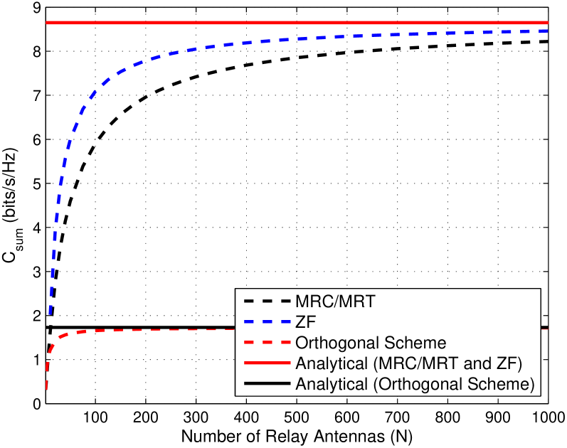
Figure 2: Case I): Sum rate vs. the number of relay antennas. $E_{\mathsf{t}}=10$ dB, $P_{\mathsf{r}}=1$ and $K=5$ users are served. ${\boldsymbol{D}}_{1}={\boldsymbol{D}}_{2}={\boldsymbol{I}}_{5}$.

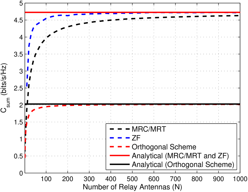
Figure 3: Case II): Sum rate vs. the number of relay antennas. $P_{\mathsf{t}}=1,E_{\mathsf{r}}=10$ dB and $K=5$ users are served. ${\boldsymbol{D}}_{1}={\boldsymbol{D}}_{2}={\boldsymbol{I}}_{5}$.

IV Numerical Results

The sum rates achieved by the multi-pair relay system are evaluated through simulations and compared with our asymptotic analytical results. Without loss of generality, $\sigma^{2}_{n}=1$ is assumed.

Fig. 2 shows the simulated sum rate vs. the number of relay antennas and the presented analytical asymptotic results for Case I). Clearly, as the number of antennas increases, the sum rates of MRC/MRC, ZF and the naive schemes approaches the corresponding constant values predicted by our analysis. Interestingly, the sum rate curve of ZF has a sharper knee than the MRC/MRT counterpart on the way to the same asymptotic constant and the achieved sum rate is $8.65$ bits/s/Hz. Though it is not explicitly seen in Fig. 2, for small number of antennas ($N\leq 6$), the naive scheme exhibits a better sum rate than MRC/MRT as expected. However, as $N$ increases, the sum rate offered by the naive scheme rapidly saturates while the sum rates of the MRC/MRT and ZF schemes show a rapid improvement. This is because with a limited number of antennas, interference cannot be significantly reduced and thus lowers the sum rate of MRC/MRT. But when $N$ grows large, the random channel vectors between sources/destinations and relay become pairwise orthogonal and hence, the interference is canceled out. At the same time, we gain from simultaneously serving $K$ source-destination pairs in the same time-frequency resource.

Figs. 3 and 4 show results for the second and third power scaling laws; Case II) and Case III). Both MRC/MRT and ZF achieves the same sum rate of $4.73$ and $3.36$ bits/s/Hz in Case II) and Case III), respectively. Moreover, similar trends in results as in Fig. 2 can be observed.

The rates achieved by individual destinations are illustrated in Fig. 5 for slow-fading coefficients; $\eta_{11}=2,\eta_{12}=2,\eta_{13}=2$ and $\eta_{21}=1,\eta_{22}=3,\eta_{23}=3$ and Case II). Results in Fig. 5 confirm that the sum rate of MRC/MRT can be higher than the sum rate of ZF depending on the slow fading parameters. $C^{\mathsf{mrc}}_{\mathsf{sum}}=8.98$ and $C^{\mathsf{zf}}_{\mathsf{sum}}=8.90$. Recall that $C^{\mathsf{mrc}}_{\mathsf{sum}}<C^{\mathsf{zf}}_{\mathsf{sum}}$ in the example of Fig. 3. Interestingly, when $N\leq 350$, all three users in the ZF system achieve a higher rate than the users in the MRC system. However, when $N$ is very large, two users of the MRC achieve a higher rate than the ZF users.

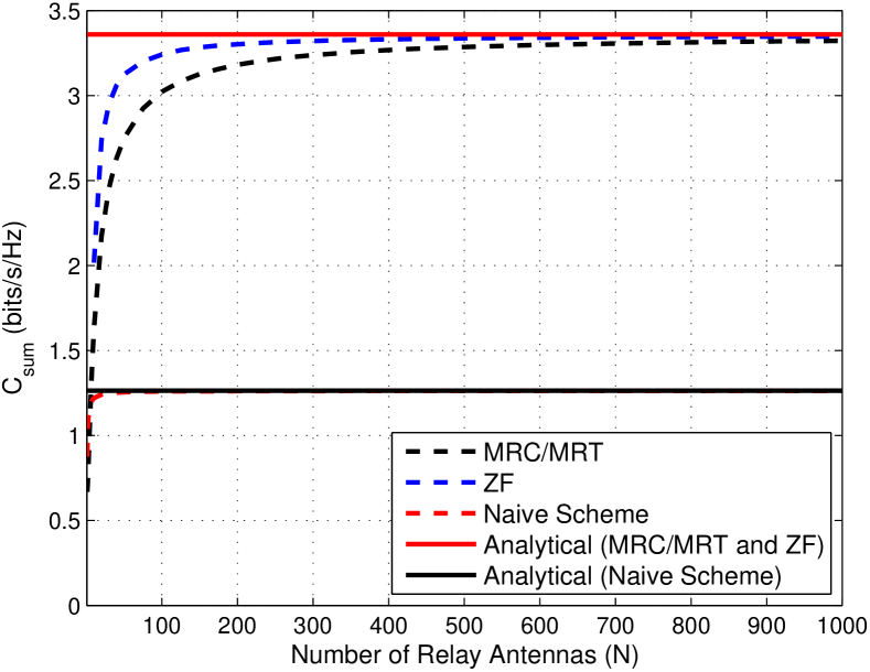
Figure 4: Case III): Sum rate vs. the number of relay antennas. $P_{\mathsf{t}}=10$ dB, $E_{\mathsf{r}}=10$ dB and $K=5$ users are served. ${\boldsymbol{D}}_{1}={\boldsymbol{D}}_{2}={\boldsymbol{I}}_{5}$.

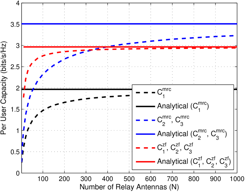
Figure 5: Case II): Per user rate vs. the number of relay antennas. $K=3$ are served.

V Conclusion

We have shown that relay systems can benefit significantly from the use of very large antenna arrays. The offered sum rates of a multi-pair relay system was investigated for three different power scaling laws. At the relay, MRC/MRT and ZF processing was considered. We derived asymptotic sum rate results and confirmed their accuracy using computer simulations. Several insights were extracted using the analysis to illuminate the comparative performances between MRC/MRT and ZF. For example, the asymptotic achievable rates of MRC/MRT and ZF are the same if we scale the power at the sources.

References

- [1] D. Gesbert, M. Kountouris, R. W. Heath Jr., C.-B. Chae, and T. Sälzer, “Shifting the MIMO paradigm,” IEEE Signal Process. Mag., vol. 24, pp. 36–46, Sept. 2007.
- [2] T. L. Marzetta, “Noncooperative cellular wireless with unlimited numbers of base station antennas,” IEEE Trans. Wireless Commun., vol. 9, pp. 3590-3600, Nov. 2010.
- [3] F. Rusek, D. Persson, B. K. Lau, E. G. Larsson, T. L. Marzetta, O. Edfors, and F. Tufvesson, “Scaling up MIMO: Opportunities and challenges with very large arrays,” IEEE Signal Process. Mag., vol. 30, pp. 40-60, Jan. 2013.
- [4] C. Shepard, H. Yu, N. Anand, E. Li, T. Marzetta, Y. R. Yang, and L. Zhong, “Argos: Practical base stations with large-scale multi-user beamforming,” in Proc. ACM MobiCom 2012, Istanbul, Turkey, Aug. 2012, pp. 53-64.
- [5] H. Q. Ngo, E. G. Larsson and T. L. Marzetta, “Energy and spectral efficiency of very large multiuser MIMO systems,” IEEE Trans. Commun., (accepted). [Online]. Available: http://arxiv.org/pdf/1112.3810v2.pdf
- [6] M. Dohler and Y. Li, Cooperative Communications: Hardware, Channel & PHY. Wiley & Sons, 2010.
- [7] A. Agustin and J. Vidal, “Amplify-and-forward cooperation under interference-limited spatial reuse of the relay slot,” IEEE Trans. Wireless Commun., vol. 7, pp. 1952-1962, May 2008.
- [8] N. Yang, M. Elkashlan and J. Yuan, “Outage probability of multiuser relay networks in Nakagami- fading channels,” IEEE Trans. Veh. Technol., vol. 59, pp. 2120-2132, June 2010.
- [9] H. Ding, J. Ge, D. B. da Costa, and Z. Jiang, “A new efficient low-complexity scheme for multi-source multi-relay cooperative networks,” IEEE Trans. Veh. Technol., vol. 60, pp. 716-722, Feb. 2011.
- [10] J. Kim, D. S. Michalopoulos, and R. Schober, “Diversity analysis of multi-user multi-relay networks,” IEEE Trans. Wireless Commun., vol. 10, pp. 2380-2389, July 2011.
- [11] J. Cao, Z. Zhong and F. Wang, “Regenerative multi-way relaying: Relay precoding and ordered MMSE-SIC receiver,” in Proc. IEEE VTC Spring 2012, Yokohama, Japan, May 2012, pp. 1-5.
- [12] Z. Zhao, Z. Ding, M. Peng, W. Wang and K. K. Leung, “A special case of multi-way relay channel: When beamforming is not applicable,” IEEE Trans. Wireless Commun., vol. 10, pp. 2046-2051, July 2011.
- [13] R. H. Y. Louie, Y. Li and B. Vucetic, “Zero forcing in general two-hop relay networks,” in IEEE Trans. Veh. Technol., vol. 59, pp. 191-202, Jan. 2010.
- [14] X. Gao, O. Edfors, F. Rusek, and F. Tufvesson, “Linear pre-coding performance in measured very-large MIMO channels,” in Proc. IEEE VTC Fall 2011, San Francisco, CA, Sept. 2011, pp. 1-5.
- [15] H. Cramér, Random Variables and Probability Distributions, 3rd ed. Cambridge, UK: Cambridge University Press, 1970.