Computing Similarity between a Pair of Trajectories

Abstract

With recent advances in sensing and tracking technology, trajectory data is becoming increasingly pervasive and analysis of trajectory data is becoming exceedingly important. A fundamental problem in analyzing trajectory data is that of identifying common patterns between pairs or among groups of trajectories. In this paper, we consider the problem of identifying similar portions between a pair of trajectories, each observed as a sequence of points sampled from it.

We present new measures of trajectory similarity — both local and global — between a pair of trajectories to distinguish between similar and dissimilar portions. Our model is robust under noise and outliers, it does not make any assumptions on the sampling rates on either trajectory, and it works even if they are partially observed. Additionally, the model also yields a scalar similarity score which can be used to rank multiple pairs of trajectories according to similarity, e.g. in clustering applications. We also present efficient algorithms for computing the similarity under our measures; the worst-case running time is quadratic in the number of sample points.

Finally, we present an extensive experimental study evaluating the effectiveness of our approach on real datasets, comparing with it with earlier approaches, and illustrating many issues that arise in trajectory data. Our experiments show that our approach is highly accurate in distinguishing similar and dissimilar portions as compared to earlier methods even with sparse sampling.

1 Introduction

Trajectories are functions from a time domain—an interval on the real line—to $\mathbb{R}^{d}$ with $d>1$, and observed as sequences of points sampled from them. They arise in the description of any system that evolves over time and are being recorded or inferred from literally hundreds of millions of sensors nowadays, from traffic monitoring systems [26] and recordings of GPS sensors on cell phones [24] to cameras in surveillance systems and those embedded in smart phones, helmets of soldiers in the field [8], medical devices, and scientific experiments and simulations such as molecular dynamic simulations [18].

Taking full advantage of these datasets for creating knowledge and improving our decision making requires availability of effective algorithms and analysis tools for processing, organizing, and querying these trajectory datasets. This step has been lagging behind partly because of huge scale of data, which is constantly growing, but because of other challenges as well. Trajectory datasets are marred by sensing uncertainty, and are heterogeneous in their quality, format, and temporal support. For instance, GPS measurements are only approximately accurate, and the inaccuracy can grow quite large in conditions of poor satellite reception such as urban canyons; many sensors operate on batteries, preferring to send aggregate or approximate measurements to conserve energy (leading to nonuniform and sparse sampling); trajectories retrieved from video typically arrive in bits and pieces. At the same time, individual trajectories can have complex shapes, and even small nuances lead to big differences in their understanding.

A central problem in analyzing trajectory data is to measure similarity between a pair of trajectories and to identify portions that are common between the two trajectories. Besides being interesting in its own right, this problem often lies at the core of classifying, clustering, and computing mean trajectories. In some applications (e.g. handwriting analysis, speech recognition), one of the trajectories is the ground truth and the other is an observed trajectory, while in some other applications (e.g. traffic analysis, video surveillance), both trajectories are observed data.

Problem statement.   Let $P=\langle p_{1},\ldots,p_{m}\rangle$ and $Q=\langle q_{1},\ldots,q_{n}\rangle$ be two sequences of points in $\mathbb{R}^{d}$, sampled from two trajectories $\gamma_{1}$ and $\gamma_{2}$ defined over the time interval $[0,1]$ with added noise. We assume that the trajectories are defined over the same time interval only for the simplicity of presentation; our models and algorithms work even when they are defined over different time intervals. We also assume that $P$ and $Q$ are points sampled from the images of the trajectories and, for simplicity, we ignore the temporal component; again, our models and algorithms work even if we take the temporal component into account.

Ideally, if we knew the two underlying trajectories $\gamma_{1},\gamma_{2}$, then their similar portions can be defined by reparameterizing them using two functions $\alpha:[0,1]\rightarrow\mathbb{R}^{d}$ and $\beta:[0,1]\rightarrow\mathbb{R}^{d}$ and identifying the sub-intervals of $[0,1]$ over which the two of them are similar. However, we only have finite sample points from each trajectory with additional noise, so we identify similar portions between the two by computing correspondences between sample points in one trajectory to points in the other, and vice-versa. Such a set of correspondences must satisfy the following criteria:

1. Similar portions of the trajectories must be identified even if the sampling rates are different. For example, common routes taken by moving objects should be identified even if GPS coordinates are obtained at highly different times.

2. It must take into account noise/outliers, i.e., it must properly discriminate between noise and actual deviations of the two trajectories.

3. It should work even if the trajectories are partially observed, i.e., some portion of a trajectory is missing.

For any given set of correspondences between two trajectories, it is also advantageous to provide a score or measure indicating their degree of similarity. Such a score is not only useful in identifying a good set of correspondences but also as a way to rank multiple pairs of trajectories according to similarity, e.g. in clustering applications.

The objective is to define an appropriate model for correspondences together with an appropriate scoring function to capture the above requirements and given two trajectories, compute correspondences with the optimal score efficient. In addition, we are also interested in identifying most similar contiguous sub-trajectories of two given trajectories. Thus, another objective is to compute local similarity between trajectories.

\begin{picture}(1891.0,2276.0)(8967.0,-8400.0)\end{picture}

Figure 1: A pair of trajectories with small Hausdorff distance but large Fréchet distance.

Related work.   Motivated by a wide range of applications, there is extensive work on computing similarity between two objects (or rather points sampled from the objects) in many fields, including computational geometry, computer vision, computer graphics, and statistical learning. Two of the commonly used methods for measuring similarity are Hausdorff distance [3] and earth-movers distance [22], and their variants. These methods are, however, not suitable for measuring similarity between two trajectories because they only focus on the location of points and not their ordering along the trajectories. A better choice is the so-called Fréchet distance [2] (see Fig. 1). Informally, consider a person and a dog connected by a leash, each walking along a curve from its starting point to its end point. Both are allowed to control their speed, but they cannot backtrack. The Fréchet distance between the two curves is the minimal length of a leash that is sufficient for traversing both curves in this manner. A reparameterization is a continuous non-decreasing surjection $\alpha:[0,1]\rightarrow[0,1]$, such that $\alpha(0)=0$ and $\alpha(1)=1$. The Fréchet distance $\mathop{\mathrm{Fr}}(\gamma_{1},\gamma_{2})$ between two trajectories $\gamma_{1}$ and $\gamma_{2}$ is then defined as follows:

$$\mathop{\mathrm{Fr}}(\gamma_{1},\gamma_{2})=\inf_{\alpha,\beta}\max_{t\in[0,1]}\|\gamma_{1}(\alpha(t))-\gamma_{2}(\beta(t))\|,$$

where $\|\cdot\|$ is the underlying norm (typically, as above, the Euclidean norm), and $\alpha$ and $\beta$ are reparameterizations of $[0,1]$. The Fréchet distance between two polygonal curves with $m$ and $n$ vertices respectively can be computed in $O(mn\log(m+n))$ time [2].

If we only have samples of points on each trajectory, then a simpler variant, called discrete Fréchet distance, is used, where the dog and its owner are replaced by a pair of frogs that can only reside on $n$ and $m$ specific stones $P$ and $Q$ on $\gamma_{1}$ and $\gamma_{2}$, respectively. These frogs hop from one stone to the next without backtracking, and the discrete Fréchet distance is the minimum length of a “leash” that connect the frogs and allows them to execute such a sequence of hops. The discrete Fréchet distance can be computed in $O(mn)$ time by a straightforward quadratic programming algorithm. Recently Agarwal et al. [1] have presented a sub-quadratic algorithm for this problem.

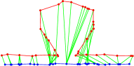
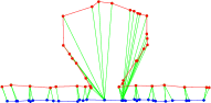
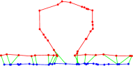
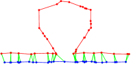
(a)	(b)	(c)	(d)

Figure 2: Computing similarity between two trajectories using different distance measures: (a) Fréchet distance, (b) dynamic time warping or average Fréchet distance, (c) sequence alignment based method, (d) our model.

Although the Fréchet distance is often used as a measure of curve matching, in its traditional definition, an assignment yielding the Fréchet distance is not necessarily a good indicator of the correspondences between the trajectories. The reason for this is because there could possibly exist a large number of correspondences which yield the optimal Fréchet distance since the optimization criteria is the distance between the two farthest points in the coupling; see Fig. 2(a). Thus, in order to identify a good correspondence between the two trajectories, we must resort to the average Fréchet distance, more commonly known as dynamic time warping distance, where we use the analogy of a pair of frogs hopping along $P$ and $Q$, but the goal is to minimize the “average length” of the leash instead of its maximum length. Dynamic time warping (DTW) was originally developed for matching speech signals in speech recognition [21] and computes good correspondences between the two trajectories if they are similar for the most part, as is the case for trajectories corresponding to pairs of speech signals for a word or handwriting trajectories for a particular words or letters.

However, if the trajectories contain significant dissimilar portions, possibly due to actual deviations (such as different routes for GPS trajectories), the results are not as meaningful. Consider Fig. 2(b) which shows two trajectories starting with similar paths but where, one trajectory deviates from the other for a significant portion and then rejoins the original path. DTW tries to find a correspondence for all points and thus, gives correspondences for points in the deviation for which no meaningful one exists. Moreover, the actual measure is skewed by these portions and it is difficult to distinguish them from the similar ones using the obtained correspondences. It is even more difficult to distinguish actual deviations from outliers caused by measurement errors.

There is a rich body of literature on pairwise sequence alignment in computational biology, where the goal is to identify similar portions between two DNA or protein sequences. Given two sequences $A$ and $B$, their alignment is expressed by writing them in two rows respectively such that at each position in the first (resp. second) row, there is either a character in $A$ (resp. $B$) or a blank character (termed as a gap character). Characters in the same column are deemed either identical or similar and characters in a sequence aligned to gap characters do not have a correspondence in the other sequence. A maximal contiguous sequence of gap characters is termed a gap, analogous to our notion of gaps; see Def. 1. The goal is to compute such an alignment which optimizes a similarity scoring function which assigns a score for aligning two characters and a penalty for gaps. The score for an alignment of two characters is an incentive if they are deemed similar and is a penalty if not. See [10, cf. Chapter 2] for further details.

In computational biology, the algorithms for sequence alignments have been extended to aligning two polygonal curves such as protein backbones. We may easily extend this model to the alignment of trajectories with the choice of an appropriate scoring function. We describe such a scoring function in Sec. 2. However, as Fig. 2(c) shows, non-uniform sampling rates cause similar portions to be designated as gaps since correspondences are restricted to be one-to-one.

Various approaches of defining distance in order to distinguish similar and dissimilar portions exist [9] which aim to combine the advantages of DTW as well as sequence alignment. These include the longest common sub-sequence [25], an adaptation of the edit-distance measure [7] for sequences where trajectory points are designated a match if they are closer than a threshold distance and different otherwise, and the Edit-Distance with real penalties measure [6]. The latter tries to incorporate the distances by evaluating dissimilarity of points by their distance to a fixed reference point. However, it is not clear how this point should be chosen and why it is a good indicator of dissimilarity. A drawback of all these measures is that they do not distinguish between noise and actual dissimilarity. In fact, in the application scenarios under consideration in these works, noise is the primary reason for the dissimilarity since the underlying curves are identical unlike the general setting.

Regarding the problem of computing partial or local similarity of curves, Buchin et al. [4] consider the problem of sub-trajectory similarity under a continuous version of the average Fréchet distance where a user-defined parameter specifies the minimum sub-trajectory duration. Further, in [5], the authors show how to compute a “partial” Fréchet distance, i.e., a maximal portion of the trajectory curves which are close enough. However, their algorithm does not work under the Euclidean norm.

Apart from spatial similarity of trajectories, various other patterns have also been considered. In [13, 16], the authors consider various formalizations of interesting patterns such as flock, where a set of trajectories follow each other for a long duration and convergence where a set of trajectories converge at a particular location. In [14, 27], similarity of soccer player trajectories is considered based on significant events such as passing or shooting.

Finally, as mentioned above, computation of similarity is often a requirement for clustering trajectories. We refer to [17, 11, 20] for a few such approaches.

Our contributions.   Our first contribution is the introduction of a new model for correspondences as defined using the notion of assignments in Sec. 2. Together with this model, we design an appropriate way to score assignments which can be used to rank pairs of trajectories according to similarity. The model and scoring function provides a unified framework which encompasses all previous approaches for computing trajectory similarity such as dynamic time warping, sequence alignment, edit-distance and others while satisfying the requirements presented previously in the problem statement. Our model may also be extended to spatio-temporal data by treating time as an extra dimension. For conciseness, we ignore the temporal component in the rest of the paper.

Next, in Sec. 3, we describe a quadratic time dynamic programming based algorithm for computing optimal assignments between two trajectories $P$ and $Q$ under our scoring function. Our algorithm combines ideas from sequence alignment and dynamic time warping and matches the asymptotic running time complexity of these approaches.

In Sec. 4 we show that our model can also be used for performing the so-called local assignment for identifying most similar sub-trajectories between two trajectories $P$ and $Q$. This is done by adapting the model slightly; the algorithm remains the same. Computing local assignments is similar to the notion of local sequence alignment in computational biology.

If the points on $P$ and $Q$ are sampled non-uniformly and at different rates, then mapping each point of $P$ to a point of $Q$ may lead to unnatural alignments. We therefore consider a semi-continuous model in which we interpolate each trajectory between consecutive sampled points, say, by a linear function, and allow a point of $P$ or $Q$ to be assigned to an interpolated point of the other trajectory (cf. Sec. 5). This extension leads to considerably better assignments in cases where sampling rate differences are significant while measurement noise is less significant.

Finally, we show the effectiveness of our model (in Sec. 7) by evaluating it on a number of real datasets and comparing it with sequence alignment, dynamic time warping, and a modified dynamic time warping heuristic to distinguish similar and deviating portions between pairs of trajectories. In practice, our model captures the advantages of both dynamic time warping and sequence-alignment based approaches with none of their drawbacks.

2 Model

Let $P$ and $Q$ be two sequences of points as defined above. We describe our model for measuring similarity between $P$ and $Q$ and finding common portions of them. Our model builds on the strengths of both dynamic time warping (DTW) and sequence alignment. Recall that

• DTW does not handle deviations well because it tries to match every point on $P$ and $Q$, but it can handle non-uniform sampling of points by allowing multiple points of $P$ to match with one point of $Q$, and vice versa; see Fig. 2(b).

• The sequence alignment model identifies deviations well while distinguishing them from noise but does not allow multiple points of $P$ to match with one point of $Q$, and hence, has issues with non-uniform sampling; see Fig. 2(c).

The following notion of assignments models correspondences between $P$ and $Q$ which captures the advantages of the above approaches without their drawbacks. Together with an appropriate scoring function defined later, assignments accurately reflects the degree of similarity of one trajectory to the other by satisfying the requirements posed in the problem statement in Sec. 1.

Definition 1

An assignment for $P$ and $Q$ is a pair of functions $\alpha:P\rightarrow Q\cup\{{\scriptsize\bot}\}$ and $\beta:Q\rightarrow P\cup\{{\scriptsize\bot}\}$ for the points of $P$ and $Q$ respectively. If $\alpha(p_{i})={\scriptsize\bot}$ (or $\beta(q_{j})={\scriptsize\bot}$), then $p_{i}$ (or $q_{j}$) is called a gap point. A maximal contiguous sequence of gap points in $P$ or $Q$ is called a gap.

An assignment is monotone if it satisfies the following conditions: (i) if $\alpha(p_{i})=q_{j}$ then for all $i^{\prime}>i$, $\alpha(p_{i^{\prime}})={\scriptsize\bot}$ or $\alpha(p_{i^{\prime}})=q_{j^{\prime}}$ for some $j^{\prime}>j$, and (ii) if $\beta(q_{j})=p_{i}$ then for all $j^{\prime}>j$, $\beta(q_{j^{\prime}})={\scriptsize\bot}$ or $\beta(q_{j^{\prime}})=p_{i^{\prime}}$ for some $i^{\prime}>i$.

Intuitively, if a point $p_{i}\in P$ lies on a similar portion of the two trajectories then $\alpha(p_{i})$ defines the point on $Q$ to which $p_{i}$ corresponds, and $p_{i}$ is a gap point otherwise. A similar interpretation holds for $\beta(\cdot)$. Unlike traditional alignment/matching models, our assignments are asymmetric which allows it to better adapt to trajectories with different sampling rates. The notion of gaps is introduced to identify deviations between the two trajectories. Using gaps enables the identification of a “good” assignment even if there are only partial observations on any of the trajectories; we can compute an assignment for the observed portions. Distinguishing between noise and dissimilarity can be accomplished by restricting to assignments where gaps are sufficiently long (short deviations are more likely to be due to noise and thus, the underlying portions of the trajectories are similar).

It will be easier to view an assignment of $P$ and $Q$ in terms of the complete directed bipartite graph $G:=G(P,Q)=(P\cup Q,P\times Q\cup Q\times P)$, i.e., $G$ has a directed edge $(p_{i},q_{j})$ and another directed edge $(q_{j},p_{i})$ for every pair $p_{i}\in P$ and $q_{j}\in Q$. We say that a pair of edges $(p_{i},q_{j})$ (or $(q_{j},p_{i})$) and $(p_{k},q_{l})$ (or $(q_{l},p_{k})$) cross if $i<k$ and $j>l$ or vice versa. Under our definition, the opposite edges $(p_{i},q_{j})$ and $(q_{j},p_{i})$ do not cross each other.

Hence, in this perspective, a monotone assignment is a set $E$ of pairwise non-crossing edges in $G$ so that $E$ has at most one outgoing edge from every point in $P\cup Q$. Points with no outgoing edges are gap points and, as in Def. 1, a maximal contiguous sequence of gap points in $P$ or $Q$ is called a gap, and the length of the sequence is called the length of the gap. Let $\Gamma(E)$ denote the set of gaps in $P$ and $Q$ for the assignment $E$. We define the score of $E$, denoted by $\sigma(P,Q;E)$, as

$$\sigma(P,Q;E)=\sum_{(u,v)\in E}\frac{1}{c+\|u-v\|^{2}}+\sum_{g\in\Gamma(E)}a+\Delta|g|,$$ (1)

where $a,\Delta$ and $c$ are parameters which are chosen carefully, as described in Sec. 6, $\|\cdot\|$ is the $L_{2}$-norm and $|g|$ is the length of a gap $g$. For appropriate comparison between different pairs of trajectories and their corresponding assignments, the above score may be normalized in a straightforward manner to provide a score between 0 and 1. We can rewrite the score in terms of the functions $\alpha,\beta$ from Def. 1 as well:

$$\sigma(P,Q;\alpha,\beta)= \sum_{\begin{subarray}{c}p_{i}\in P\\ \alpha(i)\neq{\scriptsize\bot}\end{subarray}}\frac{1}{c+\|p_{i}-\alpha(p_{i})\|^{2}}$$

$$+\sum_{\begin{subarray}{c}q_{j}\in Q\\ \beta(j)\neq{\scriptsize\bot}\end{subarray}}\frac{1}{c+\|q_{j}-\beta(q_{j})\|^{2}}+\sum_{g\in\Gamma(\alpha,\beta)}\Big{(}a+\Delta\cdot|g|\Big{)},$$ (2)

where $\Gamma(\alpha,\beta)$ is the set of gaps in $P$ and $Q$ for the assignment $\alpha,\beta$.

We define the similarity between $P$ and $Q$ as

$$\sigma(P,Q)=\max_{\alpha,\beta}\sigma(P,Q;\alpha,\beta).$$

The assignment $\alpha^{*},\beta^{*}=\operatorname*{arg\,max}_{\alpha,\beta}\sigma(P,Q;\alpha,\beta)$ identifies the similar portions of $P$ and $Q$.

Why the directed graph?   We now explain why we chose a directed graph model and an assignment. Both DTW and sequence alignment can be formulated as computing a subset of non-crossing edges in the complete undirected bipartite graph $P\times Q$. In particular, DTW finds a subset $D\subset P\times Q$ of non-crossing edges such that each vertex of $P\cup Q$ is incident on at least one edge of $D$ and the total “length” of edges in $D$ is minimum. In some applications, an appropriate choice for the length of edges would be the Euclidean distance whereas in other applications, a different function is used. On the other hand, the sequence-alignment model asks for computing a matching $M\subset P\times Q$ whose score is maximum, where the score of a matching is similar to (1).

It is tempting to describe an assignment as well with respect to the undirected graph but this leads to difficulties. For example, we may relax the condition of finding a “matching” from the sequence-alignment model allowing multiple points of $P$ to match with one point of $Q$, (see Fig. 4(a)) and simply ask for finding a set of non-crossing edges whose score is maximum, but this is not always meaningful and introduces additional edges that are redundant. For example, in Fig. 4(b), this approach will find three edges — the diagonal edge $(p_{2},q_{1})$ is spurious and is an artifact of the model because it is more meaningful to match $p_{1}$ with $q_{1}$, $p_{2}$ with $q_{2}$ and vice versa.

The directed graph model avoids this problem by not requiring the functions $\alpha$ and $\beta$ to be symmetric; see Fig. 4.

(a)	(b)

Figure 3: Pros and cons of allowing multiple matches in an undirected graph:(a) A situation where allowing multiple matches is logical. (b) A situation where allowing multiple matches does not allow us to obtain a clear correspondence.

(a)	(b)

Figure 4: Using a directed graph provides a logical set of correspondences always. Comparison with the examples of Fig. 4.

There are a few other subtle advantages of using the directed graph model, omitted from this abstract due to lack of space.

Remark.   (i) Our framework is not limited to the scoring function (1). For example, the sequence-alignment based approach, DTW or other measures such as edit-distance are easily incorporated into our model. (ii) Note that according to our definition of assignments, vertices in $G$ which have incoming edges but no outgoing edges are designated as gap points. This may be easily modified so gap points have no incoming edges.

$$\sigma(i,j)=\max\Big{\{} \sigma_{{\scriptsize\bot},*}(i,j),\sigma_{*,{\scriptsize\bot}}(i,j),\sigma_{\phi,*}(i,j)+\delta(i,j),\sigma_{*,\phi}(i,j)+\delta(i,j)\Big{\}}$$ (3)

$$\sigma_{{\scriptsize\bot},*}(i,j)=\max\Big{\{} \sigma(i-1,j)+a+\Delta,\sigma_{{\scriptsize\bot},*}(i-1,j)+\Delta,\sigma_{{\scriptsize\bot},\phi}(i,j)+\delta(i,j),$$

$$\sigma_{{\scriptsize\bot},{\scriptsize\bot}}(i,j)\Big{\}}$$ (4)

$$\sigma_{\phi,*}(i,j)=\max\Big{\{} \sigma_{\phi,{\scriptsize\bot}}(i-1,j),\sigma_{*,\phi}(i-1,j)+\delta(i,j),\sigma_{\phi,*}(i,j-1)+\delta(i,j),$$

$$\sigma(i-1,j)\Big{\}},$$ (5)

$$\sigma_{\phi,{\scriptsize\bot}}(i,j)=\max\Big{\{} \sigma_{\phi,*}(i,j-1)+a+\Delta,\sigma_{\phi,{\scriptsize\bot}}(i,j-1)+\Delta,\sigma_{*,{\scriptsize\bot}}(i-1,j)\Big{\}},$$ (6)

$$\sigma_{{\scriptsize\bot},{\scriptsize\bot}}(i,j)=\max\Big{\{} \sigma_{*,{\scriptsize\bot}}(i-1,j)+a+\Delta,\sigma_{{\scriptsize\bot},{\scriptsize\bot}}(i-1,j)+\Delta,\sigma_{{\scriptsize\bot},*}(i,j-1)+a+\Delta,$$

$$\sigma_{{\scriptsize\bot},{\scriptsize\bot}}(i,j-1)+\Delta\Big{\}}.$$ (7)

Figure 5: Recurrence relations for $\sigma$ and each of the auxiliary functions. The relations for $\sigma_{*,\phi}$, $\sigma_{{\scriptsize\bot},\phi}$ are symmetric to those above for $\sigma_{\phi,*}$ and $\sigma_{\phi,{\scriptsize\bot}}$ respectively. Here, $\delta(i,j)=1/(c+\|p_{i}-q_{j}\|^{2})$.

3 Algorithms

We now describe an algorithm for computing the optimal score $\sigma(P,Q)$ and the corresponding assignment. Our algorithm is similar to that for sequence alignment [19] and runs in $O(mn)$ time. The main difference is that, because of the asymmetric nature of the definition of assignments, the recurrence relation is more complex and we need to compute a few auxiliary assignments and score functions.

Auxiliary functions.   For $1\leq i\leq m$, let $P_{i}=\langle p_{1},\dots,p_{i}\rangle$ denote the prefix of $P$ of length $i$, and for $1\leq j\leq n$, let $Q_{j}=\langle q_{1},\dots,q_{j}\rangle$ denote the prefix of $Q$ of length $j$. The algorithm computes the similarity score $\sigma(P_{i},Q_{j})$ for all $1\leq i\leq m$ and $1\leq j\leq n$. For brevity, we will use $\sigma(i,j)$ to denote $\sigma(P_{i},Q_{j})$. Let $\Sigma(i,j)$ denote the (optimal) monotone assignment corresponding to the score $\sigma(i,j)$. With a slight abuse of notation, we will use both the graph representation — a set of non-crossing edges — as well as the pair of functions $\alpha,\beta$. It will be clear from the context which of the two representations we are referring to.

For each pair $i,j$, to compute $\sigma(i,j)$ and $\Sigma(i,j)$ efficiently, we also compute a set of auxiliary functions described below:

• $\sigma_{{\scriptsize\bot},*}(i,j)$ and $\sigma_{*,{\scriptsize\bot}}(i,j)$: $\sigma_{{\scriptsize\bot},*}(i,j)$ denotes the score of the best monotone assignment, which is denoted by $\Sigma_{{\scriptsize\bot},*}(i,j)$, for $P_{i}$ and $Q_{j}$ with the restriction that $p_{i}$ is a gap point. That is, there is no outgoing edge from $p_{i}$, but our model allows $\Sigma_{{\scriptsize\bot},*}(i,j)$ to have incoming edges to $p_{i}$. We similarly define $\sigma_{*,{\scriptsize\bot}}(i,j)$ and $\Sigma_{*,{\scriptsize\bot}}(i,j)$.

• $\sigma_{{\scriptsize\bot},{\scriptsize\bot}}(i,j)$: the score of the best monotone assignment, denoted by $\Sigma_{{\scriptsize\bot},{\scriptsize\bot}}(i,j)$, for $P_{i}$ and $Q_{j}$ with the restriction that both $p_{i}$ and $q_{j}$ are gap points.

• $\sigma_{\phi,*}(i,j)$ and $\sigma_{*,\phi}(i,j)$: $\sigma_{\phi,*}(i,j)$ is the score of the best monotone assignment for $P_{i}$ and $Q_{j}$, denoted by $\Sigma_{\phi,*}(i,j)$, with the restriction that $p_{i}$ is not assigned to any point of $Q_{j}$ but points of $Q_{j}$ can be assigned to $p_{i}$, i.e., there is no outgoing edge from $p_{i}$ but there can be incoming edges to $p_{i}$. The difference between $\sigma_{\phi,*}(i,j)$ and $\sigma_{{\scriptsize\bot},*}(i,j)$ is that $p_{i}$ is considered as a gap point in the latter and $\sigma_{{\scriptsize\bot},*}(i,j)$ includes the gap score corresponding to $p_{i}$, namely $a+\Delta$ if a new gap starts at $p_{i}$ in $\Sigma_{{\scriptsize\bot},*}(i,j)$ and $\Delta$ otherwise, while in the former no score is added corresponding to $p_{i}$. We define $\sigma_{*,\phi}(i,j)$ and $\Sigma_{*,\phi}(i,j)$ analogously.

• $\sigma_{{\scriptsize\bot},\phi}(i,j)$ and $\sigma_{\phi,{\scriptsize\bot}}(i,j)$: $\sigma_{{\scriptsize\bot},\phi}(i,j)$ is the score of the best monotone assignment for $P_{i}$ and $Q_{j}$, denoted by $\Sigma_{{\scriptsize\bot},\phi}(i,j)$, with the restriction that $p_{i}$ is not assigned to any point of $Q_{j}$ as in the previous case, and $q_{j}$ is a gap point. Note that there are no outgoing edges from $p_{i}$ or $q_{j}$ but there may be incoming edges to one or both of them, and that $\sigma_{{\scriptsize\bot},\phi}(i,j)$ does not include any score corresponding to $p_{i}$ but does include a gap score for $q_{j}$. We define $\sigma_{\phi,{\scriptsize\bot}}(i,j)$ and $\Sigma_{\phi,{\scriptsize\bot}}(i,j)$ analogously.

Recurrences.   We now describe recurrence relations for each of the auxiliary score functions just described, so that each value can be computed in $O(1)$ time using dynamic programming. Fig. 5 describes the recurrence relations. For brevity, we set $\delta(i,j)=1/(c+\|p_{i}-q_{j}\|^{2})$. Because of lack of space, we derive the recurrences only for $\sigma(i,j)$ and $\sigma_{{\scriptsize\bot},*}(i,j)$; others can be derived in a similar manner. Also, the corresponding assignments can be computed using the standard backtracking method [19].

Recurrence for $\sigma(i,j)$. Consider the optimal assignment $\Sigma(i,j)$ for $P_{i}$ and $Q_{j}$. There are three possibilities: (i) $p_{i}$ is a gap point, (ii) $q_{j}$ is a gap point, and (iii) there are outgoing edges from both $p_{i}$ and $q_{j}$. In cases (i) and (ii), $\Sigma(i,j)$ is $\Sigma_{{\scriptsize\bot},*}(i,j)$ and $\Sigma_{*,{\scriptsize\bot}}(i,j)$ respectively, by definition. So consider case (iii). Suppose $\Sigma(i,j)$ has (directed) edges $(p_{i},q_{j^{\prime}})$ and $(q_{j},p_{i^{\prime}})$. Since the edges in $\Sigma(i,j)$ are non-crossing, $j^{\prime}<j$ implies that $i^{\prime}=i$ and similarly $i^{\prime}<i$ implies that $j^{\prime}=j$. Hence, $\Sigma(i,j)$ contains at least one of $(p_{i},q_{j})$ and $(q_{j},p_{i})$. In the former case, $\Sigma(i,j)\setminus\{(p_{i},q_{j})\}$ is nothing but $\sigma_{\phi,*}(i,j)$, and in the latter case, $\Sigma(i,j)\setminus\{(q_{j},p_{i})\}$ is $\Sigma_{*,\phi}(i,j)$. Thus, $\sigma(i,j)$ satisfies recurrence (3).

Recurrence for $\sigma_{{\scriptsize\bot},*}(i,j)$. There are three cases for the assignment $\Sigma_{{\scriptsize\bot},*}(i,j)$: (i) $q_{j}$ is a gap point, (ii) there is an incoming edge to $p_{i}$, (iii) there is no incoming edge to $p_{i}$. In case (i), $\Sigma_{{\scriptsize\bot},*}(i,j)=\Sigma_{{\scriptsize\bot},{\scriptsize\bot}}(i,j)$, since both $p_{i}$ and $q_{j}$ are gap points. So assume $q_{j}$ has an outgoing edge in $\Sigma_{{\scriptsize\bot},*}(i,j)$.

If there is an incoming edge to $p_{i}$, then, by the non-crossing property, $\Sigma_{{\scriptsize\bot},*}(i,j)$ contains the edge $(q_{j},p_{i})$ and thus, we have $\Sigma_{{\scriptsize\bot},*}(i,j)\setminus\{(q_{j},p_{i})\}=\Sigma_{{\scriptsize\bot},\phi}(i,j)$. On the other hand, if $\Sigma_{{\scriptsize\bot},*}(i,j)$ does not have an incoming edge to $p_{i}$, then $\Sigma_{{\scriptsize\bot},*}(i,j)$ is the same as $\Sigma(i-1,j)$ or $\Sigma_{{\scriptsize\bot},*}(i-1,j)$ depending on whether a new gap starts at $p_{i}$ in $\Sigma_{{\scriptsize\bot},*}(i,j)$ or a gap containing $p_{i}$ starts earlier. Putting everything together, (4) gives the recurrence for $\sigma_{{\scriptsize\bot},*}(i,j)$.

We maintain a separate table for each auxiliary function and compute the entries in increasing order of $i$ and $j$. For a fixed pair $i,j$, we compute them in the following order: $\sigma_{{\scriptsize\bot},{\scriptsize\bot}},\sigma_{{\scriptsize\bot},\phi},\sigma_{\phi,{\scriptsize\bot}},\sigma_{\phi,*},\sigma_{*,\phi},\sigma_{{\scriptsize\bot},*},\sigma_{*,{\scriptsize\bot}},\sigma$. It can be verified from (3)–(7) that each of them can be computed in $O(1)$ time. Hence, the total time spent in computing the final $\sigma(P,Q)$ and $\Sigma(P,Q)$ is $O(mn)$. If we maintain the entire tables, the space used is also $O(mn)$ but it can be reduced to $O(m+n)$ [15]. We thus obtain the following:

Theorem 3.1

Given two sequences of points $P$ and $Q$ in $\mathbb{R}^{d}$ of lengths $m$ and $n$ respectively, the similarity score $\sigma(P,Q)$ and the corresponding assignment can be computed in $O(mn)$ time using $O(m+n)$ space.

4 Local Assignment

We now describe how we modify our model and algorithm, described in Sections 2 and 3, for finding the most similar sub-trajectories between two trajectories, or the so-called local assignments. Intuitively, during the course of the execution of the algorithm from Sec. 3, when we find that the score of aligning initial portions of the trajectories is too small, we should discard them from further consideration and start afresh. However, the score of assigning a point $p_{i}$ to $q_{j}$, or vice versa, is always positive. So, under this model, there is no incentive for starting afresh. We therefore, modify the score of an assignment $E$, represented as a set of non-crossing edges, as follows:

$$\sigma(P,Q;E)= \sum_{(u,v)\in E}\left[\frac{1}{c+\|u-v\|^{2}}-\tau\right]+\sum_{g\in\Gamma(E)}\left(a+(\Delta-\tau)|g|\right).$$ (8)

Here, $\tau$ is a threshold parameter that we subtract from each term in (1). The value of $\tau$ indicates how low we would like the score to go before we decide that it is too low for local similarity and choose to start afresh. As earlier, our goal is to compute the maximum score and the corresponding assignment:

$$\sigma(P,Q)=\max_{E}\sigma(P,Q;E);\quad\Sigma(P,Q)=\operatorname*{arg\,max}_{E}\sigma(P,Q;E),$$

where the maximum is taken over all monotone assignments.

Following the same ideas as in the algorithm for local sequence alignment [23], we can compute $\sigma(P,Q)$ in $O(mn)$ time. More precisely, we modify the recurrences in (3)–(7). For example,

$$\sigma(i,j)=\max\big{\{} \sigma_{{\scriptsize\bot},*}(i,j),\sigma_{*,{\scriptsize\bot}}(i,j),\sigma_{\phi,*}(i,j)+\delta(i,j),\sigma_{*,\phi}(i,j)+\delta(i,j),0\big{\}}.$$

The others are modified accordingly, by adding the 0 term. Finally, instead of returning $\sigma(m,n)$, we return the score $\max_{i,j}\sigma(i,j)$. Omitting details, we conclude the following:

Theorem 4.1

Given two point sequences $P$ and $Q$ of lengths $m$ and $n$ respectively, an optimal local assignment for them can be computed in $O(mn)$ time.

5 Semi-Continuous Model

As discussed above, the (asymmetric) assignment model is robust to sampling rates since it tries to assign each point in one trajectory to a similar point in the other trajectory if one exists. In many applications, where data is being acquired by sensors on a network and energy or communication is expensive, the sampling may be very sparse at some portions. If we assume that $P$ and $Q$ are points sampled from a continuous process, then we may wish to model this continuous process and assign each point of $P$ (or $Q$) to a point on this continuous trajectory which is not necessarily one of the input points. For example, consider Fig. 6. Due to the different sampling rates of the trajectories, it is better to assign endpoints in one trajectories to points in between endpoints of the other trajectory.

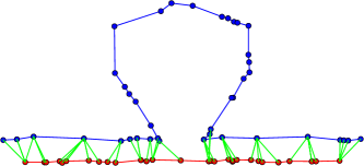
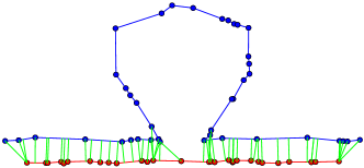
(a)	(b)

Figure 6: Discrete (a) vs semi-continuous (b).

A commonly used model for trajectories is to connect two consecutive sampled points by a line segment — resulting in a polygonal curve. Let $\overline{P}$ and $\overline{Q}$ denote these curves for $P$ and $Q$ respectively. Ideally, we would like to define a monotone assignment as a pair of functions $\alpha:P\rightarrow\overline{Q}\cup\{{\scriptsize\bot}\}$ and $\beta:Q\rightarrow\overline{P}\cup\{{\scriptsize\bot}\}$ and the goal will be to compute a monotone assignment with the maximum score, as defined in (2). This is however, very hard to compute because of the algebraic complexity of the assignment; the description of the points on $\overline{P}$ and $\overline{Q}$ to which $Q$ and $P$ are mapped can be quite large. Because of lack of space, we omit a lower-bound construction from this paper.

We circumvent this problem by sampling points on each edge of $\overline{P}$ and $\overline{Q}$ — for each point $p_{i}\in P$ and every edge $\overline{q_{j}q_{j+1}}$ of $Q$, we sample the closest point of $p_{i}$, $\xi_{i,j}=\arg$ $\min_{x\in\overline{q_{j}q_{j+1}}}\|p_{i}-x\|$ on $\overline{q_{j}q_{j+1}}$. We do the same for every point $q_{k}\in Q$ and every edge $\overline{p_{i}p_{i+1}}$ of $\overline{P}$. Let $P^{*}$ and $Q^{*}$ be the resulting sequence of points. We can then run the previous algorithm on $P^{*}$ and $Q^{*}$. Since $|P^{*}|,|Q^{*}|\leq mn$, the total running time is $O(m^{2}n^{2})$. Besides the high running time, the sampling step is somewhat ad-hoc.

To improve efficiency and avoid this large sampling step, we propose a method of “cheating” to assign points in one trajectory to points in between endpoints in the other trajectory if no endpoint is a good match. At each step of the dynamic programming algorithm, we examine prefixes $P_{i}$ and $Q_{j}$. At this step, we may choose to assign $\alpha(p_{i})=q_{j}$ or $\beta(q_{j})=p_{i}$ depending on their contribution to the overall score which is based on the distance $\|p_{i}-q_{j}\|$. We modify this slightly by assigning $\alpha(p_{i})=\hat{q}_{j-1,j}$ where $\hat{q}_{j-1,j}$ is the closest point on the segment preceding $q_{j}$. Similarly, we assign $\beta(q_{j})=\hat{p}_{i-1,i}$.

Although the assignment is now no longer restricted to be monotone, in practice, we expect that in the similar portions of the trajectories, such an assignment would be monotone and further, it would capture the correspondences better than the discrete setting. Moreover, the running time is now $O(mn)$ which matches the efficiency of the discrete algorithms. Fig. 6 shows a comparison of the two settings for a toy example. This example is very similar to that of Fig. 2 but with different sample points. Note that the semi-continuous model obtains a much more regular set of correspondences of the positions along the trajectories than the discrete setting.

6 Parameter Selection

Parameter selection is an important issue when choosing the scoring function. During the course of the algorithm, when examining a pair of points $p_{i}\in P$ and $q_{j}\in Q$, the difference in values $1/(c+\|p_{i}-q_{j}\|^{2}$ versus $\Delta$ dictate the choice of whether to assign $\alpha(p_{i})=q_{j}$ or $\beta(q_{j})=p_{i}$ versus assigning one or both as gap points.

We work with the hypothesis that all “matched” points have roughly the same distance. Let the threshold on the distance beyond which points are dissimilar be $r$. We suggest the following choices of the parameters:

$$c=\frac{r}{2},\quad\Delta=\frac{1}{c+r^{2}},\quad a=-l\Delta,$$

where $l$ indicates a minimum gap length. If $l=0$, the algorithm simply chooses points which are farther apart than $r$ to be gap points. Otherwise, it only chooses to start gaps when at least $l$ points are farther than $r$ apart since, if not, $a+\Delta\cdot|g|$ will be negative.

The choice of $r$ is clear if we have semantic information about the trajectories such as what type of entities generated them. For example, if we have GPS trajectories from road networks and wish to classify similar portions as those following the same road, then the width of the road and the sampling rate or GPS accuracy would determine the choice of $r$.

On the other hand, in many situations, the choice of $r$ is not clear. For example, if we are given road trajectories but the roads may consist of both highways as well as side streets or alleyways, the widths may vary widely. In such cases, we wish to infer the value of $r$ from the dataset. Unfortunately, this is a hard inference problem. One could use a Bayesian method for this problem, but this is beyond the scope of this paper.

Instead, we use a simple iterative algorithm which proceeds according to the following steps:

• Start with a rough guess of the upper bound $\hat{r}$ and compute an assignment with $r=\hat{r}$.

• Discard a percentage of the larger distances in this assignment and compute the $\mathsf{rms}$ of the remaining distances.

• Choose a new threshold which is a small factor of the $\mathsf{rms}$, say $r=c_{1}\cdot\mathsf{rms}$.

• Repeat steps (2) and (3) until the assignments converge.

When we identify all similar portions and dissimilar portions, we do not expect the $\mathsf{rms}$ to change significantly when we discard some of the larger distances. Hence, the assignments should converge and the algorithm should terminate.

We may set different criteria for termination, particularly if we have additional information. For example, if we have a lower bound on the threshold, we can terminate when we reach this value, since the algorithm need not necessarily terminate at this point. If we know the characteristics of the noise on the measurements, for example, if it is Gaussian, we can fit a Gaussian to the remaining distances and converge when it is a good enough fit.

7 Experiments

We have conducted an experimental study on real datasets to evaluate the effectiveness of our model and to compare with previous approaches. We used the DTW and sequence-alignment based approaches to provide a basis for comparison of our approach. We refer to these algorithms as DTW and Seq-Align and to our algorithm from Sec. 3 as Assignment throughout this section.

Since DTW tries to find correspondences for every point on a trajectory and consequently, does not aim to distinguish between similar and deviating portions, we applied a simple heuristic to make the comparison with Assignment and Seq-Align fairer: after computing the DTW correspondences, we pruned all correspondences where the distance between the two constituent points was greater than a threshold. Recall that the parameter selection for our scoring function (cf. Sec. 6) uses a similar distance threshold $r$. We call this modified DTW heuristic DTW-Pruned.

We present two types of results in this section: (i) an analysis of the nuances of Assignment, DTW and Seq-Align by examining individual pairs of trajectories and their resulting correspondences, and (ii) characteristics of the data based on the correspondences computed over all pairs of trajectories in the datasets. The goal of our experiments was not only to present a qualitative study but also to observe the characteristics of the data and how they impact the model parameters.

7.1 Description of Datasets.

We have used three real datasets in our experiments: (i) the Geolife project by Microsoft Research Asia [29, 30, 28] consisting of 17,621 trajectories of 182 users in China, (ii) 145 trajectories of school buses in Athens, Greece [12], and (iii) 38 trajectories from road cycling exercises captured by a fitness GPS device at a constant one second sample rate. Many of the trajectories in the GeoLife dataset are labeled with the mode of transportation used from the set {biking, walking, running, bus, car, taxi, train, subway, airplane}. We extracted the trajectories with labels in {biking, walking, running} and extracted a sample of trajectories for our experiments. Our subset consists of a total of 883 trajectories. Fig. 7(a) shows the portion of this dataset where trajectories have the highest concentration which is, not surprisingly, in Beijing. Fig. 7(b) and 7(c) shows the other two datasets.

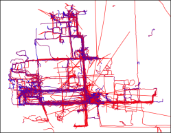
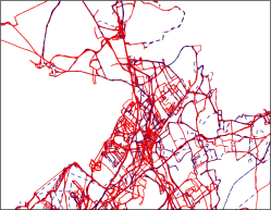
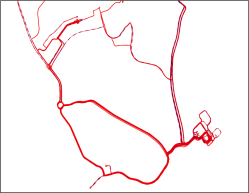
(a)	(b)	(c)

Figure 7: Datasets: (a) GeoLife datasets of trajectories with transportation modes in {biking, walking, running} respectively. (b) Buses dataset, (c) trajectories from road cycling exercises recorded with a fitness GPS device. Sample points are blue while the edges between two points are red.

Although all three datasets are GPS trajectories, they differ significantly from each other due to the different modes of transportation and sensor equipment as well as due to road network characteristicsIn the buses dataset, the sampling rate is fairly infrequent and the data also contains significant measurement noise. On the other hand, although the sampling rate is more frequent for the biking, walking and running trajectories in the GeoLife dataset, here too, it contains significant measurement noise. In addition, there seem to be a large number of partially observed trajectories (long stretches with no samples). The dataset of cycling exercise routes collected is highly accurate and extremely densely sampled making it a good representation of ideal conditions.

7.2 Results on Pairs of Trajectories

To show the effectiveness of our algorithms, we present results on a single pair of trajectories from each of the datasets. We chose the pairs in such a manner that they exhibit significant similar portions as well as dissimilar portions and have sufficiently dissimilar sampling rates in the case of the pairs from the Bus and GeoLife datasets (the cycling exercise trajectories all have a uniform sampling rate). Consequently, the results exhibited on these pairs are representative of the results on other trajectories as well. In all cases, we perturbed one of the trajectories slightly in the figures to present the results more clearly.

Global Assignment.   In each case, we compare the results of Assignment to the results of DTW, DTW-Pruned as well as Seq-Align. We chose a distance threshold $r=100$ m for our parameter selection process for Assignment (see Sec. 6) as well as for DTW-Pruned. The minimum gap length was set at $4$ for both Seq-Align and Assignment. Figures 10, 10 and 10 show the results of computing assignments on the pair of trajectories chosen from each dataset. In the former two, we have also shown in an inset in some cases: a zoomed in portion of the trajectories where the issues with the different approaches are clearer.

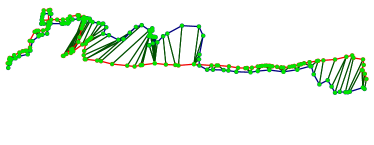
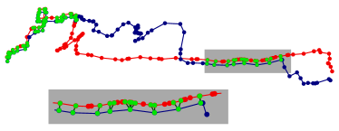
(a) DTW	(b) DTW-Pruned
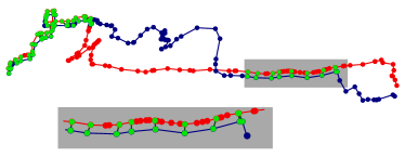
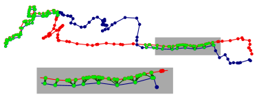
(c) Seq-Align	(d) Assignment

Figure 8: Results on a trajectory pair from the buses dataset.

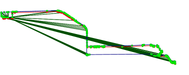
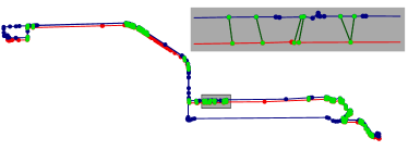
(a) DTW	(b) DTW-Pruned
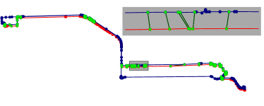
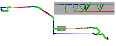
(c) Seq-Align	(d) Assignment

Figure 9: Results on a trajectory pair from the GeoLife dataset.

(a) DTW	(b) DTW-Pruned
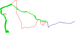
(c) Seq-Align	(d) Assignment

Figure 10: Results on a trajectory pair from the cycling dataset.

The correspondences computed by DTW are clearly not meaningful in differentiating deviating and similar portions (see Figures 10(a), 10(a) and 10(a)). On the other hand, for the buses and GeoLife data, DTW-Pruned clearly does much better in identifying deviations (see Figures 10(b) and 10(b)) but generates a number of smaller gaps due to some correspondences which may be desired having larger distance than the threshold possibly due to measurement noise. Seq-Align which does impose a minimum gap length to get around this issue also has a similar behavior. Here, however, this is caused by the restriction to one-to-one correspondences. Finally, Assignment captures the advantages of the other approaches by generating correspondences for almost all points on the similar portions (see Figure 10(d) and 10(d)). In this case, the imposition of a minimum gap penalty generates correspondences which may be desired in spite of having distance larger than the threshold due to the surrounding correspondences. Due to the allowance of multiple incoming edges for a point in Assignment, the sampling rate issues are also handled well. In the exercise cycling dataset (see Fig. 10), all approaches perform well due to the uniform sampling rate, velocity and accuracy of sampling.

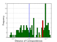
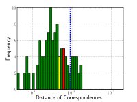
(a) Buses dataset, DTW	(b) Buses dataset, Assignment

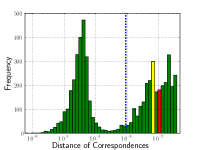
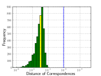
(c) Cycling dataset, DTW	(d) Cycling dataset, Assignment

Figure 11: These histograms summarize the distance between corresponding pairs in the results from Figures 10 and 10. (a) and (b) correspond to Figures 10(a) and 10(d) respectively while (c) and (d) correspond to Figures 10(a) and 10(d) respectively. The bins containing the mean and $\mathsf{rms}$ values are highlighted in yellow and red respectively with no red bin indicating that the $\mathsf{rms}$ and mean lie in the same bin. The vertical blue line denotes the threshold distance.

We also present histograms of the distances of all corresponding pairs for DTW and Assignment for the buses and cycling datasets in Fig. 11. The $x$-axis is set at a log-scale to better visualize the histograms. The bins containing the mean and $\mathsf{rms}$ values are highlighted in yellow and red respectively with no red bin indicating that the $\mathsf{rms}$ and mean lie in the same bin. Comparing Figures 11(a) and 11(b), we notice that the assignment retains some edges whose distance is larger than the threshold $r$ (shown as a blue dashed line). This is due to the minimum gap length constraint which is necessary due to noise in the data. As mentioned above, including correspondences nearby affect the chance of including a correspondence in the result which is more meaningful than simply pruning based on distance as in DTW-Pruned.

Local and Semi-Continuous Assignment.   We present qualitative results for local and semi-continuous assignments. Fig. 13 compares the discrete and semi-continuous assignments for the trajectories chosen from the bus dataset. For the semi-continuous case, we have used the method of choosing the closest point during the course of our algorithm described in Section 5 and not the up-sampling approach. Note the regularity of the segments indicating the correspondences (shown in green) as compared to the discrete setting. This is also a good indication that the variance of assigned distances is much smaller and reflects the characteristics of the routes taken by the trajectories.

Fig. 13 shows the best of the individual local assignments computed for the pair of trajectories chosen from the bus dataset under both the discrete and semi-continuous setting. We chose the parameter $\tau$ used to decide a lower bound on the scores of the local assignment (see Sec. 4) to be $1.5\Delta$ and $2\Delta$ respectively for the discrete and semi-continuous cases. On the other hand, the local assignment computed in the discrete setting captures a shorter portion where the sampling is more uniform.

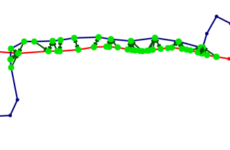
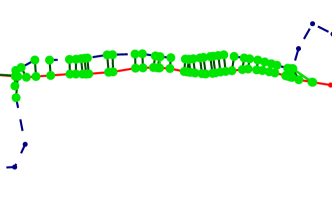
(a) Discrete	(b) Semi-continuous

Figure 12: Comparison of discrete and semi-continuous assignments.

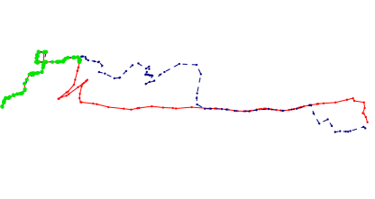
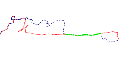
(a) Discrete	(b) Semi-continuous

Figure 13: Local assignments.

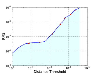
Figure 14: Illustration of the root-mean-square of distances between the pairs in the optimal assignment as a function of the distance threshold used to define the parameters of $\sigma$ (cf. Section 6). The red dots on the curve corresponds to the $\mathsf{rms}$ values produced during the iterative parameter selection algorithm.

(a)	(b)	(c)
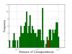
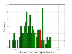
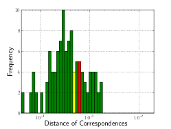
(d)	(e)	(f)
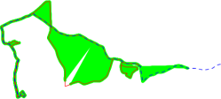
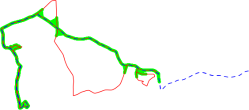
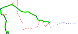
(g)	(h)	(i)
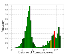
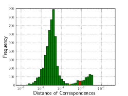
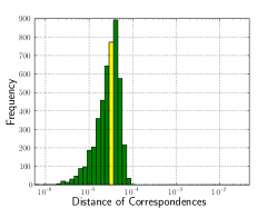
(j)	(k)	(l)

Figure 15: The assignments and corresponding distance histograms computed at various stages of the iterative algorithm. (a), (b), (c), (d), (e) and (f) correspond to the buses dataset pair while (g), (h), (i), (j), (k) and (l) correspond to the cycling dataset pair. (a), (d), (g) and (j) are at the first iteration, (b), (e), (h) and (k) are at an intermediate stage and (c), (f), (i) and (l) are at the point of convergence.

Effect of Parameters.   Recall that the parameters in the scoring function are all set based on a threshold distance for gaps (see Sec. 6). Fig. 14 shows how the $\mathsf{rms}$ of the optimal assignment varies as a function of the distance threshold $r$ used to define the parameters of $\sigma$. For each distance $r$ on the $x$-axis we defined the parameters $a,\Delta,c$ and computed the $\mathsf{rms}$ of the optimal assignment based on those parameters. The axes in Fig. 14 are set at a log-scale due to the much larger variation in distances and extremely low distance threshold in the converged assignment. When we choose the “correct” $r$ for the algorithm, we expect variation in distances of assignment edges to be only due to noise. Hence, the $\mathsf{rms}$ of the assignment edges will be comparable to the chosen $r$ (if the actually deviating portions are at sufficiently large distances relative to the noise). This is reflected in the flat portion of the graph in Fig 14. The red points in Fig. 14 are the chosen thresholds of the iterative procedure and as can be seen, it converges (leftmost red point) when the chosen threshold is comparable to the $\mathsf{rms}$.

Finally, Fig. 15 shows the assignment and histograms for the pair from the buses and cycling datasets at the beginning, end and an intermediate step of the iterative approach. As we can see, larger distances are slowly pruned away until we reach the optimal assignment. In the bus dataset, however, there is still significant variance in the data at the time of convergence showing the low sampling rate and noise inherent in the data.

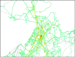
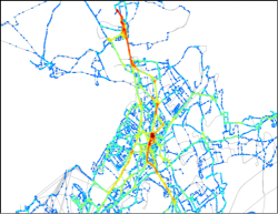
(a) DTW	(b) DTW-Pruned	(c) Assignment
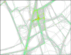
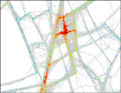
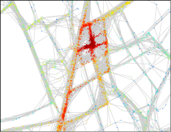
(d) DTW	(e) DTW-Pruned	(f) Assignment

Figure 16: Heat maps of the importance of sample points for the buses dataset. (d), (e) and (f) show a zoomed in portion of (a), (b) and (c) respectively.

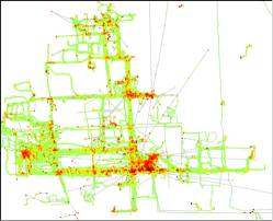
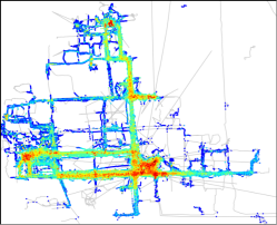
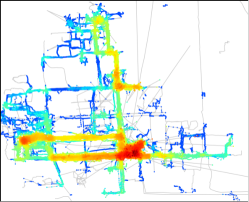
(a) DTW	(b) DTW-Pruned	(c) Assignment

Figure 17: Heat maps of the importance of sample points for the GeoLife dataset.

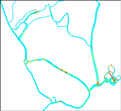
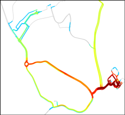
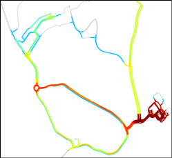
(a) DTW	(b) DTW-Pruned	(c) Assignment

Figure 18: Heat maps of the importance of sample points for the cycling dataset.

7.3 Results on Complete Datasets

To further demonstrate the effectiveness of our algorithms, we present here results showing the behavior on the datasets as a whole. Based on pairwise correspondences computed by the DTW, DTW-Pruned and Assignment algorithms, we analyze the importance of a sample point on a trajectory based on its correspondences with all other trajectories. Specifically, we wish to measure the importance of a portion of a trajectory with respect to the dataset using the importance of individual points on it. In all cases, we compute pairwise correspondences for all pairs of trajectories in the dataset. Based on these, we define the importance of a sample point $p$ on some trajectory $P$ in three different ways for the three algorithms such that the comparison is as fair as possible: (i) for Assignment, we define it as the number of outgoing edges for a sample point, i.e., the number of trajectories $Q$ such that for some $q\in Q$, $\alpha(p)=q$ in the assignment., (ii) for DTW-Pruned, we define it in a similar manner, the number of trajectories $Q$ such that $(p,q)$ for some $q\in Q$ is part of the set of correspondences between $P$ and $Q$, (iii) for DTW, it is not possible to define similar to DTW-Pruned since then, the importance of all points is the same; hence, we define it as the number of correspondence pairs that $p$ is part of over all pairwise assignments. For Assignment, the outdegree of a point is an intuitive way to define the importance since it provides a natural way of defining the number of trajectories which share a common portion with $P$ at $p$. We chose the definition of importance of DTW-Pruned to reflect the same intuition.

Again, we chose 100 m as the distance threshold for DTW-Pruned and Assignment and 4 as the minimum gap length for Assignment. Figures 18, 18 and 18 show the heat maps of the importance of the points belonging to all trajectories in the buses, GeoLife and cycling datasets respectively. As is clear, the DTW approach does not provide any meaningful results, so we present it for completeness. Comparing DTW-Pruned and Assignment, the results are quite similar. Both of these seem to do a good job of identifying commonly traveled routes and landmark points in the dataset. Assignment seems to do a slightly better job of identifying more central points along the routes or points on a so-called “mean” trajectory although this is apparent only upon close examination. Further analyzing the behavior of trajectories based on the complete dataset is outside the scope of this paper and we present these results here as a flavor of what our framework can provide for this purpose.

7.4 Summary

We have shown that our framework captures the advantages of both DTW and sequence alignment based approaches for identifying trajectory similarity, and that it is able to exceed their accuracy. Experiments show that the approach is highly accurate in identifying similar portions of trajectories from real datasets. Further, even without an accurate prior knowledge of distances between points based on which to compute similarity, our iterative procedure is able to converge at the point where similar portions are identified and distinguished accurately from dissimilar portions. We also show the effectiveness of the semi-continuous setting and that the shift of the score for computing local assignment is highly dependent on the variance of distances between similar points.

Finally, our results on importance of sample points based on pairwise correspondences computed over the entire dataset shows that our framework does as well or better than other approaches while provided a principled way to compute correspondences and measure similarity between two trajectories. We feel that, for the purposes of analyzing complete datasets for highly conserved portions of trajectories and performing clustering of trajectories on this basis, our framework of assignments provides a solid foundation to work with. This direction of research certainly seems like a rich one to undertake.

References

- [1] Pankaj K. Agarwal, Rinat Ben Avraham, Haim Kaplan, and Micha Sharir. Computing the Discrete Fréchet Distance in Subquadratic Time. In Proc. 24th ACM-SIAM SODA, pages 156–167, 2013.
- [2] Helmut Alt and Michael Godau. Computing the Fréchet Distance between Two Polygonal Curves. Int. J. Comput. Geometry Appl., 5:75–91, 1995.
- [3] Helmut Alt and Leonidas J. Guibas. Discrete Geometric Shapes: Matching, Interpolation, and Approximation. In Handbook of Computational Geometry, pages 121–153. Elsevier, 2000.
- [4] Kevin Buchin, Maike Buchin, Marc van Kreveld, and Jun Luo. Finding Long and Similar Parts of Trajectories. Comput. Geom., 44(9):465–476, 2011.
- [5] Kevin Buchin, Maike Buchin, and Yusu Wang. Exact Algorithm for Partial Curve Matching via the Fréchet Distance. In Proc. 20th ACM-SIAM SODA, pages 645–654, 2009.
- [6] Lei Chen and Raymond Ng. On the marriage of lp-norms and edit distance. In Proc. VLDB, pages 792–803, 2004.
- [7] Lei Chen, M. Tamer Özsu, and Vincent Oria. Robust and Fast Similarity Search for Moving Object Trajectories. In Proc. ACM SIGMOD, pages 491–502, 2005.
- [8] Defense Systems. Soldiers gain combat edge with smart helmets . http://defensesystems.com/articles/2009/05/06/defense-it-3-helmet-networks.aspx, 2009.
- [9] Hui Ding, Goce Trajcevski, Peter Scheuermann, Xiaoyue Wang, and Eamonn Keogh. Querying and Mining of Time Series Data: Experimental Comparison of Representations and Distance Measures. In Proc. VLDB, pages 1542–1552, 2008.
- [10] R Durbin, S R Eddy, A Krogh, and G Mitchison. Biological Sequence Analysis: Probabilistic Models of Proteins and Nucleic Acids. Cambridge University Press, 1998.
- [11] Sigal Elnekave, Mark Last, and Oded Maimon. Incremental Clustering of Mobile Objects. In IEEE ICDE Workshops, pages 585–592, 2007.
- [12] Elias Frentzos, Kostas Gratsias, Nikos Pelekis, and Yannis Theodoridis. Nearest Neighbor Search on Moving Object Trajectories. In Claudia Bauzer Medeiros, MaxJ. Egenhofer, and Elisa Bertino, editors, Advances in Spatial and Temporal Databases, volume 3633 of Lecture Notes in Computer Science, pages 328–345. Springer Berlin Heidelberg, 2005.
- [13] Joachim Gudmundsson, Marc Kreveld, and Bettina Speckmann. Efficient Detection of Patterns in 2D Trajectories of Moving Points. GeoInformatica, 11(2):195–215, 2007.
- [14] Shoji Hirano and Shusaku Tsumoto. A Clustering Method for Spatio-temporal Data and Its Application to Soccer Game Records. In Dominik Ślęzak, Guoyin Wang, Marcin Szczuka, Ivo Düntsch, and Yiyu Yao, editors, Rough Sets, Fuzzy Sets, Data Mining, and Granular Computing, volume 3641 of Lecture Notes in Computer Science, pages 612–621. Springer Berlin Heidelberg, 2005.
- [15] D. S. Hirschberg. A Linear Space Algorithm for Computing Maximal Common Subsequences. Commun. ACM, 18(6):341–343, 1975.
- [16] Patrick Laube. Finding REMO : Detecting Relative Motion Patterns in Geospatial Lifelines. Developments in Spatial Data Handling, pages 201–215, 2005.
- [17] Jae-Gil Lee, Jiawei Han, and Kyu-Young Whang. Trajectory Clustering: A Partition-and-Group Framework. In Proc. ACM SIGMOD, pages 593–604, 2007.
- [18] Tim Meyer, Marco D’Abramo, Adam Hospital, Manuel Rueda, Carles Ferrer-Costa, Alberto Pérez, Oliver Carrillo, Jordi Camps, Carles Fenollosa, Dmitry Repchevsky, Josep Lluis Gelpí, and Modesto Orozco. MoDEL (Molecular Dynamics Extended Library): A Database of Atomistic Molecular Dynamics Trajectories. Structure, 18(11):1399–1409, 2010.
- [19] Saul B. Needleman and Christian D. Wunsch. A General Method Applicable to the Search for Similarities in the Amino Acid Sequence of Two Proteins. J. Mol. Biol., 48(3):443–453, 1970.
- [20] Claudio Piciarelli, Christian Micheloni, and G.L. Foresti. Trajectory-Based Anomalous Event Detection. IEEE Trans. Circuits Syst. Video Technol., 18(11):1544–1554, 2008.
- [21] L.R. Rabiner and B.H. Juang. Fundamentals of Speech Recognition. Prentice Hall Signal Processing Series. PTR Prentice Hall, 1993.
- [22] Yossi Rubner, Carlo Tomasi, and Leonidas J. Guibas. The Earth Mover’s Distance as a Metric for Image Retrieval. Int. J. Comput. Vision, 40(2):99–121, 2000.
- [23] T.F. Smith and M.S. Waterman. Identification of Common Molecular Subsequences. J. Mol. Biol., 147(1):195–197, 1981.
- [24] The Wall Street Journal. Apple, Google collect user data . http://online.wsj.com/article/SB10001424052748703983704576277101723453610.html, 2011.
- [25] Michail Vlachos, Dimitrios Gunopoulos, and George Kollios. Discovering Similar Multidimensional Trajectories. In Proc. 18th IEEE ICDE, pages 673–684, 2002.
- [26] Yin Wang, Yanmin Zhu, Zhaocheng He, Yang Yue, and Qingquan Li. Challenges and opportunities in exploiting large-scale gps probe data. Technical Report HPL-2011-109, HP Laboratories, 2011.
- [27] T. Wolle and J. Gudmundsson. Towards Automated Football Analysis: Algorithms and Data Structures. In Proc. 10th Australasian Conference on Mathematics and Computers in Sport (ACMCS), 2010.
- [28] Yu Zheng, Quannan Li, Yukun Chen, Xing Xie, and Wei-Ying Ma. Understanding Mobility Based on GPS Data. In Proc. 10th ACM UbiComp, pages 312–321, 2008.
- [29] Yu Zheng, Xing Xie, and Wei-Ying Ma. GeoLife: A Collaborative Social Networking Service among User, Location and Trajectory. IEEE Data Eng. Bull., 33(2):32–39, 2010.
- [30] Yu Zheng, Lizhu Zhang, Xing Xie, and Wei-Ying Ma. Mining Interesting Locations and Travel Sequences from GPS Trajectories. In Proc. 18th ACM WWW, pages 791–800, 2009.