Controlled ripple texturing of suspended graphene membrane due to coupling with ultracold atoms

Abstract

We explore the possibility to create hybrid quantum systems that combine ultracold atoms with graphene membranes. We investigate a setup in which a cold atom cloud is placed close to a free–standing sheet of graphene at distances of a few hundred nanometers. The atoms then couple strongly to the graphene membrane via Casimir–Polder forces. Temporal changes in the atomic state of the atomic cloud changes the Casimir–Polder interaction, thereby leading to the creation of a backaction force in the graphene sheet. This setup provides a controllable way to engineer ripples in a graphene sheet with cold atoms.

With the advances in trapping and coherently manipulating clouds of ultracold atoms near microstructured solid-state surfaces Reichel and Vuletić (2011), the possibility of constructing hybrid atom/solid-state quantum systems have attracted considerable attention (see, e.g., Refs. Hammerer et al. (2009); Wallquist et al. (2009); Hunger et al. (2011); Treutlein et al. ). Such a hybrid system would consist of ultracold atoms that can be manipulated by laser light, and a solid-state system that could for instance be controlled by electrical currents. The influence of the solid-state substrate on the atomic dynamics is well established; dispersion potentials Scheel and Buhmann (2008) and their consequences such as quantum reflection Pasquini et al. (2004) and line shifts Kübler et al. (2010) are sufficiently well understood. However, a backaction of the atom cloud on the solid-state system is rather challenging. If atoms are regarded as mechanical oscillators Hunger et al. (2011), the impedance mismatch due to the large mass difference between a single atom and a mechanical oscillator limits the atom–surface coupling. The routes that have been taken so far to alleviate this discrepancy are either to select a subsystem within the solid-state device Hunger et al. (2011), to decrease the effective size of the macroscopic system Fermani et al. (2007); Schneeweiss et al. (2012), or to enhance the coupling of ions to a membrane via resonant modes of an optical cavity Hammerer et al. (2009); Wallquist et al. (2009). It has been proposed that laser light could be used to couple also the motion of ultracold trapped atoms to the vibrational modes of a mechanical oscillator. In recent experiments, using magnetic Wang et al. (2006) or surface–force coupling Hunger et al. (2010), atoms are used to study vibrations of micromechanical oscillators. In Ref. Camerer et al. (2011), the backaction of the atoms onto the oscillator vibrations as well as the effect of the membrane vibrations onto the atoms were observed.

Our goal is to find a coupling mechanism between ultracold atoms and a solid-state system that is strong enough to provide a mutual interaction between them. In this article we show that the Casimir–Polder force Scheel and Buhmann (2008), a dispersion interaction that is due to quantum fluctuations of the electromagnetic field, can provide precisely that. The Casimir-Polder force on an atom in thermal equilibrium with its environment is typically attractive; however, in out-of-equilibrium situations such as for atoms prepared in energy eigenstates the sign of that force can be reversed Buhmann and Scheel (2008) and can reach extremely large values for highly excited (Rydberg) atoms Crosse et al. (2010). Any cycling transition between the ground state and an excited state thus translates into an oscillating dispersion force. The coupling could be increased by minimizing the impedance mismatch using oscillators with low mass such as carbon nanotubes or graphene membranes. Freely suspended graphene crystals can exist without a substrate, suspended graphene flakes or scaffolds have been observed for single layers and bilayers Meyer et al. (2007). Suspended graphene membranes can be created with diameters that are comparable to the diameter of a Bose–Einstein condensate. Free-standing graphene membranes have a key advantage over bulk systems studied in previous works as the membrane can be cleaned from adsorbates by passing a current through it Judd et al. (2011).

In the resulting hybrid quantum system, driving the atomic cloud to excited states could be used to engineer ripples on a graphene membrane. Ripples are an intrinsic feature of graphene sheets which influence their electronic properties; perturbations to nearest neighbour hopping might cause the same effects as inducing an effective magnetic fields and changing local potentials Morozov et al. (2006); Pereira and Castro Neto (2009); Pereira et al. (2010). The ability to control ripple structures could allow a device design based on local strain and selective bandgap engineering Neto and Novoselov (2011). The possibility of constructing an all-graphene circuit, one of the big goals in graphene science, could be achieved by applying the patterning of different devices and leads by means of appropriate cuts in the sheet. In Ref. Pereira and Castro Neto (2009) it has been proposed to deposit graphene onto substrates with regions that can be controllably strained on demand, or by exploring substrates with thermal expansion heterogeneity; the generation of strain in the graphene lattice is then capable of changing the in-plane hopping amplitude in an anisotropic way. Controlled ripple texturing using both spontaneously and thermally generated strains was first reported in Ref. Bao et al. (2009), where the possibility was shown to control ripple orientation, wavelength and amplitude by controlling boundary conditions and making use of graphene’s negative thermal expansion coefficient.

In the following, we evaluate the Casimir-Polder force between a single graphene sheet and a rubidium atom in various energy eigenstates and determine the minimal number of atoms needed to excite a ripple. For the calculation of the interaction potential we assume the sheet to be infinitely extended, thereby neglecting possible effects that may arise from the finite extent of the flake. For planar structures, the Casimir-Polder potential of an atom in an energy eigenstate $\displaystyle|n\rangle$ at a distance $\displaystyle z_{A}$ away from the macroscopic body with permittivity $\displaystyle\varepsilon(\omega)$ can be written as Scheel and Buhmann (2008)

$$\displaystyle U_{\mathrm{CP}}\left(z_{A}\right)=\frac{\hbar\mu_{0}}{8\pi^{2}}\int_{0}^{\infty}d\xi\,\xi^{2}\alpha_{n}(i\xi)\int\limits_{0}^{\infty}dk_{\parallel}\frac{e^{-2k_{\parallel}\gamma_{0z}z_{A}}}{\gamma_{0z}}$$

$$\displaystyle\times\left[\mathrm{R}_{\mathrm{TE}}+\mathrm{R}_{\mathrm{TM}}\left(1-\frac{2k_{\parallel}^{2}\gamma_{0z}^{2}c^{2}}{\xi^{2}}\right)\right]$$

$$\displaystyle+\frac{\mu_{0}}{4\pi}\sum_{k\neq n}\omega_{nk}^{2}\mathbf{d}_{nk}\otimes\mathbf{d}_{kn}\int_{0}^{\infty}d\kappa_{0z}e^{-2\kappa_{0z}}$$

$$\displaystyle\times\mathrm{Re}\left[\mathrm{R}_{\mathrm{TE}}+\mathrm{R}_{\mathrm{TM}}\left(1+\frac{2\kappa_{0z}^{2}c^{2}}{\omega^{2}}\right)\right].$$ (1)

where $\displaystyle\gamma_{iz}=\sqrt{1+\varepsilon(i\xi)\xi^{2}/(c^{2}k_{\|}^{2})}$, $\displaystyle\kappa_{0z}=\sqrt{k_{\|}^{2}+\omega^{2}/c^{2}}$ and $\displaystyle\alpha_{n}(\omega)$ is the atomic polarizability defined by

$$\mathbf{\alpha}_{n}(\omega)=\lim_{\varepsilon\rightarrow 0}\frac{2}{\hbar}\sum_{k\neq n}\frac{\omega_{kn}\mathbf{d}_{nk}\otimes\mathbf{d}_{kn}}{\omega_{kn}^{2}-\omega^{2}-i\omega\varepsilon}\,.$$ (2)

The first term in Eq. (1) describes the nonresonant part of the Casimir-Polder potential, recognisable by the integration along the imaginary frequency axis, $\displaystyle\omega=i\xi$, whereas the second term is related to resonant photon exchange between the atom and the graphene sheet. Equation (1) is strictly valid only at zero temperature. However, we can assume that a potential experiment with ultracold atoms could be performed at sufficiently low temperatures for thermal excitations to only play a subordinant role; in addition, the distance of those atoms from the graphene sheet will be much smaller than the thermal wavelength $\displaystyle\lambda_{T}=hc/(k_{B}T)$. In situations in which either assumption fails to hold, a replacement of the frequency integral by a Matsubara sum,

$$\frac{\hbar}{\pi}\int\limits_{0}^{\infty}d\xi\,f(i\xi)\mapsto 2k_{B}T\sum\limits_{n=0}^{\infty}\left(1-\frac{1}{2}\delta_{0n}\right)f(i\xi_{n})\,,$$ (3)

with Matsubara frequencies $\displaystyle\xi_{n}=n2\pi k_{B}T/\hbar$ Buhmann and Scheel (2008), has to be employed. The material properties of graphene enter via their reflection coefficients $\displaystyle\mathrm{R}_{\mathrm{TE}}$ and $\displaystyle\mathrm{R}_{\mathrm{TM}}$. Due to graphene’s unique electronic structure, a full calculation of its electromagnetic reflection coefficients is in fact possible from first principles. Following Ref. Fialkovsky et al. (2011), in order to derive the reflection coefficient of a graphene sheet, the dynamics of quasiparticles are described within the (2+1)–dimensional Dirac model. The quasiparticles in graphene obey the linear dispersion law $\displaystyle\omega=v_{F}k$, where $\displaystyle v_{F}\approx c/300$ is the Fermi velocity valid for energies below 2 eV Peres (2010). More elaborate models for the conductivity are not needed here because at frequencies above the dominant atomic transitions the polarizability $\displaystyle\alpha_{n}(i\xi)$ does no longer contribute to the integral in Eq. (1).

Thermal corrections become important only for $\displaystyle k_{B}T\gtrsim\Delta$, where $\displaystyle\Delta$nis the gap parameter of quasiparticle excitations Chaichian et al. (2012). At finite temperature, the potential is well approximated by inserting the temperature-dependent reflection coefficients in the lowest term in the Matsubara sum ($\displaystyle j=0$) while keeping the zero-temperature coefficients for all higher Matsubara terms. However, it has been shown in Ref. Drosdoff and Woods (2010), that at room temperature the static value of the polarizability increases only by 10 percent. The TM reflection coefficient increases by one percent due to finite temperature and the TE coefficient vanishes altogether at zero frequency. For this reason and with the similar approach in Ref. Sernelius (2012) in mind, we have used the zero-temperature limit of the polarizability as a very good approximation.

The interaction of the quasiparticles with external electromagnetic fields can be described within this Dirac model. From the boundary conditions of the electric and magnetic fields one finds the reflection and transmission coefficients given the specific values of mass gap $\displaystyle m$ and chemical potential $\displaystyle\mu$. For simplicity we will set $\displaystyle m=\mu=0$ (perfect Dirac cone) for which the difference between this approximation for suspended graphene samples ($\displaystyle m,\mu\sim 0.01$eV) is less than $\displaystyle 1\%$ Fialkovsky et al. (2011). One then arrives at the reflection coefficients of a free standing graphene sheet in vacuum as

$$\displaystyle\mathrm{R}_{\mathrm{TM}} \displaystyle= \displaystyle\frac{4\pi\alpha\sqrt{k_{0}^{2}+k_{\parallel}^{2}}}{4\pi\alpha\sqrt{k_{0}^{2}+k_{\parallel}^{2}}+8\sqrt{k_{0}^{2}+\tilde{v}^{2}k_{\parallel}^{2}}}\,,$$ (4)

$$\displaystyle\mathrm{R}_{\mathrm{TE}} \displaystyle= \displaystyle-\frac{4\pi\alpha\sqrt{k_{0}^{2}+\tilde{v}^{2}k_{\parallel}^{2}}}{4\pi\alpha\sqrt{k_{0}^{2}+\tilde{v}^{2}k_{\parallel}^{2}}+8\sqrt{k_{0}^{2}+k_{\parallel}^{2}}}\,,$$ (5)

where we defined $\displaystyle k_{0}^{2}=\xi^{2}/c^{2}$ and $\displaystyle\tilde{v}=v_{F}/c=(300)^{-1}$; $\displaystyle\alpha=1/137$ is the fine structure constant.

For a ground-state rubidium atom the force $\displaystyle\mathbf{F}_{\mathrm{CP}}\left(z_{A}\right)=-\bm{\nabla}_{A}U_{\mathrm{CP}}\left(z_{A}\right)$ at $\displaystyle z_{A}=200$ nm is rather small — $\displaystyle F_{\mathrm{CP}}(5S_{1/2})=-1.05\times 10^{-22}$ N. The atom–surface coupling can be vastly enhanced by promoting atoms to highly excited Rydberg states, i.e. states with very high principal quantum number $\displaystyle n$.

The primary motivation for the study of Rydberg atoms is to take advantage of the unique opportunities afforded by their exaggerated properties which make them extremely sensitive to small-scale perturbations of their environment and to dispersion forces. A second important aspect of atoms in Rydberg states is their regularity Gallagher (1988). For example, the free-space radiative lifetime of high-lying Rydberg states increases as $\displaystyle n^{3}$. The influence of macroscopic bodies modifies those atomic relaxation rates Scheel and Buhmann (2008). Earlier results Crosse et al. (2010) showed a strong enhancement in the transition rates of Rydberg atoms near a surface. Intimately connected (via a Hilbert transform or Kramers–Kronig relation) to the lifetime is the dispersive energy shift that a Rydberg atom experiences in the vicinity of a macroscopic body (Casimir-Polder shift) Crosse et al. (2010) or in close proximity of another atom (van der Waals shift). An important consequence of the latter is the Rydberg blockade effect that prevents multiple Rydberg excitations within a volume of radius $\displaystyle a_{\mathrm{block}}$, the blockade radius Gaëtan et al. (2009).

Table 1: Casimir-Polder force between rubidium atoms in different atomic states and graphene sheet and the number of atoms needed to excite a ripple of $\displaystyle 1$ nm amplitude.

Atomic State	$\displaystyle T=0$K		$\displaystyle T=300$K
	$\displaystyle F_{\mathrm{CP}}(N)$	$\displaystyle N_{\mathrm{atoms}}$	$\displaystyle F_{\mathrm{CP}}(N)$	$\displaystyle N_{\mathrm{atoms}}$
$\displaystyle z_{A}=200$ nm
$\displaystyle\left|26S_{1/2}\right\rangle$	$\displaystyle 2.29\times 10^{-16}$	70	$\displaystyle-1.89\times 10^{-15}$	9
$\displaystyle\left|29S_{1/2}\right\rangle$	$\displaystyle 3.72\times 10^{-16}$	43	$\displaystyle-4.08\times 10^{-15}$	4
$\displaystyle\left|32S_{1/2}\right\rangle$	$\displaystyle 5.72\times 10^{-16}$	28	$\displaystyle-8.15\times 10^{-15}$	2
$\displaystyle\left|34S_{1/2}\right\rangle$	$\displaystyle 7.47\times 10^{-16}$	22	$\displaystyle-1.25\times 10^{-14}$	2
$\displaystyle z_{A}=z_{\mathrm{min}}(n)$
$\displaystyle\left|26S_{1/2}\right\rangle$	$\displaystyle 8.88\times 10^{-15}$	2	$\displaystyle-7.36\times 10^{-14}$	1
$\displaystyle\left|29S_{1/2}\right\rangle$	$\displaystyle 6.04\times 10^{-15}$	3	$\displaystyle-6.65\times 10^{-14}$	1
$\displaystyle\left|32S_{1/2}\right\rangle$	$\displaystyle 4.25\times 10^{-15}$	4	$\displaystyle-6.05\times 10^{-14}$	1
$\displaystyle\left|34S_{1/2}\right\rangle$	$\displaystyle 3.41\times 10^{-15}$	5	$\displaystyle-5.69\times 10^{-14}$	1

In Table 1 we show numerical values of the Casimir-Polder force acting on rubidium atoms. One observes that the force is attractive for ground-state atoms, but repulsive for highly excited atoms. This is due to the increased contributions of the resonant Casimir-Polder force associated with real-photon transitions as opposed to the nonresonant force components due to virtual-photon exchanges. A handy feature of Rydberg atoms is thus the tunability of their interaction strength by choosing a particular Rydberg state Gallagher (1988); Löw et al. (2012). The excitation into Rydberg states with principal quantum numbers ranging from $\displaystyle n=20$ up to the ionization threshold are typically accomplished by a two–photon excitation scheme (for an experimental review see Löw et al. (2012)). Positioning the atom cloud at a fixed distance away from the surface, one can then excite atoms to the desired Rydberg state. The backaction of the atoms, mediated by the Casimir-Polder force, onto the membrane will be a periodic bending force $\displaystyle F_{b}$. Thus, when driving an atom from its ground state to a Rydberg state and back, one cycles between an attractive (when the atom is in the ground state) and a repulsive interaction (when the atom is in the Rydberg state) between atom and graphene sheet. In addition it is well known that a free–floating graphene sheet would always crumple at room temperature, hence the need to support the graphene sheet by a substrate. At very low temperatures, the graphene membrane experiences a combination of the following forces: (a) the substrate–pinning force $\displaystyle F_{pin}$ that prevents the graphene membrane from sliding and (b) the bending force $\displaystyle F_{b}$ due to the Casimir-Polder potential, see Fig. 1.

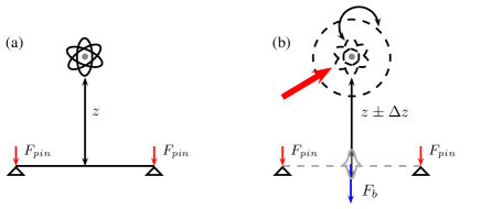
Figure 1: (Color online) Schematic diagram (not to scale) showing an atom next to a suspended graphene membrane. The arrows indicate the two forces $\displaystyle F_{pin}$, $\displaystyle F_{b}$ at interplay in the system.

Measurements on layered graphene sheets of thickness between 2 and 8 nm have provided spring constants that scale as expected with the dimensions of the suspended section, and range from 1 to 5 N/m Franck et al. (2007). Other experiments studied the fundamental resonant frequencies from electromechanical resonators made from graphene sheets Bunch et al. (2007). For mechanical resonators under tension $\displaystyle T$ the fundamental resonance mode $\displaystyle f_{0}$ is given by

$$f_{0}=\left\{\left[A\sqrt{\frac{E}{\rho}}\frac{t}{L^{2}}\right]^{2}+A^{2}0.57\frac{T}{\rho L^{2}wt}\right\}^{1/2}$$ (6)

where $\displaystyle E$ is Young’s modulus, $\displaystyle\rho$ is the mass density; $\displaystyle t,\,w,\,L$ are the thickness, width and length of the suspended graphene sheet and $\displaystyle A$ is a clamping coefficient ($\displaystyle A$ is equal to 1.03 for doubly clamped beams and 0.162 for cantilevers). The effective spring constant of the fundamental resonance mode is given by $\displaystyle\kappa_{\mathrm{eff}}=m_{\mathrm{eff}}\omega^{2}$, where $\displaystyle m_{\mathrm{eff}}=0.735Lwt\rho$ Bunch et al. (2007). In the limit of vanishing tension, the fundamental resonance mode is $\displaystyle f_{0}=A\sqrt{E/\rho}\>t/L^{2}$. However, we have to assume a finite value for the tension, for which we choose $\displaystyle T=0.1$ nN. Tension between graphene and trenches is a random process depending on the production technique and the interaction with the substrate and for that reason very difficult to control Bunch et al. (2007). Using the known values for bulk graphite $\displaystyle\rho=2200$ kg/m³ and $\displaystyle E=1.0$ TPa, for a graphene cantilever with $\displaystyle t=$0.3 nm, $\displaystyle L=$3 $\displaystyle\mu$m and $\displaystyle w=$2 $\displaystyle\mu$m the force needed to create a curvature on graphene with 1 nm amplitude is approximately $\displaystyle 16$ fN. In order to create a force necessary to produce a ripple of a determined amplitude — AFM imaging measures amplitudes in graphene sheets from 0.7 to 30 nm Bao et al. (2009) — one has to excite a particular number $\displaystyle N$ of atoms from the cloud.

Upon inspection of Table 1 one observes that, for a cloud of cold ⁸⁷Rb atoms at a fixed distance of 200 nm from the graphene membrane, one would need to excite one or more atoms in order to create a ripple with 1 nm amplitude. With the blockade radius $\displaystyle a_{\mathrm{block}}$ of several micrometers between neighbouring Rydberg atoms only a limited number of atoms can be resonantly excited to Rydberg states at the same time. If larger numbers of Rydberg excitations are needed, the laser line width has to be chosen large enough to bridge the van der Waals shift between two neighbouring Rydberg atoms. This is easily achieved by pulsed-laser excitation with typical line widths of several $\displaystyle 10-100$ MHz.

The interplay between atom–surface distance and principal quantum number $\displaystyle n$ is of crucial importance in this process. For fixed atom–surface distance, the interaction increases with $\displaystyle n$ so that fewer atoms are needed to induce a desired ripple amplitude. However, due to its increasing size, there is a limit to how close a Rydberg atom can possibly be brought to a surface, or to what Rydberg state an atom at a given distance can be excited. This limiting distance can be estimated simply from the classical atomic radius as $\displaystyle z_{\mathrm{min}}(n)\gtrsim\sqrt{5}n^{2}a_{B}$ where $\displaystyle a_{B}$ is the Bohr radius and the numerical factor $\displaystyle\sqrt{5}$ has been chosen to ensure that its wavefunction does not overlap with the surface. We see that the number of atoms decreases when placed at their minimal distance and, at finite temperature, this number may decrease to only one atom needed to create a 1 nm ripple.

Table 2: Minimal number of atoms required to generate a ripple with 1 nm amplitude. The atoms are assumed to be held at their respective minimal distances at zero temperature.

Atomic State	$\displaystyle z_{\mathrm{min}}(n)$	$\displaystyle N_{\mathrm{min}}(n)$
$\displaystyle\left|23S_{1/2}\right\rangle$	$\displaystyle 62$ nm	1
$\displaystyle\left|30S_{1/2}\right\rangle$	$\displaystyle 106$ nm	3
$\displaystyle\left|36S_{1/2}\right\rangle$	$\displaystyle 153$ nm	6
$\displaystyle\left|43S_{1/2}\right\rangle$	$\displaystyle 218$ nm	12

An estimate of the number of atoms in a given Rydberg $\displaystyle n$ state needed to generate a ripple with amplitude 1 nm can thus be obtained as follows. From Ref. Crosse et al. (2010) we know that the Casimir-Polder force in the non-retarded limit scales as $\displaystyle F_{\mathrm{CP}}\propto n^{4}/z^{4}$. We then equate the necessary number of atoms to generate a force of, say $\displaystyle 16$ fN, by using the scaling law on a particular reference state, say $\displaystyle 32S$ from Table 1 at zero temperature. Together with the constraint on distance, $\displaystyle z_{\mathrm{min}}(n)\gtrsim n^{2}(0.118\,\mbox{nm})$, this yields a lower bound on the number of required atoms as $\displaystyle N_{\mathrm{min}}(n)\gtrsim 3.6\times 10^{-6}n^{4}$. This result seems counterintuitive at first in the sense that excitation to higher Rydberg states does not seem to increase the force and lower the number of required atoms. This is due to the competition of increasing force at fixed distance and larger minimal separation with increasing $\displaystyle n$. Numerical values for an estimate of the number of atoms needed to be held at their respective minimal distances are provided in Table 2.

Realization of the proposed setup requires placing and controlling an atom very close to a surface. Achieving such control is challenging because atom-surface forces are comparable with typical trapping forces for cold atoms in this regime. Atomic ensembles have been stably trapped using magnetic traps formed by patterned electrodes at distances of 500 nm from a surface Lin et al. (2004); Hunger et al. (2010) and down to 215 nm by using optical dipole traps based on evanescent waves Vetsch et al. (2010); Goban et al. (2012). In Ref. Thompson et al. (2013), a tightly focused optical tweezer is used to achieve a minimum trap distance of about 100 nm for realistic laser intensities.

In conclusion, we have shown that it is possible to construct hybrid quantum systems consisting of cold atoms and solid devices in which a very small number of atoms exert influence on a much larger object. Here we investigated the creation of ripples in a graphene membrane due to laser-controlled atom–surface interactions. Because atoms in different quantum states, in particular highly excited Rydberg states show vastly different interaction strengths, the modification of the Casimir-Polder potential creates an effective force on the graphene sheet. This ability to control and manipulate ripples opens up a number of novel research possibilities such as the investigation of the effects of ripples on graphene’s electrical and optical properties.

The key idea in quantum emulators setups with cold gases (bosons, fermions or mixtures) is to control and simulate other systems of interest, based on the universality of quantum mechanics. Atom-light interaction can be used to generate artificial gauge potentials acting on neutral atoms Dalibard et al. (2011). In the same way, by tailoring ripples in graphene via Casimir–Polder forces is introducing the same effects onto graphene as those induced by an effective magnetic fields, similarly creating an artificial gauge potential. This technique also provides a route towards coherent manipulation of atom-graphene systems. For example, an atom in a coherent superposition of ground and (highly) excited states leaves the sheet in a similar superposition of curvatures, thus providing an effective backaction between cold atoms and a solid-state system that leaves the hybrid system potentially in an entangled state. We expect such quantum effects only to be achievable for amplitudes smaller than $\displaystyle 1$ nm which have been shown to exist Gibertini et al. (2010). The advantage of smaller ripples is also the lower number of atoms for their excitation. Another major advantage of using such a hybrid system is the fact that we could do a true non-destructive quantum measurement of the atomic state by testing only the graphene sheet.

S.R. would like to acknowledge fruitful discussions with V. Pereira, F. Hipolito and R. Lopes. S.R. is supported by the PhD grant SFRH/BD/62377/2009 from FCT.

References

- Reichel and Vuletić (2011) J. Reichel and V. Vuletić, eds., Atom Chips (Wiley-VCH Publication, 2011).
- Hammerer et al. (2009) K. Hammerer, M. Wallquist, C. Genes, M. Ludwig, F. Marquardt, P. Treutlein, P. Zoller, J. Ye, and H. J. Kimble, Physical Review Letters 103, 063005 (2009).
- Wallquist et al. (2009) M. Wallquist, K. Hammerer, P. Rabl, M. D. Lukin, and P. Zoller, Physica Scripta T137, 014001 (2009).
- Hunger et al. (2011) D. Hunger, S. Camerer, M. Korppi, A. Jöckel, T. W. Hänsch, and P. Treutlein, Comptes Rendus Physique 12, 871 (2011).
- (5) P. Treutlein, C. Genes, K. Hammerer, M. Poggio, and P. Rabl, arXiv: 1210.4151 (????).
- Scheel and Buhmann (2008) S. Scheel and S. Y. Buhmann, Acta Physica Slovaca 58, 675 (2008).
- Pasquini et al. (2004) T. A. Pasquini, Y. Shin, C. Sanner, M. Saba, A. Schirotzek, D. E. Pritchard, and W. Ketterle, Physical Review Letters 93, 223201 (2004).
- Kübler et al. (2010) H. Kübler, J. P. Shaffer, T. Baluktsian, R. Löw, and T. Pfau, Nature Photonics 4, 112 (2010).
- Fermani et al. (2007) R. Fermani, S. Scheel, and P. L. Knight, Physical Review A 75, 062905 (2007).
- Schneeweiss et al. (2012) P. Schneeweiss, M. Gierling, G. Visanescu, D. P. Kern, T. E. Judd, A. Günther, and J. Fortágh, Nature Nanotechnology 7, 515 (2012).
- Wang et al. (2006) Y.-J. Wang, M. Eardley, S. Knappe, J. Moreland, L. Hollberg, and J. Kitching, Physical Review Letters 97, 227602 (2006).
- Hunger et al. (2010) D. Hunger, S. Camerer, T. W. Hänsch, D. König, J. P. Kotthaus, J. Reichel, and P. Treutlein, Physical Review Letters 104, 143002 (2010).
- Camerer et al. (2011) S. Camerer, M. Korppi, A. Jöckel, D. Hunger, T. W. Hänsch, and P. Treutlein, Physical Review Letters 107, 223001 (2011).
- Buhmann and Scheel (2008) S. Y. Buhmann and S. Scheel, Physical Review Letters 100, 253201 (2008).
- Crosse et al. (2010) J. A. Crosse, S. A. Ellingsen, K. Clements, S. Y. Buhmann, and S. Scheel, Physical Review A 82, 010901(R) (2010).
- Meyer et al. (2007) J. C. Meyer, A. K. Geim, M. I. Katsnelson, K. S. Novoselov, T. J. Booth, and S. Roth, Nature Letters 446, 60 (2007).
- Judd et al. (2011) T. E. Judd, R. G. Scott, A. M. Martin, B. Kaczmarek, and T. M. Fromhold, New Journal of Physics 13, 083020 (2011).
- Morozov et al. (2006) S. V. Morozov, K. S. Novoselov, M. I. Katsnelson, F. Schedin, L. A. Ponomarenko, D. Jiang, and A. K. Geim, Physical Review Letters 97, 016801 (2006).
- Pereira and Castro Neto (2009) V. M. Pereira and A. H. Castro Neto, Physical Review Letters 103, 046801 (2009).
- Pereira et al. (2010) V. M. Pereira, A. H. Castro Neto, H. Y. Liang, and L. Mahadevan, Physical Review Letters 105, 156603 (2010).
- Neto and Novoselov (2011) A. H. C. Neto and K. S. Novoselov, Reports in Progress on Physics 74, 082501 (2011).
- Bao et al. (2009) W. Bao, F. Miao, Z. Chen, H. Zhang, W. Jang, C. Dames, and C. N. Lau, Nature Nanotechnology Letters 4, 562 (2009).
- Fialkovsky et al. (2011) I. V. Fialkovsky, V. N. Marachevsky, and D. V. Vassilevich, Physical Review B 84, 035446 (2011).
- Peres (2010) N. M. R. Peres, Reviews of Modern Physics 82, 2673 (2010).
- Chaichian et al. (2012) M. Chaichian, G. L. Klimchitskaya, V. M. Mostepanenko, and A. Tureanu, Physical Review A 86, 012515 (2012).
- Drosdoff and Woods (2010) D. Drosdoff and L. M. Woods, Physical Review B 82, 155459 (2010).
- Sernelius (2012) B. E. Sernelius, Physical Review B 85, 195427 (2012).
- Gallagher (1988) T. F. Gallagher, Reports in Progress on Physics 51, 143 (1988).
- Gaëtan et al. (2009) A. Gaëtan, Y. Miroshnychenko, T. Wilk, A. Chotia, M. Viteau, D. Comparat, P. Pillet, A. Browaeys, and P. Grangier, Nature Physics Letters 5, 115 (2009).
- Löw et al. (2012) R. Löw, H. Weimer, J. Nipper, J. B. Balewski, B. Butscher, H. P. Büchler, and T. Pfau, J. Physics B 45 (2012).
- Franck et al. (2007) I. W. Franck, D. M. Tanenbaum, A. M. van der Zande, and P. L. McEuen, J. Vac. Sci. Technol. B 25, 2558 (2007).
- Bunch et al. (2007) J. S. Bunch, A. M. van der Zande, S. S. Verbridge, I. W. Frank, D. M. Tanenbaum, J. M. Parpia, H. G. Craighead, and P. L. McEuen, Science 315, 490 (2007).
- Lin et al. (2004) Y.-J. Lin, I. Teper, C. Chin, and V. Vuletić, Physical Review Letters 92, 050404 (2004).
- Vetsch et al. (2010) E. Vetsch, D. Reitz, G. Sagué, R. Schmidt, S. T. Dawkins, and A. Rauschenbeutel, Physical Review Letters 104, 203603 (2010).
- Goban et al. (2012) A. Goban, K. S. Choi, D. J. Alton, D. Ding, C. Lacroûte, M. Pototschnig, T. Thiele, N. P. Stern, and H. J. Kimble, Physical Review Letters 109, 033603 (2012).
- Thompson et al. (2013) J. D. Thompson, T. G. Tiecke, N. P. de Leon, J. Feist, A. V. Akimov, M. Gullans, A. S. Zibrov, V. Vuletić, and M. D. Lukin, Science 340, 1202 (2013).
- Dalibard et al. (2011) J. Dalibard, F. Gerbier, G. Juzeliunas, and P. Ohberg, Reviews of Modern Physics 83, 1523 (2011).
- Gibertini et al. (2010) M. Gibertini, A. Tomadin, M. Polini, A. Fasolino, and M. I. Katsnelson, Physical Review B 81, 125437 (2010).