Reactive trajectories and the transition path process

Abstract.

We study the trajectories of a solution $X_{t}$ to an Itô stochastic differential equation in ${\mathbb{R}}^{d}$, as the process passes between two disjoint open sets, $A$ and $B$. These segments of the trajectory are called transition paths or reactive trajectories, and they are of interest in the study of chemical reactions and thermally activated processes. In that context, the sets $A$ and $B$ represent reactant and product states. Our main results describe the probability law of these transition paths in terms of a transition path process $Y_{t}$, which is a strong solution to an auxiliary SDE having a singular drift term. We also show that statistics of the transition path process may be recovered by empirical sampling of the original process $X_{t}$. As an application of these ideas, we prove various representation formulas for statistics of the transition paths. We also identify the density and current of transition paths. Our results fit into the framework of the transition path theory by E and Vanden-Eijnden.

1. Introduction

In this article we study solutions $X_{t}\in{\mathbb{R}}^{d}$ of the Itô stochastic differential equation

(1.1) $$\mathrm{d}X_{t}=b(X_{t})\,\mathrm{d}t+\sqrt{2}\,\sigma(X_{t})\,\mathrm{d}W_{t},$$

where $(W_{t},\mathcal{F}^{W}_{t})$ is a standard Brownian motion in ${\mathbb{R}}^{d}$, defined on a probability space $(\Omega,\mathcal{F},{\mathbb{P}})$. This diffusion process in ${\mathbb{R}}^{d}$ has generator

$$Lu=\operatorname{tr}(a\nabla^{2}u)+b\cdot\nabla u,$$

where $a:=\sigma\sigma^{\mathrm{T}}$ is a symmetric matrix. We suppose that $a(x)$ is smooth, uniformly positive definite, and bounded:

$$\lambda|\xi|^{2}\leq\langle\xi,a(x)\xi\rangle\leq\Lambda|\xi|^{2},\quad\forall\,\xi\in{\mathbb{R}}^{d},\quad\forall\;x\in{\mathbb{R}}^{d}$$

holds for some $\Lambda>\lambda>0$. We suppose the vector field $b(x)$ is smooth and satisfies conditions that guarantee the ergodicity of the Markov process $X_{t}$ and the existence of a unique invariant probability distribution $\rho(x)>0$ satisfying the adjoint equation

(1.2) $$L^{*}\rho=(a_{ij}(x)\rho(x))_{x_{i}x_{j}}-\nabla\cdot(b(x)\rho(x))=0.$$

For example, this will be the case if

$$\limsup_{m\to+\infty}\;\sup_{|x|=m}x\cdot b(x)<-r$$

with $r>1+(d/2)$ [Ver97].

Suppose that $A,B\subset{\mathbb{R}}^{d}$ are two bounded open sets with smooth boundary and such that $\widebar{A}$ and $\widebar{B}$ are disjoint. Because the process is ergodic, $X_{t}$ will visit both $A$ and $B$ infinitely often. Inspired by the transition path theory developed by E and Vanden-Eijnden [EVa:06, MeScVa:06] (see also the review article [EVa:10]), our main interest is in those segments of the trajectory $t\mapsto X_{t}$ which pass from $A$ to $B$. These transition paths and are defined precisely as follows. First, for $k\geq 0$, define the hitting times $\tau_{A,k}^{+}$ and $\tau_{B,k}^{+}$ inductively by

$$\tau_{A,0}^{+}=\inf\{t\geq 0\mid X_{t}\in\widebar{A}\},$$

$$\tau_{B,0}^{+}=\inf\{t>\tau_{A,0}^{+}\mid X_{t}\in\widebar{B}\},$$

and for $$k\geq 0$$,

$$\tau_{A,k+1}^{+}=\inf\{t>\tau_{B,k}^{+}\mid X_{t}\in\widebar{A}\},$$

$$\tau_{B,k+1}^{+}=\inf\{t>\tau_{A,k+1}^{+}\mid X_{t}\in\widebar{B}\}.$$

We will call these the entrance times. Then define the exit times

$$\tau_{A,k}^{-}=\sup\{t<\tau_{B,k}^{+}\mid X_{t}\in\widebar{A}\},$$

$$\tau_{B,k}^{-}=\sup\{t<\tau_{A,k+1}^{+}\mid X_{t}\in\widebar{B}\}.$$

These times are all finite with probability one, and $\tau_{A,k}^{+}\leq\tau_{A,k}^{-}<\tau_{B,k}^{+}\leq\tau_{B,k}^{-}<\tau_{A,k+1}^{+}$ for all $k\geq 0$ (see Figure 1). If $t\in[\tau_{A,k}^{-},\tau_{B,k}^{+}]$ for some $k$, we say that the path $X_{t}$ is $A\to B$ reactive. Let $\Theta=(\widebar{A\cup B})^{C}$, and hence $\partial\,\Theta=\partial A\cup\partial B$. For $k\in\mathbb{N}$, the continuous process $Y^{k}:[0,\infty)\to\widebar{\Theta}$ defined by

(1.3) $$Y_{t}^{k}=X_{(t+\tau_{A,k}^{-})\wedge\tau_{B,k}^{+}}$$

is the $k^{\text{th}}$ $A\to B$ reactive trajectory or transition path. Observe that $Y_{0}^{k}=X_{\tau_{A,k}^{-}}\in\partial A$, and that $Y^{k}_{t}=X_{\tau_{B,k}^{+}}\in\partial B$ for all $t\geq\tau_{B,k}^{+}-\tau_{A,k}^{-}$, and that $Y^{k}_{t}\in\Theta$ for all $t\in(0,\tau_{B,k}^{+}-\tau_{A,k}^{-})$.

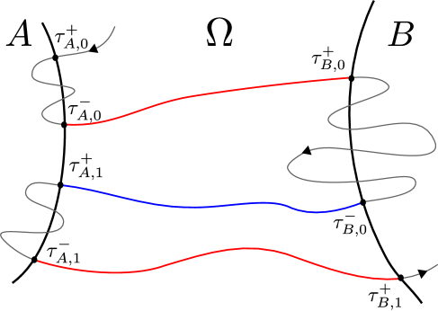
Figure 1. Illustration of a trajectory with entrance and exit times. The transition path from $A$ to $B$ is marked in red.

Our main results describe the probability law of these transition paths in terms of a transition path process, which is a strong solution to an auxiliary stochastic differential equation. In particular, empirical samples of the reactive portions of $X_{t}$ may be regarded as sampling from the transition path process. The motivation comes from the study of chemical reactions and thermally activated processes where understanding these reactive trajectories are crucial [DellagoBolhuisGeissler:02, BolhuisChandlerDellagoGeissler:02]. In these applications, the domains $A$ and $B$ are usually chosen as regions in configurational space corresponding to reactant and product states. Mathematically, our results fit into the framework of the transition path theory [EVa:10, EVa:06, MeScVa:06].

Having identified the transition path process, we can compute statistics of the transition paths by sampling directly from the transition path SDE, rather than using acceptance/rejection methods or very long-time integration on the original SDE. Of course, this assumes knowledge of the committor function, which is non-trivial. In any case, our results might be used to analyze methods of sampling reactive trajectories.

We will now describe our main results and their relation to other works. Proofs are deferred to later sections.

1.1. The transition path process

Our definition of the transition path process is motivated by the Doob $h$-transform as follows. Let $\tau_{A}$ and $\tau_{B}$ denote the first hitting time of $X_{t}$ to the sets $\widebar{A}$ and $\widebar{B}$, respectively:

(1.4) $$\tau_{A} =\inf\left\{t\geq 0\mid X_{t}\in\widebar{A}\right\},$$

$$\tau_{B} =\inf\left\{t\geq 0\mid X_{t}\in\widebar{B}\right\}.$$

Let $q(x)\geq 0$ be the forward committor function:

(1.5) $$q(x)={\mathbb{P}}(\tau_{A}>\tau_{B}\mid X_{0}=x),$$

which satisfies $Lq(x)=0$ for $x\in\Theta=(\widebar{A\cup B})^{C}$ and

(1.6) $$q(x)=\begin{cases}0,&x\in\widebar{A},\\ 1,&x\in\widebar{B}.\end{cases}$$

By the maximum principle, $q(x)>0$ for all $x\in\Theta$. By the Hopf lemma we also have

(1.7) $$\sup_{x\in\partial A}\widehat{n}(x)\cdot\nabla q(x)<0,\qquad\inf_{x\in\partial B}\widehat{n}(x)\cdot\nabla q(x)>0,$$

where $\widehat{n}(x)$ will denote the unit normal exterior to $\Theta$ (pointing into $A$ and $B$). For $x\in\Theta$, consider the stopped process $X_{t\wedge\tau_{A}\wedge\tau_{B}}$ with $X_{0}=x$, and let $\mathcal{P}_{x}$ denote the corresponding measure on $\mathcal{X}=C([0,\infty))$:

$$\mathcal{P}_{x}(U)={\mathbb{P}}(X\in U\;|\;X_{0}=x),\quad\forall\;U\in\mathcal{B}$$

where $\mathcal{B}$ is the Borel $\sigma$-algebra on $\mathcal{X}$. If $\Lambda_{AB}$ denotes the event that $\tau_{A}>\tau_{B}$, the measure $\mathcal{Q}_{x}^{q}$ on $(\mathcal{X},\mathcal{B})$ defined by

$$\dfrac{\mathrm{d}\mathcal{Q}_{x}^{q}}{\mathrm{d}\mathcal{P}_{x}}=\dfrac{\mathbb{I}_{\Lambda_{AB}}}{\mathcal{P}_{x}(\Lambda_{AB})}=\dfrac{\mathbb{I}_{\Lambda_{AB}}}{q(x)}$$

is absolutely continuous with respect to $\mathcal{P}_{x}$, if $x\in\Theta$. By the Doob $h$-transform (see e.g. [Day:92], [Pinsky:95]*Theorem 7.2.2), we know that $\mathcal{Q}_{x}^{q}$ defines a diffusion process $Y_{t}$ on $C([0,\infty))$ with generator:

(1.8) $$L^{q}f=\frac{1}{q}L(qf)=\operatorname{tr}(a\nabla^{2}f)+(b\cdot\nabla f)+\frac{2a\nabla q}{q}\cdot\nabla f=Lf+\frac{2a\nabla q}{q}\cdot\nabla f.$$

So, the effect of conditioning on the event $\tau_{B}<\tau_{A}$ is to introduce an additional drift term.

This observation suggests that the $A\to B$ reactive trajectories should have the same law as a solution to the SDE

(1.9) $$\mathrm{d}Y_{t}=\Bigl{(}b(Y_{t})+\dfrac{2a(Y_{t})\nabla q(Y_{t})}{q(Y_{t})}\Bigr{)}\,\mathrm{d}t+\sqrt{2}\,\sigma(Y_{t})\,\mathrm{d}\widehat{W}_{t},$$

originating at a point $Y_{0}=y_{0}\in\partial A$ and terminating at a point in $\partial B$. While the SDE (1.9) admits strong solutions for $y_{0}\in\Theta$ since $q(x)>0$ in $\Theta$, the drift term becomes singular at the boundary of $A$, where $q$ vanishes. Our first result is the following theorem which shows that there is still a unique strong solution to this SDE even for initial condition lying in $\partial A$. For convenience, let us define the vector field

(1.10) $$K(y)=\Bigl{(}b(y)+\frac{2a(y)\nabla q(y)}{q(y)}\Bigr{)}.$$

Theorem 1.1.

Let $(\widehat{W},\mathcal{F}^{\widehat{W}}_{t})$ be a standard Brownian motion in ${\mathbb{R}}^{d}$, defined on a probability space $(\widehat{\Omega},\widehat{\mathcal{F}},\mathbb{Q})$. Let $\xi:\widehat{\Omega}\to\widebar{\Theta}$ be a random variable defined on the same probability space and independent of $\widehat{W}$. There is a unique, continuous process $Y_{t}:[0,\infty)\to\widebar{\Theta}$ which is adapted to the augmented filtration $\widehat{\mathcal{F}}_{t}$ and satisfying the following, $\mathbb{Q}$-almost surely:

(1.11) $$Y_{t}=\xi+\int_{0}^{t\wedge\tau_{B}}K(Y_{s})\,\mathrm{d}s+\int_{0}^{t\wedge\tau_{B}}\sqrt{2}\,\sigma(Y_{s})\,\mathrm{d}\widehat{W}_{s},\quad t\geq 0$$

where

$$\tau_{B}=\inf\{t>0\mid Y_{t}\in\widebar{B}\}.$$

Moreover, $Y_{t}\not\in\widebar{A}$ for all $t>0$.

The augmented filtration is defined in the usual way, $\widehat{\mathcal{F}}_{t}$ being the $\sigma$-algebra generated by $\mathcal{F}_{t}^{\widehat{W}}$, $Y_{0}$, and the appropriate collection of null sets so that $\widehat{\mathcal{F}}_{t}$ is both left- and right- continuous. We will use $\widehat{\mathbb{E}}$ to denote expectation with respect to the probability measure $\mathbb{Q}$.

Observe that if $d=1$, $\sigma=1/\sqrt{2}$ is constant, and $b\equiv 0$, then $q(x)$ is a linear function, and (1.9) corresponds to a Bessel process of dimension 3. For example, if $A=(-\infty,0)$, $B=(1,\infty)$, we have

$$\mathrm{d}Y_{t}=\frac{1}{Y_{t}}\,\mathrm{d}t+\,\mathrm{d}\widehat{W}_{t},$$

and the function $Z_{t}=(Y_{t})^{2}$ satisfies the degenerate diffusion equation

(1.12) $$\mathrm{d}Z_{t}=3\,\mathrm{d}t+2\sqrt{Z_{t}}\,\mathrm{d}\widehat{W}_{t}.$$

In this simple case, existence and uniqueness of a strong solution starting at $Y_{0}=0$ can be shown using arguments involving Brownian local time (see [ReYo:04, KaSh:91]). However, those arguments are not applicable to the more general setting we consider here. The work most closely related to Theorem 1.1 in a higher dimensional setting may be that of DeBlaissie [Deb:04] who proved pathwise uniqueness for certain SDEs having diffusion coefficients that degenerate like $\sqrt{d(Z_{t})}$ where $d(z)$ is the distance to the domain boundary (as in (1.12)). In an earlier work, Athreya, Barlow, Bass, and Perkins [ABBP:2002] proved uniqueness for the martingale problem associated with a similarly degenerate diffusion in a positive orthant in ${\mathbb{R}}^{d}$. Nevertheless, those analyses do not apply to the case (1.9) considered here.

Our next result is the following theorem which shows that the law of the reactive trajectories is that of the process $Y_{t}$ with appropriate initial condition. For this reason, we will call the process $Y_{t}$ the transition path process.

Theorem 1.2.

Let $X_{t}$ satisfy the SDE (1.1). Let $Y^{k}$ denote the $k^{\text{th}}$ $A\to B$ reactive trajectory defined by (1.3). Let $Y$ be defined as in Theorem 1.1. Then for any bounded and continuous functional $F:C([0,\infty))\to{\mathbb{R}}$, we have

$$\mathbb{E}[F(Y^{k})]=\widehat{\mathbb{E}}\left[F(Y)\mid Y_{0}\sim X_{\tau_{A,k}^{-}}\right].$$

The processes $X_{t}$ and $Y^{k}_{t}$ are defined on a probability space that is different from the one on which $Y_{t}$ is defined. The notation $Y_{0}\sim X_{\tau_{A,k}^{-}}$ used in Theorem 1.2 means that $Y_{0}$ has the same law as $X_{\tau_{A,k}^{-}}$, meaning $\mathbb{Q}(Y_{0}\in U)={\mathbb{P}}(X_{\tau_{A,k}^{-}}\in U)$ for any Borel set $U\subset{\mathbb{R}}^{d}$.

1.2. Reactive exit and entrance distributions

The distribution of the random points $X_{\tau_{A,k}^{-}}$ will depend in the initial condition $X_{0}$. From the point of view of sampling the transition paths, however, there is a very natural distribution to consider for $Y_{0}$. To motivate this distribution formally, let $h>0$ and consider the regularized hitting times

(1.13) $$\tau_{A,h} =\inf\left\{t\geq h\mid X_{t}\in\widebar{A}\right\}$$

(1.14) $$\tau_{B,h} =\inf\left\{t\geq h\mid X_{t}\in\widebar{B}\right\},$$

where $X_{t}$ satisfies (1.1). Then define

$$q_{h}(x)={\mathbb{P}}(\tau_{A,h}>\tau_{B,h}\mid X_{0}=x).$$

This is the probability that at some time $s\in[0,h]$, the path $X_{t}$ starting from $x\in\partial A$ becomes a transition path, not returning to $\bar{A}$ before hitting $\bar{B}$. With this in mind, the quantity

$$\eta_{A,h}(x)=h^{-1}\rho(x){\mathbb{P}}(\tau_{A,h}>\tau_{B,h}\mid X_{0}=x)=h^{-1}\rho(x)q_{h}(x),$$

may be interpreted as a rate at which transition paths exit $A$, when the system is in equilibrium. Therefore, a natural choice for an initial distribution for $Y_{0}\in\partial A$ is:

$$\eta_{A}(x)=\lim_{h\to 0}\eta_{A,h}.$$

By the Markov property, we have

(1.15) $$q_{h}(x)=\int_{{\mathbb{R}}^{d}}{\mathbb{P}}(\tau_{A}>\tau_{B}\;|\;X_{0}=y)\rho(h,x,y)\,\mathrm{d}y=\mathbb{E}[q(X_{h})\mid X_{0}=x]$$

where $\rho(t,x,\cdot)$ is the density for $X_{t}$, given $X_{0}=x$. Therefore, for any $x\in\partial A$ we have

$$\lim_{h\to 0}h^{-1}q_{h}(x)=\lim_{h\to 0}h^{-1}\mathbb{E}[q(X_{h})-q(X_{0})\;|\;X_{0}=x]=Lq(x),$$

in the sense of distributions, although $q$ is not $C^{2}$ on $\partial\Theta=\partial A\cup\partial B$. Hence $\eta_{A,h}(x)\to\eta_{A}(x)=\rho(x)Lq(x)$ for $x\in\partial A$. The distribution $Lq$ is supported on $\partial\Theta$. If $\phi$ is a smooth test function supported on a set $B_{r}(x)$, a small neighborhood of $x\in\partial A$, then we have

$$\langle Lq,\phi\rangle =\int_{{\mathbb{R}}^{d}}q(x)L^{\ast}\phi(x)\,\mathrm{d}x$$

$$=\int_{B_{r}(x)\cap\Theta}Lq(x)\phi(x)\,\mathrm{d}x+\int_{(\partial A)\cap B_{r}(x)}\bigl{(}q\widehat{n}\cdot\operatorname{div}(a\phi)-(\widehat{n}\cdot a\nabla q)\phi+q\widehat{n}\cdot b\,\phi\bigr{)}\,\mathrm{d}\sigma_{A}(x)$$

where $\widehat{n}(x)$ is the unit normal vector exterior to $\Theta$, and $\,\mathrm{d}\sigma_{A}$ is the surface measure on $\partial A$. Since $q=0$ on $\partial A$ and $Lq=0$ on $\Theta$, this implies,

$$\langle Lq,\phi\rangle=-\int_{(\partial A)\cap B_{r}(x)}\phi\,\widehat{n}\cdot a\nabla q\,\mathrm{d}\sigma_{A}(x).$$

That is (after a similar calculation for points on $\partial B$),

(1.16) $$Lq(x)=-\widehat{n}(x)\cdot a(x)\nabla q(x)\,\mathrm{d}\sigma_{A}(x)-\widehat{n}(x)\cdot a(x)\nabla q(x)\,\mathrm{d}\sigma_{B}(x),$$

in the sense of distributions. Restricting on $\partial A$, we get

(1.17) $$\eta_{A}=-\rho(x)\widehat{n}(x)\cdot a(x)\nabla q(x)\,\mathrm{d}\sigma_{A}(x).$$

By switching the role of $A$ and $B$ in the above discussion, it is also natural to define a measure on $\partial B$ as

(1.18) $$\eta_{B}=\rho(x)\widehat{n}(x)\cdot a(x)\nabla q(x)\,\mathrm{d}\sigma_{B}(x).$$

Note that $1-q$ gives the forward committor function for the transition from $B$ to $A$ and that $Lq(x)=\eta_{A}(\mathrm{d}x)-\eta_{B}(\mathrm{d}x)$. Although the distributions $\eta_{A}$ and $\eta_{B}$ are positive (by (1.7)), they need not be probability distributions. Nevertheless, the mass of the two measures is the same.

Lemma 1.3.

The measures $\eta_{A}$ and $\eta_{B}$ satisfy $\eta_{A}(\partial A)=\eta_{B}(\partial B)$. That is,

(1.19) $$\int_{\partial A}\rho(x)\widehat{n}(x)\cdot a(x)\nabla q(x)\,\mathrm{d}\sigma_{A}(x)+\int_{\partial B}\rho(x)\widehat{n}(x)\cdot a(x)\nabla q(x)\,\mathrm{d}\sigma_{B}(x)=0.$$

This computation motivates us to define

(1.20) $$\eta_{A}^{-}(\mathrm{d}x)=\frac{1}{\nu}\eta_{A}(\mathrm{d}x)=-\frac{1}{\nu}\rho(x)\widehat{n}(x)\cdot a(x)\nabla q(x)\,\mathrm{d}\sigma_{A}(x),$$

(1.21) $$\eta_{B}^{-}(\mathrm{d}x)=\frac{1}{\nu}\eta_{B}(\mathrm{d}x)=\frac{1}{\nu}\rho(x)\widehat{n}(x)\cdot a(x)\nabla q(x)\,\mathrm{d}\sigma_{B}(x),$$

We call these distributions the reactive exit distribution on $\partial A$ and on $\partial B$, respectively. The constant $\nu$ is a normalizing constant so that $\eta_{A}^{-}$ and $\eta_{B}^{-}$ define probability measures on $\partial A$ and $\partial B$. By Lemma 1.3, the normalizing constant is the same for both measures. Our next result relates the reactive exit distribution on $\partial A$ to the empirical reactive exit distribution on $\partial A$, defined by

(1.22) $$\mu_{A,N}^{-}=\frac{1}{N}\sum_{k=0}^{N-1}\delta_{X_{\tau_{A,k}^{-}}}(x).$$

Proposition 1.4.

Let $\mu_{A,N}^{-}$ be the empirical reactive exit distribution on $\partial A$ defined by (1.22). Then $\mu_{A,N}^{-}$ converges weakly to $\eta_{A}^{-}$ as $N\to\infty$. That is, for any continuous and bounded $f:\partial A\to{\mathbb{R}}$

$$\lim_{N\to\infty}\int_{\partial A}f(x)\,\mathrm{d}\mu_{A,N}^{-}(x)=\int_{\partial A}f(x)\,\mathrm{d}\eta_{A}^{-}(x)$$

holds ${\mathbb{P}}$-almost surely.

A similar statement holds for the reactive exit distribution on $\partial B$ and the empirical distribution of the points $X_{\tau_{B,k}^{-}}$. The reactive exit distribution $\eta_{A}^{-}(\mathrm{d}x)$ is related to the equilibrium measure $e_{A,B}(\mathrm{d}x)$ in the potential theory for diffusion processes [Sznitman:98, BoEcGaKl:04, BoGaKl:05]. In fact, the committor function $q$ is known as the equilibrium potential in those works, and the equilibrium measure $e_{A,B}(\mathrm{d}x)$ is given by $Lq$ restricted on $\partial A$. Specifically, we have

(1.23) $$\eta_{A}^{-}(\mathrm{d}x)=\frac{1}{\nu}\rho(x)e_{A,B}(\mathrm{d}x).$$

To the best of our knowledge, Proposition 1.4 for the first time characterizes the equilibrium measure from a dynamic perspective.

We also identify the limit of the empirical reactive entrance distribution on $\partial B$, defined as

(1.24) $$\mu_{B,N}^{+}=\frac{1}{N}\sum_{k=0}^{N-1}\delta_{X_{\tau_{B,k}^{+}}}(x).$$

To describe its limit as $N\to\infty$, let us denote by $\widetilde{L}$ the adjoint of $L$ in $L^{2}({\mathbb{R}}^{d},\rho(x)\mathrm{d}x)$, given by

(1.25) $$\widetilde{L}u=-b\cdot\nabla u+\frac{2}{\rho}\operatorname{div}(a\rho)\cdot\nabla u+\operatorname{tr}(a\nabla^{2}u).$$

This corresponds to the generator of the time-reversed process $t\mapsto X_{T-t}$ [HaussmannPardoux:86]. Note that $\widetilde{L}=L$ if the SDE (1.1) is reversible, i.e. $L$ is self-adjoint in $L^{2}({\mathbb{R}}^{d},\rho(x)\,\mathrm{d}x)$. In addition to the forward committor function $q(x)$ (recall (1.5)), we also define the backward committor function $\widetilde{q}(x)$ to be the unique solution of

$$\widetilde{L}\widetilde{q}=0,\quad x\in\Theta$$

with boundary condition

$$\widetilde{q}(x)=\begin{cases}1,&x\in\partial A\\ 0,&x\in\partial B.\end{cases}$$

In terms of $\widetilde{q}$, we define the reactive entrance distribution on $\partial B$ as

(1.26) $$\eta_{B}^{+}(\mathrm{d}x)=-\frac{1}{\nu}\rho(x)\widehat{n}(x)\cdot a(x)\nabla\widetilde{q}(x)\,\mathrm{d}\sigma_{B}(x)$$

and analogously the reactive entrance distribution on $\partial A$

(1.27) $$\eta_{A}^{+}(\mathrm{d}x)=\frac{1}{\nu}\rho(x)\widehat{n}(x)\cdot a(x)\nabla\widetilde{q}(x)\,\mathrm{d}\sigma_{A}(x).$$

Again, $\nu$ is a normalizing constant so that these are probability measures; $\nu$ is the same as the constant in (1.20). The following proposition justifies the definition of the reactive entrance distribution.

Proposition 1.5.

Let $\mu_{B,N}^{+}$ be the empirical reactive entrance distribution on $\partial B$ defined by (1.24). Then $\mu_{B,N}^{+}$ converges weakly to $\eta_{B}^{+}$ as $N\to\infty$. That is, for any continuous and bounded $f:\partial B\to{\mathbb{R}}$

$$\lim_{N\to\infty}\int_{\partial B}f(x)\,\mathrm{d}\mu_{B,N}^{+}(x)=\int_{\partial B}f(x)\,\mathrm{d}\eta_{B}^{+}(x)$$

holds ${\mathbb{P}}$-almost surely.

A similar statement holds for the reactive entrance distribution on $\partial A$ and the empirical distribution of the points $X_{\tau_{A,k}^{+}}$.

Remark 1.6.

If the SDE (1.1) is reversible, we have $\widetilde{q}=1-q$, and hence $\eta_{A}^{+}(\mathrm{d}x)=\eta_{A}^{-}(\mathrm{d}x)$ and $\eta_{B}^{+}(\mathrm{d}x)=\eta_{B}^{-}(\mathrm{d}x)$.

In view of Proposition 1.4, $\eta_{A}^{-}$ is a natural choice for the distribution of $Y_{0}$. With this choice, the transition path process $Y_{t}$ characterizes the empirical distribution of $A\to B$ reactive trajectories, as the next theorem shows:

Theorem 1.7.

Let $X_{t}$ satisfy the SDE (1.1). Let $Y^{k}$ denote the $k^{\text{th}}$ $A\to B$ reactive trajectory defined by (1.3). Let $Y$ be the unique process defined by Theorem 1.1 with initial distribution $Y_{0}\sim\eta_{A}^{-}(\mathrm{d}x)$ on $\partial A$ defined by (1.20), and let $\mathcal{Q}_{\eta_{A}^{-}}$ denote the law of this process on $\mathcal{X}=C([0,\infty))$. Then for any $F\in L^{1}(\mathcal{X},\mathcal{B},\mathcal{Q}_{\eta_{A}^{-}})$, the limit

$$\lim_{N\to\infty}\frac{1}{N}\sum_{k=0}^{N-1}F(Y^{k})=\widehat{\mathbb{E}}[F(Y)]$$

holds ${\mathbb{P}}$-almost surely.

In particular, the limit $\widehat{\mathbb{E}}[F(Y)]$ is independent of $X_{0}$. Using Theorem 1.7, several interesting statistics of the transition paths can be expressed in terms of the quantities we have defined. Actually, Proposition 1.4 is an immediate corollary of Theorem 1.7, by choosing $F(Y^{k})=f(Y^{k}_{0})$, so we will not give a separate proof of Proposition 1.4.

1.3. Reaction rate

Let $N_{T}$ be the number of $A\to B$ reactive trajectories up to time $T$:

$$N_{T}=1+\max_{k}\{k\geq 0\mid\tau_{B,k}^{+}\leq T\}.$$

The reaction rate $\nu_{R}$ is defined by the limit

(1.28) $$\nu_{R}=\lim_{T\to\infty}\frac{N_{T}}{T}=\lim_{k\to\infty}\frac{k}{\tau_{B,k}^{+}},$$

and it is the rate of the transition from $A$ to $B$. Also, the limits

(1.29) $$T_{AB}:=\lim_{N\to\infty}\frac{1}{N}\sum_{k=0}^{N-1}(\tau_{B,k}^{+}-\tau_{A,k}^{+})$$

and

(1.30) $$T_{BA}:=\lim_{N\to\infty}\frac{1}{N}\sum_{k=0}^{N-1}(\tau_{A,k+1}^{+}-\tau_{B,k}^{+})$$

are the expected reaction times from $A\to B$ and $B\to A$, respectively. The reaction rate from $A\to B$ and $B\to A$ are then given by $k_{AB}=T_{AB}^{-1}$ and $k_{BA}=T_{BA}^{-1}$. Another interesting quantity is the expected crossover time from $A\to B$

(1.31) $$C_{AB}:=\lim_{N\to\infty}\frac{1}{N}\sum_{k=0}^{N-1}(\tau_{B,k}^{+}-\tau_{A,k}^{-}),$$

which is the typical duration of the $A\to B$ reactive intervals. Observe that $C_{AB}<T_{AB}$. Similarly, we define

(1.32) $$C_{BA}:=\lim_{N\to\infty}\frac{1}{N}\sum_{k=0}^{N-1}(\tau_{A,k+1}^{+}-\tau_{B,k}^{-}).$$

The next result identifies these limits in terms of the committor functions and the reactive exit and entrance distributions.

Proposition 1.8.

The limits (1.28), (1.29), (1.30), (1.31), and (1.32) hold ${\mathbb{P}}$-almost surely, and

$$\nu_{R}=\nu=\int_{\mathbb{R}^{d}}\rho(x)\nabla q(x)\cdot a(x)\nabla q(x)\,\mathrm{d}x.$$

$$T_{AB}=\int_{\partial A}\eta_{A}^{+}(\mathrm{d}x)u_{B}(x)=\frac{1}{\nu_{R}}\int_{\mathbb{R}^{d}}\rho(x)\widetilde{q}(x)\,\mathrm{d}x.$$

$$T_{BA}=\int_{\partial B}\eta_{B}^{+}(\mathrm{d}x)u_{A}(x)=\frac{1}{\nu_{R}}\int_{\mathbb{R}^{d}}\rho(x)(1-\widetilde{q}(x))\,\mathrm{d}x.$$

$$C_{AB}=\int_{\partial A}\eta_{A}^{-}(\mathrm{d}x)v_{B}(x)=\frac{1}{\nu_{R}}\int_{\mathbb{R}^{d}}\rho(x)q(x)\widetilde{q}(x)\,\mathrm{d}x.$$

$$C_{BA}=\int_{\partial B}\eta_{B}^{-}(\mathrm{d}x)v_{A}(x)=\frac{1}{\nu_{R}}\int_{\mathbb{R}^{d}}\rho(x)(1-q(x))(1-\widetilde{q}(x))\,\mathrm{d}x.$$

Here $u_{B}(x)=\mathbb{E}[\tau^{X}_{B}\;|\;X_{0}=x]$ is the mean first hitting time of $X_{t}$ to $\widebar{B}$, and $v_{B}(x)=\widehat{\mathbb{E}}[\tau^{Y}_{B}\;|\;Y_{0}=x]$ is the mean first hitting time of $Y_{t}$ to $\widebar{B}$. Similarly, if $q$ is replaced by $(1-q)$ in the definition of $Y$, then $v_{A}(x)=\widehat{\mathbb{E}}[\tau^{Y}_{A}\;|\;Y_{0}=x]$. Recall that $\nu$ is the normalizing factor for the reactive exit and entrance distributions.

The formula for $\nu_{R}$, $T_{AB}$, and $T_{BA}$ were obtained in [EVa:06]. We also note that the crossover time for the transition path process in one dimension was recently studied by [Cerou:12].

1.4. Density of transition paths

We now consider the distribution $\rho_{R}$ as defined in [EVa:06]:

(1.33) $$\rho_{R}(z)=\lim_{T\to\infty}\frac{1}{T}\int_{0}^{T}\delta(z-X_{t})\mathbb{I}_{R}(t)\,\mathrm{d}t,\quad z\in\Theta,$$

where $R$ is the random set of times at which $X_{t}$ is reactive:

$$R=\bigcup_{k=0}^{\infty}[\tau_{A,k}^{-},\tau_{B,k}^{+}].$$

This distribution on $\Theta$ can be viewed as the density of transition paths. By Proposition 1.8, and Theorem 1.7, we can describe $\rho_{R}$ in terms of the transition density for $Y_{t}$. Specifically, for any continuous and bounded function $f:{\mathbb{R}}^{d}\to{\mathbb{R}}$, we have

$$\int_{\Theta}f(z)\rho_{R}(z)\,\mathrm{d}z =\nu_{R}\lim_{T\to\infty}\frac{1}{N_{T}}\int_{0}^{T}f(X_{t})\mathbb{I}_{R}(t)\,\mathrm{d}t$$

$$=\nu_{R}\lim_{N\to\infty}\frac{1}{N}\sum_{k=0}^{N-1}\int_{0}^{\tau_{B,k}^{+}-\tau_{A,k}^{-}}f\bigl{(}Y^{k}_{t}\bigr{)}\,\mathrm{d}t$$

$$=\nu_{R}\,\widehat{\mathbb{E}}\left[\int_{0}^{t_{B}}f(Y_{t})\,\mathrm{d}t\mid Y_{0}\sim\eta_{A}^{-}\right]$$

$$=\nu_{R}\int_{0}^{\infty}\int_{\Theta}Q_{R}(t,\eta_{A}^{-},z)f(z)\,\mathrm{d}z\,\,\mathrm{d}t.$$

Here $Q_{R}(t,\eta_{A}^{-},z)$ is the density of $Y_{t}$, with $Y_{0}\sim\eta_{A}^{-}$, and killed at $\partial B$

(1.34) $$Q_{R}(t,\eta_{A}^{-},z)=\mathbb{Q}(Y_{t}\in\mathrm{d}z,\,t<t_{B}\mid Y_{0}\sim\eta_{A}^{-}),$$

and $t_{B}$ is the first hitting time of $Y_{t}$ to $\widebar{B}$. Hence, for $z\in\Theta$,

(1.35) $$\rho_{R}(z) =\nu_{R}\int_{0}^{\infty}Q_{R}(t,\eta_{A}^{-},z)\,\mathrm{d}t.$$

Proposition 1.9.

For all $z\in\Theta$,

(1.36) $$\rho_{R}(z)=\rho(z)q(z)\widetilde{q}(z).$$

This formula for $\rho_{R}$ was first derived in [Hummer:04, EVa:06].

1.5. Current of transition paths

The density $Q_{R}(t,\eta_{A}^{-},z)$ satisfies the adjoint equation

$$\frac{\partial}{\partial t}Q_{R}(t,\eta_{A}^{-},z)=(L^{q})^{\ast}Q_{R}(t,\eta_{A}^{-},z),\quad z\in\Theta$$

where $(L^{q})^{\ast}$ is the adjoint of $L^{q}$:

$$(L^{q})^{\ast}u=\sum_{i,j}(a_{ij}(z)u(z))_{z_{i}z_{j}}-\sum_{i}(K_{i}(z)u(z))_{z_{i}}$$

and $K$ is defined by (1.10). Integrating from $t=0$ to $t=\infty$ we see that $\rho_{R}(z)$ satisfies

$$(L^{q})^{\ast}\rho_{R}(z)=0,\quad z\in\Theta.$$

In divergence form, this equation is

(1.37) $$\nabla_{z}\cdot J_{R}(z)=0,$$

where the vector field

(1.38) $$J_{R}(z) =\rho_{R}(z)\biggl{(}b(z)-\frac{2a\nabla q(z)}{q(z)}\biggr{)}+\operatorname{div}(a(z)\rho_{R}(z))$$

$$=\Bigl{(}b(z)\rho(z)-\operatorname{div}\bigl{(}a(z)\rho(z)\bigr{)}\Bigr{)}q(z)\widetilde{q}(z)+\rho(z)a(z)\Bigl{(}\widetilde{q}(z)\nabla q(z)-q(z)\nabla\widetilde{q}(z)\Bigr{)}.$$

is continuous over $\widebar{\Theta}$. The vector field $J_{R}(z)$, identified in [EVa:06], may be regarded as the current of transition paths (see Remark 1.13). Observe that if the SDE (1.1) is reversible, we have $\widetilde{q}=1-q$ and

$$b(z)\rho(z)-\operatorname{div}(a(z)\rho(z))=0,$$

and hence the current given by (1.38) simplifies to

$$J_{R}(z)=\rho(z)a(z)\nabla q(z).$$

This was observed already in [EVa:06].

On the boundary, the current (1.38) is related to the reactive exit and entrance distributions.

Proposition 1.10.

We have

$$J_{R}=\rho a\nabla q\;\text{on }\partial A,\quad\text{and}\quad J_{R}=-\rho a\nabla\widetilde{q},\;\text{on }\partial B,$$

and hence,

$$\eta_{A}^{-}(\mathrm{d}x)=-\nu_{R}^{-1}\widehat{n}(x)\cdot J_{R}(x)\,\mathrm{d}\sigma_{A}(x)\quad\text{and}\quad\eta_{B}^{+}(\mathrm{d}x)=\nu_{R}^{-1}\widehat{n}(x)\cdot J_{R}(x)\,\mathrm{d}\sigma_{B}(x).$$

As an immediate corollary, we have an additional formula for the reaction rate.

Corollary 1.11.

Let $S$ be a set with smooth boundary that contains $A$ and separates $A$ and $B$, we have

(1.39) $$\nu_{R}=\int_{\partial S}\widehat{n}(x)\cdot J_{R}(x)\,\mathrm{d}\sigma_{S}(x),$$

where $\widehat{n}$ is the unit normal vector exterior to $S$.

The current $J_{R}$ generates a (deterministic) flow in $\widebar{\Theta}$ stopped at $\partial B$:

(1.40) $$\frac{\,\mathrm{d}Z_{t}^{z}}{\,\mathrm{d}t}=J_{R}(Z_{t}^{z}),\quad\text{for }0\leq t\leq t_{B},\quad Z_{0}^{z}=z$$

where $t_{B}=t_{B}(z)$ is the time at which $Z_{t}$ reaches $\partial B$. As $J_{R}$ is divergence free in $\Theta$, $J_{R}\cdot\widehat{n}<0$ on $\partial A$, and $J_{R}\cdot\widehat{n}>0$ on $\partial B$, $t_{B}(z)$ is finite for any $z\in\widebar{\Theta}$. The flow naturally defines a map $\Phi_{J_{R}}:\partial A\to\partial B$: given any point $z\in\partial A$, we define

(1.41) $$\Phi_{J_{R}}(z)=Z_{t_{B}}^{z}\in\partial B.$$

Proposition 1.12.

For any $f\in C^{1}({\mathbb{R}}^{d})$,

(1.42) $$\int_{\partial B}f(x)\eta_{B}^{+}(\mathrm{d}x)-\int_{\partial A}f(x)\eta_{A}^{-}(\mathrm{d}x)=\frac{1}{\nu_{R}}\int_{\Theta}J_{R}\cdot\nabla f\,\mathrm{d}x.$$

In particular,

$$\Phi_{J_{R},\ast}(\eta_{A}^{-})=\eta_{B}^{+},$$

where $\Phi_{J_{R},\ast}(\eta_{A}^{-})$ is the pushforward of the measure $\eta_{A}^{-}$ by the map $\Phi_{J_{R}}$.

Hence, $J_{R}$ characterizes “the flow of reactive trajectories” from $A$ to $B$.

Remark 1.13.

Note that by Proposition 1.4 and Proposition 1.5, the left hand side of (1.42) is equal, ${\mathbb{P}}$-almost surely, to the limit

$$\lim_{N\to\infty}\frac{1}{N}\sum_{n=0}^{N-1}\bigl{(}f(X_{\tau_{B,n}^{+}})-f(X_{\tau_{A,n}^{-}})\bigr{)}.$$

If $X_{t}$ was differentiable, we would have

$$\lim_{N\to\infty}\frac{1}{N}\sum_{n=0}^{N-1}\Bigl{(}f(X_{\tau_{B,n}^{+}})-f(X_{\tau_{A,n}^{-}})\Bigr{)} =\lim_{T\to\infty}\frac{1}{\nu_{R}}\frac{1}{T}\int_{0}^{T}1_{R}(t)\frac{\mathrm{d}}{\mathrm{d}t}f(X_{t})\,\mathrm{d}t$$

$$\text{``}=\frac{1}{\nu_{R}}\int_{\Theta}\,\mathrm{d}x\nabla f(x)\cdot\lim_{T\to\infty}\frac{1}{T}\int_{0}^{T}\dot{X}_{t}\delta(x-X_{t})1_{R}(t)\,\mathrm{d}t\ \text{''},$$

Combining this with Proposition 1.12, we arrive at a formal characterization of $J_{R}$

$$J_{R}\text{``}=\lim_{T\to\infty}\frac{1}{T}\int_{0}^{T}\dot{X}_{t}\delta(x-X_{t})1_{R}(t)\,\mathrm{d}t\ \text{''}.$$

This formal expression was used in [EVa:06] to define $J_{R}$.

1.6. Related work

As we have mentioned, our work is closely related to the transition path theory developed by E and Vanden-Eijnden [EVa:06, MeScVa:06, EVa:10], which is a framework for studying the transition paths. In particular, based on the committor function, formula for reaction rate, density and current of transition paths were obtained in [EVa:06]. Our main motivation is to understand the probability law of the transition paths. The main results Theorem 1.1, Theorem 1.2, and Theorem 1.7 identify an SDE which characterizes the law of the transition paths in $C([0,\infty))$. Therefore, as an application of these results, we are able to give rigorous proofs for the formula for reaction rate, density and current of transition paths in [EVa:06]. We note that in the discrete case, a generator analogous to (1.8) was also proposed very recently in [EricPreprint] for Markov jumping processes.

The transition paths start at $\partial A$ and terminate at $\partial B$, and hence they can be viewed as paths of a bridge process between $\widebar{A}$ and $\widebar{B}$. In this perspective, our work is related to the conditional path sampling for SDEs studied in [StuartVossWiberg:04, ReznikoffVandenEijnden:05, HairerStuartVossWiberg:05, HairerStuartVoss:07]. In those works, stochastic partial differential equations were proposed to sample SDE paths with fixed end points. However, the paths considered were different from the transition paths as their time duration is fixed a priori. It would be interesting to explore SPDE-based sampling strategies for the transition path process identified in Theorem 1.1.

Let us also point out that in the work we present here we do not assume that the noise $\sigma$ is small, as is the case in the asymptotic results of [BoEcGaKl:04, BoGaKl:05, Cerou:12], which we have mentioned already, and also in some other works, such as the large deviation theory of Freidlin and Wentzell [FW:84].

The rest of the paper is organized as follows. Theorem 1.1 and Theorem 1.2 are proved in Section 2. In Section 3 we prove Lemma 1.3, Proposition 1.5 and Theorem 1.7 related to the reactive entrance and exit distributions. As we have mentioned, Proposition 1.4 follows immediately from Theorem 1.7, so we do not give a separate proof of it. Proposition 1.8, Proposition 1.9, Proposition 1.10, Corollary 1.11, and Proposition 1.12 are proved in Section 4.

2. The Transition Path Process

Proof of Theorem 1.1.

Without loss of generality, we prove the theorem in the case that $\xi\equiv y_{0}$ is a single point in $\widebar{\Theta}$. The interesting aspect of the theorem is that $y_{0}$ is allowed to be on $\partial\Theta$, since the drift term is singular at $\partial\Theta$. If we assume that $y_{0}\in\Theta$, then existence of a unique strong solution up to the time $\tau_{A}\wedge\tau_{B}$ follows from standard arguments, since $K(y)$ is Lipschitz continuous in the interior of $\Theta$. That is, if $y_{0}\in\Theta$, there is a unique, continuous $\widehat{\mathcal{F}}_{t}$-adapted process $Y_{t}$ which satisfies

(2.1) $$Y_{t}=y_{0}+\int_{0}^{t\wedge(\tau_{A}\wedge\tau_{B})}K(Y_{s})\,\mathrm{d}s+\int_{0}^{t\wedge(\tau_{A}\wedge\tau_{B})}\sqrt{2}\,\sigma(Y_{s})\,\mathrm{d}\widehat{W}_{s},\quad t\geq 0.$$

Moreover, if $y_{0}\in\Theta$, then we must have $\tau_{A}>\tau_{B}>0$ almost surely. This follows from an argument similar to the proof of [KaSh:91]*Proposition 3.3.22, p. 161. Specifically, we consider the process $z_{t}=1/q(Y_{t})\in{\mathbb{R}}$, which satisfies

$$z_{t\wedge\tau}=z_{0}-\int_{0}^{t\wedge\tau}\sqrt{2}(z_{s})^{2}\nabla q\cdot\sigma\,\mathrm{d}\widehat{W}_{s}$$

where $\tau=\tau_{B}\wedge\tau_{\epsilon}$ with $\tau_{\epsilon}=\inf\{t>0\mid q(Y_{t})=\epsilon\}$. Since $\tau<\infty$ with probability one, we have

$$z_{0}=\widehat{\mathbb{E}}[z_{t\wedge\tau}]=\frac{1}{q(\epsilon)}\mathbb{Q}(\tau_{\epsilon}<\tau_{B})+\mathbb{Q}(\tau_{\epsilon}>\tau_{B}).$$

Hence $\mathbb{Q}(\tau_{\epsilon}<\tau_{B})\leq q(\epsilon)(z_{0}-1)$. So, $\mathbb{Q}(\tau_{A}<\tau_{B})\leq\lim_{\epsilon\to 0}\mathbb{Q}(\tau_{\epsilon}<\tau_{B})=0$.

Now suppose $y_{0}\in\partial A$. In consideration of the comments above, it suffices to prove the desired result with $\tau_{B}$ replaced by $\tau_{r}$, the first hitting time to $\partial B_{r}(y_{0})\cap\Theta$, where $B_{r}(y_{0})$ is a ball of radius $r>0$ centered at $y_{0}$. Thus, we want to prove existence and pathwise uniqueness of a continuous $\widehat{\mathcal{F}}_{t}$-adapted process $Y_{t}:[0,\infty)\to\bar{\Theta}$ satisfying

(2.2) $$Y_{t}=y_{0}+\int_{0}^{t\wedge\tau_{r}}K(Y_{s})\,\mathrm{d}s+\int_{0}^{t\wedge\tau_{r}}\sqrt{2}\,\sigma(Y_{s})\,\mathrm{d}\widehat{W}_{s},$$

where

$$\tau_{r}=\inf\left\{t\geq 0\mid Y_{t}\in\partial B_{r}(y_{0})\cap\Theta\,\right\}.$$

It will be very useful to define a new coordinate system in the set $B_{r}^{+}(y_{0})=B_{r}(y_{0})\cap\Theta$ and to consider the problem in these new coordinates. For $r>0$ small enough we can define a $C^{3}$ map $(h^{(1)}(y),\dots,h^{(d-1)}(y),q(y)):\overline{B_{r}^{+}(y_{0})}\to{\mathbb{R}}^{d-1}\times[0,\infty)$, such that the scalar functions $h^{(i)}(y):\overline{B_{r}^{+}(y_{0})}\to{\mathbb{R}}$ satisfy

(2.3) $$\langle\nabla h^{(i)}(y),a(y)\nabla q(y)\rangle=0,\quad\forall\;y\in\overline{B_{r}^{+}(y_{0})},\qquad i=1,\dots,d-1.$$

Furthermore, the map may be constructed so that it is invertible on its range and that the inverse is $C^{3}$. The existence of such a map follows from the regularity of $\partial A$, the regularity of $q$, and the fact that $\langle\widehat{n},a\nabla q\rangle\neq 0$ on $\partial A$ by (1.7).

For two initial points $x_{1},x_{2}\in\Theta$, let $Y^{x_{1}}_{t}$ and $Y^{x_{2}}_{t}$ denote the unique solutions to (2.1) with $Y^{x_{1}}_{0}=x_{1}$ and $Y^{x_{2}}_{0}=x_{2}$ respectively. That is,

(2.4) $$Y^{x}_{t}=x+\int_{0}^{t\wedge\tau^{x}_{B}}K(Y^{x}_{s})\,\mathrm{d}s+\int_{0}^{t\wedge\tau^{x}_{B}}\sqrt{2}\,\sigma(Y^{x}_{s})\,\mathrm{d}\widehat{W}_{s},\quad t\geq 0,$$

where $\tau_{B}^{x}$ is the first hitting time of $Y^{x}_{t}$ to $\partial B$. Changing to the coordinate system defined by $(h^{(1)}(y),\dots,h^{(d-1)}(y),q(y))$, we denote

$$(h_{1,t},q_{1,t})=(h(Y^{x_{1}}_{t}),q(Y^{x_{1}}_{t}))\quad\text{and}\quad(h_{2,t},q_{2,t})=(h(Y^{x_{2}}_{t}),q(Y^{x_{2}}_{t})).$$

Let $\tau_{r}^{1}$ and $\tau_{r}^{2}$ denote the first hitting times of $Y^{x_{1}}_{t}$ and $Y^{x_{2}}_{t}$ to the set $\partial B_{r}(y_{0})\cap\Theta$. The processes $(h_{1,t},q_{1,t})$ and $(h_{2,t},q_{2,t})$ are well-defined up to the times $\tau^{1}_{r}$ and $\tau^{2}_{r}$, respectively.

We can control the difference between $(h_{1,t},q_{1,t})$ and $(h_{2,t},q_{2,t})$:

Lemma 2.1.

There is a constant $C$ such that for all $x_{1},x_{2}\in B_{r/2}(y_{0})\cap\Theta$

$$\widehat{\mathbb{E}}\left[\max_{t\in[0,T]}(q_{1,t\wedge\tau}-q_{2,t\wedge\tau})^{2}\right]\leq C|x_{1}-x_{2}|^{1/2},$$

and

$$\widehat{\mathbb{E}}\left[\max_{t\in[0,T]}\lvert h_{1,t\wedge\tau}-h_{2,t\wedge\tau}\rvert^{2}\right]\leq C|x_{1}-x_{2}|,$$

where $\tau=\tau^{1}_{r}\wedge\tau^{2}_{r}$.

The proof of Lemma 2.1 will be postponed. One immediate corollary is the following.

Corollary 2.2.

There is a constant $C$ such that for all $x_{1},x_{2}\in B_{r/2}(y_{0})\cap\Theta$

(2.5) $$\mathbb{Q}\biggl{(}\max_{0\leq t\leq(T\wedge\tau)}|Y^{x_{1}}_{t}-Y^{x_{2}}_{t}|>\alpha\biggr{)}\leq C\alpha^{-2}|x_{1}-x_{2}|^{1/2},\quad\forall\;\alpha>0,$$

where $\tau=\tau^{1}_{r}\wedge\tau^{2}_{r}$.

Proof.

On the closed set $\{z\in{\mathbb{R}}^{d}\mid z=(h(y),q(y)),\ y\in\overline{B_{r}^{+}(y_{0})}\}$, the map $y\mapsto(h(y),q(y))$ is invertible with a continuously differentiable inverse. Hence there is a constant $C$, depending only on the map $y\mapsto(h(y),q(y))$ such that

$$|Y^{x_{1}}_{t}-Y^{x_{2}}_{t}|\leq C\left(|h_{1,t}-h_{2,t}|+|q_{1,t}-q_{2,t}|\right),\quad\forall\;t\in[0,\tau].$$

By combining this bound with Chebychev’s inequality and Lemma 2.1 we obtain (2.5). ∎

Now suppose $y_{0}\in\partial A$. Let $\{x_{n}\}_{n=1}^{\infty}\subset\Theta$ be a given sequence such that $x_{n}\to y_{0}$ as $n\to\infty$. For each $n$, define $Y^{x_{n}}_{t}$ by (2.4), and let $\tau^{n}_{r}$ denote the first hitting time of $Y^{x_{n}}_{t}$ to $\partial B_{r}(y_{0})\cap\Theta$. We may choose the points $x_{n}$ so that $|x_{n}-y_{0}|\leq 25^{-n}$. Define $\widehat{\tau}^{n}=\tau^{n+1}_{r}\wedge\tau_{r}^{n}$. Applying Corollary 2.2, we conclude

$$\mathbb{Q}\biggl{(}\max_{0\leq t\leq(T\wedge\widehat{\tau}^{n})}|Y^{x_{n+1}}_{t}-Y^{x_{n}}_{t}|>2^{-n}\biggr{)}\leq C2^{2n}5^{-n}.$$

Therefore, by the Borel-Cantelli lemma, the series

(2.6) $$\sum_{n=1}^{\infty}\max_{0\leq t\leq(T\wedge\widehat{\tau}^{n})}|Y^{x_{n+1}}_{t}-Y^{x_{n}}_{t}|<\infty$$

with probability one. Let us define

(2.7) $$\tau_{r}=\liminf_{n\to\infty}\tau_{r}^{n}=\liminf_{n\to\infty}\widehat{\tau}^{n}.$$

We will prove that $\tau_{r}$ is positive:

Lemma 2.3.

For all $r>0$ sufficiently small, $\mathbb{Q}(\tau_{r}>0)=1$.

In view of (2.6) and Lemma 2.3, we conclude that there must be a continuous process $Y_{t}$ such that, with probability one,

$$Y^{x_{n}}_{t}\to Y_{t}$$

uniformly on compact subsets of $[0,\tau_{r})$, as $n\to\infty$. Let us define

(2.8) $$\widebar{\tau}_{r/2}=\inf\{t\geq 0\mid Y_{t}\in\partial B_{r/2}(y_{0})\cap\Theta\}.$$

Lemma 2.4.

For all $r>0$ sufficiently small, $\mathbb{Q}(\widebar{\tau}_{r/2}\in(0,\tau_{r}))=1$, and $\widebar{\tau}_{r/2}$ is stopping time with respect to $\widehat{\mathcal{F}}_{t}$.

We will postpone the proof of Lemma 2.3 and Lemma 2.4. Since $\widebar{\tau}_{r/2}<\tau_{r}$, $Y^{x_{n}}_{t}\to Y_{t}$ uniformly on $[0,\widebar{\tau}_{r/2}]$. Let us now replace $Y_{t}$ by the stopped process $Y_{t\wedge\widebar{\tau}_{r/2}}$. Since each $Y^{x_{n}}_{t}$ is $\widehat{\mathcal{F}}_{t}$-adapted, so is the limit $Y_{t}$. We claim that $Y_{t}$ satisfies

(2.9) $$Y_{t}=y_{0}+\int_{0}^{t\wedge\widebar{\tau}_{r/2}}K(Y_{s})\,\mathrm{d}s+\int_{0}^{t\wedge\widebar{\tau}_{r/2}}\sqrt{2}\,\sigma(Y_{s})\,\mathrm{d}\widehat{W}_{s},\quad t\geq 0.$$

Since $Y^{x_{n}}_{t}\to Y_{t}$ uniformly on $[0,\widebar{\tau}_{r/2}]$, we have $(q(Y^{x_{n}}_{t}),h(Y^{x_{n}}_{t}))\to(q(Y_{t}),h(Y_{t}))$ uniformly on $[0,\widebar{\tau}_{r/2}]$, and $(q_{t},h_{t})=(q(Y_{t}),h(Y_{t}))$ satisfies

(2.10) $$h_{t}=h_{0}+\int_{0}^{t\wedge\widebar{\tau}_{r/2}}f(q_{s},h_{s})\,\mathrm{d}s+\int_{0}^{t\wedge\widebar{\tau}_{r/2}}m(q_{s},h_{s})\,\mathrm{d}\widehat{W}_{s},$$

and

(2.11) $$q_{t}-\int_{0}^{t\wedge\widebar{\tau}_{r/2}}g(q_{s},h_{s})\cdot\,\mathrm{d}\widehat{W}_{s}=\lim_{n\to\infty}\int_{0}^{t\wedge\tau^{n}_{r}}\frac{|g(q_{s}^{x_{n}},h_{s}^{x_{n}})|^{2}}{q_{s}^{x_{n}}}\,\mathrm{d}s.$$

for all $t\in[0,\widebar{\tau}_{r/2}]$, where $(q_{t}^{x_{n}},h_{t}^{x_{n}})=(q(Y^{x_{n}}_{t}),h(Y^{x_{n}}_{t}))$. (Recall $q_{0}=0$.) Since $q_{s}^{x_{n}}>0$, the last limit can be bounded below using Fatou’s lemma:

(2.12) $$q_{t}-\int_{0}^{t\wedge\widebar{\tau}_{r/2}}g(q_{s},h_{s})\cdot\,\mathrm{d}\widehat{W}_{s}\geq\int_{0}^{t\wedge\widebar{\tau}_{r/2}}\liminf_{n\to\infty}\frac{|g(q_{s}^{x_{n}},h_{s}^{x_{n}})|^{2}}{q_{s}^{x_{n}}}\,\mathrm{d}s=\int_{0}^{t\wedge\widebar{\tau}_{r/2}}\frac{|g(q_{s},h_{s})|^{2}}{q_{s}}\,\mathrm{d}s$$

Recall that $|g(q_{s},h_{2})|^{2}\geq C_{r}>0$. In particular, with probability one, the random set $H=\{s\in[0,\widebar{\tau}_{r/2}]\mid q_{s}=0\}$ must have zero Lebesgue measure; if that were not the case, then we would have

$$-\int_{0}^{t\wedge\widebar{\tau}_{r/2}}g(q_{s},h_{s})\cdot\,\mathrm{d}\widehat{W}_{s}=+\infty,$$

for all $t$ in a set of positive Lebesgue measure, an event which happens with zero probability. Therefore, by Fubini’s theorem,

$$0=\widehat{\mathbb{E}}\int_{0}^{T}\mathbb{I}_{H}(s)\,\mathrm{d}s=\int_{0}^{T}\mathbb{Q}(s<\widebar{\tau}_{r/2}\,,\;q_{s}=0)\,\mathrm{d}s$$

which implies that $\mathbb{Q}(s<\widebar{\tau}_{r/2},\;q_{s}=0)=0$ for almost every $s\geq 0$. Since $\widebar{\tau}_{r/2}>0$ almost surely, this implies that we may choose a deterministic sequence of times $t_{n}\in(0,1/n]$ such that, almost surely, $q_{t_{n}}>0$ for $n$ sufficiently large. By then applying the same argument as when $y_{0}\in\Theta$, we conclude that $q_{t}>0$ for all $t>t_{n}$. Hence, $q_{t}>0$ for all $t>0$ must hold with probability one.

Since $q_{t}$ is continuous, we now know that for any $\epsilon>0$,

$$\min_{t>\epsilon}q_{t}>0.$$

holds with probability one. In particular,

$$\liminf_{n\to\infty}\min_{t>\epsilon}q_{t}^{x_{n}}>0,$$

so that

$$\lim_{n\to\infty}\int_{\epsilon}^{t\wedge\tau^{n}}\frac{|g(q_{s}^{x_{n}},h_{s}^{x_{n}})|^{2}}{q_{s}^{x_{n}}}\,\mathrm{d}s=\int_{\epsilon}^{t\wedge\widebar{\tau}_{r/2}}\frac{|g(q_{s},h_{s})|^{2}}{q_{s}}\,\mathrm{d}s,$$

almost surely. Since $q_{t}$ is continuous at $t=0$, we also know that

$$\lim_{\epsilon\to 0}\lim_{n\to\infty}\int_{0}^{t\wedge\tau^{n}\wedge\epsilon}\frac{|g(q_{s}^{x_{n}},h_{s}^{x_{n}})|^{2}}{q_{s}^{x_{n}}}\,\mathrm{d}s=\lim_{\epsilon\to 0}\left(q_{\epsilon}-\int_{0}^{t\wedge\widebar{\tau}_{r/2}\wedge\epsilon}g(q_{s},h_{s})\cdot\mathrm{d}\widehat{W}_{s}\right)=0$$

almost surely. Returning to (2.11) we now conclude that

(2.13) $$q_{t}-\int_{0}^{t\wedge\widebar{\tau}_{r/2}}g(q_{s},h_{s})\cdot d\widehat{W}_{s} =\lim_{\epsilon\to 0}\lim_{n\to\infty}\int_{0}^{t\wedge\tau^{n}\wedge\epsilon}\frac{|g(q_{s}^{x_{n}},h_{s}^{x_{n}})|^{2}}{q_{s}^{x_{n}}}\,\mathrm{d}s$$

$$\quad+\lim_{\epsilon\to 0}\lim_{n\to\infty}\int_{\epsilon}^{t\wedge\tau^{n}}\frac{|g(q_{s}^{x_{n}},h_{s}^{x_{n}})|^{2}}{q_{s}^{x_{n}}}\,\mathrm{d}s$$

$$=\lim_{\epsilon\to 0}\int_{\epsilon}^{t\wedge\widebar{\tau}_{r/2}}\frac{|g(q_{s},h_{s})|^{2}}{q_{s}}\,\mathrm{d}s$$

$$=\int_{0}^{t\wedge\widebar{\tau}_{r/2}}\frac{|g(q_{s},h_{s})|^{2}}{q_{s}}\,\mathrm{d}s$$

holds with probability one. Equation (2.9) for $Y_{t}$ now follows from (2.10) and (2.13) by changing coordinates.

Except for the proofs of Lemma 2.1, Lemma 2.3, and Lemma 2.4, we have now established existence of a strong solution $Y_{t}$ to (2.2) (with $r$ replaced by $r/2$). The uniqueness of the solution follows by the same arguments. Suppose that $Y^{1}_{t}$ and $Y^{2}_{t}$ both solve (2.2) with the same Brownian motion and the same initial point $Y^{1}_{0}=Y^{2}_{0}=y_{0}$. Then Corollary 2.2 implies that, $\mathbb{Q}$ almost surely, $Y^{1}_{t}=Y^{2}_{t}$ for all $t\in[0,\tau^{1}_{r}\wedge\tau^{2}_{r}]$ where $\tau^{1}_{r}$ and $\tau^{2}_{r}$ are the corresponding hitting times to $\partial B_{r}(y_{0})\cap\Theta$. In particular, $\tau^{1}_{r}=\tau^{2}_{r}$. This proves pathwise uniqueness. ∎

We now prove Lemma 2.1, Lemma 2.3 and Lemma 2.4 to complete the proof of Theorem 1.1.

Proof of Lemma 2.1.

By Itô’s formula the process $(h_{1},q_{1})=(h_{1,t},q_{1,t})$ satisfies

(2.14) $$\,\mathrm{d}h_{1} =f(q_{1},h_{1})\,\mathrm{d}t+m(q_{1},h_{1})\,\mathrm{d}\widehat{W}_{t},$$

(2.15) $$\,\mathrm{d}q_{1} =\frac{|g(q_{1},h_{1})|^{2}}{q_{1}}\,\mathrm{d}t+g(q_{1},h_{1})\cdot\mathrm{d}\widehat{W}_{t},$$

for $0\leq t\leq\tau^{1}_{r}$, where the functions $g=\sqrt{2}(\nabla q)^{\mathrm{T}}\sigma\in{\mathbb{R}}^{d}$, $f=Lh\in{\mathbb{R}}^{d-1}$, and $m=\sqrt{2}(\nabla h)^{\mathrm{T}}\sigma\in{\mathbb{R}}^{(d-1)\times d}$, are all Lipschitz continuous in their arguments over $\widebar{B_{r}^{+}}$. Similarly, $(h_{2},q_{2})=(h_{2,t},q_{2,t})$ satisfies

(2.16) $$\,\mathrm{d}h_{2} =f(q_{2},h_{2})\,\mathrm{d}t+m(q_{2},h_{2})\,\mathrm{d}\widehat{W}_{t}$$

(2.17) $$\,\mathrm{d}q_{2} =\frac{|g(q_{2},h_{2})|^{2}}{q_{2}}\,\mathrm{d}t+g(q_{2},h_{2})\cdot\mathrm{d}\widehat{W}_{t},$$

for $0\leq t\leq\tau^{2}_{r}$. Notice that the choice of coordinates satisfying (2.3) has eliminated a potentially singular drift term in the equations for $h_{1,t}$ and $h_{2,t}$. On the other hand, the drift term in the equations for $q_{1}$ and $q_{2}$ blows up near the boundary $q=0$. Indeed, if $r>0$ is small enough, by (1.7) there is a constant $C_{r}>0$ such that

(2.18) $$\inf_{y\in\widebar{B^{+}_{r}}}2\langle\nabla q(y)),a(y)\nabla q(y)\rangle\geq 2\lambda\inf_{y\in\widebar{B^{+}_{r}}}\lvert\nabla q(y)\rvert\geq C_{r}.$$

Hence,

(2.19) $$|g(q_{1,t},h_{1,t})|^{2} =2\langle\nabla q(Y^{x_{1}}_{t}),a(Y^{x_{1}}_{t})\nabla q(Y^{x_{1}}_{t})\rangle\geq 2\lambda\inf_{y\in\widebar{B^{+}_{r}}}\lvert\nabla q(y)\rvert\geq C_{r}>0.$$

Letting $\tau=\tau_{r}^{1}\wedge\tau_{r}^{2}$ and using (2.14) and (2.16), we compute

$$\mathrm{d}\,|h_{1}-h_{2}|^{2} =2(h_{1}-h_{2})^{\mathrm{T}}(f(q_{1},h_{1})-f(q_{2},h_{2}))\,\mathrm{d}t$$

$$\quad+2(h_{1}-h_{2})^{\mathrm{T}}(m(q_{1},h_{1})-m(q_{2},h_{2}))\,\mathrm{d}\widehat{W}_{t}$$

$$\quad+\operatorname{tr}\bigl{(}(m(q_{1},h_{1})-m(q_{2},h_{2}))(m(q_{1},h_{1})-m(q_{2},h_{2}))^{\mathrm{T}}\bigr{)}\,\mathrm{d}t$$

for $0\leq t\leq\tau$. In particular,

(2.20) $$\widehat{\mathbb{E}}\,\bigl{[}|h_{1,t\wedge\tau}-h_{2,t\wedge\tau}|^{2}\bigr{]} \leq C\int_{0}^{t}\widehat{\mathbb{E}}\,\bigl{[}\mathbb{I}_{[0,\tau]}(s)(q_{1,s}-q_{2,s})^{2}\bigr{]}\,\mathrm{d}s$$

$$\quad+C\int_{0}^{t}\widehat{\mathbb{E}}\,\bigl{[}\mathbb{I}_{[0,\tau]}(s)|h_{1,s}-h_{2,s}|^{2}\bigr{]}\,\mathrm{d}s+C|x_{1}-x_{2}|,$$

$$\leq C\int_{0}^{t}\widehat{\mathbb{E}}\,\bigl{[}(q_{1,s\wedge\tau}-q_{2,s\wedge\tau})^{2}\bigr{]}\,\mathrm{d}s$$

$$\quad+C\int_{0}^{t}\widehat{\mathbb{E}}\,\bigl{[}|h_{1,s\wedge\tau}-h_{2,s\wedge\tau}|^{2}\bigr{]}\,\mathrm{d}s+C|x_{1}-x_{2}|,$$

holds for all $t\geq 0$.

From (2.15) and (2.17) we also compute

(2.21) $$\mathrm{d}\,(q_{1}-q_{2})^{2} =2(q_{1}-q_{2})\mathrm{d}(q_{1}-q_{2})+|g_{1}-g_{2}|^{2}\,\mathrm{d}t$$

$$=2(q_{1}-q_{2})\left(\frac{|g_{1}|^{2}}{q_{1}}-\frac{|g_{2}|^{2}}{q_{2}}\right)\mathrm{d}t$$

$$\quad+2(q_{1}-q_{2})(g_{1}-g_{2})\cdot\mathrm{d}\widehat{W}_{t}+|g_{1}-g_{2}|^{2}\,\mathrm{d}t$$

for $0\leq t\leq\tau$, where we have used the notation $g_{1}=g(q_{1},h_{1})$ and $g_{2}=g(q_{2},h_{2})$. We claim that there is a constant $C$, depending only on $r$, such that

(2.22) $$2(q_{1}-q_{2})\left(\frac{|g_{1}|^{2}}{q_{1}}-\frac{|g_{2}|^{2}}{q_{2}}\right)\leq C(|q_{1}-q_{2}|^{2}+|h_{1}-h_{2}|^{2})$$

holds for all $t\leq\tau$, with probability one. Both sides of (2.22) are invariant when $(q_{1},h_{1})$ and $(q_{2},h_{2})$ are interchanged. So, we may assume $q_{1}\leq q_{2}$ without loss of generality. We consider the following two possibilities. First, suppose that

(2.23) $$0\leq q_{1}\bigl{\lvert}\lvert g_{1}\rvert^{2}-\lvert g_{2}\rvert^{2}\bigr{\rvert}\leq(q_{2}-q_{1})\lvert g_{1}\rvert^{2}.$$

Using this and $q_{1}\leq q_{2}$ we have

(2.24) $$2(q_{1}-q_{2})\left(\frac{\lvert g_{1}\rvert^{2}}{q_{1}}-\frac{|g_{2}|^{2}}{q_{2}}\right) =2\frac{(q_{1}-q_{2})}{q_{1}q_{2}}\left(q_{2}|g_{1}|^{2}-q_{1}|g_{2}|^{2}\right)$$

$$=2\frac{(q_{1}-q_{2})}{q_{1}q_{2}}\left((q_{2}-q_{1})|g_{1}|^{2}-q_{1}(|g_{2}|^{2}-|g_{1}|^{2})\right)$$

$$\stackrel{{\scriptstyle\eqref{poss1}}}{{\leq}}0.$$

The other possibility is

(2.25) $$0\leq(q_{2}-q_{1})\lvert g_{1}\rvert^{2}\leq q_{1}\bigl{\lvert}\lvert g_{1}\rvert^{2}-\lvert g_{2}\rvert^{2}\bigr{\rvert}.$$

In this case, we have (also using $q_{1}\leq q_{2}$)

(2.26) $$2(q_{1}-q_{2})\left(\frac{|g_{1}|^{2}}{q_{1}}-\frac{|g_{2}|^{2}}{q_{2}}\right) =2\frac{(q_{1}-q_{2})}{q_{1}q_{2}}\left((q_{2}-q_{1})|g_{1}|^{2}-q_{1}(|g_{2}|^{2}-|g_{1}|^{2})\right)$$

$$\leq-2\frac{(q_{1}-q_{2})}{q_{1}q_{2}}q_{1}(|g_{2}|^{2}-|g_{1}|^{2})$$

$$\leq 2\frac{\lvert q_{1}-q_{2}\rvert}{\lvert q_{2}\rvert}\bigl{\lvert}\lvert g_{2}\rvert^{2}-\lvert g_{1}\rvert^{2}\bigr{\rvert}$$

$$\leq 2\frac{\lvert q_{1}-q_{2}\rvert}{\lvert q_{1}\rvert}\bigl{\lvert}\lvert g_{2}\rvert^{2}-\lvert g_{1}\rvert^{2}\bigr{\rvert}$$

$$\stackrel{{\scriptstyle\eqref{poss2}}}{{\leq}}2\frac{(|g_{2}|^{2}-|g_{1}|^{2})^{2}}{|g_{1}|^{2}}.$$

Therefore, since $\lvert g_{1}\rvert\geq C_{r}>0$ (by 2.19), we must have

$$2(q_{1}-q_{2})\left(\frac{|g_{1}|^{2}}{q_{1}}-\frac{|g_{2}|^{2}}{q_{2}}\right)\leq 2C_{r}^{-2}(|g_{2}|^{2}-|g_{1}|^{2})^{2}\leq C(|q_{1}-q_{2}|^{2}+|h_{1}-h_{2}|^{2}).$$

where $C>0$ depends only on $r$. This establishes (2.22).

Returning to (2.21) and controlling the first term on the right hand side of (2.21) with (2.22), we conclude that

(2.27) $$\widehat{\mathbb{E}}\,\bigl{[}(q_{1,t\wedge\tau}-q_{2,t\wedge\tau})^{2}\bigr{]} \leq C\int_{0}^{t}\widehat{\mathbb{E}}\,\bigl{[}\mathbb{I}_{[0,\tau]}(s)(q_{1,s}-q_{2,s})^{2}\bigr{]}\,\mathrm{d}s$$

$$\quad+C\int_{0}^{t}\widehat{\mathbb{E}}\,\bigl{[}\mathbb{I}_{[0,\tau]}(s)|h_{1,s}-h_{2,s}|^{2}\bigr{]}\,\mathrm{d}s+C|x_{1}-x_{2}|,$$

$$\leq C\int_{0}^{t}\widehat{\mathbb{E}}\,\bigl{[}(q_{1,s\wedge\tau}-q_{2,s\wedge\tau})^{2}\bigr{]}\,\mathrm{d}s$$

$$\quad+C\int_{0}^{t}\widehat{\mathbb{E}}\,\bigl{[}|h_{1,s\wedge\tau}-h_{2,s\wedge\tau}|^{2}\bigr{]}\,\mathrm{d}s+C|x_{1}-x_{2}|.$$

By combining (2.20) and (2.27) and applying Gronwall’s inequality, we conclude that

(2.28) $$\widehat{\mathbb{E}}\,\bigl{[}|h_{1,t\wedge\tau}-h_{2,t\wedge\tau}|^{2}\bigr{]}+\widehat{\mathbb{E}}\,\bigl{[}(q_{1,t\wedge\tau}-q_{2,t\wedge\tau})^{2}\bigr{]}\leq C|x_{1}-x_{2}|\left(1+te^{Ct}\right),\quad t\geq 0.$$

Using (2.21) and (2.22) we also obtain

(2.29) $$\widehat{\mathbb{E}}\,\Bigl{[}\max_{t\in[0,T]}(q_{1,t\wedge\tau}-q_{2,t\wedge\tau})^{2}\Bigr{]} \leq C\int_{0}^{T}\widehat{\mathbb{E}}[(q_{1,s\wedge\tau}-q_{2,s\wedge\tau})^{2}]\,\mathrm{d}s$$

$$\quad+C\int_{0}^{T}\widehat{\mathbb{E}}[|h_{1,s\wedge\tau}-h_{2,s\wedge\tau}|^{2}]\,\mathrm{d}s+C|x_{1}-x_{2}|$$

$$\quad+\widehat{\mathbb{E}}\left[\max_{t\in[0,T]}V_{t}\right]$$

where $V_{t}$ is the martingale

$$V_{t}=\int_{0}^{t\wedge\tau}2(q_{1}-q_{2})(g_{1}-g_{2})\cdot\,\mathrm{d}\widehat{W}_{s}.$$

By the Burkholder-Davis-Gundy inequality (e.g. [ReYo:04]*Sec IV.4) and (2.28), we have

$$\widehat{\mathbb{E}}\left[\max_{t\in[0,T]}V_{t}\right]\leq C\left(\int_{0}^{T}\widehat{\mathbb{E}}[(q_{1,s\wedge\tau}-q_{2,s\wedge\tau})^{2}]\,\mathrm{d}s\right)^{1/2}\leq C_{T}|x_{1}-x_{2}|^{1/2}.$$

This, together with (2.28) and (2.29), gives us

$$\widehat{\mathbb{E}}\left[\max_{t\in[0,T]}(q_{1,t\wedge\tau}-q_{2,t\wedge\tau})^{2}\right]\leq C_{T}|x_{1}-x_{2}|^{1/2}.$$

Similar arguments for $h_{1}-h_{2}$ lead to

$$\widehat{\mathbb{E}}\left[\max_{t\in[0,T]}|h_{1,t\wedge\tau}-h_{2,t\wedge\tau}|^{2}\right]\leq C_{T}|x_{1}-x_{2}|.$$

∎

Proof of Lemma 2.3.

Suppose $\tau_{r}=0$ holds with probability $\epsilon>0$. Because of (2.6) we may choose $m$ sufficiently large so that

$$\sum_{n=m}^{\infty}\max_{0\leq t\leq(T\wedge\widehat{\tau}^{n})}|Y^{x_{n+1}}_{t}-Y^{x_{n}}_{t}|<r/4$$

holds with probability at least $1-\epsilon/2$. Therefore, with probability at least $\epsilon/2$ we have both $\tau_{r}=0$ and

(2.30) $$\liminf_{n\to\infty}|Y^{x_{n}}_{\tau_{r}^{n}}-Y^{x_{m}}_{\tau_{r}^{n}}|\leq r/4.$$

Recall that $|Y^{x_{m}}_{0}-y_{0}|\leq 25^{-m}$. Let $m$ be larger, if necessary, so that $25^{-m}\leq r/4$. This and (2.30) imply that

$$\liminf_{n\to\infty}|Y^{x_{n}}_{\tau_{r}^{n}}-y_{0}|\leq\liminf_{n\to\infty}\left(|Y^{x_{n}}_{\tau_{r}^{n}}-Y^{x_{m}}_{\tau_{r}^{n}}|+|Y^{x_{m}}_{\tau_{r}^{{}_{n}}}-y_{0}|\right)\leq r/4+25^{-m}\leq r/2$$

holds with probability at least $\epsilon/2$. However, this contradicts the fact that $Y^{x_{n}}_{\tau_{r}^{n}}\in\partial B_{r}(y_{0})$ for all $n$. Hence, we must have $\tau_{r}>0$ with probability one. ∎

Proof of Lemma 2.4.

The fact that $\widebar{\tau}_{r/2}>0$ with probability one follows from an argument very similar to the proof of Lemma 2.3. The fact that $\widebar{\tau}_{r/2}<\tau_{r}$ will follow by showing that

(2.31) $$\limsup_{t\nearrow\tau_{r}}|Y_{t}-y_{0}|\geq r$$

holds with probability one. First, suppose that $\tau^{n}_{r}<\tau_{r}$ and that

$$\tau^{n}_{r}=\inf_{k\geq n}\tau^{k}_{r}$$

Then by (2.6) we have

$$|Y_{\tau^{n}_{r}}-y_{0}|\geq|Y^{x_{n}}_{\tau^{n}_{r}}-y_{0}|-|Y_{\tau^{n}_{r}}-Y^{x_{n}}_{\tau^{n}}|=r-|Y_{\tau^{n}_{r}}-Y^{x_{n}}_{\tau^{n}_{r}}|=r-R(n).$$

where $R(n)$ is the series remainder

$$R(n)=\sum_{k=n}^{\infty}\max_{0\leq t\leq\tau^{n}_{r}}|Y^{x_{k+1}}_{t}-Y^{x_{k}}_{t}|$$

which converges to zero, with probability one, as $n\to\infty$. So, with probability one, if there is an increasing sequence of such times $\tau^{{n_{j}}}_{r}\nearrow\tau_{r}$ as $j\to\infty$, we see that (2.31) must hold. On the other hand, suppose there is no such sequence. Then we must have $\tau^{n}_{r}\geq\tau_{r}$ for $n$ sufficiently large. Hence $Y^{x_{n}}_{t}$ must converge to $Y_{t}$ uniformly on the closed interval $[0,\tau_{r}]$. Suppose $\tau^{n}_{r}\geq\tau_{r}$ and $\tau^{n}_{r}=\sup_{k\geq n}\tau^{k}_{r}$. Then for all $k\geq n$, we have

$$|Y^{x_{n}}_{\tau^{k}_{r}}-y_{0}| \geq|Y^{x_{k}}_{\tau^{k}_{r}}-y_{0}|-|Y^{x_{n}}_{\tau^{k}_{r}}-Y^{x_{k}}_{\tau^{k}_{r}}|$$

$$=r-|Y^{x_{n}}_{\tau^{k}_{r}}-Y^{x_{k}}_{\tau^{k}_{r}}|\geq r-M(n).$$

Therefore, since $Y^{x_{n}}_{t}$ is continuous on $[0,\tau^{n}_{r}]$ and since $\tau_{r}=\liminf_{k\geq 0}\tau^{k}_{r}$, we have

$$|Y^{x_{n}}_{\tau_{r}}-y_{0}|\geq r-M(n).$$

Since $Y^{x_{n}}_{\tau_{r}}\to Y_{\tau_{r}}$ in this case and $Y_{t}$ is continuous on $[0,\tau_{r}]$, then with probability one, this case also implies that (2.31) holds. Having established that $0<\widebar{\tau}_{r/2}<\tau_{r}$ we conclude that $Y^{x_{n}}_{t}\to Y_{t}$ uniformly on $[0,\widebar{\tau}_{r/2}]$. Since each $Y^{x_{n}}_{t}$ is $\widehat{\mathcal{F}}_{t}$-adapted, so is the limit $Y_{t}$. In particular, $\widebar{\tau}_{r/2}$ is a stopping time. ∎

Remark 2.5.

Let us point out that if $y_{0}\in\partial A$ and $T>0$ is sufficiently small, the equation

(2.32) $$\widebar{Y}(t)=y_{0}+\int_{0}^{t}K(\widebar{Y}(s))\,\mathrm{d}s,\quad t\in[0,T].$$

has a unique solution satisfying $\widebar{Y}(t)\in\Theta$ for all $t\in(0,T]$. Indeed, let $z(t)$ solve the ODE

$$z^{\prime}(t)=2a(z(t))\nabla q(z(t))+q(z(t))b(z(t))$$

for $t\in[0,T]$, with $z(0)=y_{0}$. For sufficiently small $T$, $z(s)\in\Theta$ for $t\in(0,T]$. Hence $q(z(s))>0$ for $t\in(0,T]$ and the function $F(t)=\int_{0}^{t}q(z(s))\,ds$ is invertible. Now, it is easy to check that the function $\widebar{Y}(t)=z(F^{-1}(t))$ is continuous on $[0,T]$ and satisfies (2.32). Moreover, $\widebar{Y}(t)\in\Theta$ for all $t\in(0,T]$. In fact,

$$\widebar{Y}(t)\sim y_{0}+2\sqrt{t}\,\frac{a(y_{0})\nabla q(y_{0})}{\langle\nabla q(y_{0}),a(y_{0})\nabla q(y_{0})\rangle^{1/2}}$$

for small $t$.

We state and prove two properties of the transition path process, which will be used later.

Proposition 2.6.

Let $F$ be a bounded and continuous functional on $C([0,\infty))$. Define

$$g(x)=\widehat{\mathbb{E}}\,[F(Y)\mid Y_{0}=x]$$

where $Y_{t}$ satisfies (1.11). Then $g\in C(\widebar{\Theta})$.

Proof.

Suppose that $\{x_{n}\}_{n=1}^{\infty}\subset\widebar{\Theta}$ and that $x_{n}\to x\in\widebar{\Theta}$ as $n\to\infty$. We claim that there must be a subsequence $\{x_{n_{j}}\}_{j=1}^{\infty}$ such that, $\mathbb{Q}$-almost surely,

(2.33) $$\lim_{j\to\infty}F(Y^{j})=F(Y),$$

where $Y^{j}_{t}$ satisfies (1.11) with $Y^{j}_{0}=x_{n_{j}}$, and $Y_{t}$ satisfies (1.11) with $Y_{0}=x$. Since $F$ is bounded and continuous on $C([0,\infty))$, the dominated convergence theorem then implies that

$$\lim_{j\to\infty}g(x_{n_{j}})=\lim_{j\to\infty}\widehat{\mathbb{E}}\,[F(Y)\mid Y_{0}=x_{n_{j}}]=\widehat{\mathbb{E}}\,[F(Y)\mid Y_{0}=x]=g(x).$$

Since the limit is independent of the subsequence, this implies that $g(x)$ is continuous.

To establish (2.33), we must show that $Y^{j}_{t}\to Y_{t}$ uniformly on compact subsets of $[0,\infty)$. This follows from Corollary 2.2, as in the proof of Theorem 1.1. ∎

Proposition 2.7.

For any $R>0$, there are constants $k_{1},k_{2}>0$ such that

$$\mathbb{Q}(Y_{t}\in\Theta\mid Y_{0}=x)\leq k_{1}e^{-k_{2}t}$$

holds for all $t\geq 0$ and $x\in\widebar{\Theta}$, $|x|<R$.

Proof.

If $x\in\Theta$, then by the Doob h-transform, we know that

$$\mathbb{Q}(Y_{t}\in\Theta\mid Y_{0}=x) =\frac{{\mathbb{P}}(X_{s}\in\Theta\;\forall s\in[0,t],\;\;\tau_{B}<\tau_{A}\mid X_{0}=x)}{{\mathbb{P}}(\tau_{B}<\tau_{A}\mid X_{0}=x)}$$

$$\leq\frac{{\mathbb{P}}(X_{s}\in\Theta\;\forall s\in[0,t]\mid X_{0}=x)\wedge{\mathbb{P}}(\tau_{B}<\tau_{A}\mid X_{0}=x)}{{\mathbb{P}}(\tau_{B}<\tau_{A}\mid X_{0}=x)}$$

$$=\frac{{\mathbb{P}}(X_{s}\in\Theta\;\forall s\in[0,t]\mid X_{0}=x)\wedge q(x)}{q(x)}.$$

Since the process $X_{t}$ is ergodic, there must be constants $C_{1},C_{2}$ such that

$${\mathbb{P}}(X_{s}\in\Theta\;\forall s\in[0,t]\mid X_{0}=x)={\mathbb{P}}(X_{s}\notin\widebar{A}\cup\widebar{B}\;\forall s\in[0,t]\mid X_{0}=x)\leq C_{1}e^{-C_{2}t}$$

for all $|x|\leq R$, $t>0$. So, for any $\epsilon>0$,

(2.34) $$\mathbb{Q}(Y_{t}\in\Theta\mid Y_{0}=x)\leq\frac{C_{1}e^{-C_{2}t}\wedge\epsilon}{\epsilon}$$

holds for all $t>0$ and $x\in\{x\in\Theta\mid\;|x|\leq R,\,q(x)\geq\epsilon\}$.

The bound (2.34) does not include points near $\partial A$, where $q(x)<\epsilon$. Fix $\epsilon\in(0,1)$ and define the set $S=\{x\in\Theta\mid q(x)<\epsilon\}\cup\widebar{A}$. If $\epsilon$ is small enough, this set is bounded and we may assume $\lvert x\rvert<R$ for all $x\in S$. Suppose $Y_{0}=x$ with $x\in S\cap\widebar{\Theta}$. Let $q_{t}=q(Y_{t})$, which satisfies

$$q_{t}=q_{0}+\int_{0}^{t}\frac{|g(Y_{s})|^{2}}{q_{s}}\,\mathrm{d}s+\int_{0}^{t}g(Y_{s})\,\mathrm{d}\widehat{W}_{s}$$

where $g(y)=\sqrt{2}(\nabla q(y))^{\mathrm{T}}\sigma(y)$. By (1.7) we know that if $\epsilon>0$ is small enough, there is a constant $C_{\epsilon}>0$ such that $|g(y)|^{2}\geq C_{\epsilon}$ for all $y\in\widebar{S}\cap\widebar{\Theta}$. Therefore, if $Y_{t}\in\widebar{S}\cap\widebar{\Theta}$ for all $t\in[0,T]$, we must have $q_{t}\leq\epsilon$ for all $t\in[0,T]$ and

$$q_{t}\geq\int_{0}^{t}\frac{C_{\epsilon}}{q_{s}}\,\mathrm{d}s+\int_{0}^{t}g(Y_{s})\,\mathrm{d}\widehat{W}_{s}\geq t\epsilon^{-1}C_{\epsilon}+\int_{0}^{t}g(Y_{s})\,\mathrm{d}\widehat{W}_{s}$$

for all $t\in[0,T]$. This happens only if the martingale $M_{t}=\int_{0}^{t}g(Y_{s})\,\mathrm{d}\widehat{W}_{s}$ satisfies

$$M_{t}\leq\epsilon-t\epsilon^{-1}C_{\epsilon},\quad t\in[0,T].$$

To control the probability of this event, for any $\alpha>0$, $\beta>0$, $T>0$, Chebychev’s inequality implies

$$\mathbb{Q}(M_{T}\leq-\alpha T)\leq e^{-\beta\alpha T}\widehat{\mathbb{E}}[e^{-\beta M_{T}}]\leq e^{-\beta\alpha T}\widehat{\mathbb{E}}\Bigl{[}\exp\Bigl{(}\frac{\beta^{2}}{2}\int_{0}^{T}|g|^{2}ds\Bigr{)}\Bigr{]}\leq e^{-\beta\alpha T+\frac{\beta^{2}}{2}\lVert g\rVert_{\infty}^{2}T}.$$

By choosing $\beta=\alpha/\lVert g\rVert_{\infty}^{2}$ we have $\mathbb{Q}(M_{T}\leq-\alpha T)\leq e^{-\alpha^{2}C_{3}T}$. Hence there is a constant $C_{4}$ such that

(2.35) $$\mathbb{Q}\left(Y_{t}\in\widebar{S}\cap\widebar{\Theta},\;\;\;\forall\;t\in[0,T]\mid Y_{0}=x\right)\leq e^{-\epsilon^{2}C_{4}T}$$

holds for all $T>1$ and $x\in\widebar{S}\cap\widebar{\Theta}$.

Now we combine (2.34) and (2.35). Let $\tau_{S}=\inf\{t>0\mid Y_{t}\in\partial S\}$. By (2.35) we have $\mathbb{Q}\left(\tau_{S}>t/2\mid Y_{0}=x\right)\leq e^{-C_{5}t}$ holds for all $x\in\widebar{S}\cap\widebar{\Theta}$. Therefore, since $\tau_{S}$ is a stopping time, we conclude that

$$\mathbb{Q}\left(Y_{t}\in\Theta\mid Y_{0}\in x\right) \leq\mathbb{Q}\left(Y_{t}\in\Theta,\tau_{S}<t/2\mid Y_{0}\in x\right)+e^{-C_{5}t}$$

$$\leq\sup_{y\in\partial S}\mathbb{Q}\left(Y_{t/2}\in\Theta\mid Y_{0}\in y\right)+e^{-C_{5}t}$$

$$\leq\frac{C_{1}e^{-C_{2}t}\wedge\epsilon}{\epsilon}+e^{-C_{5}t}.$$

for all $x\in\widebar{S}\cap\widebar{\Theta}$. ∎

Proof of Theorem 1.2.

Since $\tau_{A,n}^{+}$ is a stopping time, it suffices to prove the result for $n=0$. Fix $\epsilon>0$ and let $S\supset\widebar{A}$ be the open set

$$S=\{x\in\Theta\mid q(x)<\epsilon\}\cup\widebar{A}.$$

For $\epsilon>0$ small, this is a bounded set that separates $A$ and $B$. The boundary $\partial S$ is an isosurface for $q$: $q(x)=\epsilon$ for $x\in\partial S$. As $\epsilon\to 0$, $S$ shrinks to $A$, and the Hausdorff distance $d_{\mathcal{H}}(\partial S,\partial A)$ is $\mathcal{O}(\epsilon)$ (because of (1.7)).

Recalling that $\tau_{A,0}^{+}=\inf\{t\geq 0\mid X_{t}\in\widebar{A}\}$, we define

$$r_{S,0}=\inf\{t>\tau_{A,0}^{+}\mid X_{t}\in\partial S\}.$$

which is a stopping time with respect to $\mathcal{F}_{t}$. Then for $k\geq 0$, we define inductively the stopping times (see Figure 2)

$$r_{A,k} =\inf\{t>r_{S,k}\mid X_{t}\in\overline{A}\},$$

$$r_{B,k} =\inf\{t>r_{S,k}\mid X_{t}\in\overline{B}\},$$

$$r_{S,k+1} =\inf\{t>r_{A,k}\mid X_{t}\in\partial S\}.$$

Observe that $r_{S,k}<r_{A,k}<r_{S,k+1}$, although it is possible that $r_{B,k}=r_{B,k+1}$. Let $r_{AB,k}=r_{A,k}\wedge r_{B,k}$, which is finite with probability one. We also define the random time

$$\tau_{S,j}=\inf\{t>\tau_{A,j}^{-}\mid X_{t}\in\partial S\}.$$

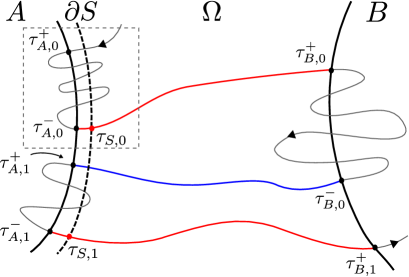
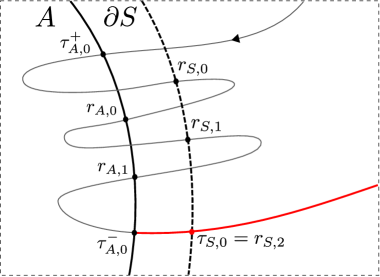
Figure 2. (Left panel) The set $S$ and random times $\tau_{S,j}$. (Right panel) Zoom-in of the boxed region together with stopping times $r_{S,k}$ and $r_{A,k}$.

Although $\tau_{S,j}$ is not a stopping time with respect to $\mathcal{F}_{t}$, the relation

(2.36) $$\{r_{S,k}\mid k\geq 0,\;\;r_{B,k}<r_{A,k}\}=\{\tau_{S,j}\}_{j=0}^{\infty}$$

holds ${\mathbb{P}}$-almost surely.

Now, let

$$Y^{0}_{t}=X_{(t+\tau_{A,0}^{-})\wedge\tau_{B,0}^{+}},\quad\quad t\geq 0,$$

and let $h_{0}=\tau_{S,0}-\tau_{A,0}^{-}$. Since $F$ is bounded and continuous, and since $h_{0}\to 0$ (${\mathbb{P}}$ almost surely) as $\epsilon\to 0$, we have

(2.37) $$\mathbb{E}[F(X_{\cdot\,+\tau_{A,0}^{-}})]=\mathbb{E}[F(Y^{0}_{\cdot})]=\lim_{\epsilon\to 0}\mathbb{E}[F(Y^{0}_{\cdot\,+h_{0}})].$$

We will show that

$$\lim_{\epsilon\to 0}\mathbb{E}[F(Y^{0}_{\cdot\,+h_{0}})]=\mathbb{E}[g(X_{\tau_{A,0}^{-}})]$$

where $g(x)=\widehat{\mathbb{E}}[F(Y_{\cdot})\mid Y_{0}=x]$.

Let $M$ be the unique (random) integer such that

$$\tau_{S,0}=r_{S,M}.$$

Equivalently, $M=\min\{k\geq 0\mid r_{B,k}<r_{A,k}\}$. Since $r_{B,k}>r_{A,k}$ for all $k<M$, we have

(2.38) $$F(Y^{0}_{\cdot\,+h_{0}})=\sum_{k=0}^{M}F(X_{\cdot\,+r_{S,k}})\mathbb{I}_{r_{B,k}<r_{A,k}}=\sum_{k=0}^{\infty}F(X_{\cdot\,+r_{S,k}})\mathbb{I}_{r_{B,k}<r_{A,k}}\mathbb{I}_{k\leq M}.$$

Observe that the event $\{k\leq M\}$ coincides with the event that $r_{B,j}>r_{A,j}$ for all $j<k$, so the event $\{k\leq M\}$ is measurable with respect to $\mathcal{F}_{r_{S,k}}$. Therefore, we have

$$\mathbb{E}[F(Y^{0}_{\cdot\,+h_{0}})] =\sum_{k=0}^{\infty}\mathbb{E}\left[F(X_{\cdot\,+r_{S,k}})\mathbb{I}_{r_{B,k}<r_{A,k}}\mathbb{I}_{k\leq M}\right]$$

$$=\sum_{k=0}^{\infty}\mathbb{E}\left[\;\mathbb{E}[F(X_{\cdot\,+r_{S,k}})\mathbb{I}_{r_{B,k}<r_{A,k}}\mathbb{I}_{k\leq M}\mid\mathcal{F}_{r_{S,k}}]\;\right]$$

$$=\sum_{k=0}^{\infty}\mathbb{E}\left[\mathbb{I}_{k\leq M}\;\mathbb{E}[F(X_{\cdot\,+r_{S,k}})\mathbb{I}_{r_{B,k}<r_{A,k}}\mid\mathcal{F}_{r_{S,k}}]\;\right]$$

$$=\sum_{k=0}^{\infty}\mathbb{E}\left[\mathbb{I}_{k\leq M}\;f(X_{r_{S,k}})\;\right],$$

where

$$f(x)=\mathbb{E}[F(X_{\cdot})\mathbb{I}_{\tau_{B}<\tau_{A}}\mid X_{0}=x]=q(x)\widehat{\mathbb{E}}[F(Y_{\cdot})\mid Y_{0}=x].$$

The last equality follows from the Doob $h$-transform (since $x\in\partial S\subset\Theta$ here). Since $q(x)=\epsilon$ for all $x\in\partial S$, this means

(2.39) $$\mathbb{E}[F(Y^{0}_{\cdot\,+h_{0}})]=\epsilon\,\mathbb{E}\left[\sum_{k=0}^{M}\;g(X_{r_{S,k}})\;\right]$$

where $g(x)=\widehat{\mathbb{E}}[F(Y_{\cdot})\mid Y_{0}=x]$. Note that the random integer $M$ depends on $\epsilon$.

Let $A_{j}$ denote the event $\{j<M\}$, which occurs if and only if $r_{A,k}<r_{B,k}$ for all $k\in\{0,1,\dots,j\}$. Since $q(x)=\epsilon$ for all $x\in\partial S$, the event $A_{j}$ is independent of $X_{r_{S,j}}\in\partial S$. Moreover, $P(A_{j})=(1-\epsilon)^{j+1}$, since

$${\mathbb{P}}(A_{j}) =\mathbb{E}\left[\prod_{k=0}^{j}\mathbb{I}_{r_{A,k}<r_{B,k}}\right]$$

$$=\mathbb{E}\left[\;\prod_{k=0}^{j-1}\mathbb{I}_{r_{A,k}<r_{B,k}}\;\mathbb{E}[\mathbb{I}_{r_{A,j}<r_{B,j}}\mid\mathcal{F}_{r_{S,j}}]\;\right]=(1-\epsilon){\mathbb{P}}(A_{j-1}).$$

Similarly, ${\mathbb{P}}(M=j)=\epsilon(1-\epsilon)^{j}$. Now we evaluate (2.39):

$$\mathbb{E}[F(Y^{0}_{\cdot\,+h_{0}})] =\epsilon\,\mathbb{E}[g(X_{r_{S,0}})]+\epsilon\,\mathbb{E}\left[\sum_{k=1}^{M}\;g(X_{r_{S,k}})\;\right]$$

$$=\epsilon\,\mathbb{E}[g(X_{r_{S,0}})]+\epsilon\,\mathbb{E}\left[\sum_{j=0}^{\infty}\mathbb{I}_{A_{j}}\;g(X_{r_{S,j+1}})]\;\right]$$

$$=\epsilon\,\mathbb{E}[g(X_{r_{S,0}})]+\epsilon\sum_{j=0}^{\infty}\mathbb{E}\left[\mathbb{I}_{A_{j}}\;g(X_{r_{S,j+1}})\;\right]$$

$$=\epsilon\,\mathbb{E}[g(X_{r_{S,0}})]+\epsilon\sum_{j=0}^{\infty}{\mathbb{P}}(A_{j})\,\mathbb{E}\left[\;g(X_{r_{S,j+1}})\;\right]$$

$$=\epsilon\,\mathbb{E}[g(X_{r_{S,0}})]+\epsilon\sum_{j=0}^{\infty}(1-\epsilon)^{j+1}\mathbb{E}\left[\;g(X_{r_{S,j+1}})\;\right]$$

$$=\sum_{j=0}^{\infty}\epsilon(1-\epsilon)^{j}\,\mathbb{E}\left[\;g(X_{r_{S,j}})\;\right]$$

$$=\sum_{j=0}^{\infty}{\mathbb{P}}(M=j)\mathbb{E}\left[\;g(X_{r_{S,j}})\;\right]=\mathbb{E}\left[\;g(X_{\tau_{S,0}})\;\right].$$

Now let $\epsilon\to 0$. Since $g(x)$ is bounded and is continuous up to $\partial A$ by Proposition 2.6, we have (by the dominated convergence theorem)

(2.40) $$\lim_{\epsilon\to 0}\mathbb{E}[g(X_{\tau_{S,0}})]=\mathbb{E}[\lim_{\epsilon\to 0}g(X_{\tau_{S,0}})]=\mathbb{E}[g(X_{\tau_{A,0}^{-}})].$$

∎

3. Reactive Exit and Entrance Distributions

Proof of Lemma 1.3.

The equality (1.19) is equivalent to

$$\int_{\partial\Theta}\rho(x)\widehat{n}(x)\cdot a(x)\nabla q(x)\,\mathrm{d}\sigma_{\Theta}(x)=0.$$

Using (1.16), it is then equivalent to

$$\langle\rho,Lq\rangle=\langle L^{\ast}\rho,q\rangle=0,$$

which is obvious. ∎

Before proving Proposition 1.5, we will need establish some properties of the entrance and exit distributions and of the harmonic measure associated with the generator $L$. These results will also be used later in the paper. First, using integration by parts, we have

Lemma 3.1.

Let $D\subset{\mathbb{R}}^{d}$ be open with smooth boundary. Let $\phi,\psi\in C^{2}(D)\cap C^{1}(\widebar{D})$ and bounded. Then

(3.1) $$\int_{D}\rho(x)\bigl{(}\phi(x)L\psi(x)-\psi(x)\widetilde{L}\phi(x)\bigr{)}\,\mathrm{d}x=\int_{\partial D}\rho(x)b\cdot\widehat{n}(x)\phi(x)\psi(x)\,\mathrm{d}\sigma_{D}(x)\\ +\int_{\partial D}\rho(x)\phi(x)\widehat{n}(x)\cdot a\nabla\psi(x)-\psi(x)\widehat{n}(x)\cdot\operatorname{div}(a(x)\rho(x)\phi(x))\,\mathrm{d}\sigma_{D}(x),$$

where $\widehat{n}(x)$ is the exterior normal vector at $x\in\partial D$.

Let us recall some tools from potential theory (see for example the books [Pinsky:95, Sznitman:98] and also [BoEcGaKl:04, BoGaKl:05] where potential theory was applied to analyze diffusion processes with metastability). The harmonic measure $H_{D}(x,\mathrm{d}y)$ is given by the Poisson kernel corresponding to the boundary value problem

(3.2) $$\begin{cases}Lu(x)=0,&x\in D,\\ u(x)=f(x),&x\in\partial D.\end{cases}$$

Therefore, for $f\in C(\partial D)$,

(3.3) $$u(x)=\int_{\partial D}H_{D}(x,\mathrm{d}y)f(y),$$

is the unique solution to (3.2). Similarly, the harmonic measure $\widetilde{H}_{D}(x,\mathrm{d}y)$ corresponds to the generator $\widetilde{L}$ (recall (1.25)). For the boundary value problem

(3.4) $$\begin{cases}\widetilde{L}\widetilde{u}(x)=0,&x\in D,\\ \widetilde{u}(x)=f(x),&x\in\partial D,\end{cases}$$

the solution is given by

(3.5) $$\widetilde{u}(x)=\int_{\partial D}\widetilde{H}_{D}(x,\mathrm{d}y)f(y).$$

The harmonic measures have a probabilistic interpretation: $H_{D}(x,\mathrm{d}y)$ (resp. $\widetilde{H}_{D}(x,\mathrm{d}y)$) gives the probability that the process associated with the generator $L$ (resp. $\widetilde{L}$) first strikes the boundary $\partial D$ at $\mathrm{d}y$ after starting at $x$. In particular,

$$q(x)=H_{D}(x,\partial B)\quad\text{and}\quad\widetilde{q}(x)=\widetilde{H}_{D}(x,\partial A).$$

We also define the harmonic measures for the conditioned processes as

(3.6) $$H_{\Theta}^{q}(x,\mathrm{d}y)=\frac{q(y)}{q(x)}H_{\Theta}(x,\mathrm{d}y).$$

For $x\in\Theta$ this is a measure on $\partial B$. For $x\in\partial A$ where $q(x)=0$, we may define $H_{\Theta}^{q}(x,\mathrm{d}y)$ through a limit:

(3.7) $$H_{\Theta}^{q}(x,\mathrm{d}y)=\lim_{\begin{subarray}{c}x^{\prime}\in\Theta\\ x^{\prime}\to x\end{subarray}}\frac{q(y)}{q(x)}H_{\Theta}(x,\mathrm{d}y)=\frac{\widehat{n}(x)\cdot a(x)\nabla_{x}H_{\Theta}(x,dy)}{\widehat{n}(x)\cdot a(x)\nabla_{x}q(x)},\quad x\in\partial A.$$

Recall that $q(y)=1$ for $y\in\partial B$.

Recall the reactive exit and entrance measures $\eta_{A}^{-}$, $\eta_{A}^{+}$, $\eta_{B}^{-}$ and $\eta_{B}^{+}$. They are connected by harmonic measures as follows:

Proposition 3.2.

(3.8) $$\int_{\partial A}\eta_{A}^{-}(\mathrm{d}x)H_{\Theta}^{q}(x,\mathrm{d}y)=\eta_{B}^{+}(\mathrm{d}y).$$

(3.9) $$\int_{\partial A}\eta_{A}^{+}(\mathrm{d}x)H_{\widebar{B}^{C}}(x,\mathrm{d}y)=\eta_{B}^{+}(\mathrm{d}y).$$

(3.10) $$\int_{\partial B}\eta_{B}^{+}(\mathrm{d}x)H_{\widebar{A}^{C}}(x,\mathrm{d}y)=\eta_{A}^{+}(\mathrm{d}y).$$

Proof.

We prove (3.8) first. If $f\in C(\partial B)$, let $u_{f}(x)$ solve $Lu=0$ in $\Theta$ with

(3.11) $$u=\begin{cases}f(x),&x\in\partial B,\\ 0,&x\in\partial A.\end{cases}$$

Hence $u(x)\widetilde{q}(x)=0$ on $\partial\Theta$. By applying (3.1) with $\phi(x)=\widetilde{q}(x)$ and $\psi(x)=u_{f}(x)$, we obtain

(3.12) $$\int_{\partial A}\rho(x)\widehat{n}(x)\cdot a(x)\nabla u_{f}(x)\,\mathrm{d}\sigma_{A}(x) =\int_{\partial B}f(x)\widehat{n}(x)\cdot\operatorname{div}(a(x)\rho(x)\widetilde{q}(x))\,\mathrm{d}\sigma_{B}(x)$$

$$=\int_{\partial B}f(x)\rho(x)\widehat{n}(x)\cdot a(x)\nabla\widetilde{q}(x)\,\mathrm{d}\sigma_{B}(x)$$

$$=-\int_{\partial B}f(x)\eta_{B}^{+}(dx).$$

From (3.7) and (1.20), we see that for all $x\in\partial A$,

$$\int_{\partial A}\eta_{A}^{-}(\mathrm{d}x)H_{\Theta}^{q}(x,\mathrm{d}y)=-\int_{\partial A}\rho(x)\widehat{n}(x)\cdot a(x)\nabla_{x}H_{\Theta}(x,\mathrm{d}y)\,\mathrm{d}\sigma_{A}(x).$$

Hence for any $f\in C(\partial B)$, we have

$$\int_{\partial B}\left(\int_{\partial A}\eta_{A}^{-}(\mathrm{d}x)H^{q}_{\Theta}(x,\mathrm{d}y)\right)f(y) =-\int_{\partial B}\int_{\partial A}\rho(x)\widehat{n}(x)\cdot a(x)\nabla_{x}\left(f(y)H_{\Theta}(x,\mathrm{d}y)\right)\,\mathrm{d}\sigma_{A}(x)$$

$$=-\int_{\partial A}\rho(x)\widehat{n}(x)\cdot a(x)\nabla_{x}\left(\int_{\partial B}H_{\Theta}(x,\mathrm{d}y)f(y)\right)\mathrm{d}\sigma_{A}(x)$$

$$=-\int_{\partial A}\rho(x)\widehat{n}(x)\cdot a(x)\nabla_{x}u_{f}(x)\,\mathrm{d}x.$$

Combining this with (3.12), we conclude that

$$\int_{\partial B}\left(\int_{\partial A}\eta_{A}^{-}(\mathrm{d}x)H^{q}_{\Theta}(x,\mathrm{d}y)\right)f(y)=\int_{\partial B}f(x)\eta_{B}^{+}(\mathrm{d}x),\quad\forall\;f\in C(\partial B),$$

which proves (3.8).

To prove (3.9), let $\psi$ solve $L\psi=0$ for $x\in\widebar{B}^{C}$ with $\psi=f$ on $\partial B$. Then by (3.1) with $\phi=1-\widetilde{q}$, we have

$$\int_{\partial A}\eta_{A}^{+}(\mathrm{d}x)\psi(x) =\int_{\partial A}\rho(x)\widehat{n}(x)\cdot a(x)\nabla\widetilde{q}(x)\psi(x)\,\mathrm{d}\sigma_{A}(x)$$

$$=-\int_{\partial A}\rho(x)\widehat{n}(x)\cdot a(x)\nabla(1-\widetilde{q}(x))\psi(x)\,\mathrm{d}\sigma_{A}(x)$$

$$=-\int_{\partial A}\psi(x)\widehat{n}(x)\cdot\operatorname{div}(a\rho(1-\widetilde{q}))\,\mathrm{d}\sigma_{A}(x)\qquad\bigl{(}\text{since }1-\widetilde{q}=0\text{ on }\partial A\bigr{)}$$

$$=\int_{\partial B}f\widehat{n}\cdot\operatorname{div}(a\rho(1-\widetilde{q}))\,\mathrm{d}\sigma_{B}(x)-\int_{\partial B}f\rho b\cdot\widehat{n}\,\mathrm{d}\sigma_{B}(x)$$

$$\qquad\qquad-\int_{\partial B}\rho\widehat{n}\cdot a\nabla\psi\,\mathrm{d}\sigma_{B}(x).$$

Applying (3.1) with the function $\phi\equiv 1$, we also find that

$$0=-\int_{\partial B}f\widehat{n}\cdot\operatorname{div}(a\rho)\,\mathrm{d}\sigma_{B}(x)+\int_{\partial B}f\rho b\cdot\widehat{n}\,\mathrm{d}\sigma_{B}(x)+\int_{\partial B}\rho\widehat{n}\cdot a\nabla\psi\,\mathrm{d}\sigma_{B}(x).$$

Therefore, since $1-\widetilde{q}=1$ on $\partial B$, we conclude that

$$\int_{\partial A}\eta_{A}^{+}(\mathrm{d}x)\psi(x) =\int_{\partial B}f\widehat{n}\cdot\operatorname{div}(a\rho(1-\widetilde{q}))\,\mathrm{d}\sigma_{B}(x)-\int_{\partial B}f\widehat{n}(x)\cdot\operatorname{div}(a\rho)\,\mathrm{d}\sigma_{B}(x)$$

$$=\int_{\partial B}f\rho\widehat{n}\cdot a\nabla(1-\widetilde{q})\,\mathrm{d}\sigma_{B}(x)$$

$$=-\int_{\partial B}f\rho\widehat{n}\cdot a\nabla\widetilde{q}\,\mathrm{d}\sigma_{B}(x)=\int_{\partial A}f\eta_{B}^{+}(\mathrm{d}x).$$

We arrive at (3.9) noting that

$$\psi(x)=\int_{\partial B}H_{\widebar{B}^{C}}(x,\mathrm{d}y)f(y).$$

We omit the proof of (3.10) which is analogous to that of (3.9) by switching the role of $A$ and $B$. ∎

By combining (3.9) and (3.10) we immediately obtain the following:

Corollary 3.3.

Let $P_{B}(x,\mathrm{d}y)$ be the probability transition kernel

$$P_{B}(x,\mathrm{d}y)=\int_{\partial A}H_{\widebar{A}^{C}}(x,\mathrm{d}z)H_{\widebar{B}^{C}}(z,\mathrm{d}y),\quad x,y\in\partial B$$

on $\partial B$, and let $P_{A}(x,\mathrm{d}y)$ be the probability transition kernel

$$P_{A}(x,\mathrm{d}y)=\int_{\partial B}H_{\widebar{B}^{C}}(x,\mathrm{d}z)H_{\widebar{A}^{C}}(z,\mathrm{d}y),\quad x,y\in\partial A$$

on $\partial A$. Then

$$\int_{x\in\partial B}\eta_{B}^{+}(\mathrm{d}x)P_{B}(x,\mathrm{d}y)=\eta_{B}^{+}(\mathrm{d}y).$$

and

$$\int_{x\in\partial A}\eta_{A}^{+}(\mathrm{d}x)P_{A}(x,\mathrm{d}y)=\eta_{A}^{-}(\mathrm{d}y).$$

That is, $\eta_{B}^{+}$ and $\eta_{A}^{+}$ are invariant under $P_{B}$ and $P_{A}$, respectively.

We are ready to return to the proof of Proposition 1.5.

Proof of Proposition 1.5.

We first verify that $\eta_{B}^{+}$ is a probability measure. Taking $\psi=q$ and $\phi=\widetilde{q}$ in (3.1), we obtain using the boundary conditions of $q$ and $\widetilde{q}$ on $\partial A$ and $\partial B$,

$$\eta_{A}^{-}(\partial A)=\frac{1}{\nu}\int_{\partial_{A}}\rho\widehat{n}\cdot a\nabla q\,\mathrm{d}\sigma_{A} =\frac{1}{\nu}\int_{\partial B}\widehat{n}\cdot\operatorname{div}(a\rho\widetilde{q})\,\mathrm{d}\sigma_{B}$$

$$=\frac{1}{\nu}\int_{\partial B}\widehat{n}\cdot a\rho\nabla\widetilde{q}\,\mathrm{d}\sigma_{B}=\eta_{B}^{+}(\partial B).$$

This shows that $\eta_{B}^{+}(\partial B)=1$ and $\nu$ is the correct normalization constant.

Let $g$ be a positive continuous function on $\partial B$. Define for $x\not\in\widebar{B}$,

(3.13) $$u(x)={\mathbb{E}}\left[g(X_{\tau_{B}})\mid X_{0}=x\right].$$

Hence $u$ satisfies the equation

(3.14) $$\begin{cases}Lu(x)=0,&x\in\widebar{B}^{c};\\ u(x)=g(x),&x\in\partial B.\end{cases}$$

Let $H_{\widebar{B}^{c}}(x,\mathrm{d}y)$ be the harmonic measure (the measure of the first hitting point on $\widebar{B}$ for the process starting at $x$). We have

(3.15) $$u(x)=\int_{\partial B}H_{\widebar{B}^{c}}(x,\mathrm{d}y)g(y).$$

By the maximum principle, $u>0$ in $\widebar{B}^{C}$. By the Harnack inequality and the compactness of $\partial A$, we have

(3.16) $$\sup_{x\in\partial A}u(x)\leq C\inf_{x\in\partial A}u(x)$$

where the constant $C>0$ only depends on the elliptic constants of $a$; in particular, $C$ is independent of $g$. Therefore, we obtain for any $x,x^{\prime}\in\partial A$, $y\in\partial B$

(3.17) $$0<C^{-1}\leq\frac{H_{\widebar{B}^{c}}(x,\mathrm{d}y)}{H_{\widebar{B}^{c}}(x^{\prime},\mathrm{d}y)}\leq C<\infty.$$

If we define

(3.18) $$\nu(\mathrm{d}y)=\inf_{x\in\partial A}H_{\widebar{B}^{c}}(x,\mathrm{d}y),$$

then $\nu(\mathrm{d}y)>0$ on $\partial B$ and

(3.19) $$H_{\widebar{B}^{c}}(x,\mathrm{d}y)\geq C^{-1}\nu(\mathrm{d}y)$$

for any $x\in\partial A$.

Consider the Markov chain given by $\{X_{\tau_{B,k}^{+}}\}_{k=0}^{\infty}$ on $\partial B$. Let $P_{B}$ denote its transition kernel, given by

(3.20) $$P_{B}(y,\mathrm{d}y^{\prime})=\int_{\partial A}H_{\widebar{A}^{c}}(y,\mathrm{d}x)H_{\widebar{B}^{c}}(x,\mathrm{d}y^{\prime}).$$

By (3.19), $P_{B}$ satisfies Doeblin’s condition:

(3.21) $$P_{B}(y,\mathrm{d}y^{\prime})\geq C^{-1}\int_{\partial A}H_{\widebar{A}^{c}}(y,\mathrm{d}x)\nu(\mathrm{d}y)=C^{-1}\nu(\mathrm{d}y).$$

Therefore, $P_{B}$ has a unique invariant measure. By Corollary 3.3, this invariant measure is given by $\eta_{B}^{+}$. The convergence in Proposition 1.5 now follows (see e.g. [MeTw:09]). ∎

Proof of Theorem 1.7.

Consider the family of processes

$$X^{A,n}_{t}=X_{(t+\tau_{A,n}^{+})\wedge\tau_{B,n}^{+}}.$$

Observe that the $n^{th}$ reactive trajectory $t\mapsto Y^{n}_{t}$ is a subset of the path $t\mapsto X^{A,n}_{t}$; specifically, $Y^{n}_{t}=X^{A,n}_{t+\tau_{A,n}^{-}-\tau_{A,n}^{+}}$ for all $t\geq 0$. The random sequence of points

$$y_{n}=X^{A,n}_{0}=X_{\tau_{A,n}^{+}}\in\partial A,\quad n=0,1,2,\dots$$

corresponds to a Markov chain on the state space $\partial A$ with transition kernel

$$P_{A}(x,\mathrm{d}y)={\mathbb{P}}(y_{n+1}\in\mathrm{d}y\mid y_{n}=x)=\int_{\partial B}H_{\widebar{B}^{C}}(x,\mathrm{d}z)H_{\widebar{A}^{C}}(z,\mathrm{d}y).$$

As shown in the proof of Proposition 1.5, this chain has a unique invariant probability distribution $\eta_{A}^{+}$ supported on $\partial A$:

$$\int_{\partial A}\eta_{A}^{+}(\mathrm{d}x)P_{A}(x,\mathrm{d}y)=\eta_{A}^{+}(\mathrm{d}y).$$

The sequence of processes $t\mapsto X^{A,n}_{t}$ corresponds to a Markov chain on the metric space $\mathcal{X}=C([0,\infty))$. It can be shown that this is a Harris chain with unique invariant distribution

$$\widebar{\mathcal{P}}(U)=\int_{\partial A}\eta_{A}^{+}(\mathrm{d}x)\mathcal{P}_{x}(U),\quad\forall\;U\in\mathcal{B}$$

where $\mathcal{P}_{x}$ denotes the law on $(\mathcal{X},\mathcal{B})$ of the process $t\mapsto Z_{t\wedge\tau_{B}}$ where

$$\,\mathrm{d}Z_{t}=b(Z_{t})\,\mathrm{d}t+\sqrt{2}\,\sigma(Z_{t})\,\mathrm{d}W_{t},\quad Z_{0}=x$$

and $\tau_{B}$ is the first hitting time of $Z_{t}$ to $\widebar{B}$. (The uniqueness of $\widebar{\mathcal{P}}$ follows from the uniqueness of $\eta_{A}^{+}$ as an invariant distribution for the chain defined by transition kernel $P_{A}$ on $\partial A$.) Therefore (see e.g. [MeTw:09]), for any $\Phi\in L^{1}(\mathcal{X},\mathcal{B},\widebar{\mathcal{P}})$ the limit

(3.22) $$\lim_{N\to\infty}\frac{1}{N}\sum_{k=1}^{N}\Phi(X^{A,k})=\mathbb{E}[\Phi(Z_{\cdot\wedge\tau_{B}})\mid Z_{0}\sim\eta_{A}^{+}]$$

holds ${\mathbb{P}}$-almost surely.

Using (3.22) we will establish the following relationship between $\eta_{A}^{-}$ and $\eta_{A}^{+}$:

Lemma 3.4.

Let $X_{t}$ satisfy the SDE (1.1) with initial distribution $X_{0}\sim\eta_{A}^{+}$ on $\partial A$. Then for any Borel set $U\subset\partial A$,

$${\mathbb{P}}(X_{\tau_{A,0}^{-}}\in U\mid X_{0}\sim\eta_{A}^{+})=\eta_{A}^{-}(U)=-\frac{1}{\nu}\int_{U}\rho(x)\widehat{n}(x)\cdot a(x)\nabla q(x)\,\mathrm{d}\sigma_{A}(x).$$

Proof of Lemma 3.4..

Let $f\in C({\mathbb{R}}^{d})$ be bounded and non-negative. Then by applying (3.22) to the functional $\Phi(X)=f(X_{\tau_{S,0}^{-}})$, we obtain

$$\lim_{\epsilon\to 0}\lim_{N\to\infty}\frac{1}{N}\sum_{n=0}^{N-1}f(X_{\tau_{S,n}}) =\lim_{\epsilon\to 0}\mathbb{E}[f(X_{\tau_{S,0}})\mid X_{0}\sim\eta_{A}^{+}]$$

$$=\mathbb{E}[f(X_{\tau_{A,0}^{-}})\mid X_{0}\sim\eta_{A}^{+}].$$

We also have,

(3.23) $$\lim_{N\to\infty}\frac{1}{N}\sum_{n=0}^{N-1}f(X_{\tau_{S,n}}) =\lim_{K\to\infty}\frac{K}{N_{K}}\lim_{K\to\infty}\frac{1}{K}\sum_{k=0}^{K-1}f(X_{r_{S,k}})\mathbb{I}_{r_{B,k}<r_{A,k}}=\int_{\partial S}f(x)\zeta_{S}(\mathrm{d}x),$$

holds ${\mathbb{P}}$-almost surely, where $N_{K}=|\{k\in\{0,1,\dots,K-1\}\mid r_{B,k}<r_{A,k}\}|$. Here we have used $\zeta_{S}$ to denote the unique invariant distribution (identified below) for the Markov chain defined by $X_{r_{S,k}}$ on $\partial S$. Therefore,

$$\mathbb{E}\,[f(X_{\tau_{A,0}^{-}})\mid X_{0}\sim\eta_{A}^{+}]=\lim_{\epsilon\to 0}\int_{\partial S}f(x)\zeta_{S}(\mathrm{d}x).$$

We claim that if $f(x)$ is uniformly continuous in a neighborhood of $\partial A$, then

(3.24) $$\lim_{\epsilon\to 0}\int_{\partial S}\zeta_{S}(\mathrm{d}x)f(x)=\int_{\partial A}\eta_{A}^{-}(\mathrm{d}x)f(x).$$

First, let us identify the invariant distribution $\zeta_{S}$. By applying Corollary 3.3 (replacing $B$ by $\widebar{S}^{C}$) we can identify $\zeta_{S}$ as

$$\zeta_{S}(\mathrm{d}x)\;(=\eta_{S}^{+}(\mathrm{d}x))=-\frac{\epsilon}{\nu}\rho(x)\widehat{n}(x)\cdot a(x)\nabla\widetilde{q}_{S}(x)\,\mathrm{d}\sigma_{S}(x),$$

where $\widehat{n}(x)$ is the exterior normal at $x\in\partial S$, and $\widetilde{q}_{S}$ satisfies $\widetilde{L}\widetilde{q}_{S}=0$ in $S$ with

$$\widetilde{q}_{S}(x)=\begin{cases}1,&x\in\partial A\\ 0,&x\in\partial S.\end{cases}$$

Note that $\nu$ is independent of $\epsilon$. Let $\delta>\epsilon$ be small, and suppose that $f(x)$ is continuous on the closed set $\{x\in\widebar{\Theta}\mid 0\leq q(x)\leq\delta\}$. (This set contains both $\partial A$ and $\partial S$). A computation similar to (3.12) (replacing $B$ by $S$) shows that for any such function, we have

(3.25) $$\int_{\partial S}\zeta_{S}(\mathrm{d}x)f(x)=-\frac{\epsilon}{\nu}\int_{\partial A}\rho(x)\widehat{n}(x)\cdot a(x)\nabla u_{f,S}(x)\,\mathrm{d}\sigma_{A}(x),$$

where $u_{f,S}$ satisfies $Lu=0$ in $S\setminus\widebar{A}$, and

$$u_{f,S}(x)=\begin{cases}f(x),&x\in\partial S\\ 0,&x\in\partial A.\end{cases}$$

Since $f\geq 0$, we have $u>0$ in $S\setminus\widebar{A}$. Now, let us define

$$z_{f,S}(x)=\epsilon\frac{u_{f,S}(x)}{q(x)},\quad x\in\widebar{S}\setminus A,$$

which satisfies $L^{q}z=0$ in $S\setminus\widebar{A}$, with $z=f$ on $\partial S$ (recall that $q(x)=\epsilon$ for all $x\in\partial S$). By the boundary Harnack inequality ([Bau:84, CS:05]), $z_{f,S}(x)$ is bounded and Hölder continuous on $\widebar{S}\setminus A$ (including $\partial A$). We claim that for any $x_{0}\in\partial A$, we have

(3.26) $$\lim_{x\to x_{0}}\nabla u_{f,S}(x)=\epsilon^{-1}z_{f,S}(x_{0})\nabla q(x_{0}).$$

Since $\nabla u_{f,S}$, $\nabla q$, and $z_{f,S}$ are continuous up to $\partial A$, this is true if and only if

$$\lim_{x\to x_{0}}q(x)\nabla z_{f,S}(x)=0.$$

Suppose $q(x)\nabla z_{f,S}(x)\to v\neq 0$ as $x\to x_{0}\in\partial A$. Then we must have

$$\lim_{x\to x_{0}}\nabla u_{f,S}(x)-z_{f,S}(x)\nabla q(x)=v$$

so that $v$ must be a multiple of $\widehat{n}(x_{0})$ (since $u$ and $q$ vanish on $\partial A$). Thus, we would have

(3.27) $$\widehat{n}(x_{0})\cdot\nabla z_{f,S}(x)\sim(\widehat{n}(x_{0})\cdot v)q(x)^{-1}$$

as $x\to x_{0}\in\partial A$. If $v\neq 0$, then $(\widehat{n}(x_{0})\cdot v)\neq 0$, so (3.27) and the fact that $q=0$ on $\partial A$ would contradict the boundedness of $z_{f,S}(x)$. Therefore, (3.26) must hold.

Combining (3.25) and (3.26) we obtain

$$\int_{\partial S}\zeta_{S}(\mathrm{d}x)f(x)=-\frac{1}{\nu}\int_{\partial A}\rho(x)\widehat{n}(x)\cdot a(x)\nabla q(x)z_{f,S}(x)\,\mathrm{d}\sigma_{A}(x)=\int_{\partial A}\eta_{A}^{-}(\mathrm{d}x)z_{f,S}(x).$$

Therefore, as $\epsilon\to 0$,

(3.28) $$\lim_{\epsilon\to 0}\int_{\partial S}\zeta_{S}(\mathrm{d}x)f(x)=\lim_{\epsilon\to 0}\int_{\partial A}\eta_{A}^{-}(\mathrm{d}x)z_{f,S}(x)=\int_{\partial A}\eta_{A}^{-}(\mathrm{d}x)f(x).$$

This establishes (3.24) and completes the proof of Lemma 3.4. ∎

Now we continue with the proof of Theorem 1.7. We will apply Theorem 1.2. Suppose that $F\in L^{1}(\mathcal{X},\mathcal{B},\mathcal{Q}_{\eta_{A}^{-}})$, and define the functional

$$\Phi(X)=F(X_{(\cdot+\tau_{A,0}^{-})\wedge\tau_{B,0}^{+}}).$$

Combining Theorem 1.2 and Lemma 3.4 we see that $\Phi\in L^{1}(\mathcal{X},\mathcal{B},\widebar{\mathcal{P}})$, since

$$\widebar{\mathcal{P}}(\Phi(X)>\alpha) ={\mathbb{P}}(\Phi(X)>\alpha\mid X_{0}\sim\eta_{A}^{+})$$

$$={\mathbb{P}}(F(X_{(\cdot\,+\tau_{A,0}^{-})\wedge\tau_{B_{0}}^{+}})>\alpha\mid X_{0}\sim\eta_{A}^{+})$$

$$=\mathbb{Q}(F(Y)>\alpha\mid Y_{0}\sim\eta_{A}^{-})=\mathcal{Q}(F(Y)>\alpha).$$

Therefore,

$$\frac{1}{N}\sum_{k=0}^{N-1}F(Y^{k})=\frac{1}{N}\sum_{k=0}^{N-1}F(X^{A,k}_{(\cdot+\tau_{A,k}^{-})\wedge\tau_{B,k}^{+}})=\frac{1}{N}\sum_{k=0}^{N-1}\Phi(X^{A,k}_{\cdot}).$$

By (3.22) and Theorem 1.2, we now conclude that the limit

$$\lim_{N\to\infty}\frac{1}{N}\sum_{k=0}^{N-1}F(Y^{k})=\mathbb{E}[\Phi(Z_{\cdot\wedge\tau_{B}})\mid Z_{0}\sim\eta_{A}^{+}]=\widehat{\mathbb{E}}[F(Y)\mid Y_{0}\sim\eta_{A}^{-}]$$

holds ${\mathbb{P}}$-almost surely. This completes the proof of Theorem 1.7. ∎

4. Reaction rate, density and current of transition paths

4.1. Reaction rate

Proof of Proposition 1.8.

Denote $\tau_{B}$ the first hitting time of $X_{t}$ to $\widebar{B}$. Consider the mean first hitting time

$$u_{B}(x)=\mathbb{E}\left[\tau_{B}\mid X_{0}=x\right],$$

which satisfies the equation

(4.1) $$\begin{cases}Lu_{B}(x)=-1,&x\in\Theta\\ u_{B}(x)=0,&x\in\partial B.\end{cases}$$

By definition of $\eta_{A}^{+}$, we have

(4.2) $$\int_{\partial A}\eta_{A}^{+}(\mathrm{d}x)u_{B}(x) =\frac{1}{\nu}\int_{\partial A}\rho(x)u_{B}(x)\widehat{n}(x)\cdot a(x)\nabla\widetilde{q}(x)\,\mathrm{d}\sigma_{A}(x).$$

Observe that

$$\int_{\mathbb{R}^{d}}\rho(x)\widetilde{q}(x)\,\mathrm{d}x =\int_{B^{c}}\rho(x)\widetilde{q}(x)\,\mathrm{d}x$$

$$\stackrel{{\scriptstyle\eqref{eq:defuB}}}{{=}}-\int_{B^{c}}\rho(x)\widetilde{q}(x)(Lu_{B})(x)\,\mathrm{d}x$$

$$=-\int_{A}\rho(x)(Lu_{B})(x)\,\mathrm{d}x-\int_{\Theta}\rho(x)\widetilde{q}(x)(Lu_{B})(x)\,\mathrm{d}x.$$

Using (3.1) with $D=A$, $\phi(x)=1$ and $\psi(x)=u_{B}$, we obtain

$$\int_{A}\rho(Lu_{B})\,\mathrm{d}x=-\int_{\partial A}\rho b\cdot\widehat{n}u_{B}\,\mathrm{d}\sigma_{A}(x)-\int_{\partial A}\rho\widehat{n}\cdot a\nabla u_{B}\,\mathrm{d}\sigma_{A}(x)+\int_{\partial A}u_{B}\widehat{n}\cdot\operatorname{div}(a\rho)\,\mathrm{d}\sigma_{A}(x),$$

where $\widehat{n}$ is the interior normal vector at $\partial A$. Apply (3.1) again with $D=\Theta$, $\phi=\widetilde{q}$ and $\psi=u_{B}$,

$$\int_{\Theta}\rho\widetilde{q}(Lu_{B})\,\mathrm{d}x=\int_{\partial A}\rho b\cdot\widehat{n}u_{B}\,\mathrm{d}\sigma_{A}(x)+\int_{\partial A}\rho\widehat{n}\cdot a\nabla u_{B}\,\mathrm{d}\sigma_{A}(x)-\int_{\partial A}u_{B}\widehat{n}\cdot\operatorname{div}(a\rho\widetilde{q})\,\mathrm{d}\sigma_{A}(x).$$

Combining the two with (4.2), we get

$$\int_{\partial A}\eta_{A}^{+}(\mathrm{d}x)u_{B}(x)=\frac{1}{\nu}\int_{\partial A}\rho u_{B}\widehat{n}\cdot a\nabla\widetilde{q}\,\mathrm{d}\sigma_{A}(x)=\frac{1}{\nu}\int_{\mathbb{R}^{d}}\rho\widetilde{q}\,\mathrm{d}x.$$

Similarly, defining $u_{A}(x)$ to be the mean first hitting time of $X_{t}$ to $\widebar{A}$ starting at $x$, we have

$$\int_{\partial B}\eta_{B}^{+}(\mathrm{d}x)u_{A}(x)=\frac{1}{\nu}\int_{\mathbb{R}^{d}}\rho(1-\widetilde{q})\,\mathrm{d}x.$$

Add the integrals together to obtain

$$\int_{\partial A}\eta_{A}^{+}(\mathrm{d}x)u_{B}(x)+\int_{\partial B}\eta_{B}^{+}(\mathrm{d}x)u_{A}(x)=\frac{1}{\nu}.$$

On the other hand, observe that

$$\frac{1}{\nu_{R}} =\lim_{N_{T}\to\infty}\frac{T}{N_{T}}$$

$$=\lim_{N\to\infty}\frac{1}{N}\sum_{n=0}^{N-1}(\tau_{A,n+1}^{+}-\tau_{A,n}^{+})$$

$$=\lim_{N\to\infty}\frac{1}{N}\sum_{n=0}^{N-1}(\tau_{B,n}^{+}-\tau_{A,n}^{+})+\lim_{N\to\infty}\frac{1}{N}\sum_{n=0}^{N-1}(\tau_{A,n+1}^{+}-\tau_{B,n}^{+}).$$

As $N\to\infty$, we have

$$T_{AB}=\lim_{N\to\infty}\frac{1}{N}\sum_{n=0}^{N-1}(\tau_{B,n}^{+}-\tau_{A,n}^{+})=\mathbb{E}[\tau_{B}\mid X_{0}\sim\eta_{A}^{+}]=\int_{\partial A}\eta_{A}^{+}(\mathrm{d}x)u_{B}(x),$$

and similarly

$$T_{BA}=\lim_{N\to\infty}\frac{1}{N}\sum_{n=0}^{N-1}(\tau_{A,n+1}^{+}-\tau_{B,n}^{+})=\int_{\partial B}\eta_{B}^{+}(\mathrm{d}x)u_{A}(x).$$

Therefore

$$\frac{1}{\nu_{R}}=\int_{\partial A}\eta_{A}^{+}(\mathrm{d}x)u_{B}(x)+\int_{\partial B}\eta_{B}^{+}(\mathrm{d}x)u_{A}(x)=\frac{1}{\nu},$$

or equivalently $\nu=\nu_{R}$.

From Theorem 1.7 it follows immediately that

$$C_{AB}=\int_{\partial A}\eta_{A}^{-}(\mathrm{d}x)v_{B}(x).$$

Indeed, the functional $F:Y\to\tau^{Y}_{B}$ is in $L^{1}(\mathcal{X},\mathcal{B},\mathcal{Q}_{\eta_{A}^{-}})$ by Proposition 2.7. The function $v_{B}(x)=\widehat{\mathbb{E}}[\tau_{B}^{Y}\mid Y_{0}=x]$ satisfies

$$L^{q}v_{B}=-1,\quad x\in\Theta$$

with $v(x)=0$ for $x\in\partial B$. Hence, the function $w(x)=q(x)v_{B}(x)$ satisfies $Lw=-q$ for $x\in\Theta$ with boundary condition $w(x)=0$ for $x\in\partial\Theta$. Moreover, for $x_{0}\in\partial A$, we have

$$v_{B}(x_{0})=\lim_{x\to x_{0}}\frac{w(x)}{q(x)}=\frac{\widehat{n}(x_{0})\cdot a(x_{0})\nabla w(x_{0})}{\widehat{n}(x_{0})\cdot a(x_{0})\nabla q(x_{0})}.$$

Therefore,

$$\int_{\partial A}\eta_{A}^{-}(\mathrm{d}x)v_{B}(x)=-\frac{1}{\nu}\int_{\partial A}\rho(x)\widehat{n}(x)\cdot a(x)\nabla w(x)\,\mathrm{d}\sigma_{A}(x).$$

Now applying (3.1) with $D=\Theta$, $\phi=\tilde{q}$ and $\psi=w$, we have

$$-\frac{1}{\nu}\int_{\partial A}\rho(x)\widehat{n}(x)\cdot a(x)\nabla w(x)\,\mathrm{d}\sigma_{A}(x)=\frac{1}{\nu}\int_{\Theta}\rho(x)\tilde{q}(x)q(x)\,\mathrm{d}x.$$

It remains to show that

$$\nu=\int_{\mathbb{R}^{d}}\rho\nabla q\cdot a\nabla q\,\mathrm{d}x.$$

Using integration by parts, we have

$$\int_{\mathbb{R}^{d}}\rho\nabla q\cdot a\nabla q\,\mathrm{d}x =\int_{\Theta}\rho\nabla\bigl{(}q-\frac{1}{2}\bigr{)}\cdot a\nabla q\,\mathrm{d}x$$

$$=-\int_{\Theta}\nabla\cdot(\rho a\nabla q)\bigl{(}q-\frac{1}{2}\bigr{)}\,\mathrm{d}x+\int_{\partial A}\rho\bigl{(}q-\frac{1}{2}\bigr{)}\widehat{n}\cdot a\nabla q\,\mathrm{d}\sigma_{A}(x)$$

$$\hskip 130.0002pt+\int_{\partial B}\rho\bigl{(}q-\frac{1}{2}\bigr{)}\widehat{n}\cdot a\nabla q\,\mathrm{d}\sigma_{B}(x).$$

The first term on the right hand side vanishes as

$$\int_{\Theta}\nabla\cdot(\rho a\nabla q)\bigl{(}q-\frac{1}{2}\bigr{)}\,\mathrm{d}x =\int_{\Theta}\Bigl{(}\rho\operatorname{tr}a\nabla^{2}q+\rho b\cdot\nabla q\Bigr{)}\bigl{(}q-\frac{1}{2}\bigr{)}\,\mathrm{d}x$$

$$\quad+\frac{1}{2}\int_{\Theta}\Bigl{(}\operatorname{div}(\rho a)\cdot\nabla-\rho b\nabla\Bigr{)}(q^{2}-q)\,\mathrm{d}x$$

$$=\int_{\Theta}\rho(Lq)\bigl{(}q-\frac{1}{2}\bigr{)}\,\mathrm{d}x-\frac{1}{2}\int_{\Theta}(L^{\ast}\rho)(q^{2}-q)=0,$$

where we have used that $q^{2}-q=0$ on $\partial A\cup\partial B$. The conclusion then follows from Lemma 1.3, $q=0$ on $\partial A$, and $q=1$ on $\partial B$. ∎

4.2. Density of transition paths

We define the Green’s function $G_{\Theta}$ of the operator $L$ in $\Theta$ with Dirichlet boundary condition on $\partial\Theta$:

(4.3) $$\begin{cases}LG_{\Theta}(x,y)=-\delta_{y}(x),&x\in\Theta,\\ G_{\Theta}(x,y)=0,&x\in\partial\Theta.\end{cases}$$

The existence of the Green’s function is guaranteed by the ergodicity of $X_{t}$ in ${\mathbb{R}}^{d}$, which implies that $X_{t}$ is transient in $\Theta$ (see e.g. [Pinsky:95]*Section 4.2).

Lemma 4.1.

Let $G_{\Theta}$ be the Green’s function of $L$ in $\Theta$ with Dirichlet boundary condition on $\partial\Theta$. We have

(4.4) $$G_{\Theta}^{q}(x,y)\equiv\int_{0}^{\infty}Q_{R}(t,x,y)\,\mathrm{d}t=\frac{q(y)G_{\Theta}(x,y)}{q(x)}.$$

In particular, for $x\in\partial A$, $y\in\Theta$

(4.5) $$G_{\Theta}^{q}(x,y)=\frac{q(y)\widehat{n}(x)\cdot a(x)\nabla_{x}G_{\Theta}(x,y)}{\widehat{n}(x)\cdot a(x)\nabla q(x)}.$$

Proof.

Fix $y\in\Theta$. For $x\in\Theta$, (4.4) follows from [Pinsky:95]*Proposition 4.2.2. Specifically, the function $G_{\Theta}^{q}(x,y)$ defined by

$$G_{\Theta}^{q}(x,y)=\int_{0}^{\infty}Q_{R}(t,x,y)\,\mathrm{d}t$$

is related to the Green’s function (4.3) by the formula

$$G_{\Theta}^{q}(x,y)=\frac{q(y)G_{\Theta}(x,y)}{q(x)},\quad x,y\in\Theta.$$

Because of the regularity of the coefficients $a(x)$ and $b(x)$, Schauder-type interior and boundary estimates imply that $G(\cdot,y)\in C^{2,\alpha}(\widebar{\Theta}\setminus\{y\})$. Since $G(x,y)=q(x)=0$ for $x\in\partial A$, the Hopf Lemma implies that for all $x\in\partial A$, $\nabla_{x}G(x,y)$ is a nonzero multiple of $\widehat{n}(x)$. That is, for all $x\in\partial A$, $\nabla_{x}G(x,y)=r(x)\widehat{n}(x)$ for some continuous $r(x)<0$. The same is true for $q$. Therefore, $G_{\Theta}^{q}(x,y)$ is continuous in $x$ up to the boundary $\partial\Theta$ and for $x_{0}\in\partial A$,

$$\lim_{x\to x_{0},\,x\in\Theta}G_{\Theta}^{q}(x,y)=\frac{q(y)\widehat{n}(x_{0})\cdot a(x_{0})\nabla_{x}G_{\Theta}(x_{0},y)}{\widehat{n}(x_{0})\cdot a(x_{0})\nabla q(x_{0})}.$$

It remains to show that for $x_{0}\in\partial A$,

(4.6) $$\frac{q(y)\widehat{n}(x_{0})\cdot a(x_{0})\nabla_{x}G_{\Theta}(x_{0},y)}{\widehat{n}(x_{0})\cdot a(x_{0})\nabla q(x_{0})}=\int_{0}^{\infty}Q_{R}(t,x_{0},y)\,\mathrm{d}t.$$

Let $\varphi\geq 0$ be smooth and compactly supported in $\Theta$. By Proposition 2.6, we have

$$\lim_{x\to x_{0}}\widehat{\mathbb{E}}[\varphi(Y_{t})\mid Y_{0}=x]=\widehat{\mathbb{E}}[\varphi(Y_{t})\mid Y_{0}=x_{0}].$$

Moreover,

$$\widehat{\mathbb{E}}[\varphi(Y_{t})\mid Y_{0}=x]\leq\lVert\varphi\rVert_{\infty}\mathbb{Q}(Y_{t}\in\Theta\mid Y_{0}=x).$$

By Proposition 2.7, for any $R>0$, there are constants $k_{1},k_{2}>0$ such that $\mathbb{Q}(Y_{t}\in\Theta\mid Y_{0}=x)\leq k_{1}e^{-k_{2}t}$ for all $x\in\theta$, $|x|<R$, $t\geq 0$. Therefore, we have $\widehat{\mathbb{E}}[\varphi(Y_{t})\mid Y_{0}=x]\leq\lVert\varphi\rVert_{\infty}k_{1}e^{-k_{2}t}$ so the dominated convergence theorem implies that

(4.7) $$\lim_{x\to x_{0}}\int_{\Theta}G_{\Theta}^{q}(x,y)\varphi(y)\,\mathrm{d}y =\lim_{x\to x_{0}}\int_{0}^{\infty}\widehat{\mathbb{E}}[\varphi(Y_{t})\mid Y_{0}=x]\,\mathrm{d}t$$

$$=\int_{0}^{\infty}\widehat{\mathbb{E}}[\varphi(Y_{t})\mid Y_{0}=x_{0}]\,\mathrm{d}t$$

$$=\int_{0}^{\infty}\left(\int_{\Theta}Q(t,x_{0},y)\varphi(y)\,\mathrm{d}y\right)\,\mathrm{d}t.$$

On the other hand, we also have

(4.8) $$\lim_{x\to x_{0}}\int_{\Theta}G_{\Theta}^{q}(x,y)\varphi(y)\,\mathrm{d}y=\int_{\Theta}\frac{q(y)\widehat{n}(x_{0})\cdot a(x_{0})\nabla_{x}G_{\Theta}(x_{0},y)}{\widehat{n}(x_{0})\cdot a(x_{0})\nabla q(x_{0})}\varphi(y)\,\mathrm{d}y.$$

Therefore, by combining (4.7) and (4.8) we conclude

$$\int_{\Theta}\frac{q(y)\widehat{n}(x_{0})\cdot a(x_{0})\nabla_{x}G_{\Theta}(x_{0},y)}{\widehat{n}(x_{0})\cdot a(x_{0})\nabla q(x_{0})}\varphi(y)\,\mathrm{d}y =\int_{0}^{\infty}\int_{\Theta}Q(t,x_{0},y)\varphi(y)\,\mathrm{d}y\,\mathrm{d}t$$

$$=\int_{\Theta}\left(\int_{0}^{\infty}Q(t,x_{0},y)\,\mathrm{d}t\right)\varphi(y)\,\mathrm{d}y.$$

Since $\varphi$ is arbitrary, this implies (4.6). ∎

Proof of Proposition 1.9.

Using Lemma 4.1 and (1.35),

(4.9) $$\rho_{R}(z)=\nu_{R}\int_{\partial A}\eta_{A}^{-}(\mathrm{d}x)G^{q}_{\Theta}(x,z).$$

Recall the explicit formula of $\eta_{A}^{-}$ in terms of $q$ (1.20), we obtain for $z\in\Theta$

$$\rho_{R}(z) =-\int_{\partial A}\rho(x)\frac{q(y)\widehat{n}(x)\cdot a\nabla_{x}G_{\Theta}(x,z)}{\widehat{n}(x)\cdot a\nabla q(x)}\widehat{n}(x)\cdot a\nabla q(x)\,\mathrm{d}\sigma_{A}(x)$$

$$=-q(y)\int_{\partial A}\rho(x)\widehat{n}(x)\cdot a\nabla_{x}G_{\Theta}(x,z)\,\mathrm{d}\sigma_{A}(x).$$

Apply (3.1) by taking $\psi(x)=G_{\Theta}(x,y)$ and $\phi(x)=\widetilde{q}(x)$, we conclude that

$$\rho_{R}(y) =-q(y)\int_{\partial\Theta}\rho(x)\phi(x)\widehat{n}(x)\cdot a\nabla\psi(x)\,\mathrm{d}\sigma_{\Theta}(x)$$

$$=-q(y)\int_{\Theta}\rho(x)\phi(x)L\psi(x)$$

$$=\rho(y)q(y)\widetilde{q}(y).$$

Here to get the second equality, we have used that $\widetilde{L}\widetilde{q}=0$ in $\Theta$ and $\psi(x)=0$ on $\partial\Theta$. ∎

4.3. Current of transition paths

Proof of Proposition 1.10.

It follows from a direct calculation from the definition of $J_{R}$ as (1.38), noticing that $q=0,\widetilde{q}=1$ on $\partial A$, and $q=1,\widetilde{q}=0$ on $\partial B$. ∎

Proof of Corollary 1.11.

By Proposition 1.10, we have

$$\nu_{R}=-\int_{\partial A}\widehat{n}(x)\cdot J_{R}(x)\,\mathrm{d}\sigma_{A}(x).$$

Hence, it suffices to show that

$$\int_{\partial A}\widehat{n}(x)\cdot J_{R}(x)\,\mathrm{d}\sigma_{A}(x)+\int_{\partial S}\widehat{n}(x)\cdot J_{R}(x)\,\mathrm{d}\sigma_{S}(x)=0,$$

which follows from the fact that $J_{R}$ is divergence free in $\Theta$ (see (1.37)). ∎

Proof of Proposition 1.12.

Using Proposition 1.10 for the left hand side of (1.42), we obtain

$$\int_{\partial B}f(x)\eta_{B}^{+}(\mathrm{d}x)-\int_{\partial A}f(x)\eta_{A}^{-}(\mathrm{d}x)=\frac{1}{\nu_{R}}\int_{\partial B}f\widehat{n}\cdot J_{R}\,\mathrm{d}\sigma_{B}+\frac{1}{\nu_{R}}\int_{\partial A}f\widehat{n}\cdot J_{R}\,\mathrm{d}\sigma_{A},$$

where $\widehat{n}$ is the unit normal exterior to $\Theta$. Equation (1.42) then follows from the divergence theorem.

Now fix any $g\in C^{1}(\partial B)$, we extend $g$ to $\widebar{\Theta}$ using the flow (1.40): for any $x\in\widebar{\Theta}$, we define

(4.10) $$g(x)=g(Z_{t_{B}}^{x}),\quad\text{with }Z_{0}^{x}=x.$$

In particular, for $x\in\partial A$, we have $g(x)=g(\Phi_{J_{R}}(x))$, in other words,

(4.11) $$g|_{\partial A}=\Phi_{J_{R}}^{\ast}(g|_{\partial B}).$$

By the construction (4.10), for any $x\in\Theta$, $J_{R}\cdot\nabla g=0$. Combining with the first part of the Proposition and (4.11), we obtain

$$\int_{\partial B}g(x)\eta_{B}^{+}(\mathrm{d}x)=\int_{\partial A}\Phi_{J_{R}}^{\ast}g\,\eta_{A}^{-}(\mathrm{d}x).$$

Therefore, $\Phi_{J_{R},\ast}(\eta_{A}^{-})=\eta_{B}^{+}$. ∎