3cm2cm2cm2cm
Global existence for the confined Muskat problem
Abstract
In this paper we show global existence of Lipschitz continuous solution for the stable Muskat problem with finite depth (confined) and initial data satisfying some smallness conditions relating the amplitude, the slope and the depth. The cornerstone of the argument is that, for these small initial data, both the amplitude and the slope remain uniformly bounded for all positive times. We notice that, for some of these solutions, the slope can grow but it remains bounded. This is very different from the infinite deep case, where the slope of the solutions satisfy a maximum principle. Our work generalizes a previous result where the depth is infinite.
Keywords: Darcy’s law, inhomogeneus Muskat problem, well-posedness.
Acknowledgments: The author is supported by the grant MTM2011-26696 from Ministerio de Economía y Competitividad (MINECO). The author thanks David Paredes and Professors Diego Córdoba and Rafael Orive for comments that greatly improved the manuscript. The author is grateful to reviewers for their helpful suggestions.
1 Introduction
In this paper we study the dynamics of two different incompressible fluids with the same viscosity in a bounded porous medium. This is known as the confined Muskat problem. For this problem we show that there are global in time Lipschitz continuous solutions corresponding to initial data that fulfills some conditions related to the amplitude, slope and depth. This problem is of practical importance because it is used as a model for a geothermal reservoir (see [6] and references therein) or a model of an aquifer or an oil well (see [22]). The velocity of a fluid flowing in a porous medium satisfies Darcy’s law (see [2, 22, 23])
| (1) |
where is the dynamic viscosity, is the permeability of the medium, is the acceleration due to gravity, is the density of the fluid, is the pressure of the fluid and is the incompressible velocity field. To simplify the notation we assume The motion of a fluid in a two-dimensional porous medium is analogous to the Hele-Shaw cell problem (see [7, 9, 16, 18] and the references therein).
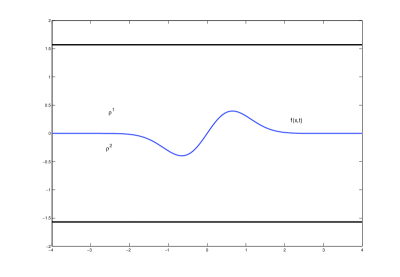
Let us consider the spatial domain for . We assume impermeable boundary conditions for the velocity in the walls. In this domain we have two immiscible and incompressible fluids with the same viscosity and different densities; fills the upper subdomain and fills the lower subdomain (see Figure 1). The graph is the interface between the fluids.
It is well-known that the system is in the (Rayleigh-Taylor) stable regime if the denser fluid is below the lighter one in every point , i.e. . Conversely, the system is in the unstable regime if there is at least a point where the denser fluid is above the lighter one.
If the fluids fill the whole plane the contour equation satisfies (see [11])
| (2) |
For this equation the authors show the existence of classical solution locally in time (see [11] and also [1, 14, 15, 19]) in the Rayleigh-Taylor stable regime, and maximum principles for and (see [12]). Moreover, in [4, 5] the authors show the existence of turning waves and finite time singularities. In [8] the authors show an energy balance for the norm and some results concerning the global existence of solutions corresponding to ’small’ initial data. Furthermore, they show that if initially , then there is global Lipschitz solution and if the initial data has small norm then there is global classical solution.
The case where the fluid domain is the strip , with , has been studied in [3, 13, 14, 15, 17]. In this domain the equation for the interface is
| (3) |
For equation (3) the authors in [13] obtain local existence of classical solution when the system starts its evolution in the stable regime and the initial interface does not reach the walls, and the existence of initial data such that blows up in finite time. The authors also study the effect of the boundaries on the evolution of the interface, obtaining the maximum principle and a decay estimate for and the maximum principle for for initial data satisfying the following hypotheses:
| (4) |
| (5) |
and
| (6) |
These hypotheses are smallness conditions relating , and the depth. We define as the solution of the system
| (7) |
Then, for initial data satisfying
| (8) |
the authors in [13] show that
These inequalities define a region where the slope of the solution can grow but it is bounded uniformly in time. This region only appears in the finite depth case.
In this paper the question of global existence of weak solution (in the sense of Definition 1) for (3) in the stable regime is adressed. In particular we show the following theorem:
Theorem 1.
Let be the initial datum satisfying hypotheses (4), (5) and (6) or (8) in the Rayleigh-Taylor stable regime. Then there exists a global solution
Moreover, if the initial data satisfy (4), (5) and (6) the solution fulfills the following bounds:
while, if the initial datums satisfy (8), the solution satisfies the following bounds:
This result excludes the formation of cusps (blow up of the first and second derivatives) and turning waves for these initial data, remaining open the existence (or non-existence) of corners (blow up of the curvature with finite first derivative) during the evolution. Notice that in the limit we recover the result contained in [8]. In this paper and the works [3, 13, 17] the effect of the boundaries over the evolution of the internal wave in a flow in porous media has been addressed. When these results for the confined case are compared with the known results in the case where the depth is infinite (see [5, 8, 11, 12]) three main differences appear:
-
1.
the decay of the maximum amplitude is slower in the confined case.
-
2.
there are smooth curves with finite energy that turn over in the confined case but do not show this behaviour when the fluids fill the whole plane.
-
3.
to avoid the turning effect in the confined case you need to have smallness conditions in and . However, in the unconfined case, only the condition in the slope is required. Moreover, in the confined case a new region without turning effect appears: a region without a maximum principle for the slope but with an uniform bound. In both cases (the region with the maximum principle and the region with the uniform bound), Theorem 1 ensures the existence of a global Lipschitz continuous solution.
Keeping these results in mind, there are some questions that remain open. For instance, the existence of a wave whose maximum slope grows but remains uniformly bounded, or the existence of a wave with small slope such that, due to the distance to the boundaries, its slope grows and the existence (or non-existence) of corner-like singularities when the initial data considered is small in .
The proof of Theorem 1 is achieved using some lemmas and propositions. First, we define ’ad hoc’ diffusive operators and the regularized system (see Section 2). For this regularized system, we show some a priori bounds for the amplitude and the slope. With these ’a priori’ bounds we show global existence of solution (see Section 3). Then, we obtain the weak solution to (3), , as the limit of the regularized solutions (see Sections 4 and 5).
Remark 1 On the rest of the paper we take and and we drop in the notation the dependence. We write for a universal constant that can change from one line to another. We denote
2 The regularized system
In this Section we define the regularized system and obtain some useful ’a priori’ bounds for the amplitude and the slope. To clarify the exposition we write for the solution of the regularized system.
2.1 Motivation and methodology
We remark that the term
in (3) is a singular integral operator, while
is not if the curve does not reach the boundaries. In order to remove the singularity while preserving the inner structure, we put a term for in both kernels. We define
| (9) |
and
| (10) |
To pass to the limit we use compactness coming from an uniform bound in
. Thus, we need to obtain ’a priori’ bounds for the amplitude and the slope. We define positive constants that will be fixed below depending only on the initial datum considered. Taking derivatives in , we obtain some terms with positive contribution. So, we attach some diffusive operators to the regularized system. Given a smooth function , we define
| (11) |
We notice that, if the depth is not , the previous operators should be rescaled and we write the subscript to keep this dependence in mind. These operators are finite depth versions of the classical . Roughly speaking, there are three different types of extra terms appearing in the derivatives of (9) and (10) that we need to control to obtain the ’a priori’ bound for the slope:
-
1.
There are terms which have an integrable singularity and they appear multiplied by . In order to handle these terms we add and . These two scales , , appear naturally due to the nonlinearity present in (3).
-
2.
There are terms which are nonlinear versions of and . These terms go to zero due to the convergence of the operators but they are not multiplied by . In order to handle these terms we add and .
-
3.
To absorb the nonsingular terms we add . We notice that, as , the square root converges to zero less than linearly. This factor will be used because the contribution of some terms is with .
Once the ’a priori’ bounds are achieved, we should prove global solvability in for the regularized system. To get this bound we add . We also regularize the initial datum. We take , and , a symmetric mollifier and define . Given we define the initial datum for the regularized system as
| (12) |
Putting all together, we define the regularized system
| (13) |
where are universal constants that will be fixed below depending only on the initial datum . We remark that for all . Notice that, due to the continuity of ,
uniformly on any compact set in . Since , we get and then, as as , we have a.e. Thus, we have and . Furthermore, we have that if satisfies the hypotheses (4), (5) and (6), also satisfy these hypotheses if is small enough. Moreover, if satisfy (8) the same remains valid for and if is small enough.
We use some properties of the operators . For the reader’s convenience, we collect them in the following lemma:
Lemma 1.
For the operators (see (11)), the following properties hold:
-
1.
is -symmetric.
-
2.
is positive definite.
-
3.
Let be a Schwartz function. Then, they converge acting on as goes to zero:
-
4.
Let be a Schwartz function. Then, the derivative can be written in two different forms as
Proof.
The proof of the first two statement follows from (11). For the proof of the third part we recall some useful facts: if , due to the Mean Value Theorem, we get
| (14) |
and
| (15) |
Now the proof follows in a straightforward way. For the last statement we use the cancellation coming from the principal value to define
Using the uniform convergence of the derivative, we conclude the result. ∎
2.2 Maximum principle for
In this section we prove an a priori bound for . To simplify notation we define
| (16) |
Proposition 1.
Proof.
Changing variables and taking the derivative we obtain that (13) is equivalent to
| (17) | |||||
If we define . Then we have (see [13] for the details). If we write and we get . We compute
By notational convenience we use the notation and we define
Evaluating (17) in we have
Using the definition of and classical trigonometric identities we have
Putting together all the terms in , we obtain
Assuming that , then and we obtain and . In the case , we have and we get and . Integrating this in time, we get
where in the last step we use the definition (12). In order to prove that the initial sign propagates we observe that if is positive (respectively negative) the same remains valid for . Assume now that and suppose that the line is reached (if this line is not reached at any time we are done). We write . We have , and we get and . If we denote . We have and . Integrating in time we conclude the result. ∎
2.3 Maximum principle for
In this section we prove an a priori bound for . We define
where and are defined in (16) and is a critical point for . We will use some bounds for and, for the reader’s convenience, we collect them in the following lemma:
Lemma 2.
Proof.
To prove this lemma we use the following splitting
Taylor’s theorem and the appropriate bounds using Proposition 1. ∎
First, we assume . Notice that we can take small enough to ensure that defined in (12) also fulfills the hypotheses (4), (5) and (6). From (17), taking one derivative and using Lemma 1, we get
| (23) | |||||
where is the integral corresponding to , is the integral corresponding to and
| (26) | |||||
This extra term appear from the regularization present in both .
We have
where
| (27) |
with
and
The second term is given by
| (28) |
where
We compute
with
| (29) |
where
and
The second term is given by
| (30) |
We need to obtain the local decay for . Assuming the classical solvability for (13) with an initial datum fulfilling the hypotheses (4), (5) and (6) we have that also fulfills (4), (5) and (6) if is small enough. Recall that and . The linear terms in (23) have the appropriate sign and they will be used to control the the positive contributions of the nonlinear terms. We need to prove that . For the sake of simplicity, we split the proof of this inequality in different lemmas.
Lemma 3.
If , we have
Proof.
This kind of terms will be absorbed by . We have to deal with . We start with the term corresponding to in (28). We write
Lemma 4.
If , we have
Proof.
We split
Since is small enough to ensure that the hypotheses (4), (5) and (6) hold at time , we have that, if ,
| (31) |
The term is not singular and can be bounded using (19) and (31):
We compute
with
and
Using the Mean Value Theorem, we bound the inner term as
Due to (31), the outer term is
Putting all together, we obtain
Then, using the diffusion given by to control , we get
Due to and , some terms have the appropriate sign:
thus we can neglect their contribution. Furthermore, we have
Taking and using the Mean Value Theorem, we get
Combining these terms we conclude this result. ∎
The term corresponding to in (28) is
Lemma 5.
If , we have
Proof.
The proof follows the same ideas as in Lemma 4. ∎
We are done with , thus, using the previous bound for , we are done with in (28). The terms in are not multiplied by and we have to obtain this decay from the integral. We write
Lemma 6.
We have
Proof.
We have
with
and
The term is not singular and can be bounded using (14) and (15) as follows:
We can bound in the same way,
We split the term as follows
where
and
To bound we need to use the diffusion coming from . Notice that, according to Lemma 1, we have
and, when evaluating in the point where reaches its maximum, the first two terms are positive and they can be neglected. We get
where in the last step we have used the previous splitting in and , (14) and (15). This concludes the result. ∎
Now that we have finished with , the term with is
We have
Lemma 7.
If , we have
Proof.
The proof is similar to the proof of Lemma 6 and, for the sake of brevity, omit it. ∎
In order to finish bounding in (27), we have to bound the term
This term, akin to the singular term in [13], is bounded using the hypotheses (4) and (5).
Proof.
Using classical trigonometric identities we can write
and
Therefore, as in [13], the sign of is the same as the sign of
The roots of are and , so, if we have
then we can ensure that this contribution is negative. Since (31), we get
Using the cancellation when , we obtain
| (32) |
where
We remark that . We consider the cases given by the sign and the size of .
1. Case : In this case, we have and . Using the definition of in (16) and the fact that , we have (20) (see Lemma 2). Notice that, in this case, we have and we get (21). Due to (20) and (21) we obtain
| (33) |
2. Case : In this case we have and . Therefore, we get and we can neglect it.
We are done with in (23) and now we move on to . These terms are easier because the integrals are not singular. With the same ideas as before we can bound the term involving :
Lemma 9.
The contribution of is bounded by
Proof.
The proof is straightforward. ∎
We are left with in (29). First, we consider
Lemma 10.
The term is bounded as
Proof.
Using classical trigonometric identities, we compute
| (35) |
∎
We have to bound the terms containing . These terms are
To obtain the decay with we split the integral in the regions and as before.
Lemma 11.
The terms and are bounded by
Proof.
We have the following result concerning the evolution of the slope:
Proposition 2.
Proof.
For the sake of simplicity we split the proof in different steps.
Step 1 (local decay): Combining in (32) and in Lemma 10, and using the bounds (33) and (35) and the hypothesis (6) we obtain
We take , , . Since we have a term and , we can compare the bounds in Lemmas 3- 11 with if is chosen big enough. The universal constant in all these bounds can be . We have shown that for every small enough, there is local in time decay. As is positive and arbitrary, we have
Step 2 (from local decay to an uniform bound): Then, in the worst case, we have
These inequalities ensure that the hypotheses (4), (5) and (6) hold at time and decays again.
Step 3 (the case where ): This case follows the same ideas, and we conclude, thus, the result. ∎
Proposition 3.
3 Global existence for
In this section we obtain ’a priori’ estimates in that ensure the global existence for the regularized systems (13) for initial data satisfying hypotheses (4), (5) and (6) or (8). First, notice that if the initial datum satisfies hypotheses (4), (5) and (6), by Propositions 1 and 2, the solution satisfies
| (36) |
If the initial datum satisfies (8), by Propositions 1 and 3, the solution to the regularized system again satisfies the bounds (36). Then we have the following proposition:
Proposition 4.
Proof.
We have to bound the norm of the function and its third derivative. We split the proof in different steps.
Step 0 (local existence): The local existence follows by classical energy methods as in [11, 13, 21].
Step 1 (the function): We have
Using (11) we get
and we obtain that the contribution of the linear terms is negative. The nonlinear term defined in (9) is
Using the cancellation coming from the principal value we have
Inserting (19) and (18) in the expression for we obtain
The second term in is
Using the Cauchy–Schwarz inequality, the equality and integrating by parts we get
To finish with the norm we have to deal with . We have
where is defined in (16). Using the same ideas as in and
we conclude the bound
Putting all these bounds together we get
| (37) |
Step 2 (the third derivative): To study the norm of the third derivative, we compute
The term is positive due to Lemma 1:
The nonlinear terms related to are
The term is not singular if and can be bounded using Hölder and Nirenberg interpolation inequalities. For the sake of brevity, we write some terms detailedly, being the rest analogous to them. We have
Using
we obtain
The second term is
and using the classical interpolation inequality
we get
We split the term as follows
These terms are not singular because of the domain of integration. We have to deal with the integrability at infinity in . We compute
The integrability at infinity is obtained using (14) and (15). We only bound the more singular terms in and . The most singular term in is
Using (14), (15) and (18), we obtain
Analogously, the more singular term in is
Using the same bounds as in , we get
Using classical trigonometric identities, we obtain
And the most singular term in is
Using the cancellation of the principal value integral we obtain
thus,
Integrating by parts in , we obtain the required decay at infinity and we conclude
Putting all together, we get
The nonlinear terms related to are
We observe that, due to and , this integral is not singular. Thus the inner part can be bounded following the same ideas as for . The integrability at infinity is obtained with the following splitting
The term is
and it can be handled as . The terms and have a term and they can be bounded following the steps in and by using (14) and (15). Putting all the estimates together we obtain
Using (37), Young’s inequality and the dissipation given by the Laplacian we get the ’a priori’ estimate
| (38) |
A classical continuation argument shows the global existence. ∎
4 Convergence of
In this section we study the limit of as .
Lemma 12.
Proof.
First, notice that, due to Propositions 1, 2 and 3 and hypotheses (4), (5) and (6), the regularized solutions satisfy
while, if the initial datum, instead of hypotheses (4), (5) and (6), satisfies (8) then
Due to the Banach-Alaoglu Theorem, these bounds imply that there exists a subsequence such that
and
with , any and every . Fixing , due to the uniform bound in and the Ascoli-Arzela Theorem we have that, up to a subsequence, uniformly on any bounded interval . Moreover, for all , we have
In order to prove this uniform convergence on compact sets we use the spaces and results contained in [8]. For , we define the norm
| (39) |
We define the Banach space as the completion of with respect to the norm (39). We have
The embedding is continuous and, due to the Ascoli-Arzela Theorem, the embedding is compact. We use the following Lemma
Lemma 13 ([8]).
Consider a sequence that is uniformly bounded in the space . Assume further that the weak derivative is in (not necessarily uniform) and is uniformly bounded in . Finally suppose that . Then there exists a subsequence of that converges strongly in
Due to this Lemma we only need to bound in (not uniformly) and in (uniformly). Using that , the linear terms in (17) can be bounded easily with a bound depending on . To bound the nonlinear terms we split the integral
and we compute
where we have used , (15), (18) and
The second term with the kernel involving is
The terms with the kernel involving are not singular and can be bounded following the same ideas
and
Putting together all these estimates we get
thus we conclude with the bound in .
To obtain the bound in we extend by zero outside of this ball of radius . Then, using Lemma 1, we integrate by parts and obtain
and
Using
we bound the linear terms in (8) as
being a universal constant. The nonlinear terms are
and
Using the boundedness of , we get
The outer part is not singular and can be bounded (as it was done before) applying . We get
Putting together all these bounds we obtain
Using Lemma 13, we conclude the result. ∎
5 Convergence of the regularized system
Looking at (3) we give the following definition
Definition 1.
is a weak solution of (3) if, for all the following equality holds
In this section we show the convergence, as , of the weak formulation (see Definition 1) of the problem (13).
Proposition 5.
Let be the limit of the regularized solutions . Then is a weak solution of (3).
Proof.
First, we deal with the linear terms. Using the weak-* convergence in and Lemma 1, we obtain
and
where, in the last step, we use the dominated convergence theorem and the convergence of the mollifier. To deal with the nonlinear terms we split the integrals
for sufficiently small and large enough . These parameters, , that will be fixed below, can depend on but they don’t depend on . For the inner part of the integrals, we get
The outer integral goes to zero as grows. We compute
As , the integrals are not singular and we only have to deal with the decay at infinity. Using (14), (15), (17), the bound , integrating by parts and using the extra decay coming from the principal value at infinity (see, for instance, the term in Proposition 4 in Section 3), we have
The only thing to check is the convergence of . Due to the compactness of the support of , we have
with large enough to ensure . Since we have (up to a subsequence) that uniformly on compact sets (see Lemma 12), the uniform convergence if and the continuity of all the functions in this integral, the limit in and the integral commute and we get
We conclude the proof of the Theorem 1 by taking and to control the tails and then we send . ∎
References
- [1] D. Ambrose. Well-posedness of two-phase Hele-Shaw flow without surface tension. European Journal of Applied Mathematics, 15(5) (2004) pp. 597-607.
- [2] J. Bear. Dynamics of fluids in porous media. Dover Publications, 1988.
- [3] L.C. Berselli, D. Córdoba and R.Granero-Belinchón. Local solvability and turning for the inhomogeneous Muskat problem. To appear in Interfaces and Free Boundaries. Preprint arXiv:1311.2194 [math.AP], 2012.
- [4] A. Castro, D. Cordoba, C. Fefferman, and F. Gancedo. Breakdown of smoothness for the Muskat problem. Archive for Rational Mechanics and Analysis, 208(3) (2013) pp. 805-909.
- [5] A. Castro, D. Cordoba, C. Fefferman, F. Gancedo, and M. Lopez-Fernandez. Rayleigh-taylor breakdown for the Muskat problem with applications to water waves. Annals of Math, 175, (2012), pp. 909-948.
- [6] M. Cerminara and A. Fasano. Modelling the dynamics of a geothermal reservoir fed by gravity driven flow through overstanding saturated rocks. Journal of Volcanology and Geothermal Research, Volume 233, (2012) pp. 37-54.
- [7] C. Cheng, D. Coutand, and S. Shkoller. Global existence and decay for solutions of the Hele-Shaw flow with injection. preprint arXiv:1208.6213 [math.AP], 2012.
- [8] P. Constantin, D. Cordoba, F. Gancedo, and R. Strain. On the global existence for the Muskat problem. Journal of the European Mathematical Society, 15, (2013), pp. 201-227.
- [9] P. Constantin and M. Pugh. Global solutions for small data to the Hele-Shaw problem. Nonlinearity, 6, (1993), pp. 393-415.
- [10] A. Cordoba, D. Córdoba, and F. Gancedo. Interface evolution: the Hele-Shaw and Muskat problems. Annals of Math, 173, no. 1:477–542, 2011.
- [11] D. Córdoba and F. Gancedo. Contour dynamics of incompressible 3-D fluids in a porous medium with different densities. Communications in Mathematical Physics, 273(2) (2007), pp. 445-471.
- [12] D. Córdoba and F. Gancedo. A maximum principle for the Muskat problem for fluids with different densities. Communications in Mathematical Physics, 286(2), (2009) pp. 681-696.
- [13] D. Córdoba, R. Granero-Belinchón and R. Orive. On the confined Muskat problem: differences with the deep water regime. Communications in Mathematical Sciences. 12(3), (2014) pp. 423-455.
- [14] J. Escher, A. Matioc, and B. Matioc. A generalized Rayleigh–Taylor condition for the Muskat problem. Nonlinearity, 25(1) (2011), pp. 73-92.
- [15] J. Escher and B. Matioc. On the parabolicity of the Muskat problem: Well-posedness, fingering, and stability results. Z. Anal. Anwend. 30, 193–218, 2011.
- [16] J. Escher and G. Simonett. Classical solutions for Hele-Shaw models with surface tension. Advances in Differential Equations, 2(4), (1997), pp. 619-642.
- [17] J. Gómez-Serrano and R.Granero-Belinchón. On turning waves for the inhomogeneous Muskat problem: a computer-assisted proof. To appear in Nonlinearity. Preprint arXiv:1311.0430 [math.AP], 2013.
- [18] H. Hele-Shaw. Flow of water. Nature, 58(1509), (1898), pp. 520-520.
- [19] H. Kawarada and H. Koshigoe. Unsteady flow in porous media with a free surface. Japan Journal of Industrial and Applied Mathematics, 8(1), (1991), 41-84.
- [20] H. Knüpfer and N. Masmoudi. Darcy flow on a plate with prescribed contact angle—well-posedness and lubrication approximation. preprint arXiv:1204.2278 [math.AP].
- [21] A. Majda and A. Bertozzi. Vorticity and incompressible flow. Cambridge Univ Pr, 2002.
- [22] M. Muskat. The flow of homogeneous fluids through porous media. Soil Science, 46(2), 1938.
- [23] D. Nield and A. Bejan. Convection in porous media. Springer Verlag, 2006.
- [24] M. Siegel, R. Caflisch, and S. Howison. Global existence, singular solutions, and ill-posedness for the Muskat problem. Communications on Pure and Applied Mathematics, 57(10) (2004), pp. 1374-1411.