Non-universal disordered Glauber dynamics

Abstract

We consider the one-dimensional Glauber dynamics with coupling disorder in terms of bilinear fermion Hamiltonians. Dynamic exponents embodied in the spectrum gap of these latter are evaluated numerically by averaging over both binary and Gaussian disorder realizations. In the first case, these exponents are found to follow the non-universal values of those of plain dimerized chains. In the second situation their values are still non-universal and sub-diffusive below a critical variance above which, however, the relaxation time is suggested to grow as a stretched exponential of the equilibrium correlation length.

I Introduction

In the absence of general principles accounting for the evolution of non-equilibrium systems, kinetic Ising models have been used to characterize a large variety of slow non-equilibrium processes Marro ; Privman . Among the most ubiquitous of these latter, the coarsening dynamics after a sudden quench from a disordered phase at high temperatures to an ordered one below the critical point still remains a subject of much interest and debate Bray . For pure substrates it is by now established that coarsening domains are characterized by a single time-dependent length scale growing as $t^{1/z}$, where $z$ is the dynamic exponent of the universality class to which the dynamics belongs. Depending on whether or not the order parameter is preserved by this latter, e.g. Kawasaki Kawa or Glauber Glauber dynamics, the network of (ferromagnetic) domains will coarsen respectively according to a sub-diffusive Lifshitz-Slyozov growth ($z=3$, see however Ref.Grynberg  ), or following a plain diffusive Allen-Cahn behavior ($z=2$)  Bray .

On the other hand, the case of coarsening systems with quenched disorder substrates modelling the effects of various experimental situations has also received considerable attention Bray ; Huse , especially in the context of random field and random bond Ising models Forgacs ; Biswal ; Paul ; Corberi ; Lippiello . In general, it is expected that quenched impurities play the role of energy barriers slowing down coarsening domains, the boundaries of which move by thermal activation over the landscape of these trapping centers Huse . However, it is not yet clear whether universal growth can take place at late evolution stages in the presence of strong disorder. Recent Monte Carlo simulations Lippiello of the Glauber dynamics using random ferromagnetic couplings drawn from uniform probability distributions suggest that after long pre-asymptotic crossovers the final growth in one dimension (1D) recovers the usual diffusive behavior referred to above, while becoming logarithmically slow in the two-dimensional case. For the 1D situation this is somehow intriguing as already at the level of a plain alternating-bond or dimerized chain Droz the dynamic exponents are known to be non-universal and sub-diffusive ($z>2$).

As part of the ongoing efforts in this context, here we revisit the 1D Glauber disordered dynamics in terms of bilinear fermion fields associated to the kinetics of its kinks or domain walls. Here, we rather focus on the dynamic exponent characterizing the actual growth of relaxation times $\tau$ with equilibrium correlation lengths $\xi$, which according to critical dynamic theories Hohenberg should scale as $\tau\propto\xi^{x}$ . But it is known Privman ; Menyhard that this latter exponent coincides with $z$ because at times comparable with $\tau$ the average domain size becomes of order $\xi$, so both descriptions are ultimately equivalent at large scales of space and time. The idea is to avoid the problem of dealing with prohibitively long transient regimes by pinpointing directly the relaxation time embodied in the spectrum gap of the evolution operator which, for that purpose, will be constructed and diagonalized in a domain wall representation. Although the critical point is strictly zero, the analysis is kept within low temperature regimes (with $\xi$ and $\tau$ becoming both arbitrarily large there), otherwise the dynamics would be rapidly arrested Derrida owing to the proliferation of large quantities of metastable states. The disorder considered throughout may include either exchange couplings of a single type (ferro or antiferromagnetic) or mixed ones, though as we shall see in a moment, the dynamics of these situations can be mapped onto each other via a simple spin transformation.

The outline of this work is organized as follows. In Sec. II we describe the basic kinetic steps under random spin exchanges using a kink or dual representation, and write down the underlying Glauber generator in quantum spin notation. Exploiting detailed balance Kampen we then recast this latter operator in terms of bilinear and symmetric fermion forms, thus allowing to evaluate its spectra through the solution of a secular problem whose dimensions grow linearly with the system size. In Sec. III we present the results arising from the numerical diagonalizations of this problem both for binary and Gaussian disorder realizations. Non-universal dynamic exponents as well as scaling forms drawn from the exact solution of the dimerized chain are then proposed and seen to be consistent with some of our numerical findings. However, when the width of the Gaussian disorder exceeds a certain threshold the relaxation time grows in a rather different (non-power-law) and much faster form. We close with Sec. IV which contains a recapitulation along with brief remarks on open issues and possible extensions of this work.

II Dynamics and bilinear forms

Let us consider the Glauber dynamics of the Ising chain Hamiltonian ${\cal H}=-\sum_{i}\,J_{i}\,S_{i}\,S_{i+1}\,$ with $L$ spins $S_{i}=\pm 1\,$ and disordered couplings $J_{i}$ chosen arbitrarily with any sign and strength. Unless stated otherwise, periodic boundary conditions (PBC) will be used throughout. The system is in contact with a heat bath at temperature $T$, which causes the states $|S\,\rangle=|S_{1},\,\dots\,,S_{L}\rangle$ to change by random flipping of single spins. The probability per unit time $W(S_{i}\to-S_{i})$ or transition rate for the $i$-th spin to flip is set to satisfy detailed balance Kampen (see below), so that the system relaxes to equilibrium. As is known, the simplest choice of rates complying with this condition corresponds to that of Glauber Glauber

$$W(S_{i}\to-S_{i}) = \alpha\left[\,1\,-\,\frac{S_{i}}{2}\,\left(\,\gamma_{i}^{-}\,S_{i-1}\,+\,\gamma_{i}^{+}\,S_{i+1}\,\right)\,\right]\,,$$

$$\gamma_{i}^{\pm} \equiv \tanh\left(K_{i}+K_{i-1}\right)\pm\tanh\left(K_{i}-K_{i-1}\right)\,,$$ (1)

where $K_{i}\equiv J_{i}/k_{B}T$, and the spin flip rate $\alpha$ is hereafter taken as $1/2$. We shall always measure the temperature in energy units; equivalently the Boltzmann constant $k_{B}$ is set to 1. Note that the nature of the dynamics is basically unaltered by whether some or all couplings are ferromagnetic ($J_{i}>0$) or antiferromagnetic ($J_{i}<0$). To check out rapidly this issue consider for simplicity a chain with open boundary conditions (just to avoid frustration due to eventual mismatch of antiferro exchanges), along with the mapping

$$R_{1}\equiv S_{1}\,,\;\;R_{i}\equiv S_{i}\,\prod_{n=1}^{i-1}{\rm sign}\left(J_{n}\right)\;\;{\rm for}\;\;1<i\leq L\,,$$ (2)

to new spins $R_{i}=\pm 1$. Then, to preserve the energy of the mapped configurations and therefore to maintain invariant all transition rates (these in turn depending on $\Delta{\cal H}/T$), clearly in the equivalent $R$-system all couplings must become ferromagnetic because $S_{i}\,S_{i+1}\to\,{\rm sign}\,(J_{i})\,R_{i}\,R_{i+1}$. In particular, the dynamics of the random $\pm J$ chain would then reduce to the homogeneous one. Also, notice that the single-spin flip dynamics maps onto itself. In that latter respect, this argumentation would not apply to the Kawasaki dynamics Kawa as owing to the exchange of $S$-pairs under antiferro couplings, the mapping (2) would then allow parallel $R$-pairs to flip.

Strictly, Ising Hamiltonians possess no intrinsic dynamics since all involved spin operators commute with one another. But when these systems are endowed with extrinsic transition rates $W(S\to S^{\prime})$, such as those of Eq. (1), their time evolution is described in terms of a Markovian process governed by a master equation Kampen . For our subsequent discussion it is convenient to think of this latter as a Schrödinger equation in an imaginary time

$$\partial_{t}|P(t)\,\rangle=-H\,|P(t)\,\rangle\,,$$ (3)

under a pseudo Hamiltonian or evolution operator $H$. This provides the probability distribution to find the system in a state $|P(t)\,\rangle\equiv\sum_{S}P(S,t)\,|S\,\rangle\,$ at time $t$, from the action of $H$ on a given initial distribution, i.e. $|P(t)\,\rangle=e^{-H\,t}\,|P(0)\,\rangle$. To ensure equilibrium at large times, the detailed balance condition referred to above simply requires that $P_{eq}(S)\,W(S\to S^{\prime})=P_{eq}(S^{\prime})\,W(S^{\prime}\to S),\;\forall\;|S\rangle,|S^{\prime}\rangle$. As usual, the diagonal and non-diagonal matrix elements of this Markovian operator are given respectively by

$$\langle\,S|H_{d}|S\,\rangle=\sum_{S^{\prime}\neq S}W(S\to S^{\prime})\,,\;\;\langle\,S^{\prime}|H_{nd}|S\,\rangle=-\,W(S\to S^{\prime})\,.$$ (4)

In particular, the first non-zero eigenvalue $E_{1}$ of such stochastic matrix singles out the relaxation time $\tau$ in which we are interested, i.e. $\tau=1/{\rm Re}\;E_{1}>0$, which is the largest characteristic time for any observable at a given low temperature. The case of $E_{0}=0$ just corresponds to the stationary mode.

In order to build up and diagonalize the operational analog of Eq. (4), in what follows it is convenient to work instead with the associated kink or domain wall dynamics rather than with the spin flipping process itself. Both representations are depicted schematically in Fig. 1.

Figure 1: Disordered transition rates [ Eq (5) ] for (a) creation-annihilation of kink pairs , and (b) hopping of kinks. These latter are denoted by vertical lines separating domains of opposite spin orientations.

Clearly from Eq. (1), the kink pairing and hopping rates indicated in this diagram become respectively

$$\epsilon_{{}_{\pm P_{i}}} = \left(\,1\pm\tanh P_{i}\right)/2\;\;\;,\,\;\;P_{i}=K_{i}+K_{i-1}\,,$$

$$\epsilon_{{}_{\pm Q_{i}}} = \left(\,1\pm\tanh Q_{i}\right)/2\;\;\;,\,\;\;Q_{i}=K_{i}-K_{i-1}\,.$$ (5)

Thus, if we think of the corresponding kink occupation numbers (0,1) as being related to usual spin-$\frac{1}{2}$ raising and lowering operators $\sigma^{+},\sigma^{-}$, we can directly identify the non-diagonal operators $H_{nd}\equiv H_{pairs}+H_{hops}$ associated to Eq. (4). Evidently, the transitions of these dual processes will be provided by

$$H_{pairs} = -\sum_{i}\,\left(\,\epsilon_{{}_{-P_{i}}}\,\sigma^{+}_{i-1}\,\sigma^{+}_{i}\,+\,\epsilon_{{}_{P_{i}}}\,\sigma^{-}_{i}\,\sigma^{-}_{i-1}\,\right)\,,$$ (6)

$$H_{hops} = -\sum_{i}\left(\,\epsilon_{{}_{-Q_{i}}}\,\sigma^{+}_{i}\,\sigma^{-}_{i-1}\,+\,\epsilon_{{}_{Q_{i}}}\,\sigma^{+}_{i-1}\,\sigma^{-}_{i}\,\right)\,.$$ (7)

On the other hand, a significant simplification arises for the diagonal terms needed for conservation of probability. The former basically count the number of hopping and pairing instances at which a given kink configuration can evolve to different ones in a single step. Although this would introduce two-body interaction terms of the form $\sigma^{+}_{i}\sigma^{-}_{i}\sigma^{+}_{i+1}\sigma^{-}_{i+1}$ it can be readily verified that their coefficients will all cancel out so long as the rates involved are those of Eq. (5), ultimately stemming from detailed balance. Thus, after some brief calculations we obtain

$$H_{d} = \sum_{i}\,\left(\,\epsilon_{{}_{-P_{i}}}+\,h_{i}\,\sigma^{+}_{i}\sigma^{-}_{i}\,\right)\,,$$

$$h_{i} = \big{(}\tanh Q_{i}+\tanh P_{i}+\tanh P_{i+1}-\tanh Q_{i+1}\big{)}/2\,,$$ (8)

and no kink interactions, irrespective of disorder in the original couplings. Also, it is worth remarking that since ultimately the signs of these latter do not affect the dynamics [ Eq. (2) ], at low temperatures and times much smaller than $t_{B}\simeq 2\min_{\,i}\,\{\,\left[1-\tanh\left(\,|K_{i}|+|K_{i-1}|\,\right)\right]^{-1}\}$ (say with all $J_{i}\neq 0$), these kink processes can then be seen as those of a set of annihilating random walks in a disordered media Cardy ; Odor ; us . Although in this analogy branching walks begin to appear at $t\gtrsim t_{B}$, yet there are some common aspects for both systems at large times (see concluding discussion).

To recast the non-diagonal parts of Eqs. (6) and (7) into a symmetric representation, we have recourse once more to detailed balance and rotate each $\sigma^{\pm}_{j}$ around the $z$ direction using imaginary angles $\phi_{j}=iK_{j}$. So, we consider the diagonal non-unitary similarity transformation $S=\exp\,(\,{1\over 2}\sum_{i}K_{i}\sigma^{z}_{i}\,)$ for which it is straightforward to show that

$$\sigma_{i}^{\pm}\;\sigma_{i-1}^{\pm} \to e^{\pm P_{i}}\;\sigma_{i}^{\pm}\;\sigma_{i-1}^{\pm}\,,$$

$$\sigma_{i}^{\pm}\;\sigma_{i-1}^{\mp} \to e^{\pm Q_{i}}\;\sigma_{i}^{\pm}\;\sigma_{i-1}^{\mp}\,,$$ (9)

besides keeping unaltered the algebra of $\sigma^{+}\!,\,\sigma^{-}\!$. After this pseudo spin rotation the above non-diagonal operators therefore transform as

$$H_{pairs} \to -\frac{1}{2}\,\sum_{i}\,{\rm sech}\,P_{i}\,\left(\,\sigma^{+}_{i}\,\sigma^{+}_{i-1}\,+{\rm H.\,c.}\,\right)\,,$$ (10)

$$H_{hops} \to -\frac{1}{2}\,\sum_{i}\,{\rm sech}\,Q_{i}\,\left(\,\sigma^{+}_{i}\,\sigma^{-}_{i-1}\,+\,{\rm H.\,c.}\,\right)\,,$$ (11)

while leaving Eq. (8) invariant. Thus, we are left with a bilinear Hermitian form whose spectrum gap embodies the wanted dynamic exponents referred to in Sec. I. In passing, it is worth mentioning that Eqs. (8), (10) and (11) also define an anisotropic $XY$ chain under both inhomogeneous couplings $J_{i}\!\!\phantom{.}^{{}^{X}_{Y}}=-\left({\rm sech}\,Q_{i}\pm{\rm sech}\,P_{i}\right)$ and transverse fields $h_{i}$. However, the commutation algebra of its constituents Pauli matrices, as well as that of the above raising and lowering operators, would complicate the analysis. Fortunately, since the parity of kinks is conserved throughout and all couplings extend just to nearest-neighbors, a Jordan-Wigner transformation to spinless fermions $c_{i}$ LSM enables us to progress further. With the aid of the real symmetric and antisymmetric tridiagonal $L\times L$ matrices (with boundaries) $A$ and $B$, defined respectively as

$$A = \left(\begin{array}[]{cccccc}h_{1}&x_{2}&0&\cdots&0&-x_{1}\\ x_{2}&h_{2}&x_{3}&\;\ddots&\phantom{\ddots}&0\\ 0&x_{3}&\phantom{a}\ddots&\ddots&\ddots&\vdots\\ \vdots&\,\ddots&\ddots&\ddots&x_{L-1}&0\\ 0&\phantom{\ddots}&\ddots&\;x_{L-1}&\;h_{L-1}&x_{L}\\ -x_{1}&\,0&\cdots&\;\;\;\;0^{\phantom{L^{L^{L^{2}}}}}&x_{L}&h_{L}\end{array}\right)\;,\;\;B=\left(\begin{array}[]{cccccc}0&y_{2}&0&\cdots&0&y_{1}\\ -y_{2}&0&y_{3}&\;\ddots&\phantom{\ddots}&0\\ 0&-y_{3}&\;\;\ddots&\ddots&\ddots&\vdots\\ \vdots&\ddots&\ddots&\ddots&y_{L-1}&0\\ 0&\phantom{\ddots}&\ddots&-y_{L-1}&0&y_{L}\\ -y_{1}&\,0&\cdots&\phantom{--}0^{\phantom{L^{L^{L^{2}}}}}&-y_{L}&0\end{array}\right)\,,$$ (24)

$$x_{i} \equiv -\frac{1}{2}\;{\rm sech}\,Q_{i}\;\;,\;\;y_{i}\equiv-\frac{1}{2}\;{\rm sech}\,P_{i}\,,$$ (25)

the Jordan-Wigner representation of spins finally lead us to the bilinear fermionic form

$$H=\sum_{i}\epsilon_{{}_{-P_{i}}}+\,\sum_{i,j}\,\left[\,c_{i}^{\dagger}\,A_{i,j}\,c_{j}\,+\,\frac{1}{2}\,\left(\,c_{i}^{\dagger}\,B_{i,j}\,c^{\dagger}_{j}\,+\,{\rm H.\,c.}\,\right)\,\right]\,.$$ (26)

The boundary matrix elements in $A$ and $B$ are especially aimed for PBC by respectively taking account of the contributions of $\sigma^{+}_{L}\sigma^{-}_{1}\to\,-c^{\dagger}_{L}\,c_{1}$ and $\sigma^{+}_{L}\sigma^{+}_{1}\to-\,c^{\dagger}_{L}\,c^{\dagger}_{1}$. Since the number of kinks $\sum_{i}\!\sigma^{+}_{i}\sigma^{-}_{i}\equiv\sum_{i}\!c^{\dagger}_{i}\,c_{i}$ under PBC is always even, only anticyclic conditions must be used in those boundary terms.

Following the standard literature LSM , this quadratic form can be recasted by means of a canonical (unitary) transformation into new $b_{n}$-fermions such that $\big{[}\,b_{n}\,,H\,\big{]}=E_{n}\,b_{n}$, and therefore

$$H=\frac{L}{2}\,+\,\sum_{n}\,E_{n}\Big{(}\,b^{\dagger}_{n}\,b_{n}-\frac{1}{2}\,\Big{)}\,.$$ (27)

Here, the additive constants are obtained by the invariance of the trace of $H$, whereas the eigenvalues $E_{n}$ of its elementary excitations are given by the solutions of either of the following two $L\times L$ secular equations LSM

$$\big{(}A\pm B\big{)}\,\big{(}A\mp B\big{)}\,\varphi^{\pm}_{n}=E^{2}_{n}\,\varphi^{\pm}_{n}\,.$$ (28)

Because $(A+B)^{T}=A-B$ the above products are symmetric and hence diagonalizable, both being in turn represented by real five-diagonal matrices (plus boundaries), as if they were single particle Hamiltonians with hoppings terms up to next-nearest neighbors. On the other hand, since by construction $H$ is a stochastic operator its vacuum energy always vanishes and therefore all eigenvalues should be constrained as $\sum_{n}E_{n}\equiv L,$ with $E_{n}>0$. This is an issue which we shall make use of as a consistency test in the numerical diagonalizations of Sec. III. The wanted relaxation time will then emerge by averaging the spectrum gap of this latter secular problem over several of its disorder realizations.

II.1 Dimerized case

Before continuing with the numerical analysis of Eq. (28) we pause to consider briefly the dynamics arising from a periodic array of $J_{1}$ - $J_{2}$ couplings over odd and even bonds, say. Equivalently, the above $P^{\prime}s$ and $Q^{\prime}s$ become $P\equiv K_{1}+K_{2}\,,\;Q\equiv K_{2}-K_{1}$. As already this situation is capable of yielding non-universal exponents Droz , it is instructive to see how these are recovered within the context discussed so far. We begin by Fourier transforming the $c_{i}$ operators of Eq. (26) to a set of wave fermions $f_{q}\,,\,g_{q}$

$$f_{q} = \sqrt{\frac{2}{L}}\;e^{-\,i\,q/4}\,\sum_{j=1}^{L/2}\,e^{-\,i\,qj}\,c_{2j-1}\,,$$

$$g_{q} = \sqrt{\frac{2}{L}}\;e^{\,i\,q/4}\,\sum_{j=1}^{L/2}\,e^{-\,i\,qj}\,c_{2j}\,,$$ (29)

with $L/2$ wave numbers

$$q\in{\cal Q}^{\pm}=\left\{\,\pm 2\,\frac{\pi}{L}\,,\pm 6\,\frac{\pi}{L}\,,\cdots\,,\pm(L-6)\,\frac{\pi}{L}\,,\pm(L-2)\,\frac{\pi}{L}\,\right\}\,,$$ (30)

accounting of the anticyclic conditions referred to above. The $e^{\pm\,i\,q/4}$ phase factors are just aimed at producing a real representation of $H$ when expressed in terms of $f$’s and $g$’s. After introducing the $2\times 2$ matrices,

$$A_{q}=\left(\begin{array}[]{cc}h^{-}\!\!&\;\;x_{q_{\phantom{1^{L}}}}\\ x_{q}\!\!&h^{+}\!\!\end{array}\!\!\!\!\right)\;,\;\;B_{q}=\left(\begin{array}[]{cc}0&y_{q_{\phantom{1^{L}}}}\\ y_{q}&0^{\phantom{L}}\end{array}\!\!\!\!\right)\,,$$

parametrized as

$$x_{q} = -\,{\rm sech}\,Q\,\cos\frac{q}{2}\,,\;\;y_{q}=-\,{\rm sech}\,P\,\sin\frac{q}{2}\,,$$ (31)

$$h^{\pm} = \tanh P\pm\tanh Q\,,$$

it is readily found that the problem splits into subspaces involving only the occupation numbers and pairing states of four fermions. Specifically, the dynamics is decomposed as

$$H=L\,\epsilon_{{}_{-P}}+\sum_{q\,\in\,{\cal Q}^{\pm}}H_{A}(q)\,+\,\frac{1}{2}\sum_{q\,\in\,{\cal Q}^{+}}\!\!\!H_{B}(q)\,,$$ (32)

where

$$H_{A}(q) = \big{(}\,f_{q}^{\dagger}\,,\,g_{q}^{\dagger}\,\big{)}\;A_{q}\,\left(\begin{array}[]{c}f_{q}\\ g_{q}\end{array}\right)\,,$$ (35)

$$H_{B}(q) = \big{(}\,f_{q}^{\dagger}\,,\,g_{q}^{\dagger}\,,\,f_{-q}^{\dagger}\,,\,g_{-q}^{\dagger}\,\big{)}\;\left(\begin{array}[]{cc}0&B_{q}\\ \!\!-B_{q}&0\end{array}\right)\,\left(\begin{array}[]{c}f^{{\dagger}^{\phantom{B}}}_{q}\\ g^{{\dagger}^{\phantom{B}}}_{q}\\ f^{{\dagger}^{\phantom{B}}}_{-q}\\ g^{{\dagger}^{\phantom{B}}}_{-q}\end{array}\!\right)\,+\,{\rm H.\,c.}\;,$$ (42)

which is the bilinear counterpart of Eq. (26) in this momentum space. Hence, the solution of the secular equation (28) here reduces to the diagonalization of either of the products $D_{q}^{\pm}\,D_{q}^{\mp}$ of the $4\times 4$ matrices

$$D_{q}^{\pm}=\left(\!\!\begin{array}[]{cc}A_{q}&\pm B_{q}\\ \pm B_{-q}&A_{-q}\end{array}\right)\,.$$ (43)

Thus after straightforward algebraic steps and taking the positive roots of the associated $E^{2}_{q}$ eigenvalues, we are ultimately lead to two elementary excitation bands, namely

$$E_{q}^{\pm} = 1\,\pm\,\sqrt{\,T^{+}\,+\,T^{-}\cos q\;}\,,$$

$$T^{\pm} = \left(\,\tanh^{2}P\pm\tanh^{2}Q\,\right)/2\,.$$ (44)

Parity conservation of original kinks allows to create only an even number of these excitations. Then, by occupying two $E^{-}_{q^{*}}$ levels with $q^{*}=\pm 2\pi/L$ when $|P|>|Q|$, or alternatively, using $q^{*}=\pm(L-2)\pi/L$ when $|P|<|Q|$, the spectrum gap $g=\tau^{-1}$ in the thermodynamic limit comes out to be

$$g=2\,\left(\,1-\tanh R\,\right)\,,\;\;R=\max\left(\,|P|\,,\,|Q|\,\right)\,,$$ (45)

On the other hand since in equilibrium all kinks become independent, the spin-spin correlation length is simply $\xi^{-1}=-{1\over 2}\ln\left(\,\tanh|K_{1}|\,\tanh|K_{2}|\,\right)$ Droz , thus growing as $\xi\sim e^{\,2|K_{1}|}$ in the low temperature regime, say for $|J_{2}|\geq|J_{1}|$. Therefore using Eq. (45) within that latter limit ($g\sim 4\,e^{-2R}$), we can now relate these two seemingly independent quantities via the non-universal dynamic exponents of Refs. Droz ; that is

$$\tau = \xi^{z}/\,4\,,$$

$$z = 1\,+\,|J_{2}/J_{1}|\;,\;{\rm for}\;\;|J_{2}|\geq|J_{1}|\,.$$ (46)

As expected from the simple but more general arguments given below Eq. (2), the role of the coupling signs is irrelevant.

Scaling regimes.– Finally, and in preparation for the finite-size scaling comparisons of Sec. III under both discrete and continuous disorder, it is helpful to consider also the spectrum gap of finite chains. Expanding the lower band of Eq. (44) to second order around either of the $q^{*}$ minima referred to above, and considering afterwards the scaling regime $L\to\infty,\,\xi\to\infty$ while holding $x\equiv\xi/L$ finite, it can be easily verified that the gap decay exhibits the crossover

$$g\propto\cases{\xi^{-z}\,\;\;\;\;\;\;\;\;\,{\rm for}\,\;\;x\ll 1/\pi\,,\cr\xi^{\,2-z}/L^{2}\,\;\;\;\;\;\;{\rm otherwise}\,.}$$ (47)

Evidently, this implies a typical Arrhenius dependence Privman for the relaxation time at low $T$’s, that is $\tau\propto\exp\,(2\,b/T)$ for $T/|J_{1}|\ll 1$, though now with energy barriers $b$ fixed by the interplay between temperatures and sizes, namely

$$b=\cases{|J_{2}|+|J_{1}|\;\;\;{\rm for}\,\;\;T/|J_{1}|\gg 1/\ln\sqrt{L}\,,\cr\cr|J_{2}|-|J_{1}|\;\;\;{\rm otherwise}\,.}$$ (48)

Moreover, both finite-size and finite correlation length corrections to these crossovers can also be estimated by keeping next leading order terms in Eq. (44). So, these finite effects are readily found to scale as

$$g\,\xi^{z}=4+4\pi^{2}\left(1-\frac{\,\pi^{2}}{3\,L^{2}}\right)x^{2}\,+\,{\cal O}\left(1/\xi^{z}\right)\,.$$ (49)

We will get back to these issues later on in the context of Figs. 3 and 4 of Sec. III.

III Numerical results

Turning to the diagonalization of Eq. (28), in what follows we consider the cases of binary and Gaussian probability distributions of disorder realizations, both taken site-independent. The coupling concentration ($p$) of the former is such that $P(J)=(1-p)\,\delta_{J,J_{1}}+p\,\delta_{J,J_{2}}$, whereas the latter is parametrized as usual by an average $\langle J\rangle$ and variance $\sigma^{2}\equiv\langle J^{2}\rangle-\langle J\rangle^{2}$. As the temperature is varied we focus on samples with correlation lengths close to their averaged disorder values, so as to minimize the dispersion of relaxation times resulting from finite-size effects. In the discrete case this is just equivalent to using a constant number of coupling types, i.e. the correlation length is fixed as $\xi_{p}=-\left[\,(1-p)\,\ln\left(\tanh|K_{1}|\right)+p\,\ln\left(\tanh|K_{2}|\right)\,\right]^{-1}$. For the continuous case, in turn we select and diagonalize only those samples having $\xi^{-1}=-\sum_{i}\ln\left(\,\tanh|K_{i}|\,\right)/L\simeq-\ln\left\langle\,\tanh|K|\,\right\rangle$, which amounts to work with disorder fixed (or nearly fixed) end-to-end spin-spin correlations.

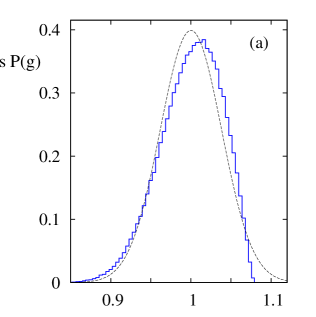
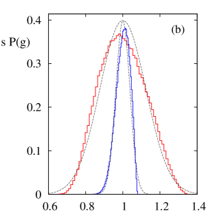
Figure 2: (Color online) Gap distributions over $3\times 10^{5}$ samples of $500$ spins after binning data in 70 intervals using (a) binary and, (b) Gaussian disorder realizations with fixed correlation length ($\xi\simeq L/2$). For comparison, dashed lines display Gaussian fittings with same mean and standard deviation ($s$) of otherwise skewed distributions. (a) illustrates the typical narrow dispersion $(s/\langle g\rangle\simeq 0.04)$ observed in the binary case (here, $T/|J_{1}|=0.36,\,|J_{2}/J_{1}|=2$, and $p=0.5$). In (b) an almost identical quantitative behavior is displayed for $\langle J\rangle=2$ with $T/\langle J\rangle=0.3$ and $\sigma/\langle J\rangle=0.15$ (innermost curve), whereas by contrast the case $T/\langle J\rangle=0.2$, $\sigma/\langle J\rangle=0.3>\bar{\sigma}_{c}$ (see text) but similar $\xi$, develops a more symmetric and broader dispersion $(s/\langle g\rangle\simeq 0.12)$.

In Fig. 2 we show the typical probability distributions of gaps arising from this simple procedure. Already for $500$ spins it is seen that standard gap deviations turn out to be fairly small. In particular, the abrupt decrease of these distributions above $g\gtrsim\langle g\rangle$ possibly signals the presence of natural upper bounds. However, for Gaussian disorders with $\sigma/\langle J\rangle\gtrsim 0.22$ (see below) but holding $\xi$ approximately constant (that is to say, choosing a temperature so as to keep comparable late domain sizes), this negative skewness is smeared out and the distributions widen significantly. As we shall see, at the level of average gaps this latter issue will be reflected in terms of a rather different decay of $\langle g\rangle$ with the correlation length. In averaging these gaps we used chains of up to 3000 spins for which the sampling had to be substantially reduced (down to 20 realizations). This is due to, in part, an $L^{3}$ increase of the diagonalization time of standard routines NR , as well as to a slowing down of convergence within low temperature or large $\xi$ regimes. The smallness of the spectrum gap for these regions and chain lengths also precluded us from using Lanczos-based algorithms Lanczos , as their convergence became even slower. Ultimately, these issues set the practical limit to the idea of singling out arbitrarily large relaxation times, as intended to in Sec. I.

III.1 Average binary gaps

Nonetheless, the relative errors of $\langle g\rangle$ yet remain small and clear trends emerge as $\xi$ is varied. Fig. 3 illustrates the resulting average decays for several parameter values of the binary distribution, all with $|J_{2}|>|J_{1}|$. It can be observed that within the very same scaling regime $\xi\lesssim L/\pi$ referred to in Eq. (47) for the plain dimerized chain, our results suggest a similar gap decay i.e. $\langle g\rangle\propto 1/\xi^{\,1\,+\,|J_{2}/J_{1}|}$, and irrespective of disorder concentrations Droz2 ; Robin .

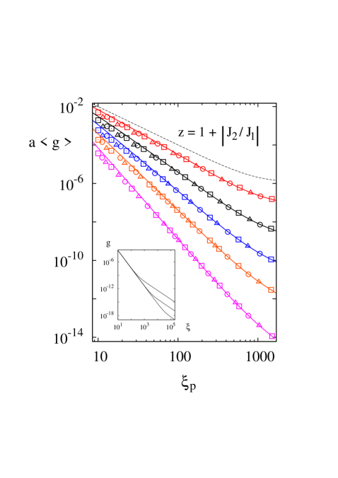
Figure 3: (Color online) Average gaps over 20 realizations of 3000 couplings drawn from binary distributions $(1-p)\,\delta_{J,J_{1}}+p\,\delta_{J,J_{2}}$. Squares, circles, and triangles refer respectively to concentrations $p=1/4,\,1/2,$ and 3/4 with correlation lengths $\xi_{p}$ as referred to in the text. Solid lines stand from top to bottom for dimerized cases with $\left|J_{2}/J_{1}\right|=1.5,\,2,\,2.5,\,3,$ and 3.75 ($\xi\equiv\xi_{p=1/2}$). Within the scaling region $\xi\lesssim L/\pi$, these closely follow the non-universal power law decays of their disordered counterparts, the gaps of which, for displaying purposes, have been normalized by different amplitudes. The inset illustrates the finite-size crossover mentioned in Eq. (47) for the dimerized situation using $L=10^{3}\!,10^{4}\!,10^{5}$ (top to bottom), and $\left|J_{2}/J_{1}\right|=3$ (also, see Fig. 4). For comparison, the uppermost dashed line in the main panel denotes the uniform case $z=2$.

Departures of data from this regime are equally followed by the exact solution of the alternating-bond chain, the finite-size aspects of which are depicted in the inset. Furthermore, as is shown in Fig. 4, above $\xi/L\sim 1/\pi$ the numerical diagonalizations also reproduce the universal scaling function contained in the thermodynamic limit of Eq. (49) (appart from an overall $p$ dependent amplitude), which therefore evidence the same crossover decay, i.e. $\langle g\rangle\propto\xi^{2-z}/L^{2}$, for the binary distribution.

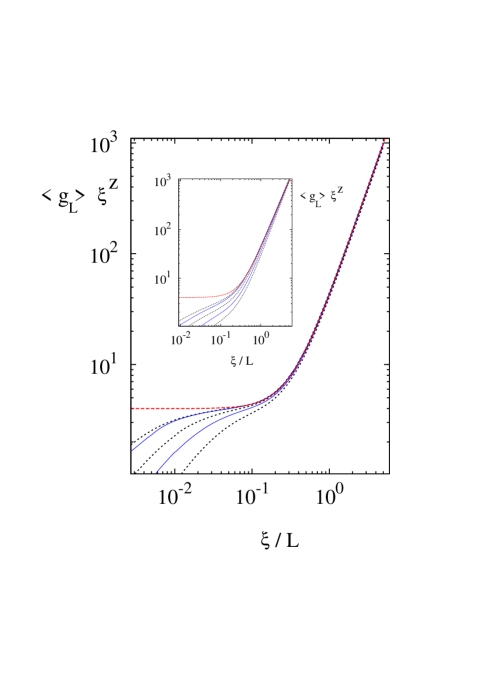
Figure 4: (Color online) Finite-size scaling regimes of average gaps and correlation lengths for a binary coupling disorder with $p=0.5$ and $\left|J_{2}/J_{1}\right|=2.5$ (main panel). From left to right doted and solid lines stand in turn for $L=3000,\,2000,\,1000,\,500,$ and 200. The data collapse in the scaling region $\xi/L\gtrsim 0.3$ is attained upon setting $z=1+\left|J_{2}/J_{1}\right|$. For much smaller values of $\xi/L$ finite-size departures show up with the same sign as those of Eq. (49), the thermodynamic limit of which is denoted by the dashed line. Similarly, the inset displays the scaling regimes of a Gaussian distribution with $\sigma/\langle J\rangle=0.15$ upon choosing $z\simeq 2.61$. For comparison with the above thermodynamic limit, all finite size data were rescaled by a common factor.

Alike the dimerized case, deviations from scaling are negligible within this region (all sizes yielding slopes $\simeq 2$), though as $\xi$ decreases subdominant $1/\xi^{z}$ corrections bring about breakdowns. Just as in Eq. (49), these happen to be of the same sign and more severe at the smaller sizes.

III.2 Average Gaussian gaps

Similar scaling features appear also for Gaussian disorder provided $\sigma$ is held small enough (see below), although finite-size departures become even more prominent for $\xi\lesssim L$, as is observed in inset of Fig. 4. In evaluating average gaps for this latter type of disorder, and in parallel with the behavior of the gap distributions referred to in Fig. 2b, two decay regimes are now obtained according to whether the relative standard deviation $\bar{\sigma}\equiv\sigma/\langle J\rangle$ is smaller or greater than a certain threshold $\bar{\sigma}_{c}$. This is displayed in Fig. 5a where we show some trends for 3000 spins using several variances for $\langle J\rangle=1$ and 2. As long as $\bar{\sigma}<\bar{\sigma}_{c}$ all gaps exhibit usual (but non-universal) power law decays $\propto 1/\xi^{z}$ with $z$ increasing slightly between 2 and $\sim$2.65 as $\bar{\sigma}$ increases. The incipient crossovers observed at $\xi\gtrsim 1000$ correspond to the scaling regimes already alluded to in the inset of Fig. 4, so there $\langle g\rangle\propto\xi^{2-z}$.

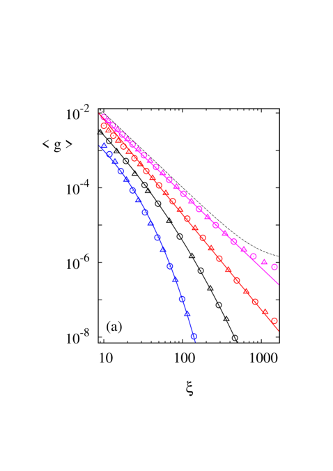
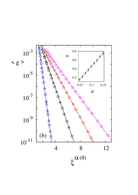
Figure 5: (Color online) Average spectrum gap for a Gaussian distribution of couplings over 20 samples of 3000 spins, all realization having in turn a common correlation length. In the main panels circles and triangles stand respectively for $\langle J\rangle=1$ and 2. From left to right each data set referrs to (a) $\bar{\sigma}\equiv\sigma/\langle J\rangle=0.3,\,0.25,\,0.2,\,0.1$ and, (b) $\bar{\sigma}=0.25,\,0.275,\,0.2875,\,0.3$. For $\bar{\sigma}<\bar{\sigma}_{c}\simeq 0.22$, in (a) data are fitted with non-universal power laws, whereas above such critical value all data closely follow stretched exponential decays [ Eq. (50) ] with stretching exponents $\alpha$ estimated as in the inset of (b). For comparison, dashed line in (a) denotes the ordered case $\sigma=0$.

By contrast, however, for $\bar{\sigma}>\bar{\sigma}_{c}$ a much faster decay emerges over the whole range of accessible correlation lengths, whereas the scaling relation put forward in Fig. 4 no longer holds. We direct the reader’s attention to Fig. 5b where it turns out that the non-linear least-squares fitting of the stretched exponential form

$$\langle g\rangle\sim A\,\exp\,\left(-\,a\,\xi^{\alpha}\right)\,,$$ (50)

is able to follow very closely all numerical diagonalizations. After estimating the stretching exponents of several variances it was found that above a threshold of $\bar{\sigma}_{c}\sim 0.22$ up to $\bar{\sigma}\sim 0.35$, they increase with $\bar{\sigma}$ as $\alpha\sim 6.01\,\left(\,\bar{\sigma}-\bar{\sigma}_{c}\right)$ as is shown in the inset of Fig. 5b. In nearing that critical variance however, it is difficult to distinguish the power law decay obtained before from this new behavior, so the crossover from one $\sigma$-regime to the other turns out to be smooth.

Let us mention that it would be important to elucidate whether this conjectured non-algebraic decay actually extends beyond the regions displayed in Fig. 5b, e.g. $\xi\lesssim$ 1500, 270 for $\bar{\sigma}=$ 0.25 and 0.3 respectively. However, above those correlation scales the numerical gaps get progressively smaller [ in turn resulting from the even smaller squared gaps of the secular problem (28) ], which brings about a much slower and erratic convergence of diagonalization routines NR .

IV Concluding discussion

Recapitulating, we have constructed a fermionic bilinear representation of the 1D Glauber dynamics with nearest-neighbor random interactions. This corresponds to the symmetric version [ Eq. (9) ] of the kink pairing and hopping processes schematized in Fig. 1. The relaxation time of these latter was reduced to the evaluation of the single-particle spectral gaps of the secular problem given in Eq. (28), the diagonalization of which ultimately led us to non-universal forms of domain growth. Some of these were expected and others not foreseen.

The case of binary disorder lent itself more readily for comparisons with the soluble alternating chain of same coupling types (Sec. II A). Although the former situation has no exact solution, based on decimation procedures as well as on simple diffusion arguments found in the literature Droz2 , the numerical coincidence of dynamic exponents with those of the soluble case should come as no surprise (Fig. 3). In addition, the scaling function of Eq. (49) reproduced our binary data just above regions displaying incipient departures from the actual exponents (Fig. 4, and rightmost part of Fig. 3). Because of this scaling robustness, the same barrier values involved in the crossover of Arrhenius times [ Eq. (48) ] might be expected to also hold in finite chains with binary disorder regardless of their bond concentrations. In passing, it is worth pointing out that such manifestation of finite-size effects has been observed experimentally in single-chain magnets Coulon .

Some of these scaling aspects seem to also apply for Gaussian disorder realizations with small relative variances (inset of Fig. 4), for which non-universal but yet power-law forms of gap decay were obtained (uppermost data in Fig. 5a). However, for $\sigma/\langle J\rangle\gtrsim 0.22$ a crossover to new regimes with much faster and non-algebraic decays showed up, whilst at the more detailed level of gap distributions this brought about a significant increase of dispersion (Fig. 2b). The stretched exponential form put forward to fit our data (Fig. 5b) lent further support to the former hypothesis which, by inverting Eq. (50) and recalling the large scale equivalences referred to in Sec. I Privman ; Menyhard , is tantamount to a dynamics of domain scales growing asymptotically as $\sim(\ln t)^{1/\alpha}$. Curiously, this rather slow form of phase-ordering kinetics is reminiscent to that conjectured and studied in late coarsening stages of higher dimensions with bond disorder Huse ; Lippiello . In turn, this behavior may be also viewed as that corresponding to a diverging dynamic exponent, somewhat analogous to activated scaling Fisher in random transverse-field magnets. The reason for such divergence is similar to that found in disordered reaction-diffusion processes thought of as annihilating random walks in a Brownian potential Cardy ; Odor ; us . The idea is that the equations of motion implicit in $\left[\,H\,,\,c_{l}\,\right]=\sum_{m}\left(\,A_{l,m}\,c_{m}\,+\,B_{l,m}\,c^{\dagger}_{m}\right)$ [ see Eqs. (24)-(26) ], can be mapped into a biased random walk of phase steps us whose first-passage probability to traverse a distance of order $\ln\tau$ sets a relationship between the dynamic exponent and the nonuniversal -disorder dependent- ratio $D/b$ (diffusion constant and bias of the random walk of phases). The limit of zero bias would then be related to an unbounded $z$-exponent and to a crossing over to the stretched exponential regime conjectured above us . As mentioned earlier on, at large times the analogy with annihilating random walks does not strictly apply but the reasoning in terms of steps of random phases goes along similar lines us (though here the mapping of the equations of motion couples the phase steps of two fields).

Alongside these growth law evaluations, it would be interesting to also address the issue of scaling and superuniversality (or the lack thereof), in two-time quantities such as autocorrelation and autoresponse functions Lippiello ; Henkel . That research line might well be further investigated with the fermion approach discussed in this work. Contrariwise, the effect of external fields Forgacs , whether random or not, would be bound to adopt rather cumbersome expressions had it been written in terms of the kink representation. For analogous reasons, the treatment of Glauber dynamics in higher dimensions remains beyond the scope of this approach.

References

- (1) J. Marro and R. Dickman, Nonequilibirum Phase Transitions in Lattice Models, (Cambridge University Press, 1999); P. Krapivsky, S. Redner and E. Ben-Naim, A Kinetic View of Statistical Physics, Chaps. 8 and 9 (Cambridge University Press, 2010).
- (2) Nonequilibrium Statistical Mechanics in One Dimension, edited by V. Privman, (Cambridge University Press, 1997).
- (3) For reviews, consult A. J. Bray, Adv. Phys. 43, 357 (1994); S. Puri, in Kinetics of Phase Transitions, edited by S. Puri and V. Wadhawan, (CRC Press, Boca Raton, 2009).
- (4) K. Kawasaki, Phys. Rev. 145, 224 (1966); K. Kawasaki in Phase Transitions and Critical Phenomena, edited by C. Domb and M.S. Green (Academic Press, London 1972), Vol. 2; S. J. Cornell, K. Kaski and R. B. Stinchcombe, Phys. Rev. B 44, 12263 (1991).
- (5) R. J. Glauber, J. Math. Phys. 4, 294 (1963) ; B. U. Felderhof, Rep. Math. Phys. 1, 215 (1971).
- (6) A somewhat slower growth was recently reported for the 1D Kawasaki dynamics. M. D. Grynberg, Phys. Rev. E 82, 051121 (2010).
- (7) D. A. Huse and C. L. Henley, Phys. Rev. Lett. 54, 2708 (1985); L. F. Cugliandolo, Physica A 389, 4360 (2010).
- (8) G. Forgacs, D. Mukamel and R. A. Pelcovits. Phys. Rev. B 30, 205 (1984); F. Corberi, A. de Candia, E. Lippiello and M. Zannetti, Phys. Rev. E 65, 046114 (2002).
- (9) B. Biswal, S. Puri and D. Chowdhury, Physica A 229, 72 (1996); M. A. Aliev, Physica A 277, 261 (2000).
- (10) R. Paul, S. Puri and H. Rieger, Europhys. Lett. 68, 881 (2004); Phys. Rev. E 71, 061109 (2005).
- (11) F. Corberi, E. Lippiello, A. Mukherjee, S. Puri and M. Zannetti, Phys. Rev. E 85, 021141 (2012).
- (12) E. Lippiello, A. Mukherjee, S. Puri and M. Zannetti, Europhys. Lett. 90, 46006 (2010); F. Corberi, E. Lippiello, A. Mukherjee, S. Puri and M. Zannetti, J. Stat. Mech. P03016 (2011).
- (13) M. Droz, J. Kamphorst Leal Da Silva and A. Malaspinas, Phys. Lett. A 115, 448 (1986); J. H. Luscombe, Phys. Rev. B 36, 501 (1987); see also S. J. Cornell in Ref.Privman .
- (14) P. C. Hohenberg and B. Halperin, Rev. Mod. Phys. 49, 435 (1977) .
- (15) N. Menyhárd, J. Phys. A 23, 2147 (1990).
- (16) B. Derrida and E. Gardner, J. Phys. (France) 47, 959 (1986); P. L. Krapivsky, J. Phys. I (France) 1, 1013 (1991).
- (17) N. G. van Kampen, Stochastic Processes in Physics and Chemistry, 3rd ed. (North Holland, Amsterdam, 2007).
- (18) M. J. E. Richardson and J. Cardy, J. Phys. A 32, 4035 (1999); P. Le Doussal and C. Monthus, Phys. Rev. E 60, 1212 (1999); G. M. Schütz and K. Mussawisade, Phys. Rev. E 57, 2563 (1998).
- (19) G. Ódor and N. Menyhárd, Phys. Rev. E 73, 036130 (2006); N. Menyhárd and G. Ódor, Phys. Rev. E 76, 021103 (2007).
- (20) M. D. Grynberg, G. L. Rossini and R. B. Stinchcombe, Phys. Rev. E 79, 061126 (2009).
- (21) E. Lieb, T. Schultz and D. Mattis, Ann. Phys. (NY) 16, 407 (1961), Appendix A; D. C. Mattis, The Theory of Magnetism Made Simple (World Scientific, Singapore, 2006), pages 474- 478.
- (22) Consult for instance, W.H. Press, S.A. Teukolsky, W.T. Vetterling and B.P. Flannery, Numerical Recipes, 2nd ed. (Cambridge University Press, 1992); see Chapter 11.
- (23) See for example, G. H. Golub and C. F. van Loan, Matrix Computations, 3rd ed., Chap. 9 (Johns Hopkins University Press, Baltimore, 1996); Y. Saad, Numerical Methods for Large Eigenvalue Problems, 2nd ed., Chap. 6 (SIAM, Philadelphia, 2011).
- (24) Consult the assumptions and arguments given by E. J. S. Lage, J. Phys. C 20, 3969 (1987); as well as those of M. Droz, J. Kamphorst Leal Da Silva, A. Malaspinas and A. L. Stella, J. Phys. A 20, L387 (1987).
- (25) The same exponents were also reported for the Fibonacci quasiperiodic chain with two coupling types, see J. A. Ashraff and R. B. Stinchcombe, Phys. Rev. B 40, 2278 (1989).
- (26) C. Coulon, R. Clérac, L. Lecren, W. Wernsdorfer and H. Miyasaka, Phys. Rev. B 69, 132408 (2004).
- (27) D. S. Fisher, J. Appl. Phys. 61, 3672 (1987); Phys. Rev. Lett. 69, 534 (1992); Phys. Rev. B 51, 6411 (1995).
- (28) M. Henkel and M. Pleimling, Europhys. Lett. 76, 561 (2006); Phys. Rev. B 78, 224419 (2008).