Saturation of the MRI in Strongly Radiation Dominated Accretion Disks

Abstract

The saturation level of the magneto-rotational instability (MRI) in a strongly radiation dominated accretion disk is studied using a new Godunov radiation MHD code in the unstratified shearing box approximation. Since vertical gravity is neglected in this work, our focus is on how the MRI saturates in the optically thick mid-plane of the disk. We confirm that turbulence generated by the MRI is very compressible in the radiation dominated regime, as found by previous calculations using the flux-limited diffusion approximation. We also find little difference in the saturation properties in calculations that use a larger horizontal domain (up to four times the vertical scale height in the radial direction). However, in strongly radiation pressure dominated disks (one in which the radiation energy density reaches $\sim 1\%$ of the rest mass energy density of the gas), we find Maxwell stress from the MRI turbulence is larger than the value produced when radiation pressure is replaced with the same amount of gas pressure. At the same time, the ratio between Maxwell stress and Reynolds stress is increased by almost a factor of $8$ compared with the gas pressure dominated case. We suggest that this effect is caused by radiation drag, which acts like bulk viscosity and changes the effective magnetic Prandtl number of the fluid. Radiation viscosity significantly exceeds both the microscopic plasma viscosity and resistivity, ensuring that radiation dominated systems occupy the high magnetic Prandtl number regime. Nevertheless, we find radiative shear viscosity is negligible compared to the Maxwell and Reynolds stress in the flow. This may have important implications for the structure of radiation dominated accretion disks.

1. Introduction

The inner regions of accretion disks around compact object are expected to be radiation pressure dominated (Shakura & Sunyaev, 1973; Pringle, 1981). Near the Eddington limit, the radiation field not only dominates the energy budget of the accretion disk, but also carries a significant fraction of the total momentum. The large accretion rate required to explain the observed X-ray luminosities of some compact objects cannot be explained by ordinary particle viscosity. Because the physical process to transfer angular momentum was unknown, Shakura & Sunyaev (1973) proposed the $\alpha$ disk model based on the assumption that the stress scales with the vertically integrated total pressure with a constant coefficient $\alpha$. Magneto-rotational instability (MRI) is now generally believed to be the physical mechanism to produce the required stress in ionized accretion disks (e.g., Balbus & Hawley, 1991, 1998). For the case with pure gas pressure, numerical simulations of MRI (e.g., Hawley et al., 1995; Stone et al., 1996; Miller & Stone, 2000) show that it saturates as a turbulent state and the Maxwell stress from the turbulence can reach $\sim 1\%$ — $10\%$ of the gas pressure. It is therefore important to understand how the MRI saturates in a radiation dominated flow. In particular, when the radiation energy density becomes a non-negligible fraction of the rest mass energy density of the gas, the properties of the MRI turbulence in the mid-plane of accretion disks may be affected by radiation, and radiative viscosity may contribute to the transport of angular momentum in this regime (e.g., Loeb & Laor, 1992).

A first step in studying the MRI in radiation pressure dominated disks was made by Turner et al. (2003), who studied MRI in the mid-plane of radiation dominated accretion disk using a flux-limited diffusion (FLD) module in ZEUS (Turner & Stone, 2001) and neglecting vertical gravity. The vertical structure of a stratified radiation dominated accretion disk was subsequently studied by Turner (2004), Hirose et al. (2009) and Blaes et al. (2011). One limitation of FLD is that it is based on single moment closure, and it drops radiation inertia in the momentum equation. When the accretion rate is near the Eddington limit, the photon momentum is a significant fraction of the fluid momentum, the FLD closure may not be appropriate to model the flow.

Recently, we have developed an improved algorithm for radiation MHD (see Jiang et al. 2012, thereafter JSD12 and Davis et al. 2012), based on a two-moment closure that solves the time dependent radiation momentum equations, and therefore retain radiation inertia. In this paper we use this algorithm to study the saturation of the MRI in the radiation dominated accretion disks. As a first step, we focus on the mid-plane of an accretion disk neglecting vertical gravity. Turner et al. (2003) found that for the parameters corresponding to the radiation dominated regime of the standard $\alpha$ disk model, the turbulence generated by MRI becomes highly compressible, consistent with expectation from the linear analysis (Blaes & Socrates, 2001). The Maxwell stress was found to be very similar to the value from simulations with radiation pressure replaced by the same amount of gas pressure. Here we attempt to reproduce these results without invoking the FLD approximation, as well as extend the study to higher ratios of radiation to gas pressure. The effects of the box size on the MRI turbulence will also be addressed (e.g., Bodo et al., 2008). In the case of gas pressure only, the properties of turbulence generated by the MRI have been studied extensively. For example, the ratio between Maxwell and Reynolds stress is always found to be $\sim 4-5$ Hawley et al. (1995); Blackman et al. (2008), and Maxwell stress is also found to scale with the magnetic pressure very well (e.g., Blackman et al., 2008; Guan et al., 2009; Hawley et al., 2011; Sorathia et al., 2012). Our goal is to investigate how these properties of MRI turbulence are affected by radiation, especially in a strongly radiation dominated flow.

This paper is organized as follows. In §2, we describe the equations we solve and the shearing periodic boundary condition we use, especially for the radiation quantities. Then in §3.1, we repeat and extend the fiducial simulations done by Turner et al. (2003). The saturation states of MRI for different total pressure are studied in §3.2. Discussions and conclusions are given in §4.

2. Equations

We adopt the local shearing box approximation with shearing periodic boundary conditions (e.g., Hawley et al., 1995) for this work. In this approximation, we solve the equations of motion in a frame rotating with orbital frequency $\Omega$ at a fiducial radius from the central black hole. Curvature is neglected and the equations are written in local Cartesian coordinates $(x,y,z)$ with unit vectors ($\bm{\hat{i}}$, $\bm{\hat{j}}$, $\bm{\hat{k}}$), which represent the radial, azimuthal and vertical direction respectively. Tidal and Coriolis forces are included in the local frame.

The implementation of the local shearing box approximation in Athena without radiation are described in detail by Stone & Gardiner (2010). For radiation MHD, we need to add radiation source terms as described by JSD12. The radiation MHD equations in the mixed frame under the local shearing box approximation are

$$\frac{\partial\rho}{\partial t}+{\mbox{\boldmath$\nabla$}}\cdot(\rho{\mbox{\boldmath$v$}}) = 0,$$

$$\frac{\partial(\rho{\mbox{\boldmath$v$}})}{\partial t}+{\mbox{\boldmath$\nabla$}}\cdot({\rho{\mbox{\boldmath$v$}}{\mbox{\boldmath$v$}}+{{\sf P}^{\ast}}}) = -{\bf\tilde{S}_{r}}({\mbox{\boldmath$P$}})$$

$$+ 2\rho\Omega^{2}qx\bm{\hat{i}}-2\Omega\bm{\hat{k}}\times\rho{\mbox{\boldmath$v$}},\$$

$$\frac{\partial{E}}{\partial t}+{\mbox{\boldmath$\nabla$}}\cdot\left[(E+P^{\ast}){\mbox{\boldmath$v$}}-{\mbox{\boldmath$B$}}({\mbox{\boldmath$B$}}\cdot{\mbox{\boldmath$v$}})\right] = -c\tilde{S}_{r}(E)$$

$$+ \Omega^{2}\rho{\mbox{\boldmath$v$}}\cdot(2qx\bm{\hat{i}}),$$

$$\frac{\partial{\mbox{\boldmath$B$}}}{\partial t}-{\mbox{\boldmath$\nabla$}}\times({\mbox{\boldmath$v$}}\times{\mbox{\boldmath$B$}}) = 0,$$

$$\frac{\partial E_{r}}{\partial t}+{\mbox{\boldmath$\nabla$}}\cdot{\mbox{\boldmath$F$}}_{r} = c\tilde{S}_{r}(E),$$

$$\frac{1}{c^{2}}\frac{\partial{\mbox{\boldmath$F$}}_{r}}{\partial t}+{\mbox{\boldmath$\nabla$}}\cdot{\sf P}_{r} = {\bf\tilde{S}_{r}}({\mbox{\boldmath$P$}}).$$ (1)

In the above equations, the shear parameter $q\equiv-d\ln\Omega/d\ln r$ and $q=3/2$ for Keplerian rotation while $\rho$ is density, ${\sf P}^{\ast}\equiv(P+B^{2}/2){{\sf\boldmath I}}$ (with ${{\sf\boldmath I}}$ the unit tensor), and the magnetic permeability $\mu=1$. The total gas energy density is

$$E=E_{g}+\frac{1}{2}\rho v^{2}+\frac{B^{2}}{2},$$ (2)

where $E_{g}$ is the internal gas energy density. We adopt the equation of state for an ideal gas with adiabatic index $\gamma=5/3$. Then $E_{g}=P/(\gamma-1)$ and $T=P/R_{\text{ideal}}\rho$, where $R_{\text{ideal}}$ is the ideal gas constant. Radiation pressure, energy density and flux are ${\sf P}_{r},\ E_{r}$ and ${\mbox{\boldmath$F$}}_{r}$ respectively while $c$ is the speed of light. The radiation momentum and energy source terms are ${\bf\tilde{S}_{r}}({\mbox{\boldmath$P$}})$ and $\tilde{S}_{r}(E)$.

Following Jiang et al. (2012), we use a dimensionless set of equations and variables in the remainder of this work. We convert the above set of equations to the dimensionless form by choosing fiducial units for velocity, density, temperature and pressure as $a_{0},\ \rho_{0},\ T_{0}$ and $P_{g,0}$ respectively. A dimensionless parameter ${\mathbb{P}}$ can be defined as ${\mathbb{P}}\equiv a_{r}T_{0}^{4}/P_{g,0}$, where $a_{r}$ is the radiation constant. Then units for radiation energy density $E_{r}$ and flux ${\mbox{\boldmath$F$}}_{r}$ are $a_{r}T_{0}^{4}$ and $ca_{r}T_{0}^{4}$. In other words, $a_{r}=1$ in our units. The dimensionless speed of light is ${\mathbb{C}}\equiv c/a_{0}$. The original dimensional equations can then be written to the following dimensionless form

$$\frac{\partial\rho}{\partial t}+{\mbox{\boldmath$\nabla$}}\cdot(\rho{\mbox{\boldmath$v$}}) = 0,$$

$$\frac{\partial(\rho{\mbox{\boldmath$v$}})}{\partial t}+{\mbox{\boldmath$\nabla$}}\cdot({\rho{\mbox{\boldmath$v$}}{\mbox{\boldmath$v$}}-{\mbox{\boldmath$B$}}{\mbox{\boldmath$B$}}+{{\sf P}^{\ast}}}) = -\mathbb{P}{\bf S_{r}}({\mbox{\boldmath$P$}})$$

$$+ 2\rho\Omega^{2}qx\bm{\hat{i}}-2\Omega\bm{\hat{k}}\times\rho{\mbox{\boldmath$v$}},\$$

$$\frac{\partial{E}}{\partial t}+{\mbox{\boldmath$\nabla$}}\cdot\left[(E+P^{\ast}){\mbox{\boldmath$v$}}-{\mbox{\boldmath$B$}}({\mbox{\boldmath$B$}}\cdot{\mbox{\boldmath$v$}})\right] = -\mathbb{PC}S_{r}(E)$$

$$+ \Omega^{2}\rho{\mbox{\boldmath$v$}}\cdot(2qx\bm{\hat{i}}),$$

$$\frac{\partial{\mbox{\boldmath$B$}}}{\partial t}-{\mbox{\boldmath$\nabla$}}\times({\mbox{\boldmath$v$}}\times{\mbox{\boldmath$B$}}) = 0,$$

$$\frac{\partial E_{r}}{\partial t}+\mathbb{C}{\mbox{\boldmath$\nabla$}}\cdot{\mbox{\boldmath$F$}}_{r} = \mathbb{C}S_{r}(E),$$

$$\frac{\partial{\mbox{\boldmath$F$}}_{r}}{\partial t}+\mathbb{C}{\mbox{\boldmath$\nabla$}}\cdot{\sf P}_{r} = \mathbb{C}{\bf S_{r}}({\mbox{\boldmath$P$}}),$$ (3)

where the source terms are,

$${\bf S_{r}}({\mbox{\boldmath$P$}}) = -\left(\sigma_{aF}+\sigma_{sF}\right)\left({\mbox{\boldmath$F$}}_{r}-\frac{{\mbox{\boldmath$v$}}E_{r}+{\mbox{\boldmath$v$}}\cdot{\sf P}_{r}}{\mathbb{C}}\right)$$

$$+ \frac{{\mbox{\boldmath$v$}}}{\mathbb{C}}(\sigma_{aP}T^{4}-\sigma_{aE}E_{r}),$$

$$S_{r}(E) = (\sigma_{aP}T^{4}-\sigma_{aE}E_{r})$$ (4)

$$+ (\sigma_{aF}-\sigma_{sF})\frac{{\mbox{\boldmath$v$}}}{\mathbb{C}}\cdot\left({\mbox{\boldmath$F$}}_{r}-\frac{{\mbox{\boldmath$v$}}E_{r}+{\mbox{\boldmath$v$}}\cdot{\sf P}_{r}}{\mathbb{C}}\right).$$

Frequency mean absorption and scattering opacities (attenuation coefficients) are $\sigma_{aF}$, $\sigma_{sF}$ respectively while $\sigma_{aP}$ and $\sigma_{aE}$ are Planck mean and energy mean absorption opacity (attenuation coefficients). To change the dimensionless equations to the dimensional form, we only need to replace ${\mathbb{C}}$ with $c$, set ${\mathbb{P}}=1$ and replace ${\mbox{\boldmath$F$}}_{r}$ with ${\mbox{\boldmath$F$}}_{r}/c$. Note that we solve the time-dependent radiation momentum equations, and therefore include radiation inertia effect.

The radiation pressure ${\sf P}_{r}$ is related to the radiation energy density $E_{r}$ with the variable Eddington tensor ${\sf\boldmath f}$:

$${\sf P}_{r}={\sf\boldmath f}E_{r}.$$ (5)

In principle, ${\sf\boldmath f}$ should be calculated with our short characteristic module as described by Davis et al. (2012). We have tried this approach and find that the difference between the Variable Eddington tensor (VET) and $1/3{{\sf\boldmath I}}$ is smaller than $10^{-4}$. Thus for unstratified disk simulations with uniform density in the optically thick regime, the Eddington approximation is adequate, and we will adopt it in this paper.

We use the recently developed Godunov radiation MHD method (JSD12) to solve those equations. This algorithm has been implemented and tested in Athena (Stone et al., 2008) as described in JSD12 with several improvements as explained in Appendix A. The momentum and energy source terms resulting from the shearing box approximation are added in the same way as in Stone & Gardiner (2010), which are separated from the radiation source terms.

2.1. Boundary Condition

We adopt the usual shearing periodic boundary condition in $x$, and periodic boundary condition in both $y$ and $z$ directions (e.g., Hawley et al., 1995). Boundary conditions for the gas quantities are the same as in non-radiative MHD simulations (e.g., Stone & Gardiner, 2010). The radiation quantities $E_{r}$ and ${\mbox{\boldmath$F$}}_{r}$ are new variables, and boundary conditions for them deserve detailed discussion.

If the radial size of the simulation box is $L_{x}$, then the boundary condition for $E_{r}$ is

$$E_{r}(x,y,z)\mapsto E_{r}(x\pm L_{x},y\mp q\Omega L_{x}t,z).$$ (6)

This boundary condition is the same as the boundary condition for density. ${\mbox{\boldmath$F$}}_{r}$ is the Eulerian radiation flux, which includes the co-moving and advected radiation flux. We first remap the co-moving radiation flux and then add the advection flux at the new location. Thus the boundary condition for ${\mbox{\boldmath$F$}}_{r}$ is

$$F_{r,x} \mapsto F_{r,x}(x\pm L_{x},y\mp q\Omega L_{x}t,z),$$

$$F_{r,y} \mapsto F_{r,y}(x\pm L_{x},y\mp q\Omega L_{x}t,z)$$

$$\mp (1+f_{yy})\frac{q\Omega L_{x}}{{\mathbb{C}}}E_{r}(x\pm L_{x},y\mp q\Omega L_{x}t,z),$$

$$F_{r,z} \mapsto F_{r,z}(x\pm L_{x},y\mp q\Omega L_{x}t,z),$$ (7)

where $f_{yy}$ is the $yy$ component of the Eddington tensor at the new location.

2.2. Energy Conservation

Unlike the ZEUS code, Athena conserves energy to roundoff error when energies exchange between kinetic, internal and magnetic forms. However, as explained in JSD12, when photons and gas exchange energy, the radiation module in Athena does not conserve total energy to round off error because of our splitting scheme and the implicit matrix solver. With the special treatment of the energy source term described in JSD12, the energy error is kept small. This is particularly important for MRI simulations because the gas is continuously heated up during the simulations. If the energy error is not treated carefully, it can accumulate and eventually affect the dynamics.

For unstratified simulations with shearing periodic boundary conditions, the change of the total energy inside the simulation box is entirely due to the work done on the walls (e.g., Hawley et al., 1995; Gardiner & Stone, 2005). With radiation, the volume averaged total energy is $E_{t}\equiv\langle E+\rho\Phi+{\mathbb{P}}E_{r}\rangle$, where $\Phi$ is the tidal potential $\Phi=-q\Omega^{2}x^{2}$. The change of total energy is determined by

$$\frac{\partial E_{t}}{\partial t}=\frac{q\Omega}{L_{y}L_{z}}\int_{X}\left(\rho v_{x}\delta v_{y}-B_{x}B_{y}\right)dydz\equiv W(t),$$ (8)

where $\delta v_{y}\equiv v_{y}+q\Omega x$, and the integral only needs to be done on one side of the radial boundary. The total work done on the simulation box within a certain time $t_{0}$ is then $W_{t}(t_{0})=\int_{0}^{t_{0}}W(t)dt$. To check the energy error, we calculate the energy change at $t_{0}$ as $\delta E=E_{t}(t_{0})-E_{t}(0)$, so that the energy error is $\delta E-W_{t}(t_{0})$. We calculate this energy error for all simulations and find that with respect to the total work $W_{t}(t_{0})$ within the first $100$ orbits, the energy errors are always smaller than $1\%$.

3. Results

In this section, we first repeat the fiducial simulations done by Turner et al. (2003) and then extend them to a box with a larger radial size. In addition, we will study the saturation state of MRI turbulence with different radiation pressure.

3.1. Simulations with Net Vertical Flux

Turner et al. (2003) used the FLD module in ZEUS (Turner & Stone, 2001) to study MRI turbulence in the optically thick regime of a unstratified disk model. The radial size of the simulation box was fixed to be one scale height. Here we repeat their simulations with net vertical flux to compare the results from the two different codes. Because the whole simulation box is very optically thick, we expect to find similar results as those computed with FLD. We also extend the radial size of the simulation box to four scale height to study possible new effects with radiation in this larger radial domain (e.g., Bodo et al., 2008).

3.1.1 Initial Condition

We take the parameters for location I in table 1 of Turner et al. (2003). This corresponds to a radius $67.8r_{G}$ from a $10^{8}M_{\odot}$ supermassive black hole, where the gravitational radius $r_{G}\equiv GM/c^{2}$ and $M$ is the black hole mass. The whole simulation box has uniform density $\rho_{0}=2.89\times 10^{-9}$ g cm^-3 and temperature $T_{0}=2.71\times 10^{5}$ K. The density and temperature correspond to the mid-plane in an $\alpha$ disk model with $\alpha=0.01$ and accretion rate $10\%$ of the Eddington rate. The mean molecular weight is assumed to be $0.6$. Gas and radiation are in thermal equilibrium initially. We include both electron scattering opacity $\kappa_{\rm T}=0.4$ cm² g^-1 and free-free absorption opacity $\kappa_{\rm ff}=10^{52}\rho^{9/2}\left[P_{g}/(\gamma-1)\right]^{-7/2}$ cm² g^-1. Taking the unit of density to be $\rho_{0}$, temperature to be $T_{0}$, pressure to be $P_{g,0}=\rho_{0}R_{\text{ideal}}T_{0}$ (with $R_{\text{ideal}}$ to be the ideal gas constant), time to be $1/\Omega$, and length to be $L_{0}=(P_{g,0}/\rho_{0})^{0.5}/\Omega$, the dimensionless parameters in our equations are ${\mathbb{P}}=376.3$, ${\mathbb{C}}=4895.6$, $\sigma_{sF}=1953.9$, and $\sigma_{aF}=\sigma_{aP}=\sigma_{aE}=0.105$. Thus the ratio between the background radiation and gas pressure is $\sim 125$. The ratio between radiation energy density and rest mass energy of the fluid is $a_{r}T_{0}^{4}/\left(\rho_{0}c^{2}\right)=3.14\times 10^{-5}$. Table 1 lists other parameters for the five simulations in this section, with different box sizes and resolutions.

The initial magnetic field is $B_{x}=B_{y}=0,B_{z}=0.0353$. The most unstable MRI wavelength is $\lambda_{z}=2\pi v_{A,z}/\Omega=2\pi\sqrt{B^{2}/\rho}/\Omega=0.22L_{0}$. Notice that with the unit of length we choose, the size of the simulation box are smaller than the fiducial runs done by Turner et al. (2003). The net magnetic vertical flux we use is also smaller so that the ratio between the most unstable MRI wavelength and the vertical size of the simulation box is the same as in Turner et al. (2003). We have found that choosing a smaller field strength produces less vigorous channel solutions (e.g., Goodman & Xu, 1994) and leads to a more rapid transition to turbulence. Initial random perturbations are applied to both gas pressure and velocity field

$$P_{g}=P_{g,0}(1+\delta_{1}),v_{x}=\delta_{2},v_{y}=\delta_{3}-q\Omega x,v_{z}=\delta_{4},$$ (9)

where $\delta_{1}$ is a random number uniformly distributed between $-0.1$ and $0.1$ while $\delta_{2},\delta_{3},\delta_{4}$ are random numbers uniformly distributed between $-0.02$ and $0.02$. Athena’s orbital advection scheme, as described in Stone & Gardiner (2010), is used for all the simulations to speed up the calculation. For the radiation field, the advective radiation flux due to the mean orbital motion is separated from other terms and added as described in Appendix A.2.

Table 1Parameters for simulations with net vertical flux

Label	$L_{x}/L_{0}$	Grids/$L_{0}$	$\tau_{s}$	$\tau_{a}$	$P_{g}$	$P_{r}$	$B_{z,0}^{2}/2$
ZFRS	1	32	1954	0.11	1	125	$6.25\times 10^{-4}$
ZFRL	4	32	1954	0.11	1	125	$6.25\times 10^{-4}$
ZFNRS	1	32	—	—	126	—	$6.25\times 10^{-4}$
ZFNRL	4	32	—	—	126	—	$6.25\times 10^{-4}$
ZFRS64	1	64	1954	0.11	1	125	$6.25\times 10^{-4}$

• $\tau_{s}$ is the electron scattering optical depth per $L_{0}$.

• $\tau_{a}$ is the Planck mean free-free absorption optical depth per $L_{0}$.

Table 2Temporal and Spatial Averaged Properties of Simulations with Net Vertical flux

Label	$\,\langle\langle-B_{x}B_{y}\,\rangle\rangle$	$\,\langle\langle\rho v_{x}\delta v_{y}\,\rangle\rangle$	$\,\langle\langle B^{2}/2\,\rangle\rangle$	$\,\langle\langle B_{x}^{2}/2\,\rangle\rangle$	$\alpha_{\text{stress}}$
ZFRS	0.154	0.0282	0.320	0.0398	5.46
ZFRL	0.162	0.0291	0.338	0.0530	5.57
ZFNRS	0.235	0.0347	0.518	0.0560	6.77
ZFNRL	0.123	0.0273	0.240	0.0390	4.51
ZFRS64	0.321	0.0486	0.761	0.137	6.71
Label	$\,\langle\langle B_{y}^{2}/2\,\rangle\rangle$	$\,\langle\langle B_{z}^{2}/2\,\rangle\rangle$	$\,\langle\langle T/T_{0}\,\rangle\rangle$	$\alpha_{\text{mag}}$	$\alpha$
ZFRS	0.268	0.0113	1.04	0.481	0.00145
ZFRL	0.263	0.0220	1.05	0.478	0.00151
ZFNRS	0.448	0.0150	1.61	0.453	0.00214
ZFNRL	0.188	0.0130	1.41	0.513	0.00119
ZFRS64	0.556	0.0683	1.09	0.428	0.00297

3.1.2 Time Evolution

The fiducial simulation in Table 1, ZFRS, has the standard geometry $L_{x}=L_{0},L_{y}=4L_{0},L_{z}=L_{0}$. To see the effect of the size of the simulation domain, we increase the radial size such that $L_{x}=4L_{0}$ and label this simulation ZFRL. For comparison, the simulations ZFRNS and ZFNRL have the same parameters as ZFRS and ZFRL respectively, except that radiation pressure is replaced with the same amount of gas pressure. The differences between the two sets of simulations will be due to the radiation field. Simulation ZFRS64 has double the resolution of ZFRS.

In Figure 1, we show the time evolution of radiation and gas pressure, three components of magnetic and kinetic energy densities as well as the total work done on the wall of the simulation box per unit time for the fiducial run ZFRS. Because photons cannot leave the system in the unstratified shearing box models, and moreover the box is continuously heated up due to the work done on the walls, there is no equilibrium solution and radiation and gas pressure continue to increase. Since $E_{r}\propto T^{4}$ while gas internal energy density $E_{g}\propto T$, radiation energy density increases faster and most of the work is converted to the radiation energy density. Although total energy cannot reach an equilibrium state, the magnetic and kinetic energy densities saturate quickly after the initial transient. They fluctuate around some mean values, which do not show any systematic change with pressure within the $100$ orbits. This is also true for the Maxwell and Reynolds stress, the histories of which for four simulations are shown in Figure 2. Time histories of these quantities are very similar for simulations with or without radiation and it is independent of the box size.

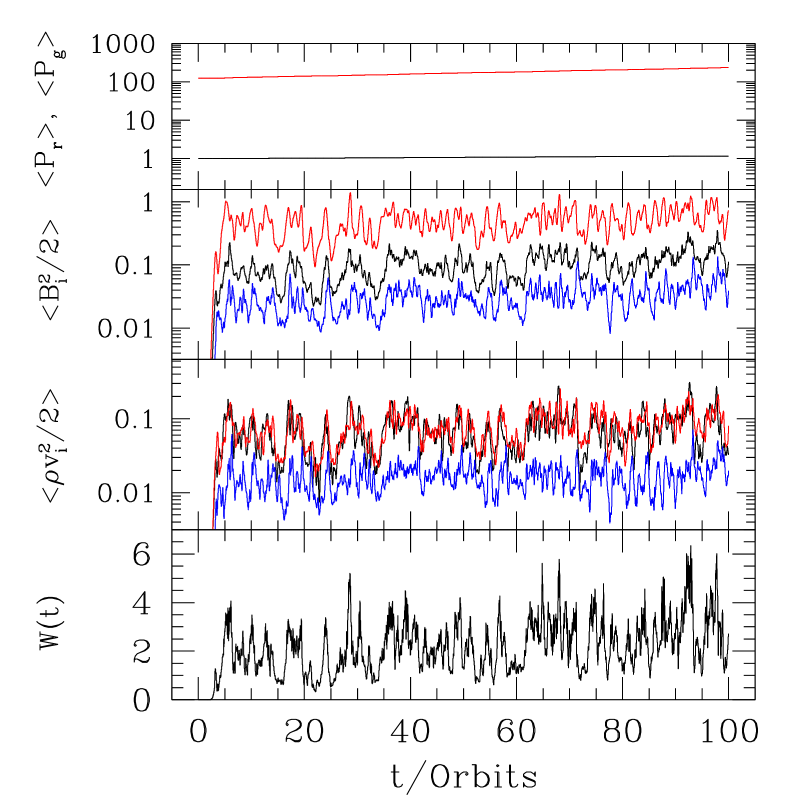
Figure 1.— Time history of the spatially averaged quantities from simulation ZFRS with net vertical flux. The radiation (the red line) and gas (the black line) pressure are shown in the top panel. Components of the magnetic and kinetic energy densities are shown in the middle two panels. The black, red and blue lines represent $x$, $y$ and $z$ components respectively. Background shearing is not included in the calculation of kinetic energy density. The bottom panel shows the total work done on the wall per unit time, calculated according to equation 8.

Figure 2.— History of the spatially averaged Maxwell stress (left panels) and Renolds stress (right panels) for the four simulations with net vertical flux. Parameters of the four simulations are given in Table 1. The stress is normalized with respect to the initial total pressure. The number in each panel is the time averaged value between 10 and 100 orbits.

3.1.3 Statistical Properties

In Table 2, we calculate different spatial and temporal averaged quantities for the five simulations. The temporal averages are taken between $10$ and $100$ orbits to avoid the initial transient before the MRI saturates. In that table, $\alpha_{\text{stress}},\alpha_{\text{mag}}$ and $\alpha$ are defined as

$$\alpha_{\text{stress}} \equiv \frac{\,\langle\langle-B_{x}B_{y}\,\rangle\rangle}{\,\langle\langle\rho v_{x}\delta v_{y}\,\rangle\rangle},\alpha_{\text{mag}}\equiv\frac{\,\langle\langle-B_{x}B_{y}\,\rangle\rangle}{\,\langle\langle B^{2}/2\,\rangle\rangle},$$

$$\alpha \equiv \frac{\,\langle\langle-B_{x}B_{y}+\rho v_{x}\delta v_{y}\,\rangle\rangle}{P_{0}},$$ (10)

where $P_{0}$ is the initial total pressure and $\,\langle\langle\cdot\,\rangle\rangle$ represents spatial and temporal averaging.

As shown in Table 2, the averaged Maxwell stress, Reynolds stress and magnetic pressure are very similar for simulations ZFRS and ZFRL, which suggests that changing the box size along radial direction does not affect the statistical properties of the turbulence. However, as shown in Figure 2, when $L_{x}$ is increased by a factor of $4$, there are fewer large spikes compared with the fiducial run. This is also true for the pure gas pressure runs (simulations ZFNRS and ZFNRL). This is consistent with Bodo et al. (2008) for MRI without radiation. The spikes in the fiducial run are due to the recurrent channel solutions. When the radial size is increased, the channel solution can be more easily destroyed either by the parasitic modes (e.g., Goodman & Xu, 1994; Pessah & Goodman, 2009), or by the interactions between different MRI modes (e.g., Latter et al., 2009).

When radiation pressure is replaced with the same amount of gas pressure, Maxwell stress for simulation ZFNRS is about $50\%$ larger than for simulation ZFRS. The difference is primarily due to the large spikes in the non-radiative run, which are weaker by almost a factor of $5$ for the simulation with radiation. If we exclude those spikes, ZFNRS has a very similar saturation level as ZFRS. The change in temperature is $50\%$ larger during the first $100$ orbits for ZFNRS than ZFRS, although the total work done on the fluid is very similar for the two simulations. This is because the heat capacity for the photons is much larger than an ideal gas. When $L_{x}$ is increased by a factor of $4$, ZFNRL and ZFRL have roughly the same Maxwell stress and Reynolds stress. This is consistent with Figure 2 of Turner et al. (2003), which shows that the stress is very similar when the net vertical flux and total pressure are the same for their simulations NV4 and RV4. The stresses from our simulations are smaller than what Turner et al. (2003) found because we use a smaller net vertical flux. This is roughly consistent with the scaling between the saturated Maxwell stress and the initial net vertical magnetic flux as found by Hawley et al. (1995). Simulations RV4h, RV4 and RV4l in Turner et al. (2003) also have very similar stress, although the three simulations have quite different opacities and thus different coupling between the photons and gas.

The ratio between Maxwell and Reynolds stress, $\alpha_{\text{stress}}$, varies from $4.5$ to $6.8$ for the first four simulations in Table 2. This is also consistent with previous MRI simulations with (e.g., Turner et al., 2003) or without (e.g., Sano et al., 2004; Davis et al., 2010) radiation. When resolution is doubled for simulation ZFRS64, the Maxwell stress is doubled while Reynolds stress is increased by $70\%$ compared with simulation ZFRS. But the ratio between Maxwell stress and magnetic pressure $\alpha_{\text{mag}}$ varies in the small range $0.43\sim 0.51$ for all the five simulations. This is consistent with previous work, which found $\alpha_{\text{mag}}$, or the tilt angle defined based on it (e.g., Guan et al., 2009; Hawley et al., 2011; Sorathia et al., 2012), to be roughly constant for converged simulations with different box sizes and initial conditions (e.g., Blackman et al., 2008; Hawley et al., 2011). Most previous MRI simulations without radiation find $\alpha_{\text{mag}}\sim 0.5$ (e.g., Guan et al., 2009), although a range of $0.3-0.4$ is also reported by Hawley et al. (2011) for the stratified disk simulations.

3.1.4 Density fluctuation

When there is no radiation field, turbulence generated by the MRI is almost incompressible. However, Turner et al. (2003) finds that if the photon diffusion length per orbit is larger than the most unstable MRI wavelength, the turbulence generated by MRI with radiation field becomes very compressible. This phenomenon can be characterized by the standard deviation of density $\delta\rho\equiv\sqrt{\langle(\rho-\rho_{0})^{2}\rangle}$. For simulations ZFRS, ZFRL and ZFRS64, photon diffusion length per orbit $\left[2\pi{\mathbb{C}}/\left(3(\sigma_{aF}+\sigma_{sF})\Omega\right)\right]^{1/2}=2.3$ while the most unstable MRI wavelength is only $0.25$. Thus we are in the regime in which large density fluctuations are expected. Indeed, as shown in Figure 3, for simulations without radiation, $\delta\rho$ is only $0.16\%\rho_{0}$ for both ZFNRS and ZFNRL. While for the simulations with radiation, $\delta\rho$ reaches $15\%\rho_{0}$ for ZFRS and $17\%\rho_{0}$ for ZFRL.

In summary, we find that in the very optically thick regime, our results are similar to those computed using ZEUS with FLD for the parameters explored by Turner et al. (2003). Changing the box size does not affect the statistical mean values of the turbulence, which is true for simulations with or without radiation. Although the total pressure can increase by a factor of 2 within $100$ orbits, saturation levels of Maxwell and Reynolds stress do not show a systematic trend of change with pressure in the unstratified disk simulations.

Figure 3.— Standard deviation of the density for the four simulations with net vertical flux listed in Table 1. The number in each panel is the time averaged value. The first and the third panels are for simulations without radiation for comparison, which have much smaller density fluctuation compared with the other two panels.

3.2. Simulations with Net Toroidal Flux

In this section, we study the possible effects of radiation on the saturation states of the MRI for the cases with net toroidal flux. This configuration of magnetic field is commonly used for most stratified accretion disk simulations (e.g., Hirose et al., 2009).

3.2.1 Initial Condition

Here we carry out a set of simulations with different temperature as listed in Table 3. For these simulations, we choose our fiducial parameters to be the mid-plane values of the radiation dominated accretion disk studied by Hirose et al. (2009). The disk is located at $30r_{G}$ from a $6.62M_{\odot}$ black hole. The fiducial density and temperature are $\rho_{0}=5.66\times 10^{-2}$ g cm^-3 and $T_{0}=2.63\times 10^{7}$ K. The orbital frequency $\Omega=190$ s^-1 and the time unit is $1/\Omega$. Mean molecular weight is assumed to be $0.6$ and the length unit is $L_{0}=\left(P_{g,0}/\rho_{0}\right)^{1/2}/\Omega$. The dimensionless parameters ${\mathbb{P}}=17.6$ and ${\mathbb{C}}=497$. We adopt the same opacities as used in Hirose et al. (2009). Electron scattering opacity is $0.33$ cm² g^-1, Planck and frequency mean free-free opacity are $3.7\times 10^{53}\rho^{9/2}\left[P_{g}/(\gamma-1)\right]^{-7/2}$ cm² g^-1 and $10^{52}\rho^{9/2}\left[P_{g}/(\gamma-1)\right]^{-7/2}$ cm² g^-1 respectively. In our units, the dimensionless electron scattering and Planck mean absorption opacities (attenuation coefficients) with density $\rho_{0}$ and temperature $T_{0}$ are $\sigma_{sF}=5.94\times 10^{3}$ and $\sigma_{aP}=31.05$. The box size is fixed to be $L_{x}=L_{0}$, $L_{y}=4L_{0}$ and $L_{z}=4L_{0}$.

All the simulations listed in Table 3 start with a uniform density $0.5\rho_{0}$ but we change the initial temperature to setup different radiation pressures. Initial perturbations are applied according to equation 9. For the fiducial parameters, the ratio between radiation energy density and rest mass energy of the fluid is $a_{r}T_{0}^{4}/\left(\rho_{0}c^{2}\right)=7.13\times 10^{-5}$. For the case when temperature is $3T_{0}$, the ratio is increased to $5.78\times 10^{-3}$.

Simulations YFR1, YFR2 and YFR3 start from thermal equilibrium states with temperature $T_{0}$, $2T_{0}$ and $3T_{0}$. The ratio between radiation pressure and gas pressure is $11.7$, $93.9$ and $317.0$ for the three simulations respectively. Two oppositely twisted magnetic flux tubes with the same azimuthal flux are initially placed at $-0.35L_{0}<z<0.35L_{0}$. $B_{x}$ and $B_{z}$ are initialized with the following vector potential $A_{B}$:

$$A_{B}(x,y,z)=\left\{\begin{array}[]{r@{\quad:\quad}l}0&r>1\\ -\text{sign}(z)\frac{B_{0}}{4\pi}\left[1+\cos\left(\pi r\right)\right]&r\leq 1\end{array}\right.,$$ (13)

where

$$r\equiv\left\{\begin{array}[]{r@{\quad:\quad}l}\left[\left(x/L_{x}\right)^{2}+(z-0.35L_{0})^{2}/(0.35L_{0})^{2}\right]^{1/2}&z>0\\ \left[\left(x/L_{x}\right)^{2}+(z+0.35L_{0})^{2}/(0.35L_{0})^{2}\right]^{1/2}&z<0\end{array}\right..$$ (16)

Then $B_{y}$ is initialized as $B_{y}=\left(B_{0}^{2}/2-B_{x}^{2}-B_{z}^{2}\right)^{1/2}$ such that magnetic pressure is uniform in the simulation box. We adopt $B_{0}^{2}/2=0.04$ for all the simulations in this section so that the net toroidal magnetic flux is always the same when we change the pressure. Simulation YFNR has the same setup as YFR1 except that radiation pressure is replaced with the same amount of gas pressure. Simulations YFR1Res, YFR2Res and YFR3Res are doubled resolution version of YFR1, YFR2 and YFR3 respectively.

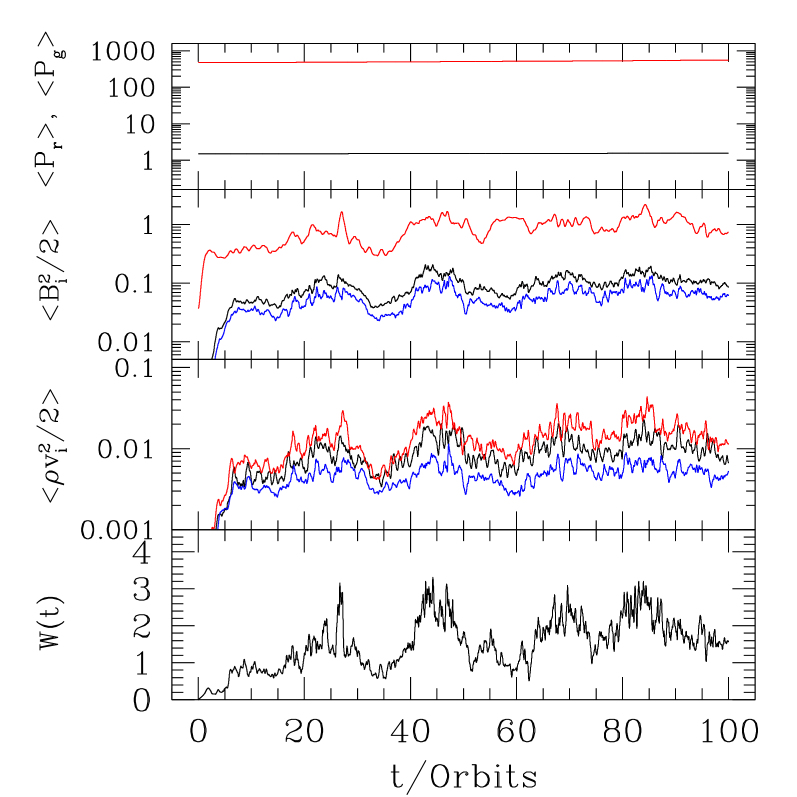
Figure 4.— The same as Figure 1 but for simulation YFR3Res with net toroidal flux.

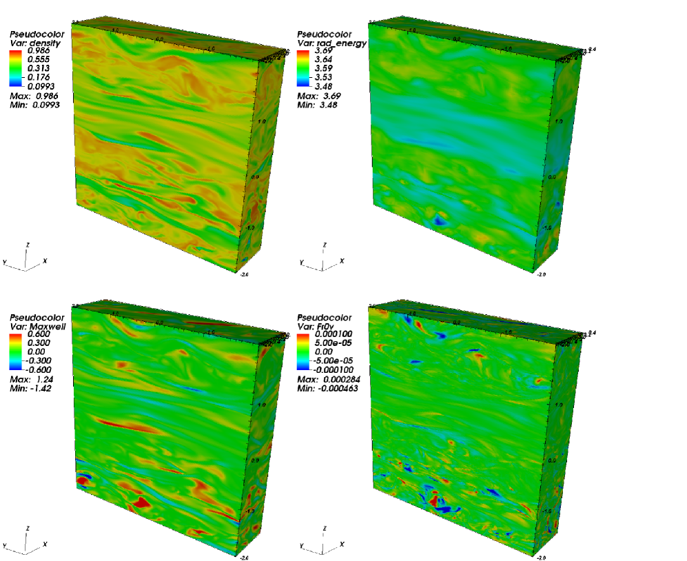
Figure 5.— Snapshots of simulation YFR1Res at time $25.1$ orbits. From left to right, top to bottom, are density $\rho$, radiation energy density $E_{r}$, Maxwell stress $-B_{x}B_{y}$ and co-moving flux projected along the direction of perturbed velocity $({\mbox{\boldmath$F$}}_{r,0}\cdot\delta{\mbox{\boldmath$v$}})/|\delta{\mbox{\boldmath$v$}}|$.

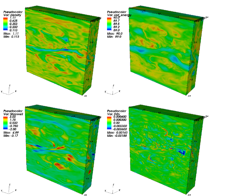
Figure 6.— The same as Figure 5 but for simulation YFR3Res at time $72.0$ orbits.

3.2.2 Time Evolution

Temporal evolution of radiation and gas pressure, three components magnetic and kinetic energy densities as well as the total work done on the wall of the simulation box per unit time for simulation YFR3Res are shown in Figure 4. Because the initial radiation energy density is so large, within $100$ orbits, the total energy only increases $16.7\%$ due to the work done on the wall of the simulation box. Similar to case with net vertical flux, kinetic and magnetic energy densities saturate quickly after initial transient and fluctuate, although the total energy density never reaches an equilibrium value.

In Figure 5, we show snapshots of $\rho$, $E_{r}$, $-B_{x}B_{y}$ and $({\mbox{\boldmath$F$}}_{r,0}\cdot\delta{\mbox{\boldmath$v$}})/|\delta{\mbox{\boldmath$v$}}|$ for simulation YFR1Res at time $25.1$ orbits. Here $\delta{\mbox{\boldmath$v$}}$ is the perturbed velocity with the background shear subtracted. The same quantities for simulation YFR3Res at time $72.0$ orbits are shown in Figure 6. Similar to the simulations in Table 1, YFR1Res and YFR3Res are also very compressible. The ratio between the maximum and minimum densities is $\sim 10$. Most of the Maxwell stress is located in regions where the density variations are large, with the largest values in the low density regions. The radiation energy density has a similar distribution as density because $E_{r}$ is also compressed when $\rho$ is compressed. Therefore the co-moving flux ${\mbox{\boldmath$F$}}_{r,0}$ is also large when the density gradient is large. Radiation energy density $E_{r}$ in simulation YFR3Res is $81$ times the value in simulations YFR1Res while the co-moving flux is almost a factor of $8$ larger in simulation YFR3Res than YFR1Res. This means that the radiation force on the fluid in YFR3Res is also about $8$ times larger than the radiation force in YFR1Res. The sign of the quantity $({\mbox{\boldmath$F$}}_{r,0}\cdot\delta{\mbox{\boldmath$v$}})/|\delta{\mbox{\boldmath$v$}}|$ represents the relative direction between the co-moving flux and the velocity field. When it is positive, photons accelerate the fluid during expansion while it is negative, photons decelerate the fluid during compression. The net effect is that part of the kinetic energy is converted to gas internal and radiation energy, resulting in damping due to radiation drag (Agol & Krolik, 1998). The fact that co-moving flux in simulation YFR3Res is about $8$ times larger than the co-moving flux in simulation YFR1Res, implies that the radiation damping effect in YFR3Res will also be much larger than this effect in YFR1Res. The consequences of the radiation drag effect will be examined in more detail in the following sections.

Table 3Parameters for simulations with net toroidal flux

Label	$P_{g}$	$P_{r}$	$N$/$L_{0}$
YFNR	6.37	—	32
YFR1	0.50	5.87	32
YFR2	1.00	93.92	32
YFR3	1.50	475.47	32
YFR1Res	0.50	5.87	64
YFR2Res	1.00	93.92	64
YFR3Res	1.50	475.47	64

3.2.3 Statistical Properties

Averaged properties between $10$ and $100$ orbits for these simulations are shown in Table 4. By comparing YFR1, YFR2, YFR3 and YFR1Res, YFR2Res and YFR3Res, we see that when the initial temperature is $T_{0}$, the simulation with $32$ cells per $L_{0}$ is already converged, while for the simulations with initial temperatures $2T_{0}$ and $3T_{0}$, this is not the case. To check the convergence of the high temperature runs, we carry out another simulation with $128$ grids per $L_{0}$ for initial temperature $3T_{0}$. We only run this high resolution module for $40$ orbits. Averaging over the last $20$ orbits, $\,\langle\langle-B_{x}B_{y}\,\rangle\rangle=0.220$, $\,\langle\langle\rho v_{x}\delta v_{y}\,\rangle\rangle=0.00780$ and $\alpha_{\text{mag}}=0.258$. Comparing this run and simulations YFR3 and YFR3Res, we find that the differences between $64$ cells and $128$ cells per $L_{0}$ are much smaller than the differences between $32$ cells and $64$ cells per $L_{0}$. For example, the Maxwell and Reynolds stress only change within the statistical fluctuations when we go from $64$ to $128$ cells per $L_{0}$. Thus, we infer that the high temperature runs with $64$ cells per $L_{0}$ are approaching convergence. The analysis below will focus on the four simulations YFNR, YFR1Res, YFR2Res and YFR3Res.

Table 4Temporal and Spatial Averaged Properties of Simulations with Net Azimuthal flux

Label	$\,\langle\langle-B_{x}B_{y}\,\rangle\rangle$	$\,\langle\langle\rho v_{x}\delta v_{y}\,\rangle\rangle$	$\,\langle\langle B^{2}/2\,\rangle\rangle$	$\,\langle\langle B_{x}^{2}/2\,\rangle\rangle$	$\alpha_{\text{stress}}$
YFNR	0.0330	0.00730	0.123	0.0122	4.52
YFR1	0.0469	0.00580	0.236	0.0169	8.09
YFR2	0.0737	0.00290	0.322	0.0237	25.4
YFR3	0.0547	$5.27\times 10^{-4}$	0.261	0.0129	104
YFR1Res	0.0425	0.00670	0.199	0.0175	6.34
YFR2Res	0.125	0.00660	0.666	0.0462	18.9
YFR3Res	0.249	0.00570	1.01	0.0913	43.7
Label	$\,\langle\langle B_{y}^{2}/2\,\rangle\rangle$	$\,\langle\langle B_{z}^{2}/2\,\rangle\rangle$	$\,\langle\langle T/T_{0}\,\rangle\rangle$	$\alpha_{\text{mag}}$	$\alpha$
YFNR	0.107	0.00410	3.03	0.267	0.00632
YFR1	0.210	0.00920	1.21	0.199	0.00826
YFR2	0.281	0.0175	2.01	0.160	0.000806
YFR3	0.236	0.0117	3.02	0.210	0.000116
YFR1Res	0.174	0.00790	1.20	0.214	0.00772
YFR2Res	0.592	0.0279	2.09	0.188	0.00140
YFR3Res	0.861	0.0561	3.05	0.247	0.000534

3.2.4 Change of Maxwell stress with total pressure

All the simulations done in this paper have fixed vertical box size and thus we cannot study the increase of Maxwell stress due to the increase of disk scale height, which we expect to be the primary source of connection between stress and pressure. This will be studied in future work. However, as Figure 7 shows, even with fixed box size, the Maxwell stress is increased with increasing total pressure. Compared with simulation YFR1Res with temperature $T=T_{0}$, initial total pressure is increased by a factor of $15$ when temperature $T=2T_{0}$ (run YFR2) and a factor of $75$ when temperature $T=3T_{0}$ (run YFR3). However, total stress is only increased by a factor of 2.67 from simulation YFR1Res to YFR2Res, and a factor of $5.18$ from simulation YFR1Res to YFR3Res.

To identify the cause of increase in Maxwell stress as total pressure increases, we have studied the magnitudes of the radiation source terms in detail. In equation (3), the terms that are responsible for the radiation drag effect are the radiation momentum source term ${\bf S_{r}}({\mbox{\boldmath$P$}})$ and the velocity dependent radiation work terms in the radiation energy source term $S_{r}(E)$. The amplitude of these source terms for simulations YFR1Res, YFR2Res and YFR3Res can be measured directly from the simulation data. We first calculate the spatial and temporal averaged radiation momentum source term $S_{p}\equiv\,\langle\langle{\mathbb{P}}(\sigma_{aF}+\sigma_{sF})|{\mbox{\boldmath$F$}}_{r,0}|\,\rangle\rangle$. The temporal average is taken over $10$ and $100$ orbits to avoid the effect of initial transients. For YFR1Res, YFR2Res and YFR3Res, in units of $\rho_{0}a_{0}\Omega$, $S_{p}$ are $1.01$, $3.90$ and $6.38$ respectively. As expected, the radiation momentum source term is increased when temperature and thus radiation pressure is increased. Second, we calculate $t_{r}=\,\langle\langle E_{k}\,\rangle\rangle/\,\langle\langle W_{r}\,\rangle\rangle$, the averaged ratio between the kinetic energy $E_{k}$ and the radiation work term $W_{r}\equiv-{\mathbb{P}}(\sigma_{aF}-\sigma_{sF}){\mbox{\boldmath$v$}}\cdot{\mbox{\boldmath$F$}}_{r,0}$. This is the time scale to change the kinetic energy due to the work done by the radiation force. Here $E_{k}$ does not include the kinetic energy due to background Keplerian motion. For simulations YFR1Res, YFR2Res and YFR3Res, in our time unit $\Omega^{-1}$, $t_{r}$ is $-5.70$, $-3.33$ and $-3.20$ respectively. Here $t_{r}$ is negative, which means that the co-moving flux prefers to point to the opposite direction of fluid motion and decelerates it on average. The time scale is shorter for simulations YFR2Res and YFR3Res, only about half an orbital period. To make sure that the momentum source term ${\bf S_{r}}({\mbox{\boldmath$P$}})$ is the key to the increase the Maxwell stress, we have also carried out another test in which we remove the momentum source term ${\bf S_{r}}({\mbox{\boldmath$P$}})$ and the radiation work terms in the radiation energy source terms. We use the same setup as simulation YFR3Res. We find almost the same Maxwell stress and Reynolds stress as simulation YFR1Res and YFNR. Therefore, if there is no damping of fluid motion by the photons, we find the same saturation level as in the pure gas pressure case. This is strong evidence that it is radiation damping that is responsible for the increase of the Maxwell stress.

The importance of the radiation drag effect can also be quantified by the photon bulk viscosity (e.g., Castor, 2004). In our units, the radiation bulk viscosity is (equation 6.80 of Castor 2004)

$$\xi_{r}=4{\mathbb{P}}E_{r}/\left(9\sigma_{t}{\mathbb{C}}\right),$$ (17)

where $\sigma_{t}=\sigma_{aF}+\sigma_{sF}$. A Reynolds number can be defined based on the radiation bulk viscosity, and the typical velocity, length scale and density (isothermal sound speed $c_{s}$, scale height $c_{s}/\Omega$ and fiducial density $\rho_{0}$ respectively), that is

$$R_{e}=\rho_{0}c^{2}_{s}/\left(\Omega\xi_{r}\right).$$ (18)

For simulations YFR1Res, YFR2Res and YFR3Res, the Reynolds numbers are $1.91\times 10^{5}$, $1.18\times 10^{4}$ and $2.33\times 10^{3}$ respectively. For simulation ZFRS, this number is $5.71\times 10^{4}$.

Our simulations also include grid scale dissipation set by numerical viscosity and resistivity. In order for the photons to control the magnetic dissipation rate, the Prandtl number defined by the ratio between radiation bulk viscosity and the numerical resistivity needs to be larger than $1$. Numerical resistivity is likely problem dependent. Simon et al. (2009) quantifies the effective magnetic Reynolds number based on numerical resistivity in Athena to be around $5\times 10^{3}-1\times 10^{4}$. Simon & Hawley (2009) also find that when the Reynolds number for the explicit (shear) viscosity is smaller than $6400$, the Maxwell stress begins to show a significant increase. Therefore we suggest that radiation pressure in simulations YFR2Res and YFR3Res is large enough to change the Maxwell stress significantly while in simulations YFR1Res and ZFRS, it is not.

A similar result for the unstratified disk model was also reported for the pure gas pressure case by Sano et al. (2004). They studied the saturation level of MRI for a wide range of gas pressure and found that Maxwell stress has a weak dependence on the gas pressure. For the zero net flux case, they found $\,\langle\langle-B_{x}B_{y}\,\rangle\rangle\propto P^{1/4}$ while for the net vertical flux case, they found $\,\langle\langle-B_{x}B_{y}\,\rangle\rangle\propto P^{1/6}$. There is no definite explanation for the weak dependence of Maxwell stress on the gas pressure. They argue that higher gas pressure can reduce the magnetic reconnection rate and thus reduce the dissipation rate of magnetic energy, resulting in a higher Maxwell stress in the saturation state. More recently, studies with explicit viscosity and resistivity (e.g., Lesur & Longaretti, 2007; Fromang & Papaloizou, 2007; Simon & Hawley, 2009; Simon et al., 2009) found that at moderate Reynolds number $Re$, the Maxwell stress from the saturation states of MRI turbulence increases with the magnetic Prandtl number $Pm=\nu/\eta$, which is the ratio between microscopic viscosity and resistivity. Following Balbus & Hawley (1998), Simon & Hawley (2009) argues that viscosity can prevent motion that would bring field together on small scales and therefore reduce the magnetic reconnection rate. The increase of Maxwell stress with radiation pressure found here, may be due to a similar mechanism, except that the change of effective Prandtl number is caused by the damping of radiation field on the compressible motions in the fluid, rather than explicit viscosity.

3.2.5 The ratio between Maxwell stress and Reynolds stress

The change in the effective Prandtl number due to radiation drag also seems to affect the ratio of the Maxwell to Reynolds stress. In Figure 7, when the Maxwell stress is increased with increasing radiation pressure, the Reynolds stress stays at almost the same level. Therefore, the ratio between Maxwell stress and Reynolds stress is increased when radiation pressure is increased. As calculated in Table 3, this ratio is $6.34$ for YFR1Res and it increases to $18.9$ and $43.7$ for YFR2 and YFR3 respectively. As a comparison, the ratio is only $4.52$ for the simulation YFNR without radiation. This ratio reported in most MRI simulations with or without radiation is also around $4-5$ (e.g., Hawley et al., 1995; Turner et al., 2003; Sano et al., 2004; Davis et al., 2010). However, when Simon & Hawley (2009) includes explicit viscosity in their MRI simulations, they finds that the ratio between Maxwell stress and Reynolds stress increases when the stress and viscosity is increased, although the change of this ratio is not as large as what we find here.

In the test run in which we remove the radiation momentum source term described in the last section, we find the usual ratio between Maxwell stress and Reynolds stress as in the pure gas pressure case. We also notice that for all the simulations listed in Table 1, where we find the radiation damping is not important, the ratio between Maxwell stress and Reynolds stress is also normal. This ratio is only significantly increased for those simulations listed in Table 3, where the Maxwell stress is much larger than what the values would be if the radiation pressure is replaced with the same amount of gas pressure. Those results suggest that the change of the ratio between Maxwell stress and Reynolds stress is due to the same physical mechanism responsible for the increase of Maxwell stress discussed in the last section, which is the damping of the compressive motions due to radiation drag. We have also checked that this result is independent of field geometry. When we use net vertical magnetic flux, we get the same result.

We also notice that $\alpha_{\text{mag}}$ for those simulations listed in Table 3 is systematically smaller than $\alpha_{\text{mag}}$ from non-radiative MRI simulations. It is also smaller than $\alpha_{\text{mag}}$ for the simulations listed in Table 1, which have net vertical magnetic flux. For simulations YFR1Res, YFR2Res and YFR3Res, $\alpha_{\text{mag}}$ varies from $0.188$ to $0.247$ with the average value to be $0.21$. For simulations ZFRS, ZFRL, ZFNRS, ZFNRL and ZFRS64, $\alpha_{\text{mag}}$ is always between 0.4 and 0.5, which is also the usual value reported by most non-radiative MRI simulations (e.g., Hawley et al., 2011). A smaller $\alpha_{\text{mag}}$ is also found from stratified simulations of radiation dominated accretion disk done with ZEUS (Krolik et al., 2012, private communication).

3.2.6 Radiative Viscosity

In the radiation dominated flow around the black holes, it has been argued that radiative viscosity can be important to transfer the angular momentum, which can even be the dominant mechanism for spherical accretion flows (e.g., Loeb & Laor, 1992). Radiative viscosity will only be important when the radiation energy density is significant. Here, we can compare the viscous stress due to radiation with the Maxwell and Reynolds stress for simulation YFR3Res, which has the largest radiative viscosity in our simulations.

In principle, the off-diagonal component of the co-moving radiation pressure in the $x-y$ plane, which is responsible for the transfer of angular momentum, comes from two parts in our formula. The first part is the off-diagonal component of the Eddington tensor in the Eulerian frame. We have calculated the VET for simulation YFR3Res with the short-characteristic module, and find that the off-diagonal components of the VET is smaller than $10^{-8}$. Thus it can be neglected. The second part is the radiative shear viscosity, the formula of which is (e.g., Castor, 2004)

$$P_{r,xy}=-\frac{4{\mathbb{P}}E_{r}}{15\sigma_{t}{\mathbb{C}}}\left(\frac{\partial v_{x}}{\partial y}+\frac{\partial v_{y}}{\partial x}\right).$$ (19)

This is caused by the velocity dependent radiation momentum source terms. For simulation YFR3Res, the spatially and timely averaged value is $\,\langle\langle P_{r,xy}\,\rangle\rangle=4.13\times 10^{-4}$ in our fiducial units. The radiative viscosity is dominated by the background shearing. Therefore, even for simulation YFR3Res, the off-diagonal component of the co-moving radiation pressure is only $1.66\times 10^{-3}$ of the Maxwell stress and $7.2\%$ of the Reynolds stress.

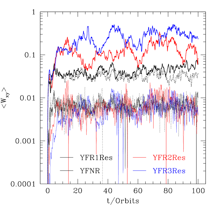
Figure 7.— History of the spatially averaged Maxwell and Reynolds stress for simulations with net azimuthal flux. Maxwell stress is plotted as the upper thick lines while the Reynolds stress is plotted as the lower thin lines. Parameters of all the simulations shown in this figure are listed in Table 3. YFR1Res, YFR2Res and YFR3Res differ in the initial ratio between radiation pressure and gas pressure, which increases by a factor of $27$ from YFR1Res to YFR3Res. YFNR is a comparison simulation without radiation field but the same total pressure as YFR1Res.

4. Discussion and Conclusion

With our recently developed Godunov radiation MHD code, we have confirmed the results of Turner et al. (2003) for unstratified optically thick mid-plane of a radiation dominated accretion disk. In particular, we find when the photon diffusion length per orbit is larger than the most unstable MRI wavelength, the MRI turbulence becomes very compressible. Furthermore, we extend the fiducial simulations of Turner et al. (2003) by increasing the radial size by a factor of $4$, which allows more radial modes to exist in the simulation box. The saturation level of the MRI from the larger simulation domains is very similar to what we find in the fiducial runs. Recurrent channel solutions observed in small box simulations do not exist when radial size is increased. This is consistent with what Bodo et al. (2008) found without radiation. In this sense, radiation pressure plays the same role as gas pressure in the optically thick regime.

When the radiation energy density is increased to a non-negligible fraction ($\gtrsim 1\%$) of fluid rest mass energy, we find that Maxwell stress is increased with increasing radiation pressure. At the same time, Reynolds stress seems to be independent of radiation pressure. Therefore, the ratio between Maxwell and Reynolds stress is increased with increasing radiation pressure. We suggest that this is due to the damping effect of radiation drag which introduces an effective bulk viscosity $\xi_{r}$. To quantify the importance of the radiation damping effect, we have calculated the Reynolds number based on $\xi_{r}$ (equation 17) and find values of $\sim 2.33\times 10^{3}$ for the simulation with the largest radiation pressure. This number depends on ${\mathbb{P}}E_{r}/{\mathbb{C}}$ in our units for a fixed opacity, which is actually the momentum of the photons. This can explain why we do not see the change of Maxwell stress as well as the ratio between Maxwell and Reynolds stress compared to the pure gas pressure case for the simulations listed in Table 1. Although the ratio between radiation pressure and gas pressure is $125$ for the simulations listed in Table 1, ${\mathbb{P}}E_{r}/{\mathbb{C}}$ is only $7.7\%$. While for the simulations listed in Table 3, ${\mathbb{P}}E_{r}/{\mathbb{C}}$ is $0.035$, $0.567$ and $2.87$ for $T=T_{0},2T_{0},3T_{0}$ respectively.

Because there is no cooling in the unstratified simulations, the disk is continuously heated up due to the dissipation of MRI. However, as the histories of these simulations show (Figure 2 and Figure 7), the secular build-up of energy in these simulations does not affect the diagnostics we are interested, such as Maxwell stress and Reynolds stress. This is not surprise, because the effects discussed this in paper requires $T$ to increase by a factor of $2$ and $3$, while during the $100$ orbits of YFR1, YFR2Res and YFR3Res, $T$ is only increased by $40\%$, $9\%$ and $4\%$ respectively.

Even when radiation energy density reaches $1\%$ of the fluid rest mass energy density as in simulation YFR3Res, we find that the off-diagonal component of the co-moving radiation pressure is much smaller than the Maxwell and Reynolds stress. This confirms that transfer of angular momentum by radiative viscosity is not the dominant mechanism when the turbulence due to MRI exists.

We perform two sets of simulation with both high ($N/L_{0}=64$) and low ($N/L_{0}=32$) resolution. We find consistent (statistically equivalent) estimates for turbulent properties, such as the stress, which suggests these simulations are converged. Since we do not include explicit resistivity, our results may have been sensitive to the effective amount of “numerical resistivity”, which is strongly resolution dependent (e.g., Simon et al., 2009). Our result implies that effective resistivity is sufficiently small that turbulent properties are set primarily by dynamics at larger scales and not strongly impacted by the precise properties of grid scale dissipation.

In all the simulations, we have fixed the the Eddington tensor to be $1/3\delta_{ij}$ in the Eulerian frame. Since our simulations are approximating the mid-plane of an optically thick accretion disk, the assumption of isotropy is well justified, but it is generally expected that the radiation field will be nearly isotropic in the co-moving frame. As the difference between co-moving radiation pressure and Eulerian radiation pressure in our units is ${\mbox{\boldmath$v$}}\cdot{\mbox{\boldmath$F$}}_{r,0}/{\mathbb{C}}$ (e.g., Mihalas & Mihalas, 1984), the difference between Eulerian Eddington tensor and co-moving Eddington tensor will be ${\mbox{\boldmath$v$}}\cdot{\mbox{\boldmath$F$}}_{r,0}/({\mathbb{C}}E_{r})$, which we confirm is less than $10^{-4}$ for all the simulations presented here. Therefore, this assumption should not appreciably impact our results. A test with Eddington tensor to be $1/3\delta_{ij}$ in the co-moving frame does confirm this conclusion.

We have also calculated VET with the short characteristic module described in Davis et al. (2012) for the simulations shown in Table 1. For the unstratified shearing box disk models, there is no preferred direction for the specific intensity because periodic or shearing periodic boundary conditions are applied for all three directions. Furthermore, photon mean free paths for all the simulations are smaller than the cell size. Therefore, VET returned by the short characteristic module only differs from $1/3{{\sf\boldmath I}}$ by $10^{-4}$, when $24$ angles are used. This confirms that Eddington approximation is valid for the unstratified disk models, which are designed to study the optically thick mid-plane of accretion disks.

The increase of Maxwell stress with increasing radiation pressure and the change of $\alpha_{\text{stress}}$ have important implications. This study confirms that the damping effect of large radiation pressure will not decrease the total stress. Instead, the total stress is actually increased slowly with total pressure when radiation energy density is significant.

These results also confirm the important role radiation viscosity plays as a source of microscopic dissipation in radiation dominated regions of accretion flows. Although radiation viscosity always plays a subdominant role to Maxwell and Reynolds stresses in angular momentum transport, it will generally exceed the standard plasma viscosity. In cgs units, Equation (17) corresponds to a kinematic viscosity with

$$\nu_{r}\simeq\frac{4a_{r}T^{4}}{9\kappa_{\rm T}\rho^{2}c}=3.4\times 10^{-25}\frac{T^{4}}{\rho^{2}}\ {\rm cm}^{2}\ {\rm s}^{-1}.$$ (20)

This can be compared with Equation (2) of Balbus & Henri (2008), which gives an estimate of the plasma viscosity $\nu_{p}\propto T^{5/2}/\rho$. In the radiation dominated regimes of accretion flows, $\nu_{r}>\nu_{p}$ when $T\lesssim 10^{9}$ K and it is often the case that $\nu_{r}\gg\nu_{p}$. It is still true for the hottest radiation dominated flows ($T\gtrsim 10^{9}$ K) when $\rho<4.74\times 10^{4}\left(T/10^{9}\ \text{K}\right)^{3/2}$ g cm^-3. So radiation is the dominant viscosity associated with microscopic dissipation. This makes radiation dominated accretion disk one of the few regimes where the physically relevant value of the viscosity can be numerically resolved with current computing resources. The ratio $\nu_{r}/\nu_{p}$ is larger for the accretion disks around supermassive black holes than solar mass black holes, which may lead to different properties of the accretion flows for systems in the two different scales if the radiation viscosity becomes important.

Despite the dominance of radiative viscosity, it is generally true that plasma resistivity dominates over radiative resistivity, even in radiation dominated accretion flows (Agol & Krolik, 1998). Therefore, Equation (1) of Balbus & Henri (2008) still gives the relevant magnetic resistivity $\eta$. Since this quantity is generally very small compared with $\nu_{r}$, the corresponding magnetic Prandtl number ${\rm Pm}=\nu_{r}/\eta\gg 1$ in radiation dominated flows. This conclusion is interesting in light of speculation that Pm may be the primary parameter that controls angular momentum transport by the MRI (Fromang et al., 2007). A large Pm would place radiation dominated accretion flows firmly in the efficient angular momentum regime if this supposition is correct.

In all the unstratified disk simulations, the total energy can never reach an equilibrium value because there is no cooling in these simulations. However, the Maxwell and Reynolds stress saturate quickly after an initial transient. Even when total pressure is increased by a factor of $2$, the stress does not show any systematic trend of change within the first $100$ orbits of the simulations. This is because the saturation level in the unstratified disk models is limited by the box size. As found by Hawley et al. (1995), Maxwell stress in the saturated state increases linearly with box size in their unstratified disk models. Therefore, the unstratified disk models cannot be used to check the assumed relation between stress and pressure in the $\alpha$ disk model, which requires the change of disk scale height to connect them. The fact that the effective $\alpha$ value decreases when total pressure increases for these unstratified simulations is an artifact of the closed-box assumption, which should not be interpreted literally. When the total pressure increases, the disk scale height will also be increased, which gives more space for the turbulence to develop. The weak dependence of Maxwell stress on the radiation pressure due to the mechanism suggested here is probably not the dominant process in real accretion disks. More realistic stratified disk models will be studied in the future. Nevertheless, the phenomenon we find here is also likely to operate in the mid-plane of the accretion disk near the Eddington limit. In the future, we will perform more realistic stratified disk models that will be better suited for addressing these questions.

Appendix A Improvements to the Numerical Algorithm

The code used in this paper is based on the algorithm described in JSD12, with several important improvements. Based on our tests, those improvements are necessary to reduce numerical diffusion in the optically thick regime while leave the optically thin regime unaffected.

A.1. Effective photon propagation speed

The first change is the HLLE Riemann solver for the radiation subsystem (the last two lines of equation 3). As described in §3.3.2 of JSD12, the HLLE Riemann solver is used to calculate the flux for the radiation subsystem. In JSD12, the characteristic speed along each direction is always chosen to be $\sqrt{f}{\mathbb{C}}$, where $f$ is the component of the Eddington tensor along that direction, following Sekora & Stone (2010) (see their equation 46). However, as discussed by Audit et al. (2002), when the optical depth per cell is larger than one, the numerical diffusive flux due to the HLLE Riemann solver can be much larger than the physical radiative flux, which can cause unphysical solutions. This issue does not appear in the tests done by Sekora & Stone (2010) because they only consider pure absorption opacity. In the optically thick regime, the evolution of radiation energy density is dominated by the source term ${\mathbb{C}}\sigma_{a}(T^{4}-E_{r})$ because the thermalization time is usually very short. However, for scattering opacity dominated cases, the energy source term is very small and the radiation flux term ${\mbox{\boldmath$\nabla$}}\cdot{\mbox{\boldmath$F$}}_{r}$ controls the change of $E_{r}$. If the numerical diffusive flux is much larger than the physical radiation flux, the photon diffusion time will be significantly underestimated.

Audit et al. (2002) fixes this issue by changing the term ${\mbox{\boldmath$\nabla$}}\cdot{\sf P_{r}}$ in their dimensionless units (see their equation 46). This is equivalent to reducing the characteristic speed of the radiation modes in the optical thick regime. To find the appropriate effective speed for different frequency mean opacity $\sigma_{t}\equiv\sigma_{aF}+\sigma_{sF}$, we carry out a linear analysis for the following 1D equations

$$\frac{\partial E_{r}}{\partial t}+\mathbb{C}\frac{\partial F_{r}}{\partial x} = 0,$$

$$\frac{\partial F_{r}}{\partial t}+f\mathbb{C}\frac{\partial E_{r}}{\partial x} = -\mathbb{C}\sigma_{t}F_{r}.$$ (A1)

The background state is a static medium with a uniform radiation field. For mode with wavenumber $k$, the propagation speed is

$$C_{eff}=\sqrt{f}{\mathbb{C}}\sqrt{1-\frac{\sigma_{t}^{2}}{4fk^{2}}}.$$ (A2)

In the optically thin limit when $\sigma_{t}\rightarrow 0$, the effective speed of light $C_{eff}$ approaches $\sqrt{f}{\mathbb{C}}$. In the optically thick limit, $C_{eff}$ is much smaller than $\sqrt{f}{\mathbb{C}}$. Especially, for modes with $\sigma_{t}^{2}/(4fk^{2})>1$, the propagation speed of the photons is zero, which means photons only diffuse through the medium instead of free-streaming. Because we solve the radiation subsystem implicitly, the distance that photons can travel for a give time step $dt$ is not limited by the size of each cell. The lower limit for the wave number $k$ should be $1/(\Delta t{\mathbb{C}})$. However, this value is usually too restrictive and makes the resulting matrix from the implicit radiation subsystem very hard to invert. Instead, another characteristic length is the size of each cell. Based on our tests, we find that if we calculate the effective propagation speed with a wave length of ten cells, the numerical diffusion is small enough not to affect the solution. If the size of each cell is $\Delta l$, to connect the optically thin and optically thick regimes smoothly, the effective propagation speed we use is

$$C_{eff}^{\star} = {\mathbb{C}}\sqrt{\frac{f}{\tau}\left[1-\exp{\left(-\tau\right)}\right]},$$

$$\tau \equiv (10\Delta l\times\sigma_{t})^{2}/\left(2f\right).$$ (A3)

In the optically thin limit, the effective speed is reduced to equation A2 with wavenumber $k=1/(10\Delta l)$. In optically thick limit, the effective speed $C_{eff}\propto 1/(\Delta l\times\sigma_{t})$. The purpose of using $C_{eff}^{\star}$ instead of ${\mathbb{C}}$ is to reduce the numerical diffusion so that we can capture the physical radiation flux, which is small in the diffusion regime. As long as physical radiation flux is dominant over the numerical flux in all regimes, the solution is more accurate. Tests presented below do confirm this.

A.2. Advection Flux

In the optically thick regime, the diffusive flux is very small, and the change of radiation energy density can be dominated by the advection flux. We find that the first order treatment for the radiation subsystem described in JSD12 is too diffusive for the advection flux. In order to improve the accuracy, we separate the advection flux from the diffusive flux and treat the advection flux explicitly with second order accuracy.

For a given velocity $v$, the change of $E_{r}$ due to the advection flux is

$$\frac{\partial E_{r}}{\partial t}+{\mbox{\boldmath$\nabla$}}\cdot({\mbox{\boldmath$v$}}E_{r})=0.$$ (A4)

Because the radiation subsystem is separated from the MHD part, the flow velocity $v$ is taken to be constant during this step. We first calculate the flow velocity at the edge of each cell $V_{i+1/2}$ by taking the average of cell centered velocities in the two neighboring cells. We use the van Leer slope (equation 48 and 49 of Stone & Norman 1992) to interpolate $E_{r}$ from cell centers to cell edges $E_{r,i+1/2}$. Then the advection flux on each cell edge $\mathcal{F}_{i+1/2}$ is just $\mathcal{F}_{i+1/2}=V_{i+1/2}E_{r,i+1/2}$.

A.3. The New Implicit Backward-Euler Step

In order to incorporate the above two improvements into our implicit Backward Euler step, we first rewrite the radiation subsystem into the following form

$$\frac{\partial E_{r}}{\partial t}+\mathbb{C}{\mbox{\boldmath$\nabla$}}\cdot\left({\mbox{\boldmath$F$}}_{r}-\frac{{\mbox{\boldmath$v$}}E_{r}+{\mbox{\boldmath$v$}}\cdot{\sf P}_{r}}{{\mathbb{C}}}\right)+{\mbox{\boldmath$\nabla$}}\cdot\left({\mbox{\boldmath$v$}}\cdot{\sf P}_{r}\right) = -{\mbox{\boldmath$\nabla$}}\cdot\left({\mbox{\boldmath$v$}}E_{r}\right)+\mathbb{C}S_{r}(E),$$

$$\frac{\partial{\mbox{\boldmath$F$}}_{r}}{\partial t}+\mathbb{C}{\mbox{\boldmath$\nabla$}}\cdot{\sf P}_{r} = \mathbb{C}{\bf S_{r}}({\mbox{\boldmath$P$}}).$$ (A5)

Notice that ${\mbox{\boldmath$F$}}_{r,0}={\mbox{\boldmath$F$}}_{r}-\left({\mbox{\boldmath$v$}}E_{r}+{\mbox{\boldmath$v$}}\cdot{\sf P}_{r}\right)/{\mathbb{C}}$ is actually the co-moving flux. In this way, the advection part ${\mbox{\boldmath$\nabla$}}\cdot\left({\mbox{\boldmath$v$}}\cdot{\sf P}_{r}+{\mbox{\boldmath$v$}}E_{r}\right)$ is separated from the flux in the co-moving frame ${\mbox{\boldmath$\nabla$}}\cdot{\mbox{\boldmath$F$}}_{r,0}$. The advection part ${\mbox{\boldmath$\nabla$}}\cdot\left({\mbox{\boldmath$v$}}\cdot{\sf P}_{r}+{\mbox{\boldmath$v$}}E_{r}\right)$ is the advective radiation enthalpy (e.g., Castor, 2004). Only the ${\mbox{\boldmath$\nabla$}}\cdot\left({\mbox{\boldmath$v$}}E_{r}\right)$ part is treated as described in §A.2, while the ${\mbox{\boldmath$\nabla$}}\cdot\left({\mbox{\boldmath$v$}}\cdot{\sf P}_{r}\right)$ part is solved implicitly with the source terms.

First, with the velocity field $v$ and $E_{r}^{n}$ at time step $n$, we calculate the advection flux along each direction $\mathcal{F}_{i+1/2,j,k}$, $\mathcal{F}_{i,j+1/2,k}$, $\mathcal{F}_{i,j,k+1/2}$ as described in §A.2 for each cell. Then we calculate the implicit HLLE fluxes ${\sf\mathbb{F}^{\text{HLLE}}}$ according to equation (39) of Sekora & Stone (2010) for the following equation

$$\frac{\partial E_{r}}{\partial t}+\mathbb{C}{\mbox{\boldmath$\nabla$}}\cdot\left({\mbox{\boldmath$F$}}_{r}-\frac{{\mbox{\boldmath$v$}}E_{r}+{\mbox{\boldmath$v$}}\cdot{\sf P}_{r}}{{\mathbb{C}}}\right) = 0,$$

$$\frac{\partial{\mbox{\boldmath$F$}}_{r}}{\partial t}+\mathbb{C}{\mbox{\boldmath$\nabla$}}\cdot{\sf P}_{r} = 0.$$ (A6)

The following changes are made during the calculation of the HLLE fluxes. The maximum and minimum wave speeds we actually use are $C_{eff}^{\star}$ and $-C_{eff}^{\star}$ respectively, where $C_{eff}^{\star}$ is calculated according to equation A3. In order to make the implicit matrix easier to invert for the cases with sharp opacity jump, the opacity $\sigma_{t}$ we use to calculate $C_{eff}^{\star}$ on the cell edges is the average opacity of two neighboring cells. The term ${\mbox{\boldmath$\nabla$}}\cdot\left({\mbox{\boldmath$v$}}\cdot{\sf P}_{r}\right)$ is calculated implicitly as

$${\mbox{\boldmath$\nabla$}}\cdot\left({\mbox{\boldmath$v$}}\cdot{\sf P}_{r}\right)(i,j,k) = \left[{\mbox{\boldmath$v$}}\cdot{\sf P_{r}^{n+1}}(i+1)-{\mbox{\boldmath$v$}}\cdot{\sf P_{r}^{n+1}}(i-1)\right]/(2\Delta x)$$ (A7)

$$+ \left[{\mbox{\boldmath$v$}}\cdot{\sf P_{r}^{n+1}}(j+1)-{\mbox{\boldmath$v$}}\cdot{\sf P_{r}^{n+1}}(j-1)\right]/(2\Delta y)$$

$$+ \left[{\mbox{\boldmath$v$}}\cdot{\sf P_{r}^{n+1}}(k+1)-{\mbox{\boldmath$v$}}\cdot{\sf P_{r}^{n+1}}(k-1)\right]/(2\Delta z).$$

Then radiation energy density $E_{r}$ is updated as

$$E_{r,i,j,k}^{n+1} = E_{r,i,j,k}^{n}-\frac{\Delta t}{\Delta x}\left[{\bf F}^{HLLE}_{i+1/2,j,k}-{\bf F}^{HLLE}_{i-1/2,j,k}\right]-\frac{\Delta t}{\Delta y}\left[{\bf F}^{HLLE}_{i,j+1/2,k}-{\bf F}^{HLLE}_{i,j-1/2,k}\right]$$ (A8)

$$- \frac{\Delta t}{\Delta z}\left[{\bf F}^{HLLE}_{i,j,k+1/2}-{\bf F}^{HLLE}_{i,j,k-1/2}\right]-\frac{\Delta t}{\Delta x}\left[\mathcal{F}_{i+1/2,j,k}-\mathcal{F}_{i-1/2,j,k}\right]$$

$$- \frac{\Delta t}{\Delta y}\left[\mathcal{F}_{i,j+1/2,k}-\mathcal{F}_{i,j-1/2,k}\right]-\frac{\Delta t}{\Delta z}\left[\mathcal{F}_{i,j,k+1/2}-\mathcal{F}_{i,j,k-1/2}\right]$$

$$- \Delta t{\mbox{\boldmath$\nabla$}}\cdot\left({\mbox{\boldmath$v$}}\cdot{\sf P}_{r}\right)+\tilde{S}_{r}(E).$$

The special treatment of the energy source term $\tilde{S}_{r}(E)$ described in JSD12 is also used here in order to reduce the energy error. The implicit equation for radiation flux ${\mbox{\boldmath$F$}}_{r}$ is unchanged.

A.4. Numerical Tests of the Improved Algorithm

We find that the most useful tests to demonstrate the necessity of those improvements is the dynamic diffusion test with pure scattering opacity. The improvements do not change the results of other tests done by Sekora & Stone (2010) and JSD12, which will not be repeated here. With pure scattering opacity, the radiation energy source term is zero and the change of radiation energy density is totally controlled by the divergence of radiation flux term. Inaccurate treatment of this term will easily show up in this case. In contrast to the static diffusion case, the dynamic diffusion test also requires accurate treatment of the advection term.

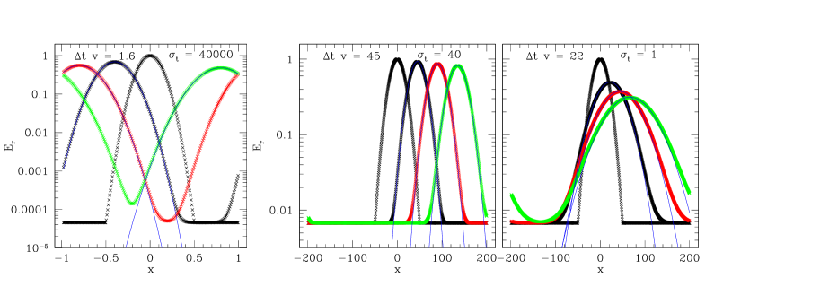
Figure 8.— Dynamic diffusion test for the radiation subsystem with our improved algorithm. From left to right, the parameters for equation A9 are: $\sigma_{t}=40000,\nu^{2}=40$; $\sigma_{t}=40,\nu^{2}=0.002$; $\sigma_{t}=1,\nu^{2}=0.002$. The initial gaussian profiles are all centered at $x=0$. The black dots not centered at $x=0$, the red dots and the green dots are solutions from earlier time to later times with time intervals shown in each panel. The blue lines are analytical solutions (equation A9) at corresponding times, which agree with the analytical solution very well for the regions not close to the boundaries.

In the optically thick regime, the radiation subsystem can be approximated by diffusion equations. In 1D with a constant opacity $\sigma_{t}$ and the Eddington approximation, the diffusion equations and the analytic solution with initial Gaussian pulse for a static medium are given by equations (101) of Sekora & Stone (2010), except that $\sigma_{t}$ only contains scattering opacity here. For the dynamic diffusion test, we let the background fluid move with a constant velocity $v$. In the co-moving frame, the diffusion solution is the same as in the static diffusion case. In the Eulerian frame, the solution is

$$E_{r}(x,t)=\frac{1}{\left(4Dt\nu^{2}+1\right)^{1/2}}\exp\left(\frac{-\left(\nu(x-vt)\right)^{2}}{4Dt\nu^{2}+1}\right),$$ (A9)

with the initial condition

$$E_{r}(x,0)=\exp\left(-\nu^{2}x^{2}\right),\quad\quad F_{r}(x,0)=\frac{2\nu^{2}x}{3\sigma_{t}}E_{r}(x,0)+\frac{4v}{3{\mathbb{C}}}E_{r}(x,0).$$ (A10)

Here $D\equiv{\mathbb{C}}/(3\sigma_{t})$ is the diffusion coefficient and $\nu$ is a free parameter to control the shape of initial Gaussian pulse. We can initialize the Gaussian pulse in the code and compare the analytical and numerical solutions at time $t$. We use periodic boundary conditions so that we do not need very large simulation box when the pulse is advected. The following parameters are chosen for all the tests: ${\mathbb{C}}=514.4$, $v=1$. We test the new algorithm in three cases with different opacities $\sigma_{t}=40000,40,1$. For the first case, the pulse is located within $|x|<0.5$ initially while for the other two cases, the pulse is located within $|x|<50$ initially. Results are shown in Figure 8, which confirms that the improved algorithm can reproduce the diffusion behavior accurately. We have also tried that if we do not use those improvements, the diffusion time is too short compared with what it should be for the pure scattering case.

References

- Agol & Krolik (1998) Agol, E., & Krolik, J. 1998, ApJ, 507, 304
- Audit et al. (2002) Audit, E., Charrier, P., Chièze, J. ., & Dubroca, B. 2002, arXiv:astro-ph/0206281
- Balbus & Hawley (1991) Balbus, S. A., & Hawley, J. F. 1991, ApJ, 376, 214
- Balbus & Hawley (1998) —. 1998, Reviews of Modern Physics, 70, 1
- Balbus & Henri (2008) Balbus, S. A., & Henri, P. 2008, ApJ, 674, 408
- Blackman et al. (2008) Blackman, E. G., Penna, R. F., & Varnière, P. 2008, New Astronomy, 13, 244
- Blaes et al. (2011) Blaes, O., Krolik, J. H., Hirose, S., & Shabaltas, N. 2011, ApJ, 733, 110
- Blaes & Socrates (2001) Blaes, O., & Socrates, A. 2001, ApJ, 553, 987
- Bodo et al. (2008) Bodo, G., Mignone, A., Cattaneo, F., Rossi, P., & Ferrari, A. 2008, A&A, 487, 1
- Castor (2004) Castor, J. I. 2004, Radiation Hydrodynamics, ed. Castor, J. I.
- Davis et al. (2012) Davis, S. W., Stone, J. M., & Jiang, Y.-F. 2012, ApJS, 199, 9
- Davis et al. (2010) Davis, S. W., Stone, J. M., & Pessah, M. E. 2010, ApJ, 713, 52
- Fromang & Papaloizou (2007) Fromang, S., & Papaloizou, J. 2007, A&A, 476, 1113
- Fromang et al. (2007) Fromang, S., Papaloizou, J., Lesur, G., & Heinemann, T. 2007, A&A, 476, 1123
- Gardiner & Stone (2005) Gardiner, T. A., & Stone, J. M. 2005, in American Institute of Physics Conference Series, Vol. 784, Magnetic Fields in the Universe: From Laboratory and Stars to Primordial Structures., ed. E. M. de Gouveia dal Pino, G. Lugones, & A. Lazarian, 475–488
- Goodman & Xu (1994) Goodman, J., & Xu, G. 1994, ApJ, 432, 213
- Guan et al. (2009) Guan, X., Gammie, C. F., Simon, J. B., & Johnson, B. M. 2009, ApJ, 694, 1010
- Hawley et al. (1995) Hawley, J. F., Gammie, C. F., & Balbus, S. A. 1995, ApJ, 440, 742
- Hawley et al. (2011) Hawley, J. F., Guan, X., & Krolik, J. H. 2011, ApJ, 738, 84
- Hirose et al. (2009) Hirose, S., Krolik, J. H., & Blaes, O. 2009, ApJ, 691, 16
- Jiang et al. (2012) Jiang, Y.-F., Stone, J. M., & Davis, S. W. 2012, ApJS, 199, 14
- Latter et al. (2009) Latter, H. N., Lesaffre, P., & Balbus, S. A. 2009, MNRAS, 394, 715
- Lesur & Longaretti (2007) Lesur, G., & Longaretti, P.-Y. 2007, MNRAS, 378, 1471
- Loeb & Laor (1992) Loeb, A., & Laor, A. 1992, ApJ, 384, 115
- Mihalas & Mihalas (1984) Mihalas, D., & Mihalas, B. W. 1984, Foundations of radiation hydrodynamics, ed. Mihalas, D. & Mihalas, B. W.
- Miller & Stone (2000) Miller, K. A., & Stone, J. M. 2000, ApJ, 534, 398
- Pessah & Goodman (2009) Pessah, M. E., & Goodman, J. 2009, ApJ, 698, L72
- Pringle (1981) Pringle, J. E. 1981, ARA&A, 19, 137
- Sano et al. (2004) Sano, T., Inutsuka, S.-i., Turner, N. J., & Stone, J. M. 2004, ApJ, 605, 321
- Sekora & Stone (2010) Sekora, M. D., & Stone, J. M. 2010, Journal of Computational Physics, 229, 6819
- Shakura & Sunyaev (1973) Shakura, N. I., & Sunyaev, R. A. 1973, A&A, 24, 337
- Simon & Hawley (2009) Simon, J. B., & Hawley, J. F. 2009, ApJ, 707, 833
- Simon et al. (2009) Simon, J. B., Hawley, J. F., & Beckwith, K. 2009, ApJ, 690, 974
- Sorathia et al. (2012) Sorathia, K. A., Reynolds, C. S., Stone, J. M., & Beckwith, K. 2012, ApJ, 749, 189
- Stone & Gardiner (2010) Stone, J. M., & Gardiner, T. A. 2010, ApJS, 189, 142
- Stone et al. (2008) Stone, J. M., Gardiner, T. A., Teuben, P., Hawley, J. F., & Simon, J. B. 2008, ApJS, 178, 137
- Stone et al. (1996) Stone, J. M., Hawley, J. F., Gammie, C. F., & Balbus, S. A. 1996, ApJ, 463, 656
- Stone & Norman (1992) Stone, J. M., & Norman, M. L. 1992, ApJS, 80, 753
- Turner (2004) Turner, N. J. 2004, ApJ, 605, L45
- Turner & Stone (2001) Turner, N. J., & Stone, J. M. 2001, ApJS, 135, 95
- Turner et al. (2003) Turner, N. J., Stone, J. M., Krolik, J. H., & Sano, T. 2003, ApJ, 593, 992