Integral and Series Representations
of the Dirac Delta Function

Abstract.

Mathematical justifications are given for several integral and series representations of the Dirac delta function which appear in the physics literature. These include integrals of products of Airy functions, and of Coulomb wave functions; they also include series of products of Laguerre polynomials and of spherical harmonics. The methods used are essentially based on the asymptotic behavior of these special functions.

Y. T. Li

Department of Mathematics, City University of Hong Kong,

Tat Chee Avenue, Kowloon, Hong Kong.

R. Wong

Liu Bie Ju Centre for Mathematical Sciences, City University of Hong Kong,

Tat Chee Avenue, Kowloon, Hong Kong.

1. Introduction

The Dirac delta function $\delta(x)$ has been used in physics well before the theory of distributions (generalized functions) was introduced by mathematicians. The manner in which physicists used this function was to define it by the equations

(1.1) $$\delta(x-a)=0,\qquad\qquad x\neq a,$$

and

(1.2) $$\int^{\infty}_{-\infty}\phi(x)\delta(x-a)dx=\phi(a),\qquad\qquad a\in\mathbb{R},$$

for any continuous function $\phi(x)$ on $\mathbb{R}$. However, mathematically, these two equations are inconsistent in the classical sense of a function and an integral, since the value of the integral of a function which is zero everywhere except for a finite number of points should be zero. There are now two mathematically meaningful approaches to help us interpret the delta function given in $(1.1)-(1.2)$. One approach is to consider $\delta_{a}:=\delta(x-a)$ as a continuous linear functional acting on a space of smooth functions with rapid decay at $\pm\infty$, and the action of $\delta_{a}$ on a particular function $\phi(x)$ is given the value $\phi(a)$; see [14, p.141] and [15, p.77]. The other approach is to find a sequence of functions $\delta_{n}(x-a)$ such that

(1.3) $$\lim_{n\to\infty}\int^{\infty}_{-\infty}\delta_{n}(x-a)\phi(x)dx=\phi(a),\qquad\qquad a\in\mathbb{R};$$

see [7, p.55] and [10, p.17]. Such a sequence is called a delta sequence and we write, symbolically,

(1.4) $$\lim_{n\to\infty}\delta_{n}(x-a)=\delta(x-a),\qquad\qquad x\in\mathbb{R}.$$

It seems that the second approach is more acceptable to physicists and applied mathematicians.

Recently, in the process of preparing some material for the major project “NIST Handbook of Mathematical Functions [13]”, we encountered some very interesting integral and series representations of the delta function which need mathematical justification. For instance, in [3, p.696] the formula

(1.5) $$\int^{\infty}_{0}xtJ_{\nu}(xt)J_{\nu}(at)dt=\delta(x-a),\qquad\qquad\textup{Re}\;\nu>-1,\;\;x>0,\;\;a>0,$$

appears, where $J_{\nu}(x)$ is the Bessel function of the first kind, and in [16, Eq.(122)] one finds the integral representation

(1.6) $$\int^{\infty}_{0}s(x,l;t)s(a,l;t)dt=\delta(x-a),\qquad\qquad a>0,\;\;x>0,$$

where $s(x,l;t)$ is the Coulomb wave function. A recent reference [17, p.57] on the Airy function $\textup{Ai}(x)$ also gives the formula

(1.7) $$\int^{\infty}_{-\infty}\textup{Ai}(t-x)\textup{Ai}(t-a)dt=\delta(x-a).$$

While physicists may find these representations convenient to use in applications, mathematicians would, in general, feel uneasy or even disturbed to see these formulas being used since the integrals in $(1.5)-(1.7)$ are all divergent. Thus, it would seem meaningful and necessary to give a mathematical justification for these representations, and this is exactly the purpose of the present paper.

There are also some series representations for the delta function. These include the following:

(1.8) $$\sum^{\infty}_{k=0}\biggl{(}k+\frac{1}{2}\biggr{)}P_{k}(x)P_{k}(a)=\delta(x-a),$$

(1.9) $$\frac{e^{-(x^{2}+a^{2})/2}}{\sqrt{\pi}}\sum^{\infty}_{k=0}\frac{1}{2^{k}k!}H_{k}(x)H_{k}(a)=\delta(x-a),$$

and

(1.10) $$e^{-(x+a)/2}\sum^{\infty}_{k=0}L_{k}(x)L_{k}(a)=\delta(x-a),$$

where $P_{k}(x)$, $H_{k}(x)$ and $L_{k}(x)$ are, respectively, the Legendre, Hermite and Laguerre polynomials. Equations $(1.8)-(1.10)$ are special cases of an equation in Morse and Feshbach [11, p.729]. Another series representation is given in [3, p.792]; that is,

(1.11) $$\begin{split}\sum^{\infty}_{k=0}\sum^{k}_{l=-k}Y_{kl}(\theta_{1},\phi_{1})Y^{*}_{kl}(\theta_{2},\phi_{2})&=\frac{1}{\sin\theta_{1}}\delta(\theta_{1}-\theta_{2})\delta(\phi_{1}-\phi_{2})\\ &=\delta(\cos\theta_{1}-\cos\theta_{2})\delta(\phi_{1}-\phi_{2}),\end{split}$$

where the functions $Y_{kl}(\theta,\phi)$ are the spherical harmonics (see [3, p.788]) and the asterisk “$\ast$” denotes complex conjugate.

The orthogonal polynomials in $(1.8)-(1.10)$ and the orthogonal function in (1.11) are the eigenfunctions corresponding to the eigenvalues (discrete spectrum) of some differential operators. Likewise, the special functions in $(1.5)-(1.7)$ can be regarded as the eigenfunctions associated with the continuous spectrum of corresponding differential operators. The proofs of the representations in $(1.8)-(1.11)$ turn out to be much simpler than the proofs of those in $(1.5)-(1.7)$. Indeed, we shall show that the results in $(1.8)-(1.11)$ all follow from expansion theorems in orthogonal polynomials, whereas for the representations in $(1.5)-(1.7)$ we need to provide some new arguments.

2. A generalized Riemann-Lebesgue Lemma

There are already several delta sequences in the literature. For instance, we have

(2.1) $$\delta_{n}(x-a)=\sqrt{\dfrac{n}{\pi}}e^{-n(x-a)^{2}},$$

(2.2) $$\delta_{n}(x-a)=\dfrac{n}{\pi}\dfrac{1}{1+n^{2}(x-a)^{2}},$$

and

(2.3) $$\delta_{n}(x-a)=\frac{1}{\pi}\frac{\sin n(x-a)}{x-a};$$

see [5, pp. 35-38] and [8, pp. 5-13]. To verify whether a given sequence of functions is a delta sequence, one can apply the criteria given in [5, p.34]. If the function $\phi(x)$ in (1.3) is only piecewise continuous in $\mathbb{R}$, then this equation becomes

(2.4) $$\lim_{n\to\infty}\int^{\infty}_{-\infty}\delta_{n}(x-a)\phi(x)dx=\frac{1}{2}[\phi(a^{+})+\phi(a^{-})],\qquad\qquad a\in\mathbb{R};$$

see [8, p.16].

For convenience in our later argument, we also state and prove the following result.

Lemma.

(A generalized Riemann-Lebesgue lemma). Let $g(x,R)$ be a continuous function of $x\in(A,B)$ and uniformly bounded for $R>0$. If

(2.5) $$\lim_{R\to\infty}\int^{B^{\prime}}_{A^{\prime}}g(x,R)dx=0$$

for any $A^{\prime}$ and $B^{\prime}$ with $A<A^{\prime}<B^{\prime}<B$, then

(2.6) $$\lim_{R\to\infty}\int^{B}_{A}\psi(x)g(x,R)dx=0$$

for any integrable function $\psi(x)$ on the finite interval $(A,B)$. If $A=0$ and $B=+\infty$, or if $A=-\infty$ and $B=+\infty$, then (2.6) holds for any absolutely integrable function $\psi(x)$ on the infinite interval $(A,B)$.

Proof.

First, from (2.5) it is easy to see that (2.6) holds for step functions. Now, let $\psi(x)$ be an integrable function on $(A,B)$. For any $\varepsilon>0$, we can always find a step function $s(x)$ such that

(2.7) $$\int^{B}_{A}|\psi(x)-s(x)|\,dx<\frac{\varepsilon}{2K},$$

where $K=\max\{|g(x,R)|:x\in\mathbb{R}\;\textup{and}\;R>0\}$. Choose $R_{0}>0$ so that

(2.8) $$\biggl{|}\int^{B}_{A}s(x)g(x,R)dx\biggr{|}<\frac{\varepsilon}{2}\qquad\qquad\textup{for all}\;R\geq R_{0}.$$

Write

$$\int^{B}_{A}\psi(x)g(x,R)dx=\int^{B}_{A}[\psi(x)-s(x)]g(x,R)dx+\int^{B}_{A}s(x)g(x,R)dx.$$

On account of (2.7) and (2.8), we have

$$\biggl{|}\int^{B}_{A}\phi(x)g(x,R)dx\biggr{|}<\varepsilon$$

for all $R\geq R_{0}$. Since $\varepsilon$ is arbitrary, this proves (2.6) when $A$ and $B$ are finite.

If the interval of integration is infinite, and if $\psi(x)$ is absolutely integrable there, then we can choose finite numbers $A$ and $B$ such that the integral $\int\psi(x)g(x,R)dx$ outside the interval $(A,B)$ is small since $g(x,R)$ is uniformly bounded. On the finite interval $(A,B)$, we can apply the result just established. ∎

3. Bessel function

The Bessel function $J_{\nu}(xt)$ is a solution of the differential equation

(3.1) $$\frac{d}{dt}\biggl{(}t\frac{dy}{dt}\biggr{)}+\biggl{(}x^{2}t-\frac{\nu^{2}}{t}\biggr{)}y=0.$$

With $x$ replaced by $a$, one obtains a corresponding equation for $J_{\nu}(at)$. Multiplying equation (3.1) by $J_{\nu}(at)$ and the corresponding equation for $J_{\nu}(at)$ by $J_{\nu}(xt)$, and subtracting the two resulting equations, leads to

(3.2) $$\begin{split}(x^{2}-a^{2})tJ_{\nu}(at)J_{\nu}(xt)=\frac{d}{dt}\{&atJ_{\nu}(xt)J^{\prime}_{\nu}(at)\\ &-xtJ_{\nu}(at)J^{\prime}_{\nu}(xt)\}.\end{split}$$

Put

(3.3) $$\delta_{R}(x,a)=x\int^{R}_{0}J_{\nu}(xt)J_{\nu}(at)t\,dt.$$

An integration of (3.2) gives

(3.4) $$\delta_{R}(x,a)=\frac{x}{x^{2}-a^{2}}\biggl{[}at\,J_{\nu}(xt)J^{\prime}_{\nu}(at)-xt\,J_{\nu}(at)J^{\prime}_{\nu}(xt)\biggr{]}^{R}_{0}.$$

From the ascending power series representation

(3.5) $$J_{\nu}(t)=\biggl{(}\frac{t}{2}\biggr{)}^{\nu}\sum^{\infty}_{n=0}\frac{(-1)^{n}}{\Gamma(n+\nu+1)n!}\biggl{(}\frac{t}{2}\biggr{)}^{{2n}},$$

it can be shown that the leading terms in the series expansions of $at\,J_{\nu}(xt)J^{\prime}_{\nu}(at)$ and $xt\,J_{\nu}(at)J^{\prime}_{\nu}(xt)$ cancel out. Thus, the right-hand side of (3.4) vanishes at the lower limit when $\nu>-1$, and we obtain

(3.6) $$\delta_{R}(x,a)=\frac{x}{x^{2}-a^{2}}[aRJ_{\nu}(xR)J^{\prime}_{\nu}(aR)-xRJ_{\nu}(aR)J^{\prime}_{\nu}(xR)].$$

Theorem 1.

For $a>0$, $\nu>-1$ and any piecewise continuously differentiable function $\phi(x)$ on $(0,\infty)$, we have

(3.7) $$\lim_{R\to\infty}\int^{\infty}_{0}\phi(x)x\biggl{(}\int^{R}_{0}J_{\nu}(xt)J_{\nu}(at)t\;dt\biggr{)}dx=\frac{1}{2}[\phi(a^{+})+\phi(a^{-})],$$

provided that

(i) $\int^{\infty}_{1}x^{-\frac{1}{2}}|\phi(x)|dx$ converges;
(ii) $\int^{1}_{0}x^{\frac{1}{2}}|\phi(x)|dx$ converges when $\nu\geq-\frac{1}{2}$, or
(ii^′) $\int^{1}_{0}x^{\nu+1}|\phi(x)|dx$ converges when $-1<\nu<-\frac{1}{2}$.

Proof.

In view of the asymptotic formulas

(3.8) $$J_{\nu}(xt)=\sqrt{\frac{2}{\pi xt}}\biggl{[}\cos\biggl{(}xt-\frac{\nu\pi}{2}-\frac{\pi}{4}\biggr{)}+\varepsilon_{1}(x,t)\biggr{]}$$

and

(3.9) $$J^{\prime}_{\nu}(xt)=-\sqrt{\frac{2}{\pi xt}}\biggl{[}\sin\biggl{(}xt-\frac{\nu\pi}{2}-\frac{\pi}{4}\biggr{)}+\varepsilon_{2}(x,t)\biggr{]}$$

where $\varepsilon_{j}(x,t)=O(1/t)$ as $t\to\infty$ uniformly for $x\geq\delta>0$ and $j=1,2$, there are constants $M_{1}>0$ and $M_{2}>0$ such that

(3.10) $$|J_{\nu}(aR)|\leq M_{1}R^{-\frac{1}{2}},\qquad\qquad|J^{\prime}_{\nu}(aR)|\leq M_{1}R^{-\frac{1}{2}}$$

and

(3.11) $$|J_{\nu}(xR)|\leq M_{2}x^{-\frac{1}{2}}R^{-\frac{1}{2}},\qquad\qquad|J^{\prime}_{\nu}(xR)|\leq M_{2}x^{-\frac{1}{2}}R^{-\frac{1}{2}}$$

for $x\geq 1$ and $R\geq 1$. From (3.6), it follows that

$$|\delta_{R}(x,a)|\leq M_{1}M_{2}\frac{x^{2}}{|x^{2}-a^{2}|}\biggl{(}\frac{a}{x^{3/2}}+\frac{1}{x^{1/2}}\biggr{)}.$$

Hence, for $b>\max\{a,1\}$, we have

$$\int^{\infty}_{b}|\delta_{R}(x,a)\phi(x)|dx\leq M_{3}\int^{\infty}_{b}x^{-\frac{1}{2}}|\phi(x)|dx,$$

where $M_{3}=M_{1}M_{2}(a+1)b^{2}/(b^{2}-a^{2})$. Since the last integral is convergent by condition (i), for any $\varepsilon>0$ there exists a number $c>b$ such that

(3.12) $$\int^{\infty}_{c}|\delta_{R}(x,a)\phi(x)|dx<\frac{\varepsilon}{2}.$$

Let $0<\rho<\min\{a,1\}$. To estimate the integral of $\delta_{R}(x,a)\phi(x)$ on the interval $(0,\rho)$, we divide our discussion into two cases: (i) $\nu\geq-\frac{1}{2}$, and (ii) $-1<\nu<-\frac{1}{2}$. In the first case, we have from (3.5) a positive constant $M^{\prime}_{4}$ such that

(3.13a) $$|J_{\nu}(xR)|\leq M^{\prime}_{4}(xR)^{\nu}\leq M^{\prime}_{4}(xR)^{-\frac{1}{2}}$$

and

(3.13b) $$|J^{\prime}_{\nu}(xR)|\leq M^{\prime}_{4}(xR)^{\nu-1}\leq M^{\prime}_{4}x^{-\frac{3}{2}}R^{-\frac{3}{2}}\leq M^{\prime}_{4}x^{-\frac{3}{2}}R^{-\frac{1}{2}}$$

for $0<xR\leq 1$ and $R\geq 1$. From (3.8) and (3.9), we also have

(3.14) $$|J_{\nu}(xR)|\leq M^{\prime\prime}_{4}x^{-\frac{1}{2}}R^{-\frac{1}{2}},\qquad\qquad|J^{\prime}_{\nu}(xR)|\leq M^{\prime\prime}_{4}x^{-\frac{1}{2}}R^{-\frac{1}{2}}$$

for $xR\geq 1$. Coupling (3.13) and (3.14), we obtain

$$|J_{\nu}(xR)|\leq M_{4}x^{-\frac{1}{2}}R^{-\frac{1}{2}},\qquad\qquad|J^{\prime}_{\nu}(xR)|\leq M_{4}x^{-\frac{3}{2}}R^{-\frac{1}{2}}$$

for $0<x\leq 1$ and $R\geq 1$, with $M_{4}=\max\{M^{\prime}_{4},M^{\prime\prime}_{4}\}$. Thus,

$$|\delta_{R}(x,a)|\leq M_{1}M_{4}(a+1)\frac{x^{\frac{1}{2}}}{a^{2}-\rho^{2}},\qquad\qquad 0<x\leq 1,$$

and

(3.15) $$\int^{\rho}_{0}|\delta_{R}(x,a)\phi(x)|dx\leq M_{5}\int^{\rho}_{0}x^{\frac{1}{2}}|\phi(x)|dx,$$

where $M_{5}=M_{1}M_{4}(a+1)/(a^{2}-\rho^{2})$.

In the second case, there are constants $M^{\prime}_{6}>0$ and $M^{\prime\prime}_{6}>0$ such that

$$\begin{split}&\hskip 17.07164pt|J_{\nu}(xR)|\leq M^{\prime}_{6}(xR)^{\nu}\leq M^{\prime}_{6}x^{\nu}R^{-\frac{1}{2}},\\ &|J^{\prime}_{\nu}(xR)|\leq M^{\prime}_{6}(xR)^{\nu-1}\leq M^{\prime}_{6}x^{\nu-1}R^{-\frac{1}{2}}\end{split}$$

for $0<xR\leq 1$ and $R\geq 1$, and

$$\begin{split}&|J_{\nu}(xR)|\leq M^{\prime\prime}_{6}x^{-\frac{1}{2}}R^{-\frac{1}{2}}\leq M^{\prime\prime}_{6}x^{\nu}R^{-\frac{1}{2}},\\ &|J^{\prime}_{\nu}(xR)|\leq M^{\prime\prime}_{6}x^{-\frac{1}{2}}R^{-\frac{1}{2}}\leq M^{\prime\prime}_{6}x^{\nu-1}R^{-\frac{1}{2}}\end{split}$$

for $xR\geq 1$ and $R\geq 1$. With $M_{6}=\max\{M^{\prime}_{6},M^{\prime\prime}_{6}\}$, it follows that

$$|J_{\nu}(xR)|\leq M_{6}x^{\nu}R^{-\frac{1}{2}}\qquad\textup{and}\qquad|J^{\prime}_{\nu}(xR)|\leq M_{6}x^{\nu-1}R^{-\frac{1}{2}}.$$

Therefore,

$$|\delta_{R}(x,a)|\leq M_{1}M_{6}\frac{1}{a^{2}-\rho^{2}}(a+1)x^{\nu+1}$$

and

(3.16) $$\int^{\rho}_{0}|\delta_{R}(x,a)\phi(x)|dx\leq M_{7}\int^{\rho}_{0}x^{\nu+1}|\phi(x)|dx,$$

where $M_{7}=M_{1}M_{6}(a+1)/(a^{2}-\rho^{2})$. On account of conditions (ii) and (ii^′), for any $\varepsilon>0$ there is a constant $0<d<\rho$ such that

(3.17) $$\int^{d}_{0}|\delta_{R}(x,a)\phi(x)|dx<\frac{\varepsilon}{2}.$$

For $d<x<c$, a combination of (3.6), (3.8) and (3.9) gives

(3.18) $$\begin{split}\delta_{R}(x,a)=\frac{2}{\pi}\frac{x}{x^{2}-a^{2}}\biggl{\{}&\sqrt{\frac{x}{a}}\sin\zeta(x,R)\cos\zeta(a,R)\\ &-\sqrt{\frac{a}{x}}\cos\zeta(x,R)\sin\zeta(a,R)+\varepsilon(x,a;R)\biggr{\}},\end{split}$$

where $c$ and $d$ are given in (3.12) and (3.17), respectively, $\zeta(x,R)=xR-\frac{\nu\pi}{2}-\frac{\pi}{4}$ and $\varepsilon(x,a;R)=O(1/R)$ as $R\to\infty$ uniformly for $x\in(d,c)$. Note that $\varepsilon(x,a;R)$ is continuously differentiable, $\varepsilon(x,a;R)/(x-a)$ is continuous in $x$ and uniformly bounded in $x$ and $R$, and $\phi(x)$ is piecewise continuous in $(d,c)$. Hence,

(3.19) $$\lim_{R\to\infty}\int^{c}_{d}\frac{\varepsilon(x,a;R)}{x^{2}-a^{2}}x\phi(x)dx=0.$$

By the Riemann-Lebesgue lemma, we also have

(3.20) $$\lim_{R\to\infty}\int^{c}_{d}\biggl{(}\sqrt{\frac{x}{a}}-1\biggr{)}\frac{\sin\zeta(x,R)}{x^{2}-a^{2}}x\phi(x)dx=0$$

and

(3.21) $$\lim_{R\to\infty}\int^{c}_{d}\biggl{(}\sqrt{\frac{a}{x}}-1\biggr{)}\frac{\cos\zeta(x,R)}{x^{2}-a^{2}}x\phi(x)dx=0.$$

A combination of the results in $(3.18)-(3.21)$ yields

$$\begin{split}\lim_{R\to\infty}\int^{c}_{d}\delta_{R}(x,a)\phi(x)dx&=\lim_{R\to\infty}\frac{2}{\pi}\int^{c}_{d}\frac{\sin\{\zeta(x,R)-\zeta(a,R)\}}{x^{2}-a^{2}}x\phi(x)dx\\ &=\lim_{R\to\infty}\int^{c}_{d}\frac{\sin R(x-a)}{\pi(x-a)}\cdot\frac{2x}{x+a}\phi(x)dx\end{split}$$

On account of Jordan’s theorem on the Dirichlet kernel [2, p.473], we conclude

(3.22) $$\lim_{R\to\infty}\int^{c}_{d}\delta_{R}(x,a)\phi(x)dx=\frac{1}{2}[\phi(a^{-})+\phi(a^{+})].$$

Since the number $\varepsilon$ in (3.12) and (3.17) is arbitrary, it follows from (3.22) that

$$\lim_{R\to\infty}\int^{\infty}_{0}\delta_{R}(x,a)\phi(x)dx=\frac{1}{2}[\phi(a^{-})+\phi(a^{+})],$$

which is equivalent to (3.7). ∎

4. Coulomb wave function

The Coulomb wave function $s(x,l;r)$ is a solution of the Coulomb wave equation

(4.1) $$\frac{d^{2}y}{dr^{2}}+\biggl{\{}x+\biggl{(}\frac{2}{r}-\frac{l(l+1)}{r^{2}}\biggr{)}\biggr{\}}y=0,$$

that satisfies the initial conditions

(4.2) $$s(x,l;0)=s^{\prime}(x,l;0)=0$$

and has the asymptotic behavior

(4.3) $$s(x,l;r)=\dfrac{1}{\sqrt{\pi}}x^{-\frac{1}{4}}[\sin\zeta(x,l;r)+\varepsilon_{1}(x,l;r)],$$

(4.4) $$s^{\prime}(x,l;r)=\dfrac{1}{\sqrt{\pi}}x^{\frac{1}{4}}[\cos\zeta(x,l;r)+\varepsilon_{2}(x,l;r)],$$

where $\varepsilon_{j}(x,l;r)=O(1/r)$ as $r\to\infty$ uniformly for $x\geq\delta>0,j=1,2$, and

(4.5) $$\zeta(x,l;r)=kr+\frac{1}{k}\textup{ln}\;(2kr)-\frac{l\pi}{2}+\arg\Gamma\biggl{(}l+1-\frac{i}{k}\biggr{)}$$

with $k=\sqrt{x}$; see [16, p.236]. For $a>0$ and $x>0$, we define

(4.6) $$\delta_{R}(x,a)=\int^{R}_{0}s(x,l;r)s(a,l;r)dr.$$

From (4.1) and (4.2), one can show as in Sec. 3 that

(4.7) $$\delta_{R}(x,a)=\frac{s(x,l;R)s^{\prime}(a,l;R)-s^{\prime}(x,l;R)s(a,l;R)}{x-a}.$$

Theorem 2.

For any $a>0$ and any piecewise continuously differentiable function $\phi(x)$ on $(0,\infty)$, we have

(4.8) $$\lim_{R\to\infty}\int^{\infty}_{0}\phi(x)\int^{R}_{0}s(x,l;r)s(a,l;r)dr\,dx=\frac{1}{2}[\phi(a^{+})+\phi(a^{-})],$$

provided that the integrals

(4.9) $$\int^{1}_{0}x^{-\frac{1}{4}}|\phi(x)|dx\qquad and\qquad\int^{\infty}_{1}x^{-\frac{3}{4}}|\phi(x)|dx$$

are convergent.

Proof.

From formulas (4.3) and (4.4), for any $b>\max\{a,1\}$ there exists a number $M_{1}>0$ such that

$$\begin{split}&|s(x,l;R)s^{\prime}(a,l;R)|\leq M_{1}x^{-\frac{1}{4}},\\ &|s^{\prime}(x,l;R)s(a,l;R)|\leq M_{1}x^{\frac{1}{4}}\end{split}$$

for $R\geq 1$ and $x\geq b$. Hence, it follows from (4.7) that

$$\int^{\infty}_{b}|\delta_{R}(x,a)\phi(x)|dx\leq 2M_{1}\int^{\infty}_{b}\frac{x^{\frac{1}{4}}|\phi(x)|}{x-a}dx\leq M_{2}\int^{\infty}_{b}x^{-\frac{3}{4}}|\phi(x)|dx,$$

where $M_{2}=2bM_{1}/(b-a)$. By hypothesis, the last integral is convergent; so for any $\varepsilon>0$ there is a number $c>b$ such that

(4.10) $$\int^{\infty}_{c}|\delta_{R}(x,a)\phi(x)|dx<\frac{\varepsilon}{2}\qquad\qquad\textup{for all}\;R\geq 1.$$

To prove that there exists a number $d>0$ such that

(4.11) $$\int^{d}_{0}|\delta_{R}(x,a)\phi(x)|dx<\frac{\varepsilon}{2}\qquad\qquad\textup{for all}\;R\geq 1,$$

we first need to demonstrate that

(4.12) $$k^{\frac{1}{2}}s(k^{2},l;r)=O(1)\qquad\qquad\textup{as}\;r\to\infty,$$

(4.13) $$s^{\prime}(k^{2},l;r)=O(1)\qquad\qquad\textup{as}\;r\to\infty,$$

uniformly for all sufficiently small $k\geq 0$. (Recall: $k=\sqrt{x}$.) This can be done by considering two separate cases: (i) $kr\to\infty$, and (ii) $kr$ bounded. In case (i), we first make the change of variable $\rho=kr$ and set $\omega(\rho)=y(\rho/k)=y(r)$ so that equation (4.1) becomes

(4.14) $$\frac{d^{2}\omega}{d\rho^{2}}+\biggl{(}1+\frac{2}{k\rho}-\frac{l(l+1)}{\rho^{2}}\biggr{)}\omega=0,$$

and then apply the Liouville-Green transformation given in [12, p.196] with $f(\rho)=1+(2/k\rho)$ and $g(\rho)=l(l+1)/\rho^{2}$. The result is that equation (4.14) has a solution $\omega_{1}(k;\rho)$ such that

(4.15) $$\omega_{1}(k;\rho)\sim\biggl{(}1+\frac{2}{k\rho}\biggr{)}^{-\frac{1}{4}}\sin\biggl{\{}\int\biggl{(}1+\frac{2}{k\rho}\biggr{)}^{\frac{1}{2}}d\rho\biggr{\}}\qquad\qquad\textup{as}\;\rho\to\infty$$

and

(4.16) $$\frac{d}{d\rho}\omega_{1}(k;\rho)\sim\biggl{(}1+\frac{2}{k\rho}\biggr{)}^{\frac{1}{4}}\cos\biggl{\{}\int\biggl{(}1+\frac{2}{k\rho}\biggr{)}^{\frac{1}{2}}d\rho\biggr{\}}\qquad\qquad\textup{as}\;\rho\to\infty.$$

With a suitable choice of the integration constant and for fixed $k>0$, we have

$$\int\biggl{(}1+\frac{2}{k\rho}\biggr{)}^{\frac{1}{2}}d\rho=\zeta^{*}(k,l;\rho)+O\biggl{(}\frac{1}{\rho}\biggr{)}\qquad\qquad\textup{as}\;\rho\to\infty,$$

where

$$\zeta^{*}(k,l;\rho)=\rho+\frac{1}{k}\ln 2\rho-\frac{l\pi}{2}+\arg\Gamma\biggl{(}l+1-\frac{i}{k}\biggr{)}$$

which is exactly equal to the function $\zeta(k^{2},l;r)$ given in (4.5). For fixed $k>0$, we can compare the behavior of $s(k^{2},l;r)$ given in (4.3) and that given in (4.15). The conclusion is

(4.17) $$s(k^{2},l;r)=\frac{1}{\sqrt{\pi k}}\omega_{1}(k;\rho),$$

from which we also obtain

(4.18) $$s^{\prime}(k^{2},l;r)=\sqrt{\frac{k}{\pi}}\frac{d\omega_{1}}{d\rho}.$$

Since $\omega_{1}(k;\rho)=O(1)$ and $\omega^{\prime}_{1}(k;\rho)=O(k^{-\frac{1}{4}})$ for all small $k$ and large $\rho$ on account of (4.15) and (4.16), the order estimates in (4.12) and (4.13) are established.

In case (ii), we first recall the function

$$f(k^{2},l;r)=\frac{(i/k)^{l+1}}{\Gamma(2l+2)}M_{i/k,l+\frac{1}{2}}(-2ikr),$$

where $M_{\kappa,\lambda}(z)$ is a Whittaker function; see Seaton [16, eqs. (14) & (22)]. This function is related to the Coulomb wave function $s(k^{2},l;r)$ via

$$s(k^{2},l;r)=\biggl{[}\frac{A(k^{2},l)}{2(1-e^{-2\pi/k})}\biggr{]}^{\frac{1}{2}}f(k^{2},l;r),$$

where $A(k^{2},l)$ is a polynomial of degree $l$ in $k^{2}$; see [16, eq.(114)]. In view of the convergent expansion [4, $\S$ 7, eq.(16)]

$$M_{\kappa,\lambda}(z)=\Gamma(2\lambda+1)2^{2\lambda}z^{\lambda+\frac{1}{2}}\sum^{\infty}_{n=0}p^{(2\lambda)}_{n}(z)\frac{J_{2\lambda+n}(2\sqrt{z\kappa})}{(2\sqrt{z\kappa})^{2\lambda+n}},$$

where the $p^{(2\lambda)}_{n}(z)$ are polynomials in $z^{2}$, we have for bounded $kr$

$$f(k^{2},l;r)=C(kr)r^{\frac{1}{4}}\cos\biggl{(}2\sqrt{2r}-\frac{\pi}{2}(2l+1)-\frac{1}{4}\pi\biggr{)}+O\biggl{(}\frac{1}{r^{1/4}}\biggr{)}$$

as $r\to\infty$, where $C(kr)$ is a polynomial of $kr$. Hence,

(4.19) $$\begin{split}s(k^{2},l;r)&=C^{*}(kr)k^{-\frac{1}{4}}\biggl{[}\frac{A(k^{2},l)}{2(1-e^{-2\pi/k})}\biggr{]}^{\frac{1}{2}}\cos\biggl{(}2\sqrt{2r}-\frac{\pi}{2}(2l+1)-\frac{1}{4}\pi\biggr{)}\\ &\hskip 10.81204pt+O\biggl{(}\frac{1}{r^{1/4}}\biggr{)}\end{split}$$

and

(4.20) $$\begin{split}s^{\prime}(k^{2},l;r)&=-C(kr)r^{-\frac{1}{4}}\biggl{[}\frac{A(k^{2},l)}{(1-e^{-2\pi/k})}\biggr{]}^{\frac{1}{2}}\sin\biggl{(}2\sqrt{2r}-\frac{\pi}{2}(2l+1)-\frac{1}{4}\pi\biggr{)}\\ &\hskip 10.81204pt+O\biggl{(}\frac{1}{r^{3/4}}\biggr{)},\end{split}$$

where $C^{*}(kr)=(kr)^{\frac{1}{4}}C(kr)$, again proving (4.12) and (4.13).

From (4.12) and (4.13), it follows that there are constants $0<\rho<\min\{a,1\}$, $R_{0}>0$ and $N_{1}>0$ such that

$$|x^{\frac{1}{4}}s(x,l;r)|\leq N_{1}\qquad\textup{and}\qquad|s^{\prime}(x,l;r)|\leq N_{1}$$

for all $r\geq R_{0}$ and $0\leq x\leq\rho$. Furthermore, by (4.7),

$$|\delta_{R}(x,a)|\leq\frac{N^{2}_{1}}{|x-a|}(x^{-\frac{1}{4}}+a^{-\frac{1}{4}})\leq 2N^{2}_{1}\frac{x^{-\frac{1}{4}}}{|x-a|}$$

for $0<x\leq\rho$ and $R\geq R_{0}$, and

$$\int^{\rho}_{0}|\delta_{R}(x,a)\phi(x)|dx\leq N_{2}\int^{\rho}_{0}x^{-\frac{1}{4}}|\phi(x)|dx,$$

where $N_{2}=2N_{1}^{2}/(a-\rho)$. By hypothesis, the last integral is convergent, thus establishing (4.11).

Let us now consider the case when $x$ lies in the interval $(d,c)$. From (4.3), (4.4) and (4.7), we have

(4.21) $$\begin{split}\pi(x-a)\delta_{R}(x,a)&=\biggl{(}\frac{a}{x}\biggr{)}^{\frac{1}{4}}\sin\zeta(x,l;R)\cos\zeta(a,l;R)\\ &\hskip 14.22636pt-\biggl{(}\frac{x}{a}\biggr{)}^{\frac{1}{4}}\cos\zeta(x,l;R)\sin\zeta(a,l;R)+\varepsilon(x,a;R),\end{split}$$

where $\varepsilon(x,a;R)/(x-a)$ is continuous in $(0,\infty)$ and $\varepsilon(x,a;R)=O(1/R)$ as $R\to\infty$ uniformly for $x\in(d,c)$. As a consequence, we obtain

(4.22) $$\lim_{R\to\infty}\int^{c}_{d}\frac{\varepsilon(x,a;R)}{x-a}\phi(x)dx=0.$$

For any $A$ and $B$ satisfying $d\leq A<B\leq c$, an integration by parts yields

$$\begin{split}\int^{B}_{A}\sin\zeta(k^{2},l;R)dk&=-\frac{\cos\zeta(k^{2},l;R)}{\zeta_{k}(k^{2},l;R)}\biggl{|}^{B}_{A}\\ &\hskip 11.38109pt+\int^{B}_{A}\frac{\partial}{\partial k}\biggl{(}\frac{1}{\zeta_{k}(k^{2},l;R)}\biggr{)}\cos\zeta(k^{2},l;R)dk,\end{split}$$

where $\zeta_{k}(k^{2},l;R)$ denotes the derivative of $\zeta(k^{2},l;R)$ with respect to $k$. From (4.5), it is readily seen that for $d\leq k^{2}\leq c$,

$$\zeta_{k}(k^{2},l;R)\to\infty\qquad\textup{and}\qquad\frac{\partial}{\partial k}\biggl{(}\frac{1}{\zeta_{k}(k^{2},l;R)}\biggr{)}\to 0$$

as $R\to\infty$. Hence,

(4.23) $$\lim_{R\to\infty}\int^{B}_{A}\sin\zeta(k^{2},l;R)dk=0.$$

Similarly, we also have

(4.24) $$\lim_{R\to\infty}\int^{B}_{A}\cos\zeta(k^{2},l;R)dk=0.$$

Let $\eta>0$ be an arbitrary number such that $d<a-\eta<a+\eta<c$. A combination of (4.23), (4.24) and the generalized Riemann-Lebesgue lemma gives

(4.25) $$\lim_{R\to\infty}\biggl{(}\int^{a-\eta}_{d}+\int^{c}_{a+\eta}\biggr{)}\biggl{(}\frac{a}{x}\biggr{)}^{\frac{1}{4}}\frac{\phi(x)}{x-a}\sin\zeta(x,l;R)dx=0$$

and

(4.26) $$\lim_{R\to\infty}\biggl{(}\int^{a-\eta}_{d}+\int^{c}_{a+\eta}\biggr{)}\biggl{(}\frac{x}{a}\biggr{)}^{\frac{1}{4}}\frac{\phi(x)}{x-a}\cos\zeta(x,l;R)dx=0.$$

By the same reasoning, we have

(4.27) $$\lim_{R\to\infty}\int^{a+\eta}_{a-\eta}\biggl{[}\biggl{(}\frac{a}{x}\biggr{)}^{\frac{1}{4}}-1\biggr{]}\frac{\phi(x)}{x-a}\sin\zeta(x,l;R)dx=0$$

and

(4.28) $$\lim_{R\to\infty}\int^{a+\eta}_{a-\eta}\biggl{[}\biggl{(}\frac{x}{a}\biggr{)}^{\frac{1}{4}}-1\biggr{]}\frac{\phi(x)}{x-a}\cos\zeta(x,l;R)dx=0.$$

From (4.21), (4.22) and $(4.25)-(4.28)$, it follows that

(4.29) $$\begin{split}\lim_{R\to\infty}\int^{c}_{d}&\delta_{R}(x,a)\phi(x)dx\\ &=\lim_{R\to\infty}\int^{a+\eta}_{a-\eta}\frac{\sin\{\zeta(x,l;R)-\zeta(a,l;R)\}}{x-a}\phi(x)dx\\ &=\lim_{R\to\infty}\biggl{(}\int^{a}_{a-\eta}+\int^{a+\eta}_{a}\biggr{)}\frac{\sin\{\zeta(x,l;R)-\zeta(a,l;R)\}}{x-a}\phi(x)dx.\end{split}$$

Since $\phi(x)$ is piecewise continuously differentiable in $(0,\infty)$, it is continuously differentiable in $(a-\eta,a)$ for sufficiently small $\eta>0$, and $\phi(x)-\phi(a^{-})/(x-a)$ is integrable on $(a-\eta,a)$. By (4.23), (4.24) and the generalized Riemann-Lebesgue lemma, we have

(4.30) $$\lim_{R\to\infty}\int^{a}_{a-\eta}\frac{\phi(x)-\phi(a^{-})}{x-a}\sin\{\zeta(x,l;R)-\zeta(a,l;R)\}dx=0,$$

or equivalently

$$\begin{split}\lim_{R\to\infty}\int^{a}_{a-\eta}&\frac{\sin\{\zeta(x,l;R)-\zeta(a,l;R)\}}{\pi(x-a)}\phi(x)dx\\ &\hskip 53.20663pt=\phi(a^{-})\lim_{R\to\infty}\int^{a}_{a-\eta}\frac{\sin\{\zeta(x,l;R)-\zeta(a,l;R)\}}{\pi(x-a)}dx.\end{split}$$

To obtain the value of the limit on the right-hand side of the last equation, we shall use the Cauchy residue theorem. Let

(4.31) $$\begin{split}\overline{\zeta}(x,R)&=\sqrt{x}R+\frac{1}{\sqrt{x}}\ln R,\\ \theta(x,l)&=\frac{1}{\sqrt{x}}\ln(2\sqrt{x})-\frac{l\pi}{2}+\arg\Gamma\biggl{(}l+1-\frac{i}{\sqrt{x}}\biggr{)}\end{split}$$

so that

(4.32) $$\zeta(x,l;R)=\overline{\zeta}(x;R)+\theta(x,l).$$

Furthermore, let $\Gamma$ denote the positively oriented closed contour depicted in Figure 1 below. It consists of a horizontal line segment $\Gamma_{3}$, two vertical line segments $\Gamma_{2}$ and $\Gamma_{4}$, a quarter-circle $\Sigma$ centered at $z=a$ with radius $r$, and the interval $\Gamma_{1}$ on the positive real-axis. The entire region bounded by $\Gamma$ lies in the first quadrant $\{z\in\mathbb{C}:\textup{Re}\;z>0$ and $\textup{Im}\;z\geq 0\}$. Consider the complex-value function

(4.33) $$F_{R}(z)=\frac{e^{i[\overline{\zeta}(z,R)-\overline{\zeta}(a,R)]}}{z-a}.$$

Since $\overline{\zeta}(z,R)$ is analytic in the right half-plane, by Cauchy’s theorem

(4.34) $$\int_{\Gamma}F_{R}(z)dz=0.$$

By Cauchy’s residue theorem, we also have

(4.35) $$\lim_{r\to 0^{+}}\int_{\Sigma}F_{R}(z)dz=-i\pi/2,$$

where $r$ is the radius of the quarter-circle $\Sigma$.

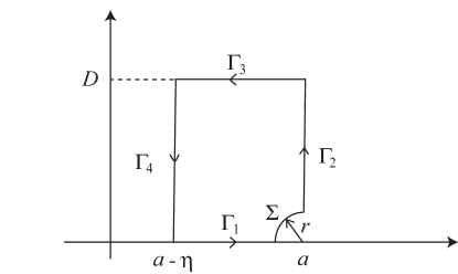
Figure 1. Contour $\Gamma$.

For $z\in\Gamma_{3}$, we write $z=u+iD$. Since $\overline{\zeta}(a,R)$ is real, a simple estimation gives

(4.36) $$|F_{R}(z)|\leq\frac{1}{D}e^{-\textup{Im}\;\overline{\zeta}(z,R)},\qquad\qquad z\in\Gamma_{3}.$$

From (4.31), it is readily seen that $\lim_{R\to\infty}\textup{Im}\;\overline{\zeta}(z,R)=+\infty$ uniformly for $z\in\Gamma_{3}$. Hence, $\lim_{R\to\infty}e^{-\textup{Im}\;\overline{\zeta}(z,R)}=0$ uniformly for $z\in\Gamma_{3}$. From (4.36), it follows that

(4.37) $$\lim_{R\to\infty}\int_{\Gamma_{3}}F_{R}(z)dz=0.$$

For $z\in\Gamma_{4}$, we write $z=a-\eta+iv$. Clearly

(4.38) $$|F_{R}(z)|\leq\frac{1}{\eta}e^{-\textup{Im}\;\overline{\zeta}(z,R)},\qquad\qquad z\in\Gamma_{4}.$$

Let $\sigma_{1}>0$ be any small number. From (4.31), we have $\lim_{R\to\infty}\textup{Im}\;\overline{\zeta}(z,R)=+\infty$ uniformly for $z\in\Gamma_{4}$ and $\textup{Im}\;z=v\geq\sigma_{1}$. Thus, $\lim_{R\to\infty}e^{-\textup{Im}\;\overline{\zeta}(z,R)}=0$ uniformly for $z\in\Gamma_{4}\cap\{z:\textup{Im}\;z\geq\sigma_{1}\}$ and

$$\lim_{R\to\infty}\int_{\Gamma_{4}}e^{-\textup{Im}\;\overline{\zeta}(z,R)}dz=\lim_{R\to\infty}\int^{a-\eta+i\sigma_{1}}_{a-\eta}e^{-\textup{Im}\;\overline{\zeta}(z,R)}dz.$$

From (4.31), it also follows that there is a constant $M_{5}>0$ such that $e^{-\textup{Im}\;\overline{\zeta}(z,R)}\leq M_{5}$. Hence

$$\biggl{|}\lim_{R\to\infty}\int_{\Gamma_{4}}e^{-\textup{Im}\;\overline{\zeta}(z,R)}dz\biggr{|}\leq M_{5}\sigma_{1}.$$

Since $\sigma_{1}$ can be arbitrarily small, we obtain

(4.39) $$\lim_{R\to\infty}\int_{\Gamma_{4}}e^{-\textup{Im}\;\overline{\zeta}(z,R)}dz=0.$$

Coupling (4.38) and (4.39) gives

(4.40) $$\lim_{R\to\infty}\int_{\Gamma_{4}}F_{R}(z)dz=0.$$

In a similar manner, one can establish

(4.41) $$\lim_{R\to\infty}\int_{\Gamma_{2}}F_{R}(z)dz=0.$$

By a combination of (4.34), (4.35), (4.37) and $(4.40)-(4.41)$, we obtain

(4.42) $$\begin{split}\lim_{R\to\infty}\int^{a}_{a-\eta}&\frac{\sin\{\overline{\zeta}(x,R)-\overline{\zeta}(a,R)\}}{\pi(x-a)}dx\\ &\hskip 46.09344pt=-\frac{1}{\pi}\textup{Im}\;\biggl{\{}\lim_{R\to\infty}\lim_{r\to 0^{+}}\int_{\Sigma}F_{R}(z)dz\biggr{\}}=\frac{1}{2}.\end{split}$$

Using (4.42), we are now ready to handle the limit on the right-hand side of the equation following (4.30).

For simplicity, let us write $\theta(x)=\theta(x,l)$; cf. (4.31). By the mean-value theorem, $\cos[\theta(x)-\theta(a)]=1+O\{(x-a)^{2}\}$ for $x$ near $a$. Hence, by the generalized Riemann-Lebesgue lemma, we have from (4.42)

(4.43) $$\lim_{R\to\infty}\int^{a}_{a-\eta}\frac{\sin\{\overline{\zeta}(x,R)-\overline{\zeta}(a,R)\}\cos[\theta(x)-\theta(a)]}{\pi(x-a)}dx=\frac{1}{2},$$

and also from (4.23) and (4.24)

(4.44) $$\lim_{R\to\infty}\int^{a}_{a-\eta}\frac{\cos\{\overline{\zeta}(x,R)-\overline{\zeta}(a,R)\}\sin[\theta(x)-\theta(a)]}{\pi(x-a)}dx=0.$$

Upon using an addition formula, it follows from (4.43) and (4.44) that

(4.45) $$\lim_{R\to\infty}\int^{a}_{a-\eta}\frac{\sin\{\zeta(x,l;R)-\zeta(a,l;R)\}}{\pi(x-a)}dx=\frac{1}{2}.$$

Coupling (4.30) and (4.45), we obtain

(4.46) $$\lim_{R\to\infty}\int^{a}_{a-\eta}\frac{\sin\{\zeta(x,l;R)-\zeta(a,l;R)\}}{\pi(x-a)}\phi(x)dx=\frac{1}{2}\phi(a^{-}).$$

In a similar manner, we also have

(4.47) $$\lim_{R\to\infty}\int_{a}^{a+\eta}\frac{\sin\{\zeta(x,l;R)-\zeta(a,l;R)\}}{\pi(x-a)}\phi(x)dx=\frac{1}{2}\phi(a^{+}).$$

A combination of (4.29), (4.46) and (4.47) yields

(4.48) $$\lim_{R\to\infty}\int^{c}_{d}\delta_{R}(x,a)\phi(x)dx=\frac{1}{2}[\phi(a^{-})+\phi(a^{+})].$$

Since $\varepsilon$ in (4.10) and (4.11) can be arbitrarily small, (4.8) now follows from (4.48). This completes the proof of the theorem. ∎

5. Airy and parabolic cylinder functions

We now turn our attention to the integral representation (1.7). Here, the interval of concern is the whole real line. However, the argument for this result remains similar to that for Theorems 1 & 2, and we will keep it brief. As before, we let $b$ and $\eta$ be positive numbers such that $b>\max\{1,|a|\}$. The Airy function $\textup{Ai}(t-x)$ is a solution of the equation

(5.1) $$\frac{d^{2}y}{dt^{2}}+(x-t)y=0,\qquad\qquad-\infty<t<\infty,$$

and satisfies

(5.2) $$\textup{Ai}(\infty)=\textup{Ai}^{\prime}(\infty)=0,$$

(5.3) $$\textup{Ai}(-t-x)=\frac{1}{\sqrt{\pi}}(t+x)^{-1/4}[\sin\zeta(x,t)+\varepsilon_{1}(x,t)],$$

and

(5.4) $$\textup{Ai}^{\prime}(-t-x)=-\frac{1}{\sqrt{\pi}}(x+t)^{1/4}[\cos\zeta(x,t)+\varepsilon_{2}(x,t)],$$

where $\varepsilon_{1}(x,t)=O(t^{-3/2})$ and $\varepsilon_{2}(x,t)=O(t^{-3/2})$, as $t\to\infty$, uniformly for $x>-b$, and where

(5.5) $$\zeta(x,t)=\frac{2}{3}(t+x)^{3/2}+\frac{\pi}{4}.$$

Define

(5.6) $$\delta_{R}(x,a)=\int^{\infty}_{-R}\textup{Ai}(t-x)\textup{Ai}(t-a)dt.$$

From (5.2), we have

(5.7) $$\delta_{R}(x,a)=\frac{\textup{Ai}(-R-x)\textup{Ai}^{\prime}(-R-a)-\textup{Ai}(-R-a)\textup{Ai}^{\prime}(-R-x)}{x-a};$$

see (3.6).

Theorem 3.

For any $a\in\mathbb{R}$ and any piecewise continuously differentiable function $\phi(x)$ on $(-\infty,\infty)$, we have

(5.8) $$\lim_{R\to\infty}\int^{\infty}_{-\infty}\phi(x)\int^{\infty}_{-R}\textup{Ai}(t-x)\textup{Ai}(t-a)dt\,dx=\frac{1}{2}[\phi(a^{-})+\phi(a^{+})],$$

provided that the two integrals

(5.9) $$\int^{-1}_{-\infty}|x|^{-\frac{3}{4}}|\phi(x)|dx\qquad and\qquad\int^{\infty}_{1}x^{-\frac{3}{4}}|\phi(x)|dx$$

are convergent.

Proof.

Using the asymptotic formulas (5.3) and (5.4), one can show from (5.7) that there are positive constants $M_{1}$ and $M_{2}$ such that

$$\int^{\infty}_{b}|\delta_{R}(x,a)\phi(x)|dx\leq M_{1}\int^{\infty}_{b}x^{-\frac{3}{4}}|\phi(x)|dx$$

and

$$\int^{-b}_{-\infty}|\delta_{R}(x,a)\phi(x)|dx\leq M_{2}\int_{-\infty}^{-b}|x|^{-\frac{3}{4}}|\phi(x)|dx$$

for $R>2|a|+1$. On account of the convergence of the two integrals in (5.9), for any $\varepsilon>0$ there is a constant $c>b$ such that

(5.10) $$\biggl{(}\int^{-c}_{-\infty}+\int^{\infty}_{c}\biggr{)}|\delta_{R}(x,a)\phi(x)|dx<\varepsilon$$

for all $R>2|a|+1$.

In view of the asymptotic formulas (5.3) and (5.4), equation (5.7) also gives

(5.11) $$\begin{split}\pi(x-a)\delta_{R}(x,a)=&\biggl{(}\frac{R+a}{R+x}\biggr{)}^{\frac{1}{4}}\sin\zeta(x,R)\cos\zeta(a,R)\\ &-\biggl{(}\frac{R+x}{R+a}\biggr{)}^{\frac{1}{4}}\cos\zeta(x,R)\sin\zeta(a,R)+\varepsilon(x,a;R),\end{split}$$

where $\varepsilon(x,a;R)=O(R^{-5/4})$, as $R\to\infty$, uniformly for $x,a\in(-b,b)$. In a manner similar to (4.29), by using the generalized Riemann-Lebesgue lemma we have

(5.12) $$\lim_{R\to\infty}\int^{c}_{-c}\delta_{R}(x,a)\phi(x)dx=\lim_{R\to\infty}\int^{a+\eta}_{a-\eta}\frac{\sin\{\zeta(x,R)-\zeta(a,R)\}}{\pi(x-a)}\phi(x)dx,$$

for any piecewise continuously differentiable function $\phi(x)$ and any $\eta>0$. Since $\zeta(x,R)-\zeta(a,R)=\sqrt{R}(x-a)+O(1/\sqrt{R})$ for large $R$ and bounded $x$ and $a$, we also have $\sin\{\zeta(x,R)-\zeta(a,R)\}=\sin(\sqrt{R}(x-a))+O(1/\sqrt{R})$ as $R\to\infty$ for bounded $x$ and $a$. Thus, equation (5.12) gives

(5.13) $$\lim_{R\to\infty}\int^{c}_{-c}\delta_{R}(x,a)\phi(x)dx=\lim_{R\to\infty}\int^{a+\eta}_{a-\eta}\frac{\sin\sqrt{R}(x-a)}{\pi(x-a)}\phi(x)dx.$$

By Jordan’s theorem on the Dirichlet kernel [2, p.473], the value of the last limit is $[\phi(a^{-})+\phi(a^{+})]/2$. The final result (5.8) now follows from (5.10) and (5.13). ∎

The parabolic cylinder function $W(a,x)$ is a solution of Weber’s equation

(5.14) $$\frac{d^{2}y}{dx^{2}}+\biggl{(}\frac{1}{4}x^{2}-a\biggr{)}y=0$$

with boundary conditions

(5.15) $$y(x)=\sqrt{\frac{2k_{a}}{x}}\biggl{[}\cos\zeta(a,x)+O\biggl{(}\frac{1}{x}\biggr{)}\biggr{]},\qquad\qquad x\to\infty,$$

and

(5.16) $$y(-x)=\sqrt{\frac{2}{k_{a}x}}\biggl{[}\sin\zeta(a,x)+O\biggl{(}\frac{1}{x}\biggr{)}\biggr{]},\qquad\qquad x\to\infty,$$

where $k_{a}=\sqrt{1+e^{2\pi a}}-e^{\pi a}$ and

(5.17) $$\zeta(a,x)=\frac{1}{4}x^{2}-a\ln x+\frac{1}{2}\arg\Gamma\biggl{(}\frac{1}{2}+ia\biggr{)}+\frac{\pi}{4};$$

see [1, p.693]. The derivative of this function has the behavior

(5.18) $$W^{\prime}(a,x)=-\sqrt{\frac{k_{a}x}{2}}\biggl{[}\sin\zeta(a,x)+O\biggl{(}\frac{1}{x}\biggr{)}\biggr{]},\qquad\qquad x\to\infty,$$

and

(5.19) $$W^{\prime}(a,-x)=-\sqrt{\frac{x}{2k_{a}}}\biggl{[}\cos\zeta(a,x)+O\biggl{(}\frac{1}{x}\biggr{)}\biggr{]},\qquad\qquad x\to\infty.$$

This function is also related to the parabolic cylinder function $U(a,x)$ via the connection formulas [1, p.693]

(5.20) $$W(a,x)=(2k_{a})^{\frac{1}{2}}e^{\frac{1}{4}\pi a}\,\textup{Re}\;\bigl{\{}e^{i(\frac{1}{2}\phi_{2}+\frac{1}{8}\pi)}U(ia,xe^{-\frac{1}{4}\pi i})\bigr{\}},$$

(5.21) $$W(a,-x)=(2/k_{a})^{\frac{1}{2}}e^{\frac{1}{4}\pi a}\,\textup{Im}\;\bigl{\{}e^{i(\frac{1}{2}\phi_{2}+\frac{1}{8}\pi)}U(ia,xe^{-\frac{1}{4}\pi i})\bigr{\}},$$

where $x>0$ and $\phi_{2}=\arg\Gamma(\frac{1}{2}+ia)$. From the integral representation [12, p.208]

(5.22) $$U(a,z)=\frac{e^{-\frac{1}{4}z^{2}}}{\Gamma(\frac{1}{2}+a)}\int^{\infty}_{0}e^{-zs-\frac{1}{2}s^{2}}s^{a-\frac{1}{2}}\,ds,\qquad\qquad\textup{Re}\;a>-\frac{1}{2},$$

one can easily show that

$$|U(ia,xe^{-\frac{1}{4}\pi i})|\leq\frac{2^{\frac{1}{4}}\sqrt{\pi}}{|\Gamma(\frac{1}{2}+ia)|}x^{-\frac{1}{2}}.$$

Since

$$\left|\Gamma({\textstyle\frac{1}{2}}+ia)\right|=\frac{\sqrt{\pi}}{(\cosh\pi a)^{1/2}}\sim\sqrt{2\pi}e^{-\frac{1}{2}\pi a}$$

and

$$\sqrt{2k_{a}}\sim e^{-\frac{1}{2}\pi a},\qquad\qquad\sqrt{\frac{2}{k_{a}}}\sim 2e^{\frac{1}{2}\pi a}$$

as $a\to+\infty$, it follows that for large positive $a$, there is a constant $M_{1}$ such that

$$\begin{split}&|W(a,x)|\leq M_{1}e^{\frac{1}{4}\pi a}x^{-\frac{1}{2}},\qquad\qquad x>0,\\ &|W(a,-x)|\leq M_{1}e^{\frac{5}{4}\pi a}x^{-\frac{1}{2}},\qquad\qquad x>0.\end{split}$$

As $a\to-\infty$, we have

$$\left|\Gamma({\textstyle\frac{1}{2}}+ia)\right|\sim\sqrt{2\pi}e^{\frac{1}{2}\pi a}=\sqrt{2\pi}e^{-\frac{1}{2}\pi|a|}$$

and

$$\sqrt{2k_{a}}\sim\sqrt{2},\qquad\qquad\sqrt{\frac{2}{k_{a}}}\sim\sqrt{2}.$$

Hence, there exists a constant $M^{\prime}_{1}>0$ such that for large negative $a$,

$$\begin{split}&|W(a,x)|\leq M^{\prime}_{1}e^{\frac{1}{4}\pi|a|}x^{-\frac{1}{2}},\qquad\qquad x>0,\\ &|W(a,-x)|\leq M^{\prime}_{1}e^{\frac{1}{4}\pi|a|}x^{-\frac{1}{2}},\qquad\qquad x>0.\end{split}$$

By using (5.20), (5.21) and (5.22), it can also be shown that there are positive constants $M_{2}$ and $M^{\prime}_{2}$ such that for large positive $a$,

$$\begin{split}&|W^{\prime}(a,x)|\leq M_{2}e^{\frac{1}{4}\pi a}x^{\frac{1}{2}},\qquad\qquad x>0,\\ &|W^{\prime}(a,-x)|\leq M_{2}e^{\frac{5}{4}\pi a}x^{\frac{1}{2}},\qquad\qquad x>0,\end{split}$$

and for large negative $a$,

$$\begin{split}&|W^{\prime}(a,x)|\leq M^{\prime}_{2}e^{\frac{1}{4}\pi|a|}x^{\frac{1}{2}},\qquad\qquad x>0,\\ &|W^{\prime}(a,-x)|\leq M^{\prime}_{2}e^{\frac{1}{4}\pi|a|}x^{\frac{1}{2}},\qquad\qquad x>0.\end{split}$$

We define

(5.23) $$\delta_{R}(a,b)=\int^{R}_{-R}W(a,x)W(b,x)dx.$$

From (5.14), one can derive

$$\delta_{R}(a,b)=\frac{W(a,x)W^{\prime}(b,x)-W^{\prime}(a,x)W(b,x)}{b-a}\biggl{|}^{R}_{-R}.$$

Using the asymptotic formulas (5.15) and (5.18), we obtain

$$(b-a)\delta_{R}(a,b)=\biggl{(}\sqrt{k_{a}k_{b}}+\frac{1}{\sqrt{k_{a}k_{b}}}\biggl{)}\sin\{\zeta(a,R)-\zeta(b,R)\}+O\biggl{(}\frac{1}{R}\biggr{)}.$$

By an argument similar to that for Theorem 3, one can establish the following result.

Theorem 4.

For any $a\in\mathbb{R}$ and any piecewise continuously differentiable function $\phi(x)$ on $(-\infty,+\infty)$, we have

$$\lim_{R\to\infty}\int^{+\infty}_{-\infty}\phi(b)\int^{R}_{-R}W(a,x)W(b,x)\,dx\,db=\pi\sqrt{1+e^{2\pi a}}[\phi(a^{-})+\phi(a^{+})],$$

provided that two integrals

$$\int^{-1}_{-\infty}|\phi(x)|e^{\frac{1}{4}\pi|x|}\frac{dx}{|x|}\qquad and\qquad\int^{\infty}_{1}|\phi(x)|e^{\frac{5}{4}\pi x}\frac{dx}{x}$$

are convergent.

6. Series representations

To prove the representations in $(1.8)-(1.11)$, we only need to recall some expansion theorems concerning orthogonal polynomials (functions). For instance, in the case of Legendre polynomials $P_{n}(x)$, Theorem 1 in [9, p.55] can be stated in the following form.

Theorem 5.

Let $f(x)$ be a piecewise continuously differentiable function in $(-1,1)$, and put

(6.1) $$\delta_{n}(t,x)=\sum^{n}_{k=0}\biggl{(}k+\frac{1}{2}\biggr{)}P_{k}(t)P_{k}(x).$$

If the integral

$$\int^{1}_{-1}f^{2}(x)\,dx$$

is finite, then

(6.2) $$\lim_{n\to\infty}\int^{1}_{-1}\delta_{n}(t,x)f(t)\,dt=\frac{1}{2}[f(x^{+})+f(x^{-})].$$

The statement in (6.2) is equivalent to that in (1.8); i.e., the finite sum in (6.1) defines a delta sequence. In a similar manner, one can restate Theorems 2 and 3 in [9, p.71 and p.88] as follows.

Theorem 6.

Let $f(x)$ be a piecewise continuously differentiable function in $(-\infty,\infty)$, and put

(6.3) $$\delta_{n}(t,x)=e^{-t^{2}}\sum^{n}_{k=0}\frac{1}{2^{k}k!\sqrt{\pi}}H_{k}(t)H_{k}(x).$$

If the integral

$$\int^{\infty}_{-\infty}e^{-x^{2}}f^{2}(x)\,dx$$

is finite, then

(6.4) $$\lim_{n\to\infty}\int^{\infty}_{-\infty}\delta_{n}(t,x)f(t)\,dt=\frac{1}{2}[f(x^{+})+f(x^{-})].$$

Theorem 7.

Let $f(x)$ be a piecewise continuously differentiable function in $(0,\infty)$, and put

(6.5) $$\delta_{n}(t,x)=e^{-t}t^{\alpha}\sum^{n}_{k=0}\frac{k!}{\Gamma(k+\alpha+1)}L^{(\alpha)}_{k}(t)L^{(\alpha)}_{k}(x).$$

If the integral

$$\int^{\infty}_{0}e^{-t}t^{\alpha}f^{2}(t)\,dt,\qquad\qquad\alpha>-1,$$

is finite, then

(6.6) $$\lim_{n\to\infty}\int^{\infty}_{0}\delta_{n}(t,x)f(t)\,dt=\frac{1}{2}[f(x^{+})+f(x^{-})].$$

To demonstrate (1.11), we recall the Laplace series expansion

(6.7) $$f(\theta_{1},\phi_{1})=\sum^{\infty}_{k=0}\frac{2k+1}{4\pi}\int^{\pi}_{-\pi}\int^{\pi}_{0}f(\theta_{2},\phi_{2})P_{k}(\cos\gamma)\sin\theta_{2}d\theta_{2}d\phi_{2},$$

where $\cos\gamma=\cos\theta_{1}\cos\theta_{2}-\sin\theta_{1}\sin\theta_{2}\cos(\phi_{1}-\phi_{2})$ and $P_{k}(x)$ is a Legendre polynomial; see [6, p.147]. By the addition formula [3, p.797]

(6.8) $$P_{k}(\cos\gamma)=\frac{4\pi}{2k+1}\sum^{k}_{l=-k}Y_{kl}(\theta_{1},\phi_{1})Y^{*}_{kl}(\theta_{2},\phi_{2}),$$

we can rewrite (6.7) in the form

(6.9) $$f(\theta_{1},\phi_{1})=\sum^{\infty}_{k=0}\int^{\pi}_{-\pi}\int^{\pi}_{0}f(\theta_{2},\phi_{2})\sin\theta_{2}\sum^{k}_{l=-k}Y_{kl}(\theta_{1},\phi_{1})Y^{*}_{kl}(\theta_{2},\phi_{2})d\theta_{2}d\phi_{2}.$$

For $f\in C([0,\pi]\times[-\pi,\pi])$, the series on the right converges pointwise to the function on the left; see [6, p.344]. This result can be expressed as follows.

Theorem 8.

Let $f(\theta_{1},\phi_{1})$ be a continuous function on $[0,\pi]\times[-\pi,\pi]$, and put

(6.10) $$\delta_{n}(\theta_{1},\theta_{2})\delta_{n}(\phi_{1},\phi_{2}):=\sin\theta_{2}\sum^{n}_{k=0}\sum^{k}_{l=-k}Y_{kl}(\theta,\phi_{1})Y^{*}_{kl}(\theta_{2},\phi_{2}).$$

Then, we have

(6.11) $$f(\theta_{1},\phi_{1})=\lim_{n\to\infty}\int^{\pi}_{-\pi}\int^{\pi}_{0}\delta_{n}(\theta_{1},\theta_{2})\delta_{n}(\phi_{1},\phi_{2})f(\theta_{2},\phi_{2})\,d\theta_{2}\,d\phi_{2}.$$

Equation (6.11) is equivalent to saying that $\delta_{n}(\theta_{1},\theta_{2})\delta_{n}(\phi_{1},\phi_{2})$ is a delta sequence of $\delta(\theta_{1}-\theta_{2})\delta(\phi_{1}-\phi_{2})$ for $\theta_{1},\theta_{2}\in[0,\pi]$ and $\phi_{1},\phi_{2}\in[-\pi,\pi]$. The use of the identity $\delta(\cos\theta_{1},\cos\theta_{2})=\frac{1}{\sin\theta_{2}}\delta(\theta_{1}-\theta_{2})$ gives (1.11); see [8, p.49].

References

- [1] (0167642) M. Abramowitz and I. A. Stegun (eds.), “Handbook of Mathematical Functions,” Appl. Math. Ser. No. 55, National Bureau of Standards, Washington, D.C., 1964. (Reprinted by Dover, New York, 1965).
- [2] (0087718) T. M. Apostol, “Mathematical Analysis,” Addison-Wesley, Reading, MA, 1957.
- [3] (1810939) G. B. Arfken and H. J. Weber, “Mathematical Methods for Physicists (6th ed.),” Elsevier, Oxford, 2005.
- [4] (0240343) H. Buchholz, “The Confluent Hypergeometric Function,” Springer-Verlag, Berlin and New York, 1969.
- [5] (0166596) I. M. Gel’fand and G. E. Shilov, “Generalized Functions,” Academic Press, New York and London, 1964.
- [6] (0064922) E. W. Hobson, “The Theory of Spherical and Ellipsoidal Harmonics (2nd ed.),” Chelsea Publishing Co., New York, 1955.
- [7] (0217534) D. S. Jones, “Generalized Functions,” McGraw-Hill, London, 1966.
- [8] (1604296) R. P. Kanwal, “Generalized Functions: Theory and Techniques (2nd ed.),” Birkhäuser, Boston, 1998.
- [9] (0174795) N. N. Lebedev, “Special Functions and Their Applications,” Prentice-Hall, London, 1965.
- [10] (0092119) M. J. Lighthill, “Introduction to Fourier Analysis and Generalized Functions,” Cambridge University Press, Cambridge, 1958.
- [11] (0059774) P. M. Morse and H. Feshbach, “Methods of Theoretical Physics,” Vol. 1, McGraw-Hill, New York, 1953.
- [12] (1429619) F. W. J. Olver, “Asymptotics and Special Functions,” A. K. Peters, Wellesley, MA, 1997. (Reprinted, with corrections, of original Academic Press edition, 1974).
- [13] F. W. J. Olver, D. W. Lozier, C. W. Clark and R. F. Boisvert (eds.), “NIST Handbook of Mathematical Functions,” National Institute of Standards and Technology, Gaithersburg, Maryland, to appear.
- [14] (0365062) W. Rudin, “Functional Analysis,” McGraw-Hill, New York, 1973.
- [15] (0207494) L. Schwartz, “Mathematics for the Physical Sciences,” Addison-Wesley, Reading, MA, 1966.
- [16] (1911183) M. J. Seaton, Coulomb functions for attractive and repulsive potentials and for positive and negative energies, Comput. Phys. Comm., 146 (2002), 225–249.
- [17] (2114198) O. Vallée and M. Soares, “Airy Functions and Applications to Physics,” Imperial College Press, London, distributed by World Scientific, Singapore, 2004.