Techniques for targeted Fermi-GBM follow-up of gravitational-wave events

Abstract

The Advanced LIGO and Advanced Virgo ground-based gravitational-wave (GW) detectors are projected to come online 2015–2016, reaching a final sensitivity sufficient to observe dozens of binary neutron star mergers per year by 2018. We present a fully-automated, targeted search strategy for prompt gamma-ray counterparts in offline Fermi-GBM data. The multi-detector method makes use of a detailed model response of the instrument, and benefits from time and sky location information derived from the gravitational-wave signal.

I Introduction

Compact binary coalescence (CBC), such as the merger of two neutron stars (NS) or black holes (BH), remains the most highly anticipated gravitational-wave signal for ground-based gravitational-wave detectors. The second-generation Advanced LIGO (4km-baseline interferometers in Hanford, WA and Livingston, LA) (Harry, 2010) and Advanced Virgo (3km interferometer in Cascina, Italy) (Accadia et al., 2012) detectors are projected to come online 2015–2016, and reach a final sensitivity sufficient to observe dozens of NS-NS mergers per year by 2018. Together with the 600m GEO-HF detector (Willke et al., 2006), they will form a word-wide network of gravitational-wave interferometric detectors. The network will be joined by the Japanese 3km cryogenic KAGRA detector (Somiya, 2012) and a proposed third LIGO-India detector around 2018–2020, increasing overall sensitivity and sky-coverage, while also improving sky localization and waveform reconstruction (Schutz, 2011).

Gravitational-waves have yet to be directly observed. Our confidence in the existence of compact binary coalescence events comes primarily from the discovery of a small number of galactic pulsars which appear to be in close binary systems with another neutron star. The first and most famous of these systems contains the Hulse-Taylor pulsar PSR B1316+16. It has demonstrated over many decades an orbital decay consistent with loss of energy to gravitational waves (Weisberg et al., 2010). The number and inferred lifetime of these systems can be used to obtain an estimate of about one NS-NS merger event per Mpc³ per million years (Abadie et al., 2010a), with up to two orders of magnitude uncertainty in rate due largely to our limited knowledge of the pulsar luminosity function and limited statistics. The merger rate translates into an estimate of $\sim$0.02 detectable NS-NS merger events per year for the initial LIGO-Virgo detector network, which operated between 2005–2010, and $\sim$40 per year for the advanced detectors once they reach design sensitivity. Although their gravitational radiation is stronger, the merger rates of NS-BH binaries is more uncertain as we have not observed any NS-BH binary systems, and have generally poor knowledge of the black hole mass distribution.

Gamma-ray bursts (GRB) are flashes of gamma rays observed approximately once per day. Their isotropic distribution in the sky was the first evidence of an extra-galactic origin, and indicated that they were extremely energetic events. The duration of prompt gamma-ray emission shows a bi-modal distribution which naturally groups GRBs into two categories (Kouveliotou et al., 1993). Most long GRBs emit their prompt radiation over timescales $\gtrsim$2 seconds, and as much as hundreds of seconds. They have been associated with young stellar populations and the collapse of rapidly rotating massive stars (Hjorth and Bloom, 2011). Short GRBs (sGRB), with prompt emission typically less than 1s and a generally harder spectrum, are found in both old and new stellar populations. Mergers of two neutron stars, or of neutron star/black hole systems, are thought thought to be a major contribution to the sGRB population (Nakar, 2007). It is this favored progenitor model which makes short GRBs and associated afterglow emission a promising counterpart to gravitational-wave observations.

Since 2005, the Swift satellite has revolutionized our understanding of short GRBs by the rapid observation of x-ray afterglows, providing the first localization, host identification, and red-shift information (Gehrels et al., 2009). The beaming angle for short GRBs is highly uncertain, although limited observations of jet breaks in some afterglows imply half-opening angles of $\theta_{j}\sim$ 3–14 degrees (Liang et al., 2008; Fong et al., 2012). The absence of an observable jet break sets a lower limit on the opening angle which is generally weak (due to limits in sensitivity), though in the case of GRB 050724A, late-time Chandra observations were able to constrain $\theta_{j}\gtrsim 25^{\circ}$  (Grupe et al., 2006).

The observed spatial density of sGRB’s and limits on beaming angle result in a NS-NS merger event rate roughly consistent with that derived from galactic binary pulsar measurements. Although the beaming factor of $\sim\theta_{j}^{2}/2$ means we believe most merger events seen by the advanced GW detectors will not be accompanied by a standard gamma-ray burst, this is somewhat compensated by the fact that the ones that are beamed toward us have stronger gravitational-wave emission. Current estimates for coincident GW-sGRB observation for advanced LIGO-Virgo are a few per year assuming a NS-NS progenitor model (Metzger and Berger, 2012; Coward et al., 2012). The rate increases by a factor of 8 if all observed short GRBs are instead due to NS-BH (10 $M_{\odot}$) mergers which are detectable in gravitational-waves to about twice the distance.

In addition to the jet-driven burst and afterglow, other EM emission associated with a compact merger can be a promising channel for GW-EM coincidence, particularly if the EM radiation is less-beamed or even isotropic. A few short GRBs ($\sim$10%) have shown clear evidence of high-energy flares which precede the primary burst by 1–10 seconds, and possibly up to 100s (Troja et al., 2010). The precursors can be interpreted as evidence of some activity during or before merger, such as the resonant shattering of NS crusts (Tsang et al., 2012), which could radiate isotropically. Thus it will be interesting to search for weak non-standard EM emission accompanying all nearby NS-NS mergers seen in GWs, while we expect only a small fraction to be oriented in our line-of-sight for a standard jet-driven sGRB.

The Gamma-ray Burst Monitor (GBM) (Meegan et al., 2009) aboard the Fermi spacecraft measures photon rates from 8 keV–40 MeV. The instrument consists of 12 semi-directional NaI scintillation detectors and 2 BGO scintillation detectors which cover the entire sky not occluded by the Earth (about 65%). The lower-energy NaI detectors have an approximately $\cos{\theta}$ response relative to angle of incidence, and relative rates across detectors are used to reconstruct the source location to a few degrees. The BGO detectors are much less directional, and are used to detect and resolve the higher energy spectrum above $\sim$200 MeV.

GBM produces on-board triggers for gamma-ray burst events by looking for multi-detector rate excess over background across various energy bands and timescales. In the case of a trigger, individual photon information is sent to the ground and the event is publicly reported. Those events which have been confirmed as GRBs have already been studied in coincidence with LIGO-Virgo data (Abbott et al., 2010; Abadie et al., 2010b, 2012a). So far, no gravitational-wave counterparts to triggered GRBs have been identified, which was not unexpected given the limited reach of the first generation instruments.

In addition to the triggered events, survey data is available which records binned photon counts over all time. In this proposed offline analysis of short transients, we consider the CTIME daily data, which contains counts binned at 0.256s over 8 energy channels for each detector. A new GBM data product (continuous TTE) was implemented in late 2012. It provides continuous data on individual photons with 2$\mu$s and 128 energy channel resolution, which will further enhance offline sensitivity to particularly short bursts.

This paper discusses the possibility of using these offline GBM data products to follow-up gravitational-wave candidates in the advanced LIGO-Virgo era. In section II we describe the characteristics of a trigger provided by gravitational-wave data. Sections III and IV develop a likelihood-ratio based procedure for analyzing available GBM offline data about the time and sky location provided by the gravitational waves. Finally, in section V we demonstrate the performance of the search algorithm on background times and a sample of known sGRB’s.

II Gravitational-wave trigger

Searches for NS-NS and NS-BH coalescence in gravitational-wave data typically use matched filtering of the model waveform (Abadie et al., 2012b; Abadie et al., 2012c). The gravitational waves from CBC are characterized by a chirp of monotonically increasing frequency and amplitude as the binary inspirals under approximately adiabatic orbital decay. During this progression, kilometer-scale interferometers are sensitive to the inspiral phase of a stellar-mass coalescence until just prior to merger, but before any tidal effects on a NS become important.

The waveform in this regime is well-modeled using post-Newtonian techniques, and can be considered a standard candle encoding orbital parameters of the system. Mass, spin, and coalescence time are accessible with the GW projection onto a single detector, while distance, inclination, and sky location degeneracies can be disentangled to varying degrees of success using coherent data from multiple detectors, for example by using Bayesian inference (Veitch et al., 2012). A typical gravitational-wave detection in the early advanced detector era may have moderate signal-to-noise $\sim$8 in two or more detectors, estimated merger time to within milliseconds, and sky localization to $\sim$100 square degrees depending on detector network configuration (Fairhurst, 2011). Figure 1 shows a reconstructed 3-detector localization for a simulated signal near detection threshold.

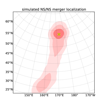
Figure 1: Example sky localization of simulated NS-NS merger seen in modeled gravitational-wave data with noise similar in spectrum to that expected from the advanced LIGO-Virgo GW network. The signal-to-noise of the GW signal in each detector is 8.7 (H1) 7.2 (L1) and 3.1 (V1), and the sky location is determined through Bayesian inference using a nested sampling technique (Veitch et al., 2012) applied to data from all detectors. The elongated shape beyond 1$\sigma$ is due to a small degenerate timing uncertainty in V1.

III Coherent analysis of GBM data

In this section, we develop a procedure to coherently search GBM detector data for modeled events. The basic idea is that by processing multiple detector data coherently, we can obtain a greater sensitivity than when considering one detector at a time. Greater computational resources available offline (vs. on-board) also allow for more careful background estimation to be done. For this analysis, we can relax to some extent the strict 2-detector coincidence requirement used to veto spurious events on-board as the gravitational-wave trigger means much less time and sky area is considered.

III.1 GBM background estimation

Each detector is subject to a substantial time-varying background from bright high-energy sources that come in and out of the wide field of view, as well as location-dependent particle and Earth atmospheric effects. This background must be estimated and subtracted out to look for any prompt excess. Methods in use include the local averaging of previous data done on-board, smooth spline-fits with a high-frequency cutoff, direct tracking and modeling of the dominant sources, and averaging rates from previous orbits with similar orientations (Finger et al., 2009; Wilson-Hodge et al., 2012; Fitzpatrick et al., 2012). In this analysis where we are interested in the background estimate for a short foreground interval [$-T/2$, $+T/2$] where $T\sim$1s, we estimate the background using a polynomial fit to local data from [$-10T$, $+10T$] (minimum $\pm 5s$), excluding time [$-3T/2$, $+5T/2$] around the foreground interval to avoid bias from an on-source excess. An example of the foreground and background intervals about a strong prompt signal is shown in figure 2. The polynomial degree is determined by the interval length to account for more complicated background variability over longer intervals. It ranges from 2 (minimum) to 1+$0.5\log_{2}T$. The quality of the fit is determined using a $\chi^{2}$ statistic applied to the data, re-binned at $T/4$ seconds for $T>1$s. If the $\chi^{2}$ per degree-of-freedom is over 2, or if any of the $N$ individual data points has $\chi^{2}>4\ln N$, it is assumed that the polynomial could not adequately model the local background variability, and the fit is redone over the smaller interval [$-5T$, $+5T$]. If the fit continues to fail the $\chi^{2}$ test at the looser requirements of 3 and $6\ln N$ respectively, the background estimate is marked unreliable and not used in further computations for that particular foreground interval.

High-energy cosmic rays striking a NaI crystal can result in long-lived phosphorescent light emission. The detector may interpret this is a rapid series of events, creating a short-lived jump in rates for one or multiple channels, and severely distorting the background fit if not accounted for. They are identified with a simple procedure that compares the counts in each 0.256s bin against the mean rate estimated from four neighboring bins. If an excess is detected to 5$\sigma$ or more, that measurement and the immediately neighboring bin on either side is removed from the background fit for all channels of the affected detector. A much stricter requirement is used when rejecting cosmic-ray events in the foreground interval. In that case, a 0.256s measurement must have signal-to-noise over $500/\sqrt{T}$ for it to be excised, which is much larger than expected for true GRBs.

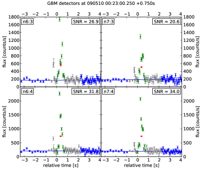
Figure 2: Detector and channel-dependent polynomial background fitting applied to GRB 090510A. Four of the 8 $\times$ 14 channel and detector combinations are shown. The green represents the highest likelihood foreground interval, and the background contribution is estimated using a polynomial fit to the region (cropped) shown in blue. Red dots mark the average flux in the foreground interval.

III.2 Likelihood-ratio statistic

A likelihood ratio combines information about sources and noise into a single variable. It is defined as the probability of measuring the observed data, $d$, in the presence of a particular true signal $H_{1}$ (source amplitude $s>0$) divided by the probability of measuring the observed data in noise alone $H_{0}$ ($s=0$).

$$\Lambda(d)=\frac{P(d|H_{1})}{P(d|H_{0})}$$ (1)

When signal parameters such as light-curve, spectrum, amplitude $s$ and sky-location $\alpha,\delta$ are unknown, one can either marginalize over the unknown parameters, or take the maximum likelihood over the range to obtain best-fit values.

For $i$ measurements of sufficiently binned, uncorrelated Gaussian data,

$$P(d_{i}|H_{1}) =\prod_{i}{\frac{1}{\sqrt{2\pi}\sigma_{d_{i}}}\exp\left(-\frac{(\tilde{d_{i}}-r_{i}s)^{2}}{2\sigma_{d_{i}}^{2}}\right)}$$ (2)

$$P(d_{i}|H_{0}) =\prod_{i}{\frac{1}{\sqrt{2\pi}\sigma_{n_{i}}}\exp\left(-\frac{\tilde{d_{i}}^{2}}{2\sigma_{n_{i}}^{2}}\right)}$$ (3)

where we have used $\tilde{d_{i}}=d_{i}-\langle n_{i}\rangle$ to represent the background-subtracted measurements (e.g. red dots minus blue curve in figure 2), $\sigma_{n_{i}}$ and $\sigma_{d_{i}}$ for the standard deviation of the background and expected data (background+signal), $r_{i}$ for the location/spectrum-dependent instrumental response, and $s$, a single intrinsic source amplitude scaling factor at the Earth. Maximizing the likelihood ratio is the same as maximizing the log-likelihood ratio $\mathcal{L}=\ln{\Lambda}$,

$$\mathcal{L}=\sum_{i}{\left[\ln{\frac{\sigma_{n_{i}}}{\sigma_{d_{i}}}}+\frac{\tilde{d_{i}}^{2}}{2\sigma_{n_{i}}^{2}}-\frac{(\tilde{d_{i}}-r_{i}s)^{2}}{2\sigma_{d_{i}}^{2}}\right]}$$ (4)

When the first two terms are fixed, maximizing the log-likelihood ratio is equivalent to minimizing the the third term which we recognize as a $\chi^{2}$ fit to the two free sky-location parameters in $r_{i}$ and the single amplitude parameter $s$. The shape of the likelihood function over source amplitude $s$ is the product of (almost) Gaussians centered about the best-estimate of $s$ in each measurement, and the total likelihood is scaled by the sum of the squared signal-to-noise of all measurements.

The dependence of response factors $r_{i}$ on sky location is complicated, so the likelihood ratio is calculated over a sample grid of all possible locations. Assuming a single location, the remaining free parameter is the source amplitude $s$. The variance in the background-subtracted detector data includes both background and source contributions,

$$\sigma_{d_{i}}^{2}=\sigma_{n_{i}}^{2}+r_{i}s+\sigma_{r_{i}}^{2}s^{2}\quad(s\geq 0)$$ (5)

with $\sigma_{r_{i}}^{2}$ representing Gaussian-modeled systematic uncertainty in the instrumental response. Source terms are only included for physical $s\geq 0$ else their contribution is zero. The background contributes Poisson error, as well as any systematic variance $\sigma_{b_{i}}^{2}$ from poor background fitting which is also assumed to be Gaussian,

$$\sigma_{n_{i}}^{2}=\langle n_{i}\rangle+\sigma_{b_{i}}^{2}.$$ (6)

We find $s_{\mathrm{best}}$ which maximizes $\mathcal{L}$ by setting the derivative $d\mathcal{L}/ds$ to zero. If $\sigma_{d_{i}}=\sigma_{n_{i}}$, which happens when $rs\ll\sigma_{n}^{2}$, $\sqrt{2\mathcal{L}_{\mathrm{max}}}$ reduces to a coherent SNR (sum data using weights $r_{i}/\sigma_{n_{i}}^{2}$). If $\sigma_{d_{i}}$ can be assumed constant, the solution for $s_{\mathrm{best}}$ is found analytically,

$$s_{\mathrm{best}}\approx\frac{\sum_{i}{r_{i}\tilde{d_{i}}/\sigma_{d_{i}}^{2}}}{\sum_{i}{r_{i}^{2}/\sigma_{d_{i}}^{2}}},$$ (7)

which is just an appropriately inverse-noise weighted sum of the individual estimates of $s$ from each measurement. Although $\sigma_{d_{i}}$ depends on $s$, we can make the practical approximation $\sigma_{d_{i}}^{2}\approx\max(\langle n_{i}\rangle,d_{i})+\sigma_{b_{i}}^{2}$ as an initial guess.

To find the true maximum, we solve for $d\mathcal{L}/ds=0$ using Newton’s method, beginning with the value of the first derivative at our initial guess $s_{0}$, and using the analytic second derivative to refine the measurement: $s_{\mathrm{best}}\approx s_{0}-(\partial\mathcal{L}/\partial s)/(\partial^{2}\mathcal{L}/\partial s^{2})$. This calculation is both fast and easily vectorized. One initial guess using equation 7 followed by a couple iterations of Newton’s method generally provides an excellent approximation for $s_{\mathrm{best}}$.

So far we have been calculating the probability of a signal assuming a specific source amplitude $s$. To consider all possible source amplitudes we need to integrate the likelihood $P(d|s)$ (equation 2) over a prior on $s$,

$$P(d)=\int{P(d|s)P(s)ds}$$ (8)

For a given set of detector data $d$, the likelihood $P(d|s)$ over $s$ is almost the product of individual Gaussian distributions (not quite Gaussian because $\sigma_{d}$ depends on $s$). The product of Gaussian distributions with mean values $\mu_{i}$ and standard deviations $\sigma_{i}$ is itself Gaussian with mean and variance,

$$\mu_{\mathrm{prod}}=\frac{\sum{\mu_{i}/\sigma^{2}_{i}}}{\sum{1/\sigma^{2}_{i}}},\quad\sigma^{2}_{\mathrm{prod}}=\frac{1}{\sum{1/\sigma^{2}_{i}}}$$ (9)

In this case, $\mu_{i}=\tilde{d_{i}}/r_{i}$ and $\sigma_{i}=\sigma_{d_{i}}/r_{i}$. The mean value $\mu_{\mathrm{prod}}$ is the same as our initial guess for $s$ at maximum likelihood (equation 7), but we can assume to have a more accurate maximum-likelihood location $s_{\mathrm{best}}$ from the numerical procedure outlined above. The estimate for the variance of $\mathcal{L}$ over $s$ is,

$$\sigma_{\!\mathcal{L}}^{2}=\frac{1}{\sum{r_{i}^{2}/\sigma_{d_{i}}^{2}}},\quad\sigma^{2}_{d_{i}}\text{ evaluated at }s_{\mathrm{best}}$$ (10)

For a flat prior $P(s)=1$, we can integrate equation 8 by simply considering the area of a Gaussian with peak value $P(d|s_{\mathrm{best}})$ and variance $\sigma_{\!\mathcal{L}}^{2}$. Other choices for a prior can be represented by a power-law distribution $P(s)\propto s^{-\beta}$. A spatially homogeneous population, suitable for nearby sources, would assume $\beta=5/2$, while the empirical distribution for observed GRB amplitudes follows a power-law decay closer to $\beta\approx 1.8$, reflecting cosmological effects. If instead we are looking for signals from a particular host galaxy at known location and distance, we want to use an intrinsic source luminosity distribution. A convenient option is to use a scale-free prior with fixed $\beta=1$, so that our choice of form for an amplitude prior at the Earth does not translate back into a luminosity distribution that varies with distance.

One difficulty with any power-law prior is that it diverges for $s\to 0$. In a reasonable scenario of SNR $>$a few, the integral over $s$ will consist of two distinct contributions. The first is a Gaussian component with $\mu=s_{\mathrm{best}}$ and variance $\sigma_{\!\mathcal{L}}^{2}$, scaled by the prior $P(s_{\mathrm{best}})$. The second component is an infinite contribution from the divergent prior at $s=0$ with little contribution afterward due to suppression from the Gaussian tail. The infinite contribution represents the certainty of a signal of arbitrarily small amplitude to be present in the data, regardless of the ability of the data to resolve it. For moderate SNR, it’s very easy to isolate only the Gaussian contribution by placing a small cut on amplitude, truncating the likelihood for $s<s_{\mathrm{cut}}$. Under the approximation that $P(s)$ varies slowly over the width of the Gaussian, the log-likelihood marginalized over all $s$ becomes,

$$\mathcal{L}(d)=-\beta\ln{s_{\mathrm{best}}}+\ln{\sigma_{\!\mathcal{L}}}+\mathcal{L}(d|s_{\mathrm{best}})$$ (11)

up to common additive constants that do not depend on the data $d$.

The approximation for the marginalized likelihood becomes problematic for small $s_{\mathrm{best}}$ where the assumption that $P(s)$ is constant over the range of the Gaussian breaks down, and the Gaussian distribution can no longer be isolated from the divergence at small $s$. We enforce a finite and well-behaved prior by multiplying by a prefactor,

$$P(s)=\left[1-e^{-\left(s/\gamma\sigma_{\!\mathcal{L}}\right)^{\beta}}\right]s^{-\beta}$$ (12)

so that $P(s)$ reaches a maximum constant value of $(1/\gamma\sigma_{\!\mathcal{L}})^{\beta}$ for small $s$. The tunable parameter $\gamma$ sets the number of standard deviations at which the prior begins to plateau, and we use $\gamma=2.5$. This allows us to use the approximation that $P(s)$ is reasonably constant over a range of $\sigma_{\!\mathcal{L}}$ for any $s>0$. The only remaining correction is to account for clipping of the Gaussian for non-physical $s<0$, which can be represented by the error function. The final approximation for the amplitude-marginalized log-likelihood becomes,

$$\mathcal{L}(d)=\ln\sigma_{\!\mathcal{L}}+\ln\left[1+\mathrm{Erf}\left(\frac{s_{\mathrm{best}}}{\sqrt{2}\sigma_{\!\mathcal{L}}}\right)\right]+\mathcal{L}(d|s_{\mathrm{best}})$$

$$+\left\{\begin{array}[]{ll}\ln\left[1-e^{-\left(s_{\mathrm{best}}/\gamma\sigma_{\!\mathcal{L}}\right)^{\beta}}\right]-\beta\ln{s_{\mathrm{best}}}&s_{\mathrm{best}}>0\\ -\beta\ln\left(\gamma\sigma_{\!\mathcal{L}}\right)&s_{\mathrm{best}}\leq 0\end{array}\right.$$ (15)

which contains factors form the Gaussian width, fractional overlap with $s>0$, maximum likelihood at $s_{\mathrm{best}}$, and scaling from $P(s)$ respectively. Finally we are free to calibrate the log-likelihood by subtracting the expected $\mathcal{L}(d)$ calculated for no signal at a reference sensitivity: $\mathcal{L}_{\mathrm{ref}}=-\beta\ln\gamma+(1-\beta)\ln\sigma_{\mathcal{L},\mathrm{ref}}$. $\sigma_{\!\mathcal{L}}$ represents the source amplitude required for a $1\sigma$ excess in the combined data, and is around 0.05 photons/s/cm${}^{2}\times(T/1$s$)^{-1/2}$ [50–300 keV] for typical source spectra and reference background levels. Figure 3 shows the coherent signal-to-noise expected from all detectors for a 0.512s-long event with normal GRB spectrum and constant amplitude of 1.0 photons/s/cm², and compares it to the SNR expected from the most favorably-oriented individual detector alone in the 50–300 keV band.

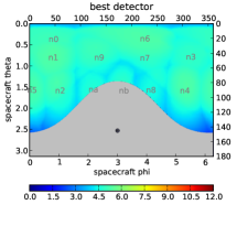
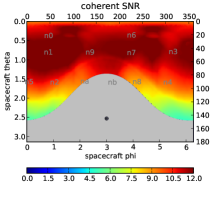
Figure 3: Signal-to-noise expected from GRBs with a normal spectrum, and coming from various positions across the GBM field-of-view. The hypothetical signal lasts 0.512s and is normalized to 1.0 photons/s/cm² in the 50–300 keV band, while background rates and Earth position are selected from 10 seconds prior to GRB 090305A. The instrumental response includes contributions from atmospheric scattering in the 50–300 keV band. The first map shows the signal-to-noise from the single best detector over 50–300 keV. The second plot shows the SNR expected from a coherent analysis of the full CTIME data. The coherent statistic must be calculated for all directions, which means it is subject to a trials factor equal to the number of independent sky locations.

IV Performing the follow-up

For a single gravitational-wave trigger, we search a standard sGRB accretion timescale of [0, 5s] relative to the time of coalescence for prompt flux excess in GBM between 0.256 and 2s long (the lower limit of 0.256s set by the CTIME archival resolution does not apply to continuous TTE data). We also search a prior interval [–30s, 0s] for possible precursor bursts between 0.256s and 2s. Finally we may include bursts between 2s to 32s in an extended interval [–30s, 300s] to search for possible longer-duration emission. While emission outside of the standard accretion timescale can be considered speculative, it’s worth looking for given that any events detectable in gravitational-waves will be closer than sGRB’s with known red-shift to date, making them good candidates to search for weak exotic and possibly less-beamed emission. To appropriately tile the search in time and duration $T$, we use rectangular windows with $T$ spaced by powers of two (0.256s, 0.512s, 1s, etc.). Their central times are sampled along the search interval in units of $T/4$ to provide an even mismatch in signal-to-noise across search windows.

The likelihood-ratio statistic described in the previous section is calculated for each foreground interval based on the background-subtracted flux measurements $\tilde{d_{i}}$ in each of the 8 $\times$ 14 channel and detector combinations. In addition, the instrumental response $r_{i}$ (and thus the likelihood-ratio) also depend on source sky location and spectrum. To efficiently calculate the response over a large area of sky, we use precomputed all-sky response look-up tables originally generated for offline localization (Paciesas et al., 2012). The likelihood ratio as a function of sky position provides a probability distribution over the sky of a GBM signal (as in figure 5). This can be coincided with the GW-derived skymap (figure 1) by direct multiplication, in effect using the GW skymap as a prior.

Finally, we marginalize over sky location and representative source spectra to get a ranking of events characterized only by their foreground time intervals. A unique list of non-overlapping events is constructed by beginning with the highest-ranked event and removing from the list any lower-ranked events with foreground windows that overlap it; then taking the next surviving highest ranked event, etc., until the list is exhausted.

V Test on Swift short GRBs

We can test the offline analysis on short GRBs triggered by Swift and observable by Fermi-GBM. The Swift GRBs are particularly useful as their accurate localizations resolve systematic errors in the GBM model response. For this test, we calculate the all-sky marginalized likelihood ratio for GBM data local to Swift sGRB measurements (figure 4). Here we assume no previous information about source location. A background rate distribution is obtained by running the same search over nearby time.

About 50% of Swift sGRB’s (T90 $<$ 2s) are within GBM’s field-of-view (the 65% of the sky not occulted by the Earth) and occur during an interval of time when Fermi is outside of the South-Atlantic Anomaly (SAA) and operational. Most of these observable Swift sGRB’s also triggered GBM on-board. GRB 081024A triggered on-board, but was too close to the interruption of data taking during passage through the SAA for our two-sided background estimation. GRB 090305A and 120403A did not trigger on-board, and do not show compelling evidence for a signal in the offline data. GRB 090305A and 120403A also did not trigger on-board, but do show clear evidence of a signal present in the offline analysis (figure 5), though with relatively poor statistics. The remaining Swift short-GRBs from the observable sample both triggered on-board and are clearly identified offline.

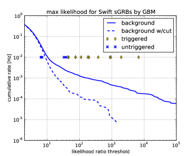
Figure 4: The maximum likelihood coherent flux excess found by searching time around Swift short-GRBs within the GBM field of view using foreground intervals between 0.256 and 2s. GRBs are placed at 0.01 Hz in anticipation of a GW-GBM coincidence search window of $<$100s. An estimated cumulative background rate distribution is found by taking the non-overlapping all-sky events from a continuous scan of approximately one-day in total of nearby data. The dotted background distribution shows the effect of a simple cut to remove particle events (the cut does not remove any GRBs). Of the four un-triggered events, GBM excesses corresponding to GRB 090815C and 110112A are buried within the background distribution, and are not clearly associable with their GRBs. The ability of the method to identify the next two weak, un-triggered events GRBs 090305A and 120403A (see also figure 5) depends on ongoing strategies to further reject non-Gaussian outliers. The remaining Swift sGRB’s in the sample have a corresponding GBM on-board trigger.

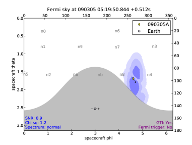
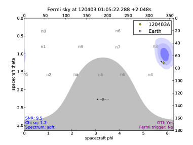
Figure 5: Swift short GRBs (T90 $<$ 2s) 090305A and 120403A were seen by Swift-BAT but did not trigger GBM on-board. Low photon statistics for these weak events result in large sky location uncertainties shown by the 1, 2, and 3$\sigma$ confidence regions. The quoted signal-to-noise ratio is calculated at the best-fit location using the full spectral data from all NaI and BGO detectors. The spectrum represents one of three representative spectral models (hard, normal, soft) for the model response that gives maximum likelihood, while the skymap is marginalized over all spectral models. Arrows represent movement of the Fermi spacecraft over $\pm$2 minutes.

VI Conclusion

Direct detection of gravitational-waves from the merger of NS-NS or NS-BH binary systems is expected to occur within the next few years as advanced 2nd generation ground-based gravitational-wave detectors come online. Fermi GBM provides a unique and promising opportunity to observe EM counterparts due to its large sky coverage, and the anticipated association between NS-NS mergers and sGRB’s. To maximize the use of information from both GWs and GBM, we have outlined a joint search strategy triggered by observations of GW signals from coalescing binary systems in which a small amount of local GBM data is scanned using a likelihood-ratio based analysis applied to the full instrument data. The sensitivity of the method to short GRBs will benefit in the future from continuous GBM offline data products with higher time resolution and improved all-sky response models. We anticipate such an effort will allow sensitive follow-up of NS-NS and NS-BH mergers, most of which are expected to not be accompanied by triggered GRB observation.

VII Acknowledgments

We thank Colleen Wilson-Hodge for assistance with the GBM direct response model. LB is supported by an appointment to the NASA Postdoctoral Program at GSFC, administered by Oak Ridge Associated Universities through a contract with NASA. The authors would also like to acknowledge the support of the NSF through grant PHY-1204371. Finally we thank the Albert Einstein Institute in Hannover, supported by the Max-Planck-Gesellschaft, for use of the Atlas high-performance computing cluster.

References

- Harry (2010) G. M. Harry (LIGO Scientific Collaboration), Class.Quant.Grav. 27, 084006 (2010).
- Accadia et al. (2012) T. Accadia, F. Acernese, F. Antonucci, P. Astone, G. Ballardin, et al., The Twelfth Marcel Grossmann Meeting (Word Scientific, 2012), chap. 313, pp. 1738–1742.
- Willke et al. (2006) B. Willke, P. Ajith, B. Allen, P. Aufmuth, C. Aulbert, et al., Class.Quant.Grav. 23, S207 (2006).
- Somiya (2012) K. Somiya (KAGRA Collaboration), Class.Quant.Grav. 29, 124007 (2012), eprint 1111.7185.
- Schutz (2011) B. F. Schutz, Class.Quant.Grav. 28, 125023 (2011), eprint 1102.5421.
- Weisberg et al. (2010) J. Weisberg, D. Nice, and J. Taylor, Astrophys.J. 722, 1030 (2010), eprint 1011.0718.
- Abadie et al. (2010a) J. Abadie et al. (LIGO Scientific Collaboration, Virgo Collaboration), Class.Quant.Grav. 27, 173001 (2010a), eprint 1003.2480.
- Kouveliotou et al. (1993) C. Kouveliotou, C. A. Meegan, G. J. Fishman, N. P. Bhat, M. S. Briggs, T. M. Koshut, W. S. Paciesas, and G. N. Pendleton, Astrophys.J. 413, L101 (1993).
- Hjorth and Bloom (2011) J. Hjorth and J. S. Bloom (2011), eprint 1104.2274.
- Nakar (2007) E. Nakar, Phys.Rept. 442, 166 (2007), eprint astro-ph/0701748.
- Gehrels et al. (2009) N. Gehrels, E. Ramirez-Ruiz, and D. B. Fox, Ann.Rev.Astron.Astrophys. 47, 567 (2009), eprint 0909.1531.
- Liang et al. (2008) E.-W. Liang, J. L. Racusin, B. Zhang, B.-B. Zhang, and D. N. Burrows, Astrophys.J. 675, 528 (2008), eprint 0708.2942.
- Fong et al. (2012) W.-f. Fong, E. Berger, R. Margutti, B. A. Zauderer, E. Troja, I. Czekala, R. Chornock, N. Gehrels, T. Sakamoto, D. B. Fox, et al. (2012), eprint 1204.5475.
- Grupe et al. (2006) D. Grupe, D. N. Burrows, S. K. Patel, C. Kouveliotou, B. Zhang, P. Mészáros, R. A. M. Wijers, and N. Gehrels, Astrophys.J. 653, 462 (2006), eprint astro-ph/0603773.
- Metzger and Berger (2012) B. Metzger and E. Berger, Astrophys.J. 746, 48 (2012), eprint 1108.6056.
- Coward et al. (2012) D. Coward, E. Howell, T. Piran, G. Stratta, M. Branchesi, O. Bromberg, B. Gendre, R. Burman, and D. Guetta (2012), eprint 1202.2179.
- Troja et al. (2010) E. Troja, S. Rosswog, and N. Gehrels, Astrophys.J. 723, 1711 (2010), eprint 1009.1385.
- Tsang et al. (2012) D. Tsang, J. S. Read, T. Hinderer, A. L. Piro, and R. Bondarescu, Phys.Rev.Lett. 108, 011102 (2012), eprint 1110.0467.
- Meegan et al. (2009) C. Meegan, G. Lichti, P. N. Bhat, E. Bissaldi, M. S. Briggs, V. Connaughton, R. Diehl, G. Fishman, J. Greiner, A. S. Hoover, et al., Astrophys.J. 702, 791 (2009), eprint 0908.0450.
- Abbott et al. (2010) B. Abbott et al. (Virgo Collaboration), Astrophys.J. 715, 1438 (2010), eprint 0908.3824.
- Abadie et al. (2010b) J. Abadie et al. (LIGO Scientific Collaboration, Virgo Collaboration), Astrophys.J. 715, 1453 (2010b), eprint 1001.0165.
- Abadie et al. (2012a) J. Abadie et al. (LIGO Scientific Collaboration), Astrophys.J. 760, 12 (2012a), eprint 1205.2216.
- Abadie et al. (2012b) J. Abadie et al. (LIGO Collaboration, Virgo Collaboration), Phys.Rev. D85, 082002 (2012b), eprint 1111.7314.
- Abadie et al. (2012c) J. Abadie et al. (Virgo Collaboration, LIGO Scientific Collaboration) (2012c), eprint 1203.2674.
- Veitch et al. (2012) J. Veitch, I. Mandel, B. Aylott, B. Farr, V. Raymond, et al., Phys.Rev. D85, 104045 (2012), eprint 1201.1195.
- Fairhurst (2011) S. Fairhurst, Class.Quant.Grav. 28, 105021 (2011), eprint 1010.6192.
- Finger et al. (2009) M. H. Finger, E. Beklen, P. N. Bhat, W. S. Paciesas, V. Connaughton, et al. (2009), eprint 0912.3847.
- Wilson-Hodge et al. (2012) C. A. Wilson-Hodge, G. L. Case, M. L. Cherry, J. Rodi, A. Camero-Arranz, et al., Astrophys.J.Suppl. 201, 33 (2012), eprint 1201.3585.
- Fitzpatrick et al. (2012) G. Fitzpatrick, S. McBreen, V. Connaughton, and M. Briggs (GBM Team) (2012), eprint 1210.5369.
- Paciesas et al. (2012) W. S. Paciesas, C. A. Meegan, A. von Kienlin, P. Bhat, E. Bissaldi, et al., Astrophys.J.Suppl. 199, 18 (2012), eprint 1201.3099.