Abstract

We study form factors in ${\cal N}$=4 SYM at strong coupling in general kinematics and with multi-operator insertions by using gauge/string duality and integrability techniques. This generalizes the $AdS_{3}$ results of Maldacena and Zhiboedov in two non-trivial aspects. The first generalization to $AdS_{5}$ space was motivated by its potential connection to strong coupling Higgs-to-three-gluons amplitudes in QCD which was observed recently at weak coupling. The second generalization to multi-operator insertions was motivated as a step towards applying on-shell techniques to compute correlation functions at strong coupling. In this picture, each operator is associated to a monodromy condition on the cusp solutions. We construct Y-systems for both cases. The $Y$-functions are related to the spacetime (cross) ratios. Their WKB approximations based on a rational function $P(z)$ are also studied. We focus on the short operators, while the prescription is hopefully also applicable for more general operators.

 

 

1 Introduction

One of the most challenging problems of modern theoretical physics is to understand the dynamics of strong coupling QCD analytically. While this is still very difficult, lots of studies have been focused on simpler models such as theories with supersymmetry. The general philosophy is that a good knowledge of these theories may finally help us to understand the real QCD. A particularly interesting theory that has drawn much attention is the ${\cal N}$=4 super Yang-Mills theory. There has been some evidence that ${\cal N}$=4 SYM results are important building blocks of QCD quantities, see for example [1, 2]. By the gauge/string duality, it becomes also possible to study the ${\cal N}$=4 SYM in the strong coupling regime where it is dual to a perturbative or semi-classical string theory in an $AdS$ background [3, 4, 5].

An impressive achievement is that we can now compute anomalous dimensions in ${\cal N}=4$ SYM to any reasonable order in practice, see for example [6, 7, 8, 9, 10], where the integrability of the theory plays a fundamental role [11, 12, 13] (for a review on many aspects of integrability see [14]). It is expected that similar achievement may also be made for other more complicated observables, such as scattering amplitudes and correlation functions. Indeed surprising dualities and integrable structures have been found for amplitudes and null Wilson loops [15, 16, 17, 18, 19, 20, 21], and also correlation functions in a special light-like limit [22, 23].

One remarkable development is the computation of scattering amplitudes in ${\cal N}=4$ SYM at strong coupling [15]. It was shown that the problem can be dual to a string minimal surface problem in $AdS$. The solving of this non-trivial geometrical problem was developed based on the integrability of the classical worldsheet theory [24, 25, 26] . Hopefully, these classical results will be useful to solve the full quantum problem such as in the study of operator dimensions [32, 33].

In this paper, we will focus on a more general class of observables, the so-called form factors. They are observables involving both on-shell particles and off-shell operators, therefore are in some sense hybrids of amplitudes and correlation functions

$$\langle\textrm{Out-states}\,|\,\prod_{i}{\cal O}_{i}(x_{i})\,|\,\textrm{In-states}\rangle\,.$$

We will consider form factors in pure momentum space

$$F(q_{1},\cdots,q_{l};p_{1},\cdots,p_{n})\ =\ \prod_{k=1}^{l}\,\int d^{4}x_{l}\,e^{iq_{k}\cdot x_{k}}\langle{\cal O}(x_{1})\cdots{\cal O}(x_{l})\,|\,p_{1}\cdots p_{n}\rangle\,,$$ (1.1)

where $p_{i}^{2}=0$ and $q_{k}$ is arbitrary.

Most studies so far have been focused on form factors with one operator inserted. Form factors in string theory in $AdS$ were first studied in [34]. Based on the recent developments of strong coupling amplitudes, a T-dual picture of form factors was proposed in [35], and the problem was solved in the $AdS_{3}$ case by using integrability techniques in [36]. At weak coupling, form factors in ${\cal N}=4$ SYM were first studied in [37], and have received attention recently, see for example [38, 39, 40, 41, 42]. One surprising observation in [43] is that the remainder function of a two-loop three-point form factor in ${\cal N}=4$ SYM matches exactly with the maximally transcendental part of the two-loop Higgs-to-3-gluon amplitudes in QCD [44] .

As this correspondence looks very intriguing, one may think that this is an accidental coincidence. However, this two-loop coincidence is already rather non-trivial, which may be appreciated by a simple look at the very different perturbative structures of Feynman diagrams in ${\cal N}=4$ SYM and QCD. It may be therefore reasonable to expect that there could be some hidden relations which will explain this coincidence and might play further roles for other situations, at least for the three-point case due to its particularly simple kinematics . If the two-loop coincidence is going to be true for higher loops, one may expect that strong coupling form factors in ${\cal N}=4$ would carry a non-trivial piece of information of strong coupling QCD. Considering that there are very few tools to study strong coupling QCD amplitudes, this possibility provides us enough motivation to study strong coupling form factors seriously.

The computation of form factors at strong coupling in [36] was restricted to two dimensional kinematics. In such case non-trivial quantities start at four-point. In order to study the three-point form factor, one needs to consider more general kinematics. In this paper we will consider the form factors in full $R^{1,3}$ kinematics, corresponding to string in $AdS_{5}$. As is usually happened, the generalization from $AdS_{3}$ to $AdS_{5}$ is a nontrivial step. Although the underlying picture is similar to the $AdS_{3}$ case, the monodromy structure in $AdS_{5}$ is more complicated. In particular, the truncation conditions involve small solution contractions which are not $T$-functions. This complexity also makes it much more difficult to construct the Y-system, which is a main new challenge of the $AdS_{5}$ problem. We will describe the general construction, and the Y-system for the three-point form factor will be explicitly given.

Another interesting generalization in this paper is to compute form factors with multi-operator insertions. The main motivation is to study correlation functions at strong coupling with the help of on-shell techniques. Similar idea has been used at weak coupling in [46]. Although the observables we consider contain on-shell structures, they involve multiple operators, and in principle should contain all kinds of information of correlation functions. In particular, one should be able to extract the OPE coefficients from form factors containing two or more operators.

The basic idea we propose may be illustrated by the following flow chart 

$\begin{matrix}\begin{tabular}[]{| c |}\hline\cr$\begin{matrix}\,\\ \,\end{matrix}$ Cusps\cr\hline\cr\end{tabular}&\Rightarrow&\begin{tabular}[]{|c|}\hline\cr$\begin{matrix}\,\\ \,\end{matrix}$ Small solutions\cr\hline\cr\end{tabular}&\hskip-14.22636pt\Rightarrow&\begin{tabular}[]{|c|}\hline\cr$\begin{matrix}\,\\ \,\end{matrix}$ Hirota system\cr\hline\cr\end{tabular}\Rightarrow\begin{tabular}[]{|c|}\hline\cr$\begin{matrix}\,\\ \,\end{matrix}$ Y-system\cr\hline\cr\end{tabular}\\ &&\Uparrow&&\\ \begin{tabular}[]{| c |}\hline\cr$\begin{matrix}\,\\ \,\end{matrix}$ Operators\cr\hline\cr\end{tabular}&\Rightarrow&\begin{tabular}[]{|c|}\hline\cr$\begin{matrix}\,\\ \,\end{matrix}$ Monodromy matrices\cr\hline\cr\end{tabular}\,&&\end{matrix}$

The main picture is that for each operator one can define a corresponding monodromy matrix, which will give a linear relation for the small solutions. These small solutions are related to the cusps and are the same building blocks for calculating amplitudes, therefore the known method of computing amplitudes can be applied to these more general class of observables. It is in this sense that we can compute off-shell observables by using on-shell techniques.

We derive explicitly the Y-system for form factors with multi-operator insertions in $AdS_{3}$, while in principle it should be possible to generalize to the $AdS_{5}$ case. The construction proposed in this paper is expected to be in principle applicable to arbitrary operators, although the study will be focused on light operators , for which the monodromy can be given explicitly.

This paper is organized as follows. In Section 2, we review the main physical pictures and the general strategy of strong coupling computation via AdS/CFT and integrability. We then review form factors in the $AdS_{3}$ case in section 3. Form factors in general $AdS_{5}$ kinematics are developed in section 4, and the three-point case is discussed explicitly in section 5. The generalization to multi-operator insertions is given in section 6. In section 7, the $P(z)$ function and WKB approximation are studied. Section 8 contains a summary and some discussions. There are three appendices. Appendix A is a collection of the definition of $T$- and $Y$-functions and their corresponding equations. A review of (momentum) twistor variables is given in appendix B. Appendix C is a brief discussion of the monodromy in a different basis.

2 Classical string and integrable system

Due to the nature of the problem which involves quite a few different stories and intermediate steps, in this section we give a brief review of the whole picture. The discussion here is not supposed to be self-contained, but we hope to cover the key physical pictures and central ideas. Interested reader is referred to the original papers (in particular [24, 25]) for more details.

2.1 Form factor as a classical string solution

As a first step to set up the problem, we explain how to map the computation of amplitudes and form factors at strong coupling in ${\cal N}=4$ SYM to a classical string problem in an $AdS$ background [15, 35].

We first consider the picture for gluon states. Recall the $AdS$ space in Poincaré coordinate

$$ds^{2}\ =\ {dy^{\mu}dy_{\mu}+dz^{2}\over z^{2}}\,.$$ (2.1)

Gluon states in ${\cal N}=4$ SYM are dual to open strings on the IR D3 branes (as an IR regulator) at the horizon (i.e. $z\rightarrow\infty$) [15]. One important property of the open strings on IR branes is that they carry very large proper momenta. Because high energy scattering is dominated by a saddle point approximation [47], the computation of open string amplitude becomes a classical string problem.

Form factors also contain operators, which are dual to closed string states in the bulk with boundary condition at $z\rightarrow 0$ [4, 5]. Therefore form factors correspond to scattering open and closed strings which are from the horizon and the boundary respectively, as shown on the left-hand side of Figure 1 .

To simplify the problem, one important trick is to apply a formal T-duality along $y^{\mu}$ directions [48, 15] . The T-dual space is still an $AdS$ space

$$ds_{\textrm{T-dual}}^{2}\ =\ {dx^{\mu}dx_{\mu}+dr^{2}\over r^{2}}\,,$$ (2.2)

where $r={1/z}$. The boundary and horizon reverse their roles in the T-dual space. The momenta of strings become the “windings” of strings. For amplitudes the problem becomes a type of Wilson loop problem [52, 53], with a null polygonal boundary. For form factors, the boundary becomes a periodic null Wilson line [35], where the period is determined by the momentum of the closed string $q$. The minimal surface extends to the horizon, as illustrated on the right-hand side of Figure 1 .

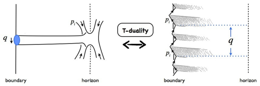
Figure 1: The picture of T-duality for form factor. $q$ is the momentum of the operator which corresponds to a closed string state in the bulk. $q=\sum_{i}p_{i}$ due to momentum conservation. After T-duality, the picture becomes a minimal surface ending on a periodic null Wilson line at the boundary and extending to horizon. The period is given by $q$.

Therefore, the form factor problem becomes to find the area of the minimal surface over one period, with boundary conditions at both the boundary and the horizon of the T-dual $AdS$ space. The general structure of the strong coupling results is

$${\rm Observable}\ =\ e^{-{\sqrt{\lambda}\over 2\pi}\,{\rm Area}}\times({\rm string}\ \alpha^{\prime}\ {\rm corrections})\,,\qquad\alpha^{\prime}\sim{1\over\sqrt{\lambda}}\,.$$ (2.3)

The string corrections in principle may be computed by considering string fluctuations where the classical solution is taking as a background, along the line of [55, 56] .

2.2 String in $AdS$ as a classical integrable system

Because of the non-trivial boundary conditions, it is very hard to solve the string equations. The idea, proposed in [24] (see also for example [60, 61, 62]), is that rather than solving the string equations directly, one can apply the Pohlmeyer’s reduction [63] to reformulate the string equations to a Hitchin like system and then use the techniques of integrability. Here we briefly review the main strategy.

Since Pohlmeyer reduction is a well-understood procedure, we only point out that after the reduction, the string equations of motion and Virasoro constraints take a form of flat equation

$$\partial{\cal A}_{\bar{z}}-\bar{\partial}{\cal A}_{z}+[{\cal A}_{z},{\cal A}_{\bar{z}}]\ =\ 0\,.$$ (2.4)

If one decomposes ${\cal A}$ into two parts ${\cal A}=A+\Phi$, the equations form a Hitchin like system

$$D_{z}\Phi_{\bar{z}}\,=\,0\,,\qquad D_{\bar{z}}\Phi_{z}\,=\,0\,,\qquad[D_{z},D_{\bar{z}}]+[\Phi_{z},\Phi_{\bar{z}}]\,=\,0\,,$$ (2.5)

where $D_{z}:=\partial_{z}+[A_{z},\ ]$. For $AdS_{5}$ case it is a $SU(4)$ system , while for $AdS_{3}$ it can be reduced to $SL(2)$. The flat connection is not arbitrary but satisfies a $Z_{4}$ automorphism

$$A\,=\,-C\,A^{T}\,C^{-1}\,,\qquad\Phi_{z}\,=\,-iC\,\Phi_{z}^{T}\,C^{-1}\,,\qquad\Phi_{\bar{z}}\,=\,iC\,\Phi_{\bar{z}}^{T}\,C^{-1}\,,$$ (2.6)

where $C$ is a constant matrix whose explicit form is not important here. This $Z_{4}$ constraint plays an important role in the construction as we will see later. One can solve the linear equation

$$(d+{\cal A})\,\psi\,=\,0\,,$$ (2.7)

where the solution $\psi$ is related to the target space coordinates and therefore to the string solutions.

A natural logic would be to first find the solution for ${\cal A}$ which solves the Hitchin equations, then solve the linear problem to find the solution $\psi$ which gives the classical string solution. However, the strategy used here is different. Roughly speaking, we will use the properties of the linear solution and the flat connection to construct the area directly without knowing the explicit solution.

The key idea is to use integrability. The integrability can be understood by the fact that one can lift the flat connection to a family of connections

$${\cal A}\ \ \rightarrow\ \ {\cal A}(\zeta)\ =\ \left(A_{z}+{1\over\zeta}\Phi_{z}\right)dz+\left(A_{\bar{z}}+\zeta\Phi_{\bar{z}}\right)d\bar{z}\,,$$ (2.8)

while the Hitchin equations are still satisfied. The new parameter $\zeta$ is called spectral parameter. We also use another variable $\theta$ where $\zeta=e^{i\theta}$. If one solves the linear problem with ${\cal A}(\zeta)$, one obtains a one-parameter family of solutions $\psi(\zeta)$, and the original physical solution can be obtained by taking $\zeta=1$.

With this extra parameter it seems one is dealing with a more general problem. However, new powerful techniques are available based on this new parameter . The main result is that a set of functional equations, so-called Y-system, can be constructed. The non-trivial part of the area can be extracted from the solution of Y-system, which turns out to be the free energy in a thermodynamic Bethe ansatz (TBA) form [66, 67]. For amplitudes in $AdS_{5}$ it is like [26]

$$A_{\rm free}\ =\ \sum_{s}{m_{s}\over 2\pi}\int d\theta\cosh\theta\log\left[(1+Y_{1,s})(1+Y_{3,s})(1+Y_{2,s})^{\sqrt{2}}\right]\,.$$ (2.9)

In this form, area is a function of mass parameters which are implicitly related to the physical cross ratios. An important observation later in [68] is that the area can also be written as the critical value of Yang-Yang functional, and in the new form area can be expressed directly as a function of cross ratios.

2.3 Boundary conditions and function $P(z)$

In this section we explain an important aspect of the story: how to formulate the boundary conditions. This will involve an important holomorphic function $P(z)$. We also discuss the special feature of form factors in which an operator is inserted.

One particular equation of the Hitchin system is the generalized sinh-Gorden equation [25]

$$\partial\bar{\partial}\alpha-e^{\alpha}-e^{-\alpha}|P(z)|\,=\,0\,,$$ (2.10)

where $P$ and $\alpha$ are given as

$$P\,=\,\partial^{2}X\cdot\partial^{2}X\,,\qquad\alpha\,=\,\log(\partial X\cdot\bar{\partial}X)\,.$$ (2.11)

$P(z)$ is a holomorphic function. By making a field redefinition and introducing a new coordinate $w$ by a worldsheet conformal transformation as

$$\alpha(z,\bar{z})\ =\ \hat{\alpha}(z,\bar{z})+{1\over 4}\log P(z)\bar{P}(\bar{z})\,,\qquad dw\ =\ (P(z))^{1/4}dz\ ,$$ (2.12)

one can simplify the generalized sinh-Gordon equation as

$$\partial_{w}\,\bar{\partial}_{\bar{w}}\,\hat{\alpha}-(e^{\hat{\alpha}}+e^{-\hat{\alpha}})\,=\,0\,,$$ (2.13)

which is a simple sinh-Gordon equation. One should note that the change of worldsheet coordinate is only well-defined locally.

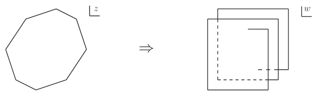
Figure 2: $z$-plane and $w$-plane.

An important fact is that the four-cusp solution (first found in [15]) is simply the solution $P=1$ and $\alpha=\hat{\alpha}=0$ of the generalized sinh-Gordon equation [62]. This is an important reason of doing the above transformation . Asymptotically, the solution near each cusp should be the same as the four-cusp solution. This implies that near boundary where $z\rightarrow\infty$, we should have $\hat{\alpha}\rightarrow 0$. It also implies that each cover of $w$-plane contains four cusps. Therefore, $P(z)$ should be a polynomial, and the degree of the polynomial would depend on the number of cusps. The corresponding picture is shown in Figure 2. The coefficients in the polynomial would encode the shape of the polygon.

A new feature of form factors is that there are also operators. As observed in [36], an insertion of an operator will introduce a pole term in $P(z)$. This requires a study of the boundary condition near the horizon, which will be discussed and generalized to $AdS_{5}$ in section 7. Due to the insertion of operator, the $z$-plane is no longer smooth. One can however smooth the $z$-plane with the sacrifice of introducing a multi-branch-cover of $z$-plane, as illustrated in Figure 3 . This picture is consistent with the periodic null Wilson line picture in the target space. We will use this picture later to introduce the monodromy for small solutions.

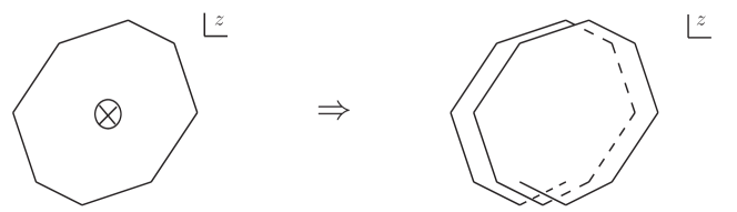
Figure 3: The picture for form factor. An insertion of a operator introduces a singularity in the $z$-plane, and corresponds to a multi-cover of $z$-plane.

2.4 Small solutions

Now we introduce a very important building block, the so-called small solution. Consider again the linear problem

$$\big{(}d+{\cal A}(\zeta,z)\big{)}\,\psi(\zeta,z)\,=\,0\,.$$ (2.14)

Because of the special null-cusp boundary conditions, the solution has different asymptotic behaviors near different cusps. This displays the so-called Stocks phenomenon. The asymptotic behavior of the solution when $z\rightarrow\infty$ is only valid within a given Stokes sector. Let us consider the simple $AdS_{3}$ case (similar picture applies for $AdS_{5}$). While approaching an edge $i$, the solution can be approximated as

$$\psi\ \sim\ c_{i}^{\rm big}\,S_{i}+c_{i}^{\rm small}\,s_{i}\,.$$ (2.15)

Small solutions $s_{i}$ are the solutions which decay fastest while approaching the boundary. They are unique up to a normalization. At first sight, it may be confusing why it is the small solution rather than the big solution that is important. However, it is not the big solution, but the coefficient of the big solution that contains the boundary information. This coefficient can be extracted by contracting the full solution with the small solution as $c_{i}^{\rm big}\sim\langle\psi,s_{i}\rangle$. In this way, all non-trivial boundary information can be obtained in terms of the contraction of small solutions.

The coefficient $c_{i}^{\rm big}$ is related to target-space variable, the momentum twistor $\lambda_{i}$ in the general $AdS_{5}$ case. $\lambda_{i}^{a}$ carries spacetime indices $a$. On the other hand, the small solution $s_{i}^{\alpha}$ is a solution of worldsheet theory and carry internal-space indices $\alpha$. This change of variables from target space coordinates to worldsheet solutions plays a very important role in the strong coupling story.

We now consider the relation between small solutions and the spectral parameter. One important fact is that: the change of the phase of spectral parameter corresponds to the rotation of small solutions (i.e. cusps) . The $Z_{4}$ automorphism mentioned before plays a very important role. For example, the $Z_{2}$ automorphism in $AdS_{3}$ gives the relation $s_{i+1}(\zeta)\propto i\sigma_{3}\,s_{i}(e^{i\pi}\zeta)$. The contraction of small solutions can be defined as T-function and Y-functions, see Appendix A. Using $Z_{4}$ property and some other identities, it is possible to construct a finite set of difference equations between these functions.

While a Y-system is basically a set of algebraic equations given by a set of determinant identities, one needs to provide further information such as the asymptotic behavior of the corresponding functions, so that the obtained solution is corresponding to the observables being studied. This important information can be obtained by WKB approximation, in the limits of the spectral parameter: $|\zeta|\rightarrow 0$ or $\infty$. In such limits, the contraction of small solutions is dominated by an integral along WKB lines that connect different edges, for example in $AdS_{3}$ :

$$\langle s_{i},s_{j}\rangle|_{\zeta\rightarrow 0}\ \sim\ \exp\Big{(}{\int_{i}^{j}{\sqrt{p}\,dz\over\zeta}}\Big{)}\ \sim\begin{tabular}[]{c}{\includegraphics[height=36.98866pt]{smallWKB}}\end{tabular}.$$ (2.16)

The integrand ${\sqrt{p}\,dz/\zeta}$ is obtained as the dominant term of flat connection (2.8) in the limit $\zeta\rightarrow 0$. The WKB lines can be obtained as the parametric curves $z(t)$ which solve the equation ${\rm Im}({\dot{z}\,\sqrt{p}/\zeta})=0$. Therefore they are determined by the function $P(z)$ which is related to the boundary conditions. These will be discussed further in section 7.

One can see that the problem is set up as a Riemann-Hilbert problem (see for example [69]): finding the exact functions from their discontinuities (provided by Y-system equations) and asymptotic behaviors (WKB approximations). In this paper we will construct the Y-systems for form factors in $AdS_{5}$ and with multi-operator insertions in $AdS_{3}$. We also study the WKB approximations.

2.5 Conventions

The basic definitions of $T$- and $Y$-functions and how to obtain Hirota and Y-system equations are summarized in Appendix A. For the reader who is not familiar with the definitions it may be necessary to have a look at the appendix before reading the following sections. Below we mention a few important relations and conventions.

We will often assume the normalization conditions [26]

$$AdS_{3}\ {\rm case}: \quad\langle s_{i},s_{i+1}\rangle\ =\ 1\,,$$ (2.17)

$$AdS_{5}\ {\rm case}: \quad\langle s_{i},s_{i+1},s_{i+2},s_{i+3}\rangle\ =\ 1\,,$$ (2.18)

unless indicated otherwise. The $Z_{4}$ automorphism imposes the following relations [26]

$$AdS_{3}\ {\rm case}: \ s_{i+1}(\zeta)\ =\ i\sigma_{3}\,s_{i}(e^{i\pi}\zeta)\,,$$ (2.19)

$$AdS_{5}\ {\rm case}: \ \bar{s}_{i+1}(\zeta)\ =\ C^{-1}s_{i}(e^{i\pi/2}\zeta)\,,\qquad s_{i+1}(\zeta)\ =\ C^{T}\bar{s}_{i}(e^{i\pi/2}\zeta)\,,$$ (2.20)

where

$$\bar{s}_{i}\ :=\ s_{i-1}\wedge s_{i}\wedge s_{i+1}\,.$$ (2.21)

$\sigma_{3}$ and $C$ are some constant matrices whose explicit forms are not important in this paper.

There are two different conventions used for $AdS_{3}$ and $AdS_{5}$ cases:

$$AdS_{3}\ {\rm case}: \ f^{\pm}:=f(e^{\pm i{\pi\over 2}}\zeta),\qquad f^{[k]}:=f(e^{i{k\pi\over 2}}\zeta)\,,$$ (2.22)

$$AdS_{5}\ {\rm case}: \ f^{\pm}:=f(e^{\pm i{\pi\over 4}}\zeta)\,,\qquad f^{[k]}:=f(e^{i{k\pi\over 4}}\zeta)\,.$$ (2.23)

Since the number of cusps is always even in the $AdS_{3}$ case, for convenience we define

$${\hat{n}}\ :=\ n/2\,,$$ (2.24)

where $n$ is the number of cusps.

3 Review of form factors in $AdS_{3}$

In this section we review the Y-system for form factors in $AdS_{3}$ [36]. The construction in this case is relatively simple, but the basic picture in later generalizations is similar.

3.1 A look at amplitudes

We first look at the case of scattering amplitudes. For amplitudes, the corresponding minimal surface is smooth. The small solutions are single-valued on the $z$ plane

$$s_{j}(e^{i2\pi}z,\zeta)\ =\ s_{j}(z,\zeta)\ .$$ (3.1)

By definition $s_{j+\hat{n}}$ is the small solution in the same sector as $s_{j}$ but after going around the complex $z$ plane once. Because they are the solutions in the same sector, they should be proportional to each other

$$s_{j+{\hat{n}}}(e^{i2\pi}z,\zeta)\ \propto\ s_{j}(z,\zeta)\,.$$ (3.2)

This may be also understood from the periodic condition. Note that an arbitrary proportionality constant is allowed.

To do the contraction of small solutions, one needs to bring two small solutions to the same worldsheet point. Using (3.1) and (3.2), one gets that

$$s_{i+{\hat{n}}}(z,\zeta)\ \propto\ s_{i}(z,\zeta)\,,$$ (3.3)

which implies $\langle s_{i},s_{i+{\hat{n}}}\rangle=0$, or equivalently $T_{\hat{n}-1}=0$. This provides a natural truncation for Hirota equations. The corresponding Y-system is given in terms of $\hat{n}-3$ $Y$-function: $Y_{m}$, $m=1,\ldots,\hat{n}-3$ [26].

3.2 Operator as a monodromy

Now we consider form factors. Since there is an operator inserted, the worldsheet is not smooth but contains a singular point. The small solutions are therefore no longer single-valued on $z$ plane. In other words, they change their values after going around the complex $z$ plane, or more exactly, going around the singular point where the operator is inserted, as shown in Figure 4.

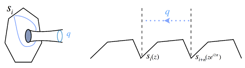
Figure 4: Small solution and monodromy.

This effect can be characterized by introducing a monodromy matrix. One can firstly choose two linearly independent small solutions as a basis. To be explicit, one can choose $\{s_{0},s_{1}\}$. The monodromy is defined as a $2$ by $2$ matrix $\Omega(\zeta)$ satisfying

$$\begin{pmatrix}s_{1}\\ s_{0}\end{pmatrix}(ze^{2\pi i},\zeta)\,=\,\Omega(\zeta)\begin{pmatrix}s_{1}\\ s_{0}\end{pmatrix}(z,\zeta)\ .$$ (3.4)

Using the $Z_{2}$ automorphism relation (2.19), this also fixes the monodromy relations for other small solutions. By taking the wedge of the small solutions, one can obtain

$$\det[\Omega(\zeta)]\,=\,1\,.$$ (3.5)

The exact property of $\Omega$ is determined by the corresponding operator, which can be taken as an input of the system.

By definition, as discussed for amplitudes above, $s_{j+\hat{n}}$ is the small solution in the same sector as $s_{j}$ but after going around the $z$-plane once (see Figure 4). Since they are in the same sector, their relation of proportionality does not change: $s_{j+\hat{n}}(e^{i2\pi}z)\propto s_{j}(z)$. We introduce a proportionality constant $B(\zeta)$ so that

$$s_{\hat{n}}(z,\zeta)=B(\zeta)\,s_{0}(ze^{-2\pi i},\zeta)\,.$$ (3.6)

By $Z_{2}$ relation (2.19), this also determines the proportionality constants for other small solutions, in particular

$$s_{\hat{n}+1}(z,\zeta)\,=\,B^{[2]}(\zeta)s_{1}(ze^{-2\pi i},\zeta)\,.$$ (3.7)

Taking the wedge of small solutions and using the normalization condition one can get a constraint on $B$:

$$B^{-1}\,=\,B^{[2]}\,.$$ (3.8)

At the same point of worldsheet, one obtains

$$\begin{pmatrix}s_{\hat{n}+1}\\ s_{\hat{n}}\end{pmatrix}(z,\zeta)\ =\ {\cal B}(\zeta)\cdot\Omega^{-1}(\zeta)\begin{pmatrix}s_{1}\\ s_{0}\end{pmatrix}(z,\zeta)\,,$$ (3.9)

where the proportionality constants are written into a diagonal matrix

$${\cal B}(\zeta)\,=\,\begin{pmatrix}B^{[2]}(\zeta)&0\\ 0&B(\zeta)\end{pmatrix},\qquad\det[{\cal B}(\zeta)]\,=\,1\,.$$ (3.10)

Unlike amplitudes, $s_{i}$ and $s_{i+\hat{n}}$ are not proportional to each other and $\langle s_{i},s_{i+{\hat{n}}}\rangle\neq 0$, so the truncation becomes much more non-trivial for form factors.

3.3 Truncation and Y-system for form factors

We consider now how to use the above monodromy relation to truncate the Hirota equations, and then how to write them into a Y-system, following [36].

Firstly, a useful relation is from the trace of $\Omega$. From (3.9) one can obtain

$${\rm Tr}[\Omega(\zeta)]\ =\ B(\zeta)\langle s_{0},s_{\hat{n}+1}\rangle(\zeta)-B^{-1}(\zeta)\langle s_{1},s_{\hat{n}}\rangle(\zeta)\,,$$ (3.11)

where we have used the fact that for a $2\times 2$ unitary matrix (${\rm det}[\Omega]=1$), ${\rm Tr}[\Omega]={\rm Tr}[\Omega^{-1}]$. This can be further written as

$${\rm Tr}[\tilde{\Omega}(\zeta)]\ :=\ {\rm Tr}[\Omega(\tilde{\zeta})]=B(\tilde{\zeta})\,T_{\hat{n}}(\zeta)-B^{-1}(\tilde{\zeta})\,T_{\hat{n}-2}(\zeta)\,,$$ (3.12)

where $\tilde{\zeta}=e^{-i({\hat{n}}+1)\pi/2}$.

One can see that the trace relation provides a truncation for the Hirota equations, since one can solve for $T_{\hat{n}}$ in terms of $T_{\hat{n}-2}$ and ${\rm Tr}[\Omega]$. As mentioned before, ${\rm Tr}[\Omega]$ can be taken as an input of the system.

While Hirota equations are not gauge invariant, it is necessary to write the system in a conformally invariant way, i.e. in a form of Y-system. This can be done by defining a new $Y$-function as

$${\overline{Y}}(\zeta)\ :=\ B^{-1}(\tilde{\zeta})\,T_{\hat{n}-2}(\zeta)\,.$$ (3.13)

Then using (3.12), $T_{\hat{n}}(\zeta)$ can be solved as

$$T_{\hat{n}}(\zeta)\ =\ B^{-1}(\tilde{\zeta})\left[{\rm Tr}[\tilde{\Omega}](\zeta)+\overline{Y}(\zeta)\right],$$ (3.14)

and furthermore for $Y_{\hat{n}-1}$

$$Y_{\hat{n}-1}\ =\ T_{\hat{n}-2}\,T_{\hat{n}}\ =\ {\rm Tr}[\tilde{\Omega}]\overline{Y}+\overline{Y}^{2}\ .$$ (3.15)

The equation for $\overline{Y}$ is simply $\overline{Y}^{+}\overline{Y}^{-}=1+Y_{{\hat{n}}-2}$.

In this way, one obtains a set of equations in terms of $\hat{n}-1$ Y-functions:

$$Y_{s}^{+}Y_{s}^{-} = (1+Y_{s+1})(1+Y_{s-1})\,,$$ (3.16)

$$Y_{{\hat{n}}-2}^{+}Y_{{\hat{n}}-2}^{-} = (1+Y_{{\hat{n}}-3})(1+{\rm Tr}[\tilde{\Omega}]\overline{Y}+\bar{Y}^{2}),$$ (3.17)

$$\overline{Y}^{+}\overline{Y}^{-} = 1+Y_{{\hat{n}}-2}\,,$$ (3.18)

where $s=1,\ldots,\hat{n}-3$. A lattice structure of T- and Y-functions is shown in Figure 5.

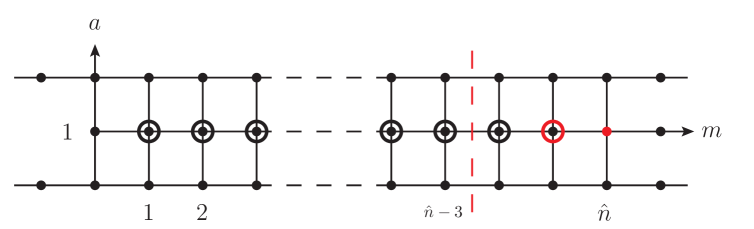
Figure 5: Lattice picture for the Hirota and Y-system of $AdS_{3}$ form factors. Black dots are for functions $T_{a,m}$. Dots with black circles correspond to Y-functions $Y_{a,m}$, while the dot with red circle is for $\overline{Y}$. Red dot is for $T_{\hat{n}}$ which can be solved via the trace relation. For amplitudes, the Y-functions are truncated to the left hand side of the red dashed line.

Comparing to amplitudes, the system contains two new functions $Y_{\hat{n}-2}$ and $\overline{Y}$. This matches with the counting of the degrees of freedom. The operator is associated to the $2\times 2$ monodromy matrix. Because ${\rm det}[\Omega]=1$, there are three independent components, which correspond to three functions: ${\rm Tr}[\Omega]$, $Y_{\hat{n}-2}$ and $\overline{Y}$, while ${\rm Tr}[\Omega]$ is taken as an input in the Y-system . These $\hat{n}-1$ $Y$-functions also match the number of degrees of the T-dual Wilson line picture, which is $2(\hat{n}-1)$.

Because of the simple structure of the above Y-system, it can be easily written in terms of integrable equations. The free energy part of the area can be extracted from the solution and takes a TBA form [36] ,

$$A_{\rm free}\ =\ \sum_{s}{m_{s}\over 2\pi}\int d\theta\cosh\theta\log(1+Y_{s})+2{\overline{m}\over 2\pi}\int d\theta\cosh\theta\log(1+\overline{Y})\,.$$ (3.19)

For the $AdS_{3}$ case here, the construction of Y-system looks straightforward and simple. As we will see later, the generalizations to $AdS_{5}$ and to multi-operator insertions are much more involving. However, the underlying picture is similar.

We would like to emphasize again how the picture of operator enters the story. The basic building blocks are small solutions, which are related to the null-cusp structure. The operator is introduced by a monodromy matrix which imposes some linear relations on the small solutions. The method of computing null Wilson loops can then be applied in a similar way to compute form factors. The detailed information of the monodromy is taken as an input. In principle one may consider arbitrary operators, depending on the choice of corresponding monodromy matrices.

3.4 Spacetime picture

Finally, in this subsection we review the spacetime picture [36]. We first clarify the difference between the worldsheet monodromy and spacetime monodromy. Then we solve the monodromy and also write the $\overline{Y}$-functions in terms of target-space variables which specify the spacetime boundary configuration.

There are two kinds of monodromy. One is defined in terms of small solutions, as discussed above. It characterizes the non-single-valuedness of small solutions while going around the path that surrounds the operator. We call it worldsheet monodromy and denote it as $\Omega$. The other one is defined in terms of spacetime variables. It will be called spacetime monodromy and denoted by $\hat{\Omega}$.

The spacetime monodromy can be taken as a spacetime conformal transformation. It can be given by mapping $\{X_{n},X_{n+1},X_{n+2}\}$ to $\{X_{0},X_{1},X_{2}\}$. Using spinor decomposition $X_{i}=\lambda^{L}_{i}\lambda^{R}_{i}$, it is enough to consider left-hand spinor $\lambda^{L}_{i}$ . Explicitly, the monodromy can be defined as

$$\lambda^{L}_{i+n}\ \propto\ \hat{\Omega}\,\lambda^{L}_{i}\ =\ \begin{pmatrix}\hat{\Omega}_{11}\lambda^{L}_{i,1}+\hat{\Omega}_{12}\lambda^{L}_{i,2}\\ \hat{\Omega}_{21}\lambda^{L}_{i,1}+\hat{\Omega}_{22}\lambda^{L}_{i,2}\end{pmatrix},$$ (3.20)

where $i=0,1,2$. Because $X_{i}$’s are embedding coordinates, the mapping is only projectively, and an arbitrary proportionality constant is allowed for each $i$. One also has $\det(\hat{\Omega})=1$, because the conformal group is $SL(2,R)$.

The trace truncation equation (3.11) in terms of spacetime variables can be written as

$${\rm Tr}[\hat{\Omega}]\langle\lambda^{L}_{0},\lambda^{L}_{1}\rangle\ =\ \langle\lambda^{L}_{0},\hat{\Omega}\lambda^{L}_{1}\rangle+\langle\hat{\Omega}\lambda^{L}_{0},\lambda^{L}_{1}\rangle\,.$$ (3.21)

Unlike the worldsheet picture where monodromy relates different small solutions, in spacetime the monodromy matrix operates on a single spinor variable. The worldsheet monodromy $\Omega_{ij}$ carries the indices of small solution basis, while the spacetime monodromy $\hat{\Omega}_{ab}$ carries spacetime indices. For each component of $\hat{\Omega}_{ij}$ and $\Omega_{ab}$, they are in general different from each other. But for special combinations like ${\rm Tr}[\Omega]$, the worldsheet and spacetime monodromies take the same value [36].

One can solve for $\hat{\Omega}$ more explicitly in terms of Poincaré coordinate $x$. It is convenient to use light-cone coordinates $x^{\pm}:=x_{0}\pm x_{1}$, which can be related to spinors as [24]

$$x^{+}_{i}\,=\,{(\lambda^{L}_{i})_{2}\over(\lambda^{L}_{i})_{1}}\,.$$ (3.22)

The monodromy relations (3.20) written in terms of $x^{+}$ variables are

$${1\over x_{i+\hat{n}}^{+}}\ =\ {\hat{\Omega}_{11}+\hat{\Omega}_{12}x_{i}^{+}\over\hat{\Omega}_{21}+\hat{\Omega}_{22}x_{i}^{+}}\,,$$ (3.23)

where $i=0,1,2$. Together with the condition $\det(\hat{\Omega})=1$, they uniquely fix the monodromy (up to a whole sign).

We focus on the short operators which is T-dual to a null Wilson line boundary condition. One has

$$x_{i+\hat{n}}^{+}\ =\ x_{i}^{+}+q\,,$$ (3.24)

for all $i$. Using (3.23), one can obtain the monodromy

$$\hat{\Omega}\ =\ \begin{pmatrix}1&0\\ q&1\end{pmatrix},$$ (3.25)

and ${\rm Tr}[\hat{\Omega}]=2$. As shown in [36], the trace of the worldsheet monodromy takes the same value

$${\rm Tr}[\Omega]\ =\ {\rm Tr}[\hat{\Omega}]\ =\ 2\,.$$ (3.26)

The $\overline{Y}$-function can be also written in terms of spacetime variables. To do this one needs first to write the $\overline{Y}$ function in a form which is independent of normalization. One can define $\tilde{s}_{1}(z)=s_{1}(ze^{-i2\pi})$ and therefore $\langle s_{\hat{n}},\tilde{s}_{1}\rangle=B\langle s_{\hat{n}},s_{\hat{n}+1}\rangle$. Recall the definition (3.13), one obtains

$$\overline{Y}(\zeta)\ =\ {\langle s_{1},s_{\hat{n}}\rangle\over\langle s_{\hat{n}},\tilde{s}_{1}\rangle}(\zeta e^{-i\pi(n+1)/2})\,.$$ (3.27)

This form makes it obvious that the WKB approximation of $\overline{Y}$ forms a closed path which contains the singular point corresponding to the insertion of operator [36].

Then ${\overline{Y}}$ can be written in terms of spacetime coordinates

$$\overline{Y}(\zeta=i^{\hat{n}+1})\ =\ {\langle\lambda^{L}_{1},\lambda^{L}_{\hat{n}}\rangle\over\langle\lambda^{L}_{\hat{n}},\hat{\Omega}\lambda^{L}_{1}\rangle}=-{\lambda^{L}_{1,1}\lambda^{L}_{\hat{n},2}-\lambda^{L}_{1,2}\lambda^{L}_{\hat{n},1}\over\lambda^{L}_{1,1}\lambda^{L}_{\hat{n},2}-(q\lambda^{L}_{1,1}+\lambda^{L}_{1,2})\lambda^{L}_{\hat{n},1}}={x_{1,\hat{n}}^{+}\over x_{\hat{n},\hat{n}+1}^{+}}\ .\$$ (3.28)

One can see that $\overline{Y}$ is scale-invariant, but different from other $Y$-functions which are usual conformal cross ratios. This is related to the fact that form factor is not dual-conformally invariant, unlike scattering amplitudes. The nice point is that at strong coupling in the worldsheet picture, integrability techniques are still available. One can deal with $\overline{Y}$ exactly in the same way as for usual $Y$-functions.

4 Form factors in $AdS_{5}$

In this section, we study form factors in $AdS_{5}$. The construction will be parallel to the $AdS_{3}$ case, but as we will see, new problems will appear.

4.1 Monodromy

As in $AdS_{3}$, one can first choose four linearly independent small solutions $\{s_{-2},s_{-1},s_{0},s_{1}\}$ as a basis for the general solutions of the linear problem. The worldsheet monodromy is characterized by a 4 by 4 matrix $\Omega(\zeta)$, which is defined by the relation

$$\begin{pmatrix}s_{1}\\ s_{0}\\ s_{-1}\\ s_{-2}\end{pmatrix}(ze^{2\pi i},\zeta)\ =\ \Omega^{-1}(\zeta)\begin{pmatrix}s_{1}\\ s_{0}\\ s_{-1}\\ s_{-2}\end{pmatrix}(z,\zeta)\,.$$ (4.1)

Taking the wedge of small solutions one has $\det[\Omega(\zeta)]=1$.

By definition, one has the same proportionality relation that $s_{j+n}(e^{i2\pi}z,\zeta)\propto s_{j}(z,\zeta)$. We introduce the proportionality constant $B(\zeta)$ such that

$$s_{n+1}(z,\zeta)\ =\ B(\zeta)\,s_{1}(e^{-2\pi i}z,\zeta)\,.$$ (4.2)

Using the $Z_{4}$ automorphism relations (2.20), proportionality constants are fixed for all other small solutions, in particular

$$s_{n}(z,\zeta) = B^{-1}(e^{i\pi/2}\zeta)\,s_{0}(e^{-2\pi i}z,\zeta)\,,$$ (4.3)

$$s_{n-1}(z,\zeta) = B(e^{-i\pi}\zeta)\,s_{-1}(e^{-2\pi i}z,\zeta)\,,$$ (4.4)

$$s_{n-2}(z,\zeta) = B^{-1}(e^{-i\pi/2}\zeta)\,s_{-2}(e^{-2\pi i}z,\zeta)\,.$$ (4.5)

There are also extra constraints from (2.20):

$$B\,B^{[4]}\,=\,B^{[2]}B^{[-2]}\,,\qquad B\,=\,B^{[8]}\,.$$ (4.6)

One obtains that at the same point of the worldsheet $s_{j}$ and $s_{j+n}$ are related to each other as

$$\begin{pmatrix}s_{n+1}\\ s_{n}\\ s_{n-1}\\ s_{n-2}\end{pmatrix}(z,\zeta)\ =\ {\cal B}^{-1}(\zeta)\cdot\Omega(\zeta)\begin{pmatrix}s_{1}\\ s_{0}\\ s_{-1}\\ s_{-2}\end{pmatrix}(z,\zeta)\,,$$ (4.7)

where the proportionality factors are written into a diagonal matrix

$${\cal B}^{-1}\ :=\ {\rm diag}\big{\{}B,(B^{[2]})^{-1},B^{[-4]},(B^{[-2]})^{-1}\big{\}}\,,\qquad\det[{\cal B}]=1\,.$$ (4.8)

4.2 Truncation of Hirota equations

Similar to the $AdS_{3}$ case, one can apply trace conditions to truncate the Hirota equations. The traces of monodromy are conformally invariant quantities [36]. Their spacetime picture will be discussed later. We first consider the simple trace ${\rm Tr}[\Omega]=\sum_{i=1}^{4}\Omega_{ii}$. Using (4.7), one can obtain

$${\rm Tr}[\Omega] = {\cal B}_{11}\,\langle s_{-2},s_{-1},s_{0},s_{n+1}\rangle+{\cal B}_{44}\,\langle s_{n-2},s_{-1},s_{0},s_{1}\rangle$$ (4.9)

$$+\,{\cal B}_{33}\,\langle s_{-2},s_{n-1},s_{0},s_{1}\rangle+{\cal B}_{22}\,\langle s_{-2},s_{-1},s_{n},s_{1}\rangle\,.$$

Using the definition of $T$-functions, this can be further written as

$${\rm Tr}[\Omega]\ =\ {\cal B}_{11}\ T^{[n]}_{1,n}-{\cal B}_{44}\ T^{[n-1]}_{3,n-3}-{\cal B}_{22}\,\langle s_{-2},s_{-1},s_{1},s_{n}\rangle+\,{\cal B}_{33}\,\langle s_{-2},s_{0},s_{1},s_{n-1}\rangle\,,$$ (4.10)

which provides a truncation for the chain of Hirota equations by expressing $T_{1,n}$ in terms of other $T$ functions. One may worry about the other two terms which are not $T$ functions. However, they can be expressed in terms of $T$-functions as will be discussed in the next subsection.

To obtain a truncation relation for $T_{3,n}$, it is natural to consider the $\bar{s}_{i}$ variables and the corresponding $\overline{\Omega},\overline{\cal B}$, which gives 

$${\rm Tr}[\overline{\Omega}]\ =\ {\overline{\cal B}}_{11}\ T^{[n]}_{3,n}-{\overline{\cal B}}_{44}\ T^{[n-1]}_{1,n-3}-{\overline{\cal B}}_{22}\,\langle\bar{s}_{-2},\bar{s}_{-1},\bar{s}_{1},\bar{s}_{n}\rangle+\,{\overline{\cal B}}_{33}\,\langle\bar{s}_{-2},\bar{s}_{0},\bar{s}_{1},\bar{s}_{n-1}\rangle\,.$$ (4.11)

Note that $\bar{\Omega},\bar{\cal B}$ are not new but related to $\Omega,{\cal B}$, see Appendix C.

Finally, we need a truncation relation for $T_{2,n}$. One can consider the double trace (see also [70])

$${\rm Tr}^{(2)}[\Omega]\ :=\ \sum_{1\leq i<j\leq 4}\Omega_{ii}\,\Omega_{jj}={1\over 2}\left({\rm Tr}[\Omega]^{2}-{\rm Tr}[\Omega^{2}]\right)\,.$$ (4.12)

Using (4.7) and the definition of $T$ functions, one obtains

$${\rm Tr}^{(2)}[\Omega] = {\cal B}_{11}\,{\cal B}_{22}\ T_{2,n}^{[n-1]}+{\cal B}_{33}\,{\cal B}_{44}\ T_{2,n-4}^{[n-1]}$$ (4.13)

$$-{\cal B}_{11}\,{\cal B}_{33}\,\langle s_{-2},s_{0},s_{n-1},s_{n+1}\rangle-{\cal B}_{22}\,{\cal B}_{44}\,\langle s_{-1},s_{1},s_{n-2},s_{n}\rangle$$

$$+{\cal B}_{11}\,{\cal B}_{44}\,\langle s_{-1},s_{0},s_{n-2},s_{n+1}\rangle+{\cal B}_{22}\,{\cal B}_{33}\,\langle s_{-2},s_{1},s_{n-1},s_{n}\rangle\,.$$

As will be discussed in next subsection, all small solution contractions can be written in terms of $T$ functions. One may consider further a relation from the triple-trace

$${\rm Tr}^{(3)}[\Omega]:=\sum_{i<j<k}\Omega_{ii}\,\Omega_{jj}\,\Omega_{kk}={1\over 6}\left({\rm Tr}[\Omega]^{3}-3\,{\rm Tr}[\Omega^{2}]\,{\rm Tr}[\Omega]+2\,{\rm Tr}[\Omega^{3}]\right)\,,$$ (4.14)

but it can be shown that it gives an equivalent truncation relation for $T_{1,n}$ function.

4.3 Recursion relations

In the above truncation relations, several new small solution contractions appear. In this subsection we show that they can be expressed in terms of $T$-functions by using some recursion relations. A few new functions will be defined for convenience.

We define the contractions appearing in simple-trace relations as $R$- and $S$-functions

$$R_{1,m}\ :=\ \langle s_{-2},s_{-1},s_{1},s_{m+2}\rangle^{[-m]}\,,\qquad R_{3,m}\ :=\ \langle\bar{s}_{-2},\bar{s}_{-1},\bar{s}_{1},\bar{s}_{m+2}\rangle^{[-m]}\,,\qquad$$ (4.15)

$$S_{1,m}\ :=\ \langle s_{-2},s_{0},s_{1},s_{m+2}\rangle^{[-m]}\,,\qquad\ \ S_{3,m}\ :=\ \langle\bar{s}_{-2},\bar{s}_{0},\bar{s}_{1},\bar{s}_{m+2}\rangle^{[-m]}\,.$$ (4.16)

Using the Wronskian relations reviewed in Appendix A, one can obtain the following recursion relations

$$R_{1,m}\ =\ R^{-}_{1,m-1}{T^{+}_{1,m+1}\over T_{1,m}}+{T_{2,m+1}\over T_{1,m}}\,,\qquad R_{3,m}\ =\ R^{-}_{3,m-1}{T^{+}_{3,m+1}\over T_{3,m}}+{T_{2,m+1}\over T_{3,m}}\,,\qquad$$ (4.17)

$$S_{1,m}\ =\ S_{1,m-1}^{-}{T_{3,m}^{[2]}\over T_{3,m-1}^{+}}-{T_{2,m-1}^{[2]}\over T_{3,m-1}^{+}}\,,\qquad\ S_{3,m}\ =\ S_{3,m-1}^{-}{T_{1,m}^{[2]}\over T_{1,m-1}^{+}}-{T_{2,m-1}^{[2]}\over T_{1,m-1}^{+}}\,.$$ (4.18)

Together with the initial conditions

$$R_{1,0}=R_{3,0}=T_{2,1}\,,\qquad S_{1,0}=T_{1,1},S_{3,0}=T_{3,1}\,,$$ (4.19)

all $R$- and $S$-functions can be expressed in terms of $T$-functions.

To consider the contractions appearing in the double-trace relation, we first define

$$U_{1,m}\ :=\ \langle s_{-2},s_{-1},s_{m},s_{m+2}\rangle^{[-m]}\,, U_{3,m}\ :=\ \langle s_{-1},s_{0},s_{m+1},s_{m+3}\rangle^{[-m-2]}\,,$$ (4.20)

$$V_{1,m}\ :=\ \langle s_{-2},s_{0},s_{m+1},s_{m+2}\rangle^{[-m]}\,, V_{3,m}\ :=\ \langle s_{-1},s_{1},s_{m+2},s_{m+3}\rangle^{[-m-2]}\,,$$ (4.21)

which satisfy

$$U_{1,m}={T^{-}_{1,m-1}T_{2,m+1}+T^{+}_{1,m+1}T^{-}_{2,m}\over T_{1,m}}\,, U_{3,m}={T^{-}_{3,m-1}T_{2,m+1}+T^{+}_{3,m+1}T^{-}_{2,m}\over T_{3,m}}\,,$$ (4.22)

$$V_{1,m}={T^{+}_{1,m-1}T_{2,m+1}+T^{-}_{1,m+1}T^{+}_{2,m}\over T_{3,m}}\,, V_{3,m}={T^{+}_{3,m-1}T_{2,m+1}+T^{-}_{3,m+1}T^{+}_{2,m}\over T_{1,m}}\,.$$ (4.23)

The four contractions in (4.13) are then defined as

$$W_{1,m}(\zeta):=\langle s_{-2},s_{0},s_{m+1},s_{m+3}\rangle^{[-m-1]}, W_{3,m}(\zeta):=\langle s_{-1},s_{1},s_{m+2},s_{m+4}\rangle^{[-m-3]},$$ (4.24)

$$W_{2,m}(\zeta):=\langle s_{-1},s_{0},s_{m+1},s_{m+4}\rangle^{[-m-2]}, {\overline{W}}_{2,m}(\zeta):=\langle s_{-2},s_{1},s_{m+2},s_{m+3}\rangle^{[-m-2]},\ \ \ \ \$$ (4.25)

which satisfy

$$W_{1,m}={V^{-}_{1,m}U^{+}_{3,m}-T^{-}_{1,m}T^{+}_{1,m}\over T_{2,m}}\,,\qquad\qquad W_{3,m}={V^{-}_{3,m}U^{+}_{1,m}-T^{-}_{3,m}T^{+}_{3,m}\over T_{2,m}}\,,$$ (4.26)

$$W_{2,m}={U^{+}_{3,m+1}U_{3,m}-T^{-}_{2,m}T^{+}_{2,m+2}\over T_{2,m+1}}\,,\qquad{\overline{W}}_{2,m}={V^{-}_{1,m+1}V_{3,m}-T^{+}_{2,m}T^{-}_{2,m+2}\over T_{2,m+1}}\,.\qquad$$ (4.27)

Using (4.22)-(4.23), all $W$-functions can be written in terms of $T$-functions.

The main lesson in this subsection is that any small solution contraction can be expressed in terms of $T$-functions, therefore it is enough to focus on the $T$-functions.

4.4 Y-system for $AdS_{5}$ form factors

While it is straightforward to introduce the trace relations to truncate the Hirota system, it is more challenging to obtain a Y-system.

We find it mostly convenient to introduce three new ${\overline{Y}}_{a}$ functions as follows:

$${\overline{Y}}_{1}\ :=\ A_{1}\,{T_{3,n-2}\over T_{2,n-1}}\,,\qquad{\overline{Y}}_{3}\ :=\ A_{3}\,{T_{1,n-2}\over T_{2,n-1}}\,,\qquad{\overline{Y}}_{2}\ :=\ A_{2}\,{T_{2,n-2}\over T_{1,n-1}T_{3,n-1}}\,,$$ (4.28)

where

$$A_{1}\ :=\ B^{[-n]}\,,\qquad A_{3}\ :=\ (B^{[-n+4]})^{-1}\,,\qquad A_{2}\ :=\ {B^{[-n+1]}\over B^{[-n+3]}}\,.$$ (4.29)

It is interesting to notice the relations

$${A_{2}^{+}A_{2}^{-}\over A_{1}A_{3}}\ =\ {A_{1}^{+}A_{3}^{-}\over A_{2}}\ =\ {A_{1}^{-}A_{3}^{+}\over A_{2}}\ =\ 1\,,$$ (4.30)

which have appeared for the amplitudes of $n=4K$ cases for three special combinations of Y-functions (see page 27 of [26]).

These ${\overline{Y}}$ functions satisfy the following nice equations

$${{\overline{Y}}_{1}^{+}{\overline{Y}}_{3}^{-}\over{\overline{Y}}_{2}}\ =\ {1+Y_{3,n-2}\over 1+Y_{2,n-1}}\,,\qquad\quad{{\overline{Y}}_{1}^{-}{\overline{Y}}_{3}^{+}\over{\overline{Y}}_{2}}\ =\ {1+Y_{1,n-2}\over 1+Y_{2,n-1}}\,,$$ (4.31)

$${{\overline{Y}}_{2}^{+}{\overline{Y}}_{2}^{-}\over{\overline{Y}}_{1}{\overline{Y}}_{3}}\ =\ {1+Y_{2,n-2}\over(1+Y_{1,n-1})(1+Y_{3,n-1})}\,.$$ (4.32)

Notice that functions $Y_{a,n-1}$ appear on the right-hand side of equations. To have a closed system, one needs to solve them in terms of other $Y$-functions. This can be done by noticing the following relations 

$$Y_{a,n-1}\ =\ (A_{a}^{-1}\,T_{a,n}){\overline{Y}}_{a}\,,\qquad a=1,2,3\,,$$ (4.33)

while $A_{a}^{-1}\,T_{a,n}$ can be solved directly using the trace relations given before. Since the trace functions of $\Omega$ are normalization independent, the trace equations (and therefore $Y_{a,n-1}$) are guaranteed to be able to be written in terms of $Y$-functions: ${\overline{Y}}_{a}$ and $Y_{a,m},m=1,\ldots,n-2$. This will be shown explicitly later in the three-point case.

The full Y-system for form factors in $AdS_{5}$ can be summarized as

$${Y^{-}_{a,m}Y^{+}_{4-a,m}\over Y_{a+1,m}Y_{a-1,m}}\ =\ {(1+Y_{a,m+1})(1+Y_{4-a,m-1})\over(1+Y_{a+1,m})(1+Y_{a-1,m})}\,,$$ (4.34)

$${{\overline{Y}}_{a}^{+}{\overline{Y}}_{4-a}^{-}\over{\overline{Y}}_{a+1}{\overline{Y}}_{a-1}}\ =\ {1+Y_{a,n-2}\over(1+Y_{a+1,n-1})(1+Y_{a-1,n-1})}\,,$$ (4.35)

where $a=1,2,3,\ \ m=1,\ldots,n-2$, and $Y_{a,n-1}$ can be expressed in terms of other $Y$-functions appearing in the equations. Therefore one obtains a closed finite system in terms of $3(n-1)$ $Y$-functions, as shown in Figure 6.

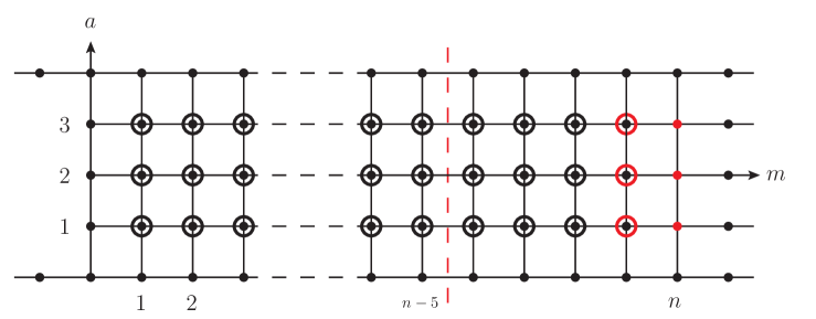
Figure 6: Lattice picture for the T/Y-system of $AdS_{5}$ form factors. Dots with black circles correspond to Y-functions $Y_{a,m}$, while dots with red circles are for $\overline{Y}$. Red dots are for $T_{a,n}$ which can be solved via the trace relations. For amplitudes, the Y-functions are truncated to the left hand side of the red dashed line.

Comparing to amplitudes where there are $3(n-5)$ $Y$-functions, in form factors there are $12$ more (for $n>4$). This can be understood as follows. Form factor contains a $4\times 4$ unitary monodromy matrix $\Omega$ which has 15 independent components. Minus three traces, 12 degrees of freedom are left, giving 12 new $Y$-functions. On the other hand, this does not match with the spacetime picture of a periodic Wilson line in $AdS_{5}$, where it only has $3n-7$ independent degrees of freedom . Note this is different from the $AdS_{3}$ case, where the number of $Y$-functions matches with the number of the degrees of freedom. It implies that in $AdS_{5}$, the monodromy matrix of a short operator is not arbitrary but with extra four constraints. In practice this is not a problem, since the WKB approximation of $Y$-functions are determined in the same way by the $P(z)$ polynomial. For general operators, it would require further information.

A proposal for the free energy

Following the result in $AdS_{3}$ [36], a natural proposal for the free energy is

$$A_{\rm free} = \sum_{s}{m_{s}\over 2\pi}\int d\theta\cosh\theta\log\left[(1+Y_{1,s})(1+Y_{3,s})(1+Y_{2,s})^{\sqrt{2}}\right]$$ (4.36)

$$+c\,{\overline{m}\over 2\pi}\int d\theta\cosh\theta\log\left[(1+{\overline{Y}}_{1})(1+{\overline{Y}}_{3})(1+{\overline{Y}}_{2})^{\sqrt{2}}\right],$$

where $c$ is an integer factor which may be fixed by studying some simple limits.

4.5 Reduction to $AdS_{4}$ and $AdS_{3}$

We consider the reduction following the discussion for amplitudes in [26]. The reduction to the $AdS_{4}$ case is simply given by taking

$$T_{1,s}(\zeta)\ =\ T_{3,s}(\zeta)\,,\qquad Y_{1,s}(\zeta)\ =\ Y_{3,s}(\zeta)\,.$$ (4.37)

Therefore for form factors in $AdS_{4}$, there are only two trace-relations ${\rm Tr}[\Omega]$ and ${\rm Tr}^{(2)}[\Omega]$ to consider. This reduction will be used in the three-point case.

We consider further to reduce the system to $AdS_{3}$. Besides the relation $T_{1,s}=T_{3,s}$, the linear problem splits into two decoupled problems denoted by $left$ and $right$ problems. In an appropriate gauge

$$s_{2k}\ =\ \begin{pmatrix}s^{R}_{k}\\ 0\end{pmatrix},\qquad s_{2k+1}\ =\ \begin{pmatrix}0\\ s^{L}_{k+1}\end{pmatrix}\,,$$ (4.38)

where $s^{L}$ and $s^{R}$ are the small solution of the left and right $AdS_{3}$ problems respectively. The left and the right problems are related by a rotation in the spectral parameter

$$\langle s^{R}_{i},s^{R}_{j}\rangle\ =\ \langle s^{L}_{i},s^{L}_{j}\rangle^{[2]}\,.$$ (4.39)

The small solution contraction in $AdS_{5}$ is reduced to

$$\langle s_{2i},s_{2k+1},s_{2j},s_{2l+1}\rangle\ =\ -\,\langle s^{R}_{i},s^{R}_{j}\rangle\,\langle s^{L}_{k+1},s^{L}_{l+1}\rangle\,.$$ (4.40)

One can choose a normalization $\langle s^{L}_{i},s^{L}_{i+1}\rangle=1$, this corresponds to an unusual normalization $\langle s_{i},s_{i+1},s_{i+2},s_{i+3}\rangle=-1$ in $AdS_{5}$. Most equations in $AdS_{5}$ become identically satisfied except for the nodes of $T_{2,2k}$. For these, they reduce to the Hirota equations in $AdS_{3}$.

The monodromy matrix can be decomposed as

$$\begin{pmatrix}s_{1}\\ s_{-1}\\ s_{0}\\ s_{-2}\end{pmatrix}(ze^{2\pi i},\zeta)\ \sim\ \begin{pmatrix}\Omega_{L}(\zeta)&0\\ 0&\Omega_{R}(\zeta)\end{pmatrix}\begin{pmatrix}s_{1}\\ s_{-1}\\ s_{0}\\ s_{-2}\end{pmatrix}(z,\zeta)\,,$$ (4.41)

where using the relation $s_{R,a}=s_{L,a}^{[2]}$, one can get

$$\Omega_{R}\ =\ \Omega_{L}^{[-2]}\,.$$ (4.42)

One can check that the three traces-relations in $AdS_{5}$ exactly reduce to the single relation in $AdS_{3}$. In deriving it one needs to use the relation

$$\rm Tr[\Omega]\ =\ -(\rm Tr[\Omega_{L}]+\rm Tr[\Omega_{R}])\,,$$ (4.43)

while the minus sign is due to the normalization $\langle s_{i},s_{i+1},s_{i+2},s_{i+3}\rangle=-1$.

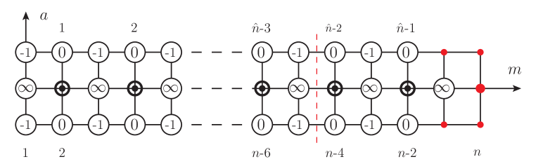
Figure 7: The reduction of $AdS_{5}$ $Y$-functions to $AdS_{3}$. Most $Y$-functions become trivial (i.e. -1, 0 or $\infty$ as shown in the figure), while half of $Y_{2,m}$-functions are reduced to $AdS_{3}$ $Y$-functions. Interestingly, the three $\overline{Y}_{a}$-functions do not reduce to $\overline{Y}$-functions in $AdS_{3}$. Red dots are related only to $T_{\hat{n}}$-functions in $AdS_{3}$.

The reduction of $Y$ functions can be summarized as in Figure 7.

4.6 Spacetime picture

As discussed in the $AdS_{3}$ case, the spacetime monodromy can be understood as a spacetime conformal transformation. In $AdS_{5}$ it is convenient to consider the map for twistor variables, and in this representation the conformal group is $SU(4)$. An introduction of twistor variables is given in Appendix B.

Spacetime monodromy can be defined by mapping four twistors $\{\lambda_{n-2},\lambda_{n-1},\lambda_{n},\lambda_{n+1}\}$ to $\{\lambda_{-2},\lambda_{-1},\lambda_{0},\lambda_{1}\}$

$$\lambda_{i+n}\ \propto\ \hat{\Omega}\,\lambda_{i}\,,$$ (4.44)

where $i=-2,-1,0,1$. Note that the map is only projective, and an arbitrary proportionality constant is allowed for each $i$. Since $\hat{\Omega}\in SU(4)$, one has $\det(\hat{\Omega})=1$. Like for small solutions, we also define

$$\bar{\lambda}_{i}^{a}\ :=\ \epsilon^{abcd}\,\lambda_{b}\,\lambda_{c}\,\lambda_{d}\,,$$ (4.45)

and the corresponding monodromy $\hat{\bar{\Omega}}$ is defined as $\bar{\lambda}_{i+n}\propto\hat{\bar{\Omega}}\,\bar{\lambda}_{i}$, where $i=-2,-1,0,1$.

The single trace relation written in terms of spacetime variables corresponds to

$${\rm Tr}[\hat{\Omega}]\,\langle\lambda_{-2},\lambda_{-1},\lambda_{0},\lambda_{1}\rangle\ =\ \langle\hat{\Omega}\lambda_{-2},\lambda_{-1},\lambda_{0},\lambda_{1}\rangle+\langle\lambda_{-2},\hat{\Omega}\lambda_{-1},\lambda_{0},\lambda_{1}\rangle$$ (4.46)

$$\hskip 128.0374pt+\langle\lambda_{-2},\lambda_{-1},\hat{\Omega}\lambda_{0},\lambda_{1}\rangle+\langle\lambda_{-2},\lambda_{-1},\lambda_{0},\hat{\Omega}\lambda_{1}\rangle\,,$$

and similar from ${\rm Tr}[\hat{\bar{\Omega}}]$. For double trace one has

$${\rm Tr}^{(2)}[\hat{\Omega}]\,\langle\lambda_{-2},\lambda_{-1},\lambda_{0},\lambda_{1}\rangle\ =\ \langle\hat{\Omega}\lambda_{-2},\hat{\Omega}\lambda_{-1},\lambda_{0},\lambda_{1}\rangle+\langle\lambda_{-2},\lambda_{-1},\hat{\Omega}\lambda_{0},\hat{\Omega}\lambda_{1}\rangle\qquad$$ (4.47)

$$\hskip 128.0374pt+\langle\hat{\Omega}\lambda_{-2},\lambda_{-1},\hat{\Omega}\lambda_{0},\lambda_{1}\rangle+\langle\lambda_{-2},\hat{\Omega}\lambda_{-1},\lambda_{0},\hat{\Omega}\lambda_{1}\rangle$$

$$\hskip 128.0374pt+\langle\lambda_{-2},\hat{\Omega}\lambda_{-1},\hat{\Omega}\lambda_{0},\lambda_{1}\rangle+\langle\hat{\Omega}\lambda_{-2},\lambda_{-1},\lambda_{0},\hat{\Omega}\lambda_{1}\rangle\,,$$

where

$${\rm Tr}^{(2)}[\hat{\Omega}]\ :=\ \sum_{1\leq i<j\leq 4}\hat{\Omega}_{ii}\,\hat{\Omega}_{jj}\ =\ {1\over 2}\left({\rm Tr}[\hat{\Omega}]^{2}-{\rm Tr}[\hat{\Omega}^{2}]\right).$$ (4.48)

One can solve for the monodromy in terms of the Lorentz variables. We will focus on short operators which correspond to periodic boundary conditions. The transformation between twistor variables and Lorentz variables is reviewed in Appendix B. The derivation of the monodromy may be given in two different ways.

Firstly one has the relations (B.6)

$$x^{-}_{j}\,=\,i\,{\lambda^{j}_{[1}\,\lambda^{j+1}_{4]}\over\lambda^{j}_{[1}\,\lambda^{j+1}_{2]}}\,,\qquad x^{+}_{j}\,=\,i\,{\lambda^{j}_{[2}\,\lambda^{j+1}_{3]}\over\lambda^{j}_{[1}\,\lambda^{j+1}_{2]}}\,,$$ (4.49)

where $x^{\pm}=x^{1}\pm x^{0}$. Without loss of generality, one can choose the periodic direction to be along $x^{1}$-direction

$$x^{\mu}_{j+n}\ =\ x^{\mu}_{j}+q\,\delta^{1,\mu}\,,\qquad x^{\pm}_{j+n}\ =\ x^{\pm}_{j}+q\,.$$ (4.50)

Using (4.44), one can obtain

$$x_{j+n}^{-} = i\,{\hat{\Omega}_{1a}\,\hat{\Omega}_{4b}\,\lambda^{j}_{[a}\,\lambda^{j+1}_{b]}\over\hat{\Omega}_{1a}\,\hat{\Omega}_{2b}\,\lambda^{j}_{[a}\,\lambda^{j+1}_{b]}}\ =\ i\,{\lambda^{j}_{[1}\,\lambda^{j+1}_{4]}-i\,q\,\lambda^{j}_{[1}\,\lambda^{j+1}_{2]}\over\lambda^{j}_{[1}\,\lambda^{j+1}_{2]}}\ ,$$ (4.51)

$$x_{j+n}^{+} = i\,{\hat{\Omega}_{2a}\,\hat{\Omega}_{3b}\,\lambda^{j}_{[a}\,\lambda^{j+1}_{b]}\over\hat{\Omega}_{1a}\,\hat{\Omega}_{2b}\,\lambda^{j}_{[a}\,\lambda^{j+1}_{b]}}\ =\ i\,{\lambda^{j}_{[2}\,\lambda^{j+1}_{3]}-i\,q\,\lambda^{j}_{[1}\,\lambda^{j+1}_{2]}\over\lambda^{j}_{[1}\,\lambda^{j+1}_{2]}}\,,$$ (4.52)

for all $j$. These relations fix the monodromy uniquely as

$$\hat{\Omega}\ =\ \begin{pmatrix}1&0&0&0\\ 0&1&0&0\\ i\,q&0&1&0\\ 0&-i\,q&0&1\end{pmatrix}.$$ (4.53)

There is another simpler way to find the monodromy. From the definition of twistor variable (B.10), one can obtain

$$\lambda_{j}\ \propto\ (\Lambda_{j}\,,\,\mu_{j})\,,\qquad\lambda_{j+n}\ \propto(\Lambda_{j}\,,\,\mu_{j}-i\,q\cdot\Lambda_{j})\,,$$ (4.54)

or equivalently,

$$\lambda_{j+n}\ =\ b_{j}\,\hat{\Omega}\,\lambda_{j}\,,$$ (4.55)

where $\hat{\Omega}$ is given by the same matrix as above, when $q$ is along $x^{1}$-direction . A proportionality constant $b_{i}$ is introduced explicitly, which plays a similar role as the $B$ factor defined for small solutions. Note the relation $\Lambda_{n+i}=b_{i}\,\Lambda_{i}$.

One obtains that

$${\rm Tr}[\hat{\Omega}]={\rm Tr}[\hat{\bar{\Omega}}]=4\,,\qquad{\rm Tr}^{(2)}[\hat{\Omega}]=6\,.$$ (4.56)

As in [36], one can shown that the corresponding traces of worldsheet monodromy take the same value, which can be taken as an input of the Y-system.

Next we consider to write $\overline{Y}_{a}$ function in terms of spacetime variables. To do this, one needs first to write them in a form independent of normalization. To make the derivation simpler, one may recall the relation ${\overline{Y}}_{a}=Y_{a,n-1}/(A_{a}^{-1}\,T_{a,n})$. Since $Y_{a,n-1}$ is a normal cross ratios, one can focus on $(A_{a}^{-1}\,T_{a,n})$, which is similar to the $AdS_{3}$ case.

Consider first the $\overline{Y}_{1}$ case. One can define $\tilde{s}_{-2}(z)=s_{-2}(ze^{-i2\pi})=B^{[-2]}s_{n-2}(z)$, and therefore $\langle\tilde{s}_{-2},s_{n-1},s_{n},s_{n+1}\rangle=B^{[-2]}\langle s_{n-2},s_{n-1},s_{n},s_{n+1}\rangle$. One has the correspondence

$$(A_{1}^{-1}T_{1,n})(\zeta)\ \rightarrow\ {\langle s_{-2},s_{n-1},s_{n},s_{n+1}\rangle\over\langle\tilde{s}_{-2},s_{n-1},s_{n},s_{n+1}\rangle}(\zeta e^{-i\pi{n-2\over 4}})\,.$$ (4.57)

Together with the expression of $Y_{1,n-1}$, this gives

$${\overline{Y}}_{1}(\zeta)\ =\ {\langle\tilde{s}_{-2},s_{n-1},s_{n},s_{n+1}\rangle\langle s_{-1},s_{n-2},s_{n-1},s_{n}\rangle\over\langle s_{-2},s_{-1},s_{n-1},s_{n}\rangle\langle s_{n-2},s_{n-1},s_{n},s_{n+1}\rangle}(\zeta e^{-i\pi{n-2\over 4}})\,,$$ (4.58)

which looks almost like a cross ratio. It also makes it obvious that the WKB lines of $\overline{Y}$ form a closed contour which contains the singular point corresponding to the insertion of operator.

The normalization-independent form can be written directly in terms of spacetime coordinates as

$${\overline{Y}}_{1}(\zeta=i^{{n-2\over 2}}) = {\langle\hat{\Omega}\lambda_{-2},\lambda_{n-1},\lambda_{n},\lambda_{n+1}\rangle\langle\lambda_{-1},\lambda_{n-2},\lambda_{n-1},\lambda_{n}\rangle\over\langle\lambda_{-2},\lambda_{-1},\lambda_{n-1},\lambda_{n}\rangle\langle\lambda_{n-2},\lambda_{n-1},\lambda_{n},\lambda_{n+1}\rangle}\,.$$ (4.59)

One can obtain the other two $\overline{Y}$-functions in the same way. The normalization independent forms are

$${\overline{Y}}_{3}(\zeta) = {\langle\tilde{s}_{-3},\tilde{s}_{-2},\tilde{s}_{-1},s_{n}\rangle\langle s_{-2},s_{-1},s_{0},s_{n-1}\rangle\over\langle s_{-2},s_{-1},s_{n-1},s_{n}\rangle\langle s_{-3},s_{-2},s_{-1},s_{0}\rangle}(\zeta e^{-i\pi{n-2\over 4}})\,,$$

$$\qquad{\overline{Y}}_{2}(\zeta) = {\langle\tilde{s}_{-2},\tilde{s}_{-1},s_{n},s_{n+1}\rangle\langle s_{-1},s_{0},s_{n-1},s_{n}\rangle\over\langle s_{-2},s_{-1},s_{0},s_{n}\rangle\langle s_{-1},s_{n-1},s_{n},s_{n+1}\rangle}(\zeta e^{-i\pi{n-1\over 4}})\,,$$ (4.60)

and in terms of spacetime coordinates they are

$${\overline{Y}}_{3}(\zeta=e^{i\pi{n-2\over 4}}) = {\langle\hat{\Omega}\lambda_{-3},\hat{\Omega}\lambda_{-2},\hat{\Omega}\lambda_{-1},\lambda_{n}\rangle\langle\lambda_{-2},\lambda_{-1},\lambda_{0},\lambda_{n-1}\rangle\over\langle\lambda_{-2},\lambda_{-1},\lambda_{n-1},\lambda_{n}\rangle\langle\lambda_{-3},\lambda_{-2},\lambda_{-1},\lambda_{0}\rangle}\,,$$

$$\qquad{\overline{Y}}_{2}(\zeta=e^{i\pi{n-1\over 4}}) = {\langle\hat{\Omega}\lambda_{-2},\hat{\Omega}\lambda_{-1},\lambda_{n},\lambda_{n+1}\rangle\langle\lambda_{-1},\lambda_{0},\lambda_{n-1},\lambda_{n}\rangle\over\langle\lambda_{-2},\lambda_{-1},\lambda_{0},\lambda_{n}\rangle\langle\lambda_{-1},\lambda_{n-1},\lambda_{n},\lambda_{n+1}\rangle}\,.$$ (4.61)

Using the results in Appendix B, it is also easy to write them in terms of Lorentz variables.

5 Three-point form factor

In this section we study more explicitly the three-point case. This case is interesting because of its potential connection to QCD quantities as reviewed in the introduction. It also provides an example to show explicitly how to write the truncation relations in terms of only Y-functions.

The three trace equations for the $n=3$ case are given as

$${\rm Tr}[\Omega] = {\cal B}_{11}\,T^{[3]}_{1,3}+\,{\cal B}_{33}\,T^{-}_{1,1}-{\cal B}_{22}\,R_{1,1}^{+}\,,$$ (5.1)

$${\rm Tr}[\overline{\Omega}] = \overline{\cal B}_{11}\,T^{[3]}_{3,3}+\,\overline{\cal B}_{33}\,T^{-}_{3,1}-\overline{\cal B}_{22}\,R_{3,1}^{+}\,,$$ (5.2)

$${\rm Tr}^{(2)}[\Omega] = {\cal B}_{11}\,{\cal B}_{22}\,T_{2,3}^{[2]}+{\cal B}_{22}\,{\cal B}_{33}\,T_{1,2}+{\cal B}_{11}\,{\cal B}_{44}\,T_{3,2}^{[4]}-{\cal B}_{11}\,{\cal B}_{33}\,W_{1,1}^{[2]}\,,\qquad$$ (5.3)

where, using the relations in section 4.3,

$$R_{1,1}\ =\ {T_{2,1}^{-}\,T_{1,2}^{+}+T_{2,2}\over T_{1,1}}\,,\qquad R_{3,1}\ =\ {T_{2,1}^{-}\,T_{3,2}^{+}+T_{2,2}\over T_{3,1}}\,,\qquad$$ (5.4)

$$W_{1,1}\ =\ -\,{T^{-}_{1,1}\,T^{+}_{1,1}\over T_{2,1}}+{(T_{2,2}^{+}+T_{2,1}T_{3,2}^{[2]})(T_{2,2}^{-}+T_{2,1}T_{1,2}^{[-2]})\over T_{2,1}\,T_{3,1}^{+}\,T_{3,1}^{-}}\,.$$ (5.5)

These provide the truncation for the Hirota system by expressing $T_{a,3}$ through $T_{a,1}$, $T_{a,2}$ and the traces.

To construct the Y-system, one can notice that using the definition of Y-functions, the T-functions can be solved in terms of $Y$-functions (with also $A$ factors defined in (4.29)):

$$T_{1,1}={A_{1}\over Y_{2,1}{\overline{Y}}_{1}}\,,\qquad T_{3,1}={A_{3}\over Y_{2,1}{\overline{Y}}_{3}}\,,\qquad T_{2,1}={A_{2}\over Y_{1,1}Y_{3,1}{\overline{Y}}_{2}}\,,$$ (5.6)

$$T_{1,2}={A_{2}\over Y_{3,1}{\overline{Y}}_{2}}\,,\qquad T_{3,2}={A_{2}\over Y_{1,1}{\overline{Y}}_{2}}\,,\qquad T_{2,2}={A_{1}A_{3}\over Y_{2,1}{\overline{Y}}_{1}{\overline{Y}}_{3}}\,.\qquad$$ (5.7)

One can then substitute these expressions for $T$ functions into the trace equations. The only thing which may cause trouble are the $A$ factors. They need to be cancelled since the expressions should be gauge invariant. Indeed, after a little calculation, one can express the trace conditions explicitly in terms of only Y-functions:

$${\rm Tr}[\Omega] = {Y_{1,2}^{[3]}\over{\overline{Y}}_{1}^{[3]}}+{1\over Y_{2,1}^{-}{\overline{Y}}_{1}^{-}}-{1\over{\overline{Y}}_{3}^{+}}\left(1+{{\overline{Y}}_{1}^{+}{\overline{Y}}_{3}^{+}\over{\overline{Y}}_{2}{\overline{Y}}_{2}^{[2]}}{Y_{2,1}^{+}\over Y_{1,1}Y_{3,1}^{[2]}}{1\over Y_{3,1}}\right),$$ (5.8)

$${\rm Tr}[\overline{\Omega}] = {Y_{3,2}^{[3]}\over{\overline{Y}}_{3}^{[3]}}+{1\over Y_{2,1}^{-}{\overline{Y}}_{3}^{-}}-{1\over{\overline{Y}}_{1}^{+}}\left(1+{{\overline{Y}}_{1}^{+}{\overline{Y}}_{3}^{+}\over{\overline{Y}}_{2}{\overline{Y}}_{2}^{[2]}}{Y_{2,1}^{+}\over Y_{3,1}Y_{1,1}^{[2]}}{1\over Y_{1,1}}\right),$$ (5.9)

$${\rm Tr}^{(2)}[\Omega] = {Y_{2,2}^{[2]}\over{\overline{Y}}_{2}^{[2]}}+{1\over Y_{3,1}{\overline{Y}}_{2}}+{1\over Y_{1,1}^{[4]}{\overline{Y}}_{2}^{[4]}}-{{\overline{Y}}_{3}^{+}{\overline{Y}}_{3}^{[3]}\over{\overline{Y}}_{2}{\overline{Y}}_{2}^{[2]}{\overline{Y}}_{2}^{[4]}}{Y_{2,1}^{+}\over Y_{1,1}^{[2]}Y_{3,1}}{Y_{2,1}^{[3]}\over Y_{1,1}^{[4]}Y_{3,1}^{[2]}}$$

$$\hskip 2.84544pt-\,{{\overline{Y}}_{3}^{+}\over{\overline{Y}}_{1}^{[3]}{\overline{Y}}_{2}}{Y_{2,1}^{+}\over Y_{3,1}}-{{\overline{Y}}_{3}^{[3]}\over{\overline{Y}}_{1}^{+}{\overline{Y}}_{2}^{[4]}}{Y_{2,1}^{[3]}\over Y_{1,1}^{[4]}}-{{\overline{Y}}_{2}^{[2]}\over{\overline{Y}}_{1}^{+}{\overline{Y}}_{1}^{[3]}}\left(Y_{1,1}^{[2]}Y_{3,1}^{[2]}-{Y_{1,1}^{[2]}Y_{3,1}^{[2]}\over Y_{2,1}^{+}Y_{2,1}^{[3]}}\right).$$

All $A$ factors are cancelled exactly. This provides a non-trivial consistency check for our construction. As claimed before, $Y_{a,2}$ can be expressed in terms of other Y-functions and the trace functions. The final Y-system is a closed system in terms of six Y-functions: three $Y_{a,1}$ and three $\overline{Y}_{a}$.

5.1 Reduction to $AdS_{4}$

A three-cusp periodic Wilson line can be always embedded in an $AdS_{4}$ subspace of $AdS_{5}$. Therefore, one can simplify the system further to $AdS_{4}$. As mentioned before, in $AdS_{4}$ one has $Y_{1,m}=Y_{3,m}$. The Y-system equations are given as

$${Y^{-}_{1,1}Y^{+}_{1,1}\over Y_{2,1}}\ =\ {1+Y_{1,2}\over 1+Y_{2,1}}\,, {Y^{-}_{2,1}Y^{+}_{2,1}\over Y_{1,1}^{2}}\ =\ {1+Y_{2,2}\over(1+Y_{1,1})^{2}}\,,$$ (5.11)

$${{\overline{Y}}_{1}^{+}{\overline{Y}}_{1}^{-}\over{\overline{Y}}_{2}}\ =\ {1+Y_{1,1}\over 1+Y_{2,2}}\,, {{\overline{Y}}_{2}^{+}{\overline{Y}}_{2}^{-}\over{\overline{Y}}_{1}^{2}}\ =\ {1+Y_{2,1}\over(1+Y_{1,2})^{2}}\,,$$ (5.12)

where by the trace condition and also using (4.56),

$$Y_{1,2} = {\overline{Y}}_{1}\left[4-{1\over Y_{2,1}^{[-4]}{\overline{Y}}_{1}^{[-4]}}+{1\over{\overline{Y}}_{1}^{[-2]}}\left(1+{{\overline{Y}}_{1}^{2}\over{\overline{Y}}_{2}^{-}{\overline{Y}}_{2}^{+}}{Y_{2,1}\over Y_{1,1}^{-}Y_{1,1}^{+}}{1\over Y_{1,1}^{-}}\right)^{[-2]}\right],$$ (5.13)

$$Y_{2,2} = {\overline{Y}}_{2}\left[6-{1\over Y_{1,1}^{[-2]}{\overline{Y}}_{2}^{[-2]}}-{1\over Y_{1,1}^{[2]}{\overline{Y}}_{2}^{[2]}}+{{\overline{Y}}_{1}^{-}{\overline{Y}}_{1}^{+}\over{\overline{Y}}_{2}{\overline{Y}}_{2}^{[-2]}{\overline{Y}}_{2}^{[2]}}{Y_{2,1}^{-}\over Y_{1,1}^{[-2]}Y_{1,1}}{Y_{2,1}^{+}\over Y_{1,1}Y_{1,1}^{[2]}}\right.$$

$$\hskip 14.22636pt\left.+{{\overline{Y}}_{1}^{-}\over{\overline{Y}}_{1}^{+}{\overline{Y}}_{2}^{[-2]}}{Y_{2,1}^{-}\over Y_{1,1}^{[-2]}}+{{\overline{Y}}_{1}^{+}\over{\overline{Y}}_{1}^{-}{\overline{Y}}_{2}^{[2]}}{Y_{2,1}^{+}\over Y_{1,1}^{[2]}}+{{\overline{Y}}_{2}\over{\overline{Y}}_{1}^{-}{\overline{Y}}_{1}^{+}}\left(Y_{1,1}^{2}-{Y_{1,1}^{2}\over Y_{2,1}^{-}Y_{2,1}^{+}}\right)\right].$$

This is the Y-system which has potential connection to strong coupling leading transcendental piece  of Higgs-to-3-gluons amplitudes in QCD. Note that one may also use (5.11)-(5.12) to rewrite them into other forms, in particular to change the phase shift of some $Y$ functions.

The WKB approximation of Y-functions is determined only by the $P(z)$ function

$$P(z)\ =\ {a_{-1}\over z}+{1\over z^{2}}\,,$$ (5.15)

which will be discussed in more details in section 7. The degrees of freedom also match: the complex number $a_{-1}$ provides two real parameters, while the three-cusp periodic Wilson line has also two independent ratios variables.

The equations (5.13) and (5.1) looks a little complicated. In particular, a new feature is that some functions have large phase-shift which is beyond the physical strip $(-\pi/4,\pi/4)$. This will make it a little more complicated to write them in the form of integral equations, as the extra pole contributions need to be carefully considered. We leave this problem to another study.

Finally, we consider to express the Y-functions in terms of spacetime coordinates. As in the weak coupling, it is convenient to consider following variables

$$u\ :=\ {p_{12}^{2}\over q^{2}},\qquad v\ :=\ {p_{23}^{2}\over q^{2}},\qquad w\ :=\ {p_{31}^{2}\over q^{2}}\,,$$ (5.16)

where $p_{ij}:=p_{i}+p_{j}$. There are only two independent variables since

$$q^{2}\ =\ p_{12}^{2}+p_{23}^{2}+p_{31}^{2}\,,\qquad u+v+w\,=\,1\,.$$ (5.17)

The $Y$ functions in terms of these variables can be obtained as (see Appendix B)

$$\overline{Y}_{1}(\zeta=e^{i\pi/4})\ =\ {\langle\lambda_{-1},\lambda_{1},\lambda_{2},\lambda_{3}\rangle\over b_{-2}\,\langle\lambda_{-2},\lambda_{-1},\lambda_{2},\lambda_{3}\rangle}={1\over 1/(1-w)+1}\,,$$ (5.18)

$$\overline{Y}_{2}(\zeta=i)\ =\ {\langle\lambda_{1},\lambda_{2},\lambda_{3},\lambda_{4}\rangle\langle\lambda_{-1},\lambda_{0},\lambda_{2},\lambda_{3}\rangle\over b_{-2}\,b_{-1}\,\langle\lambda_{-2},\lambda_{-1},\lambda_{0},\lambda_{3}\rangle\langle\lambda_{-1},\lambda_{2},\lambda_{3},\lambda_{4}\rangle}={v\over u\,w}\,,$$ (5.19)

$$Y_{1,1}(\zeta=i)\ =\ {\langle\lambda_{-2},\lambda_{-1},\lambda_{0},\lambda_{3}\rangle\langle\lambda_{-1},\lambda_{0},\lambda_{1},\lambda_{2}\rangle\over\langle\lambda_{-1},\lambda_{0},\lambda_{2},\lambda_{3}\rangle\langle\lambda_{-2},\lambda_{-1},\lambda_{0},\lambda_{1}\rangle}=-{u\,w\over v}\,,$$ (5.20)

$$Y_{2,1}(\zeta=e^{i\pi/4})\ =\ {\langle\lambda_{-2},\lambda_{-1},\lambda_{2},\lambda_{3}\rangle\langle\lambda_{-1},\lambda_{0},\lambda_{1},\lambda_{2}\rangle\over\langle\lambda_{-1},\lambda_{1},\lambda_{2},\lambda_{3}\rangle\langle\lambda_{-2},\lambda_{-1},\lambda_{0},\lambda_{2}\rangle}={w\over 1-w}\Big{(}{1\over 1-w}+1\Big{)}\,.$$ (5.21)

One can compare them with the interesting set of variables necessarily appearing at weak coupling[43] in constructing functions via the so-called symbol technique [71]:

$$\left\{u,v,w,1-u,1-v,1-w,1-\frac{1}{u},1-\frac{1}{v},1-\frac{1}{w},-\frac{uv}{w},-\frac{vw}{u},-\frac{wu}{v}\right\}.$$ (5.22)

One can see that similar combinations appear in $Y$ functions. This is like the six-gluon amplitude case, where the variables in the symbol construction [71] correspond to the Y-functions at strong coupling . The three-point form factor provides a further evidence that the “correct” variables for constructing functions from symbols at weak coupling, which is hard to know (usually only through guess work), may be read directly from Y-functions.

6 Form factors with multi-operator insertions

In this section we consider form factors with multi-operator insertions

$$F(q_{1},\cdots,q_{l};p_{1},\cdots,p_{n})\ =\ \prod_{k=1}^{l}\,\int d^{4}x_{l}\,e^{iq_{k}\cdot x_{k}}\,\langle{\cal O}(x_{1})\cdots{\cal O}(x_{l})\,|\,p_{1}\cdots p_{n}\rangle\,.$$ (6.1)

We first propose a dual picture for such observables. Then we construct Y-system for the $AdS_{3}$ case, with arbitrary number of operator insertions.

6.1 Evidence at weak coupling

We first recall the picture of form factors with a single operator insertion. After T-duality, the picture involves a periodic null Wilson line boundary condition. The period is defined by the momentum of the operator. A duality between form factors and periodic Wilson lines was also found at weak coupling at one-loop [38]. A dual MHV rule description was proved for tree and one-loop form factors and also proposed to higher loops in [40].

How about a form factor with more than one operators? A natural generalization is that in the T-dual picture, every operator will generate a periodic direction. For operator ${\cal O}_{i}(q_{i})$, the corresponding period is $q_{i}$. Such picture for form factor with two-operator inserted is shown in Figure 8. It is given by a two dimensional periodic lattice and is associated to a Torus topology. For general $m$-operator insertions, the corresponding topology is ${\mathds{T}}^{m}$. The momentum space can be parametrized by introducing new coordinates $x^{(k)}_{i}$, which are defined as

$$x_{i+1}-x_{i}=x^{(k)}_{i+1}-x^{(k)}_{i}=p_{i}\,,\ \qquad\ x^{(k)}_{i+n}-x_{i}=q_{k}\,,$$ (6.2)

$$x_{i+n}-x_{i}=x^{(k)}_{i+n}-x^{(k)}_{i}=Q\,,\ \qquad\ Q:=\sum_{k=1}^{l}q_{k}\,,$$ (6.3)

where $k=1,\ldots,l$, and $l$ is the number of operators. See Figure 8 for the $l=2$ case.

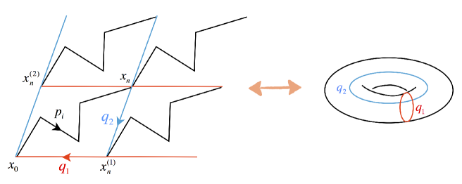
Figure 8: The dual momentum space configuration for form factors with two-operator inserted. There are two periodic directions which give a periodic two dimensional lattice picture. This is equivalent to a torus.

One particular support of this dual picture is that the dual MHV rule description [40] also applies to such generalized configuration, which provides an evidence that this dual picture may apply more generally.

In next subsection we will consider the worldsheet picture, where the introduction of multi-monodormy seems to be a natural generalization of the single insertion case. As we will discuss later in subsection 6.5, the monodromies in terms of the above spacetime coordinates can be also naturally defined.

6.2 Small solution and multi-monodromy

We first introduce the picture of path $\gamma_{k}$ on the worldsheet, as shown in Figure 9. $\gamma_{k}$ is defined as a path that goes around the singular point $z_{k}$ where the operator ${\cal O}_{k}$ is inserted. A special path is $\gamma_{\infty}$ which surrounds all poles. This special path is similar to that of the single-operator case, $ze^{\oint\gamma_{\infty}}\sim ze^{i2\pi}$, in the sense that effectively one can take the combination of all operators as one composite operator.

Next we introduce small solutions $s_{i}$ and $s_{i}^{(k)}$. This is inspired by the spacetime picture of $x_{i}$ and $x_{i}^{(k)}$ considered in last subsection, see Figure 8.

The set of small solutions $s_{i}$ is related to the special path $\gamma_{\infty}$. As mentioned above, they behave similarly as those of the form factor with a single operator inserted, as one can take all operators effectively as a single operator. Therefore one has the same relations

$$s_{\hat{n}}(z,\zeta)\ =\ B(\zeta)\,s_{0}(ze^{-\oint\gamma_{\infty}},\zeta)\,,$$ (6.4)

$$\begin{pmatrix}s_{1}\\ s_{0}\end{pmatrix}(ze^{\oint\gamma_{\infty}},\zeta)\ =\ \Omega(\zeta)\begin{pmatrix}s_{1}\\ s_{0}\end{pmatrix}(z,\zeta)\,,$$ (6.5)

as the form factor studied in section 3. Using this set of small solutions, one can also define the $T$- and $Y$-functions and construct the Y-system equations in exactly the same way. The monodromy $\Omega$ should correspond to the product of the monodromies of all operators.

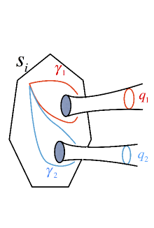
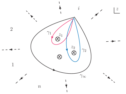
Figure 9: Multi-monodromy picture on the string world-sheet.

The small solutions $s^{(k)}_{i}$ is similar to the dual coordinate $x_{i}^{(k)}$ in spacetime. Because of the periodic structure, each set of small solutions $s^{(k)}_{i}$ with fixed $k$ is not different from the set of small solutions $s_{i}$. One has $\langle s^{(k)}_{i},s^{(k)}_{j}\rangle=\langle s_{i},s_{j}\rangle$. Similarly the $Z_{2}$ automorphism relations also apply such that $s^{(k)}_{i+1}(\zeta)=i\sigma_{3}\,s^{(k)}_{i}(e^{i\pi}\zeta)$.

The information of monodromy is encoded in the relation between $s_{i}$ and $s^{(k)}_{j}$.

Recall that by definition, $s_{\hat{n}+i}$ is the small solution in the same sector as $s_{i}$ but after going around the complex $z$-plane (more exactly the path $\gamma_{\infty}$ which surrounds all operators) once, therefore they should be proportional with each other as given in (6.4). Similarly, $s^{(k)}_{\hat{n}+i}$ is defined as a small solution in the same sector as $s_{i}$ but after going around the path $\gamma_{k}$ once, as shown in Figure 9. One also has the proportionality relation $s^{(k)}_{\hat{n}+i}(z,\zeta)\propto s_{i}(ze^{-\oint\gamma_{k}},\zeta)$. One can introduce proportionality constants $B^{(k)}$ as

$$s^{(k)}_{\hat{n}}(z,\zeta)\ =\ B^{(k)}\,s_{0}(ze^{-\oint\gamma_{k}},\zeta)\,.$$ (6.6)

Because of the insertion of operators, small solutions are not single-valued. For each path $\gamma_{k}$, one can define a corresponding monodromy matrix as

$$\begin{pmatrix}s_{1}\\ s_{0}\end{pmatrix}(ze^{\oint\gamma_{k}},\zeta)\ =\ \Omega^{(k)}(\zeta)\begin{pmatrix}s_{1}\\ s_{0}\end{pmatrix}(z,\zeta)\,,$$ (6.7)

which is similar to the single insertion case.

At the same worldsheet point, one has

$$\begin{pmatrix}s^{(k)}_{\hat{n}+1}\\ s^{(k)}_{\hat{n}}\end{pmatrix}(z,\zeta)\ =\ {\cal B}^{(k)}(\zeta)\cdot(\Omega^{(k)})^{-1}(\zeta)\begin{pmatrix}s_{1}\\ s_{0}\end{pmatrix}(z,\zeta)\,,$$ (6.8)

where

$${\cal B}^{(k)}(\zeta)\ =\ \begin{pmatrix}(B^{(k)})^{[2]}(\zeta)&0\\ 0&B^{(k)}(\zeta)\end{pmatrix},\qquad\det[{\cal B}^{(k)}(\zeta)]=1\,,$$ (6.9)

and similar relation between the $s_{i+\hat{n}}$ and $s_{i}$ as (3.9). Since $e^{\oint\gamma_{\infty}}=\prod_{k=1}^{l}e^{\oint\gamma_{k}}$, one has

$$\Omega\ =\ \prod_{k=1}^{l}\,\Omega^{(k)}\,.$$ (6.10)

Note that the order of operators should be not important, which implies that $\Omega^{(k)}$ should commute with each other. This requirement imposes further constraints on the monodromy matrices as will be discussed later .

6.3 New T and Y functions

Now we consider the definition of $T$ and $Y$ functions and their relations. As we mentioned before, if one just focuses on the set of small solution $s_{i}$, one obtains a Y-system exactly the same as the single operator case, with the total monodromy $\Omega$. The same Y-system can be constructed for the set of small solutions $s^{(k)}_{i}$ with fixed $k$, since $\langle s_{i},s_{j}\rangle=\langle s^{(k)}_{i},s^{(k)}_{j}\rangle$. The new degrees of freedom due to multi-operator insertions are contained in the interplay between small solutions $s_{i}$ and $s^{(k)}_{i}$, which would necessarily involve the monodromy $\Omega^{(k)}$.

We define new $T$-functions as

$$\begin{array}[]{lll}T^{(k)}_{1,2m+1}\ :=\ \langle s_{-m-1},s^{(k)}_{m+1}\rangle,&&T^{(k)}_{1,2m}\ :=\ \langle s_{-m-1},s^{(k)}_{m}\rangle^{+},\\ T^{(k)}_{0,2m}\ :=\ \langle s_{-m-1},s^{(k)}_{-m}\rangle,\begin{array}[]{ll}{}\\ {}\end{array}&&T^{(k)}_{0,2m+1}\ :=\ \langle s_{-m-2},s^{(k)}_{-m-1}\rangle^{+},\\ T^{(k)}_{2,2m}\ :=\ \langle s_{m},s^{(k)}_{m+1}\rangle,&&T^{(k)}_{2,2m+1}\ :=\ \langle s_{m},s^{(k)}_{m+1}\rangle^{+}\,,\end{array}$$ (6.11)

and $T_{a,m}^{(k)}=0$ if $a\neq 0,1,2$. Note that $T^{(k)}_{0,m},T^{(k)}_{2,m},T^{(k)}_{1,0}$ are not normalized to be 1, and $T^{(k)}_{1,-1}=\langle s_{0},s^{(k)}_{0}\rangle\neq 0$. Using $Z_{2}$ automorphism, one gets the shifting relation $\langle s_{i+1},s_{j+1}^{(k)}\rangle=\langle s_{i},s_{j}^{(k)}\rangle^{[2]}$.

Despite the difference, one still has the Hirota equations by using Schouten identity (see appendix A)

$$T^{(k)+}_{a,m}\,T^{(k)-}_{a,m}\ =\ T^{(k)}_{a,m-1}\,T^{(k)}_{a,m+1}+T_{a-1,m}\,T_{a+1,m}\,,$$ (6.12)

where $a=1,2,3$. Similarly, $Y$-functions can be defined as

$$Y^{(k)}_{a,m}\ =\ {T^{(k)}_{a,m-1}T^{(k)}_{a,m+1}\over T_{a-1,m}T_{a+1,m}}\,.$$ (6.13)

The Hirota equations give the equations for $Y$-functions as

$${Y^{(k)+}_{a,m}Y^{(k)-}_{a,m}\over Y_{a-1,m}Y_{a+1,m}}\ =\ {(1+Y^{(k)}_{a,m-1})(1+Y^{(k)}_{a,m+1})\over(1+Y_{a-1,m})(1+Y_{a+1,m})}\,,$$ (6.14)

where $a=1$. In the normalization $\langle s_{i},s_{i+1}\rangle\ =\ \langle s_{i}^{(k)},s_{i+1}^{(k)}\rangle=1$, the above equations are simplified as

$$Y^{(k)+}_{m}Y^{(k)-}_{m}\ =\ (1+Y^{(k)}_{m-1})(1+Y^{(k)}_{m+1})\,,$$ (6.15)

where $Y^{(k)}_{m}:=Y^{(k)}_{1,m}$.

6.4 Truncations and Y-system

The main challenge is to construct a finite integrable system. We will firstly consider the truncation of Hirota equations, and then show how to write them into a gauge invariant Y-system.

Similar to the single-insertion case (3.12), one can introduce the trace relation

$${\rm Tr}[\Omega^{(k)}(\tilde{\zeta})]\ =\ B^{(k)}(\tilde{\zeta})\,T^{(k)}_{\hat{n}}(\zeta)-(B^{(k)})^{-1}(\tilde{\zeta})\,T^{(k)}_{\hat{n}-2}(\zeta)\,,$$ (6.16)

where $\tilde{\zeta}=e^{-i({\hat{n}}+1)\pi/2}$. $T^{(k)}_{\hat{n}}$ can be expressed in terms of $T^{(k)}_{\hat{n}-2}$ and ${\rm Tr}[\Omega^{(k)}]$, which provides a truncation for the chain of Hirota equations from the right-hand side.

One can then define

$${\overline{Y}}^{(k)}(\zeta)\ :=\ (B^{(k)})^{-1}(\tilde{\zeta})\,T^{(k)}_{\hat{n}-2}(\zeta)\,,$$ (6.17)

and obtain

$$T^{(k)}_{\hat{n}}(\zeta) = (B^{(k)})^{-1}(\tilde{\zeta})\left[{\rm Tr}[\tilde{\Omega}^{(k)}](\zeta)+\overline{Y}^{(k)}(\zeta)\right]\,,$$ (6.18)

$$Y_{\hat{n}-1}^{(k)} = {\rm Tr}[\tilde{\Omega}^{(k)}]\overline{Y}^{(k)}+[\overline{Y}^{(k)}]^{2}\,,$$ (6.19)

where $\tilde{\Omega}^{(k)}(\zeta):=\Omega^{(k)}(\tilde{\zeta})$. From this one has the equations

$$Y^{(k)+}_{{\hat{n}}-2}Y^{(k)-}_{{\hat{n}}-2} = (1+Y^{(k)}_{{\hat{n}}-3})\big{[}1+{\rm Tr}(\tilde{\Omega}^{(k)})\,\overline{Y}^{(k)}+(\overline{Y}^{(k)})^{2}\big{]}\,,$$ (6.20)

$$\overline{Y}^{(k)+}\overline{Y}^{(k)-} = 1+Y^{(k)}_{{\hat{n}}-2}\,.$$ (6.21)

Naively, one may introduce $Y^{(k)}_{{\hat{n}}-2}$ and $\overline{Y}^{(k)}$ for each new insertion of operator. However, the equation for $Y^{(k)}_{\hat{n}-2}$ contains $Y^{(k)}_{{\hat{n}}-3}$, whose equation would then involve $Y^{(k)}_{{\hat{n}}-4}$ and so on. This means that we also need to “truncate” the equations from the left-hand side, so that to formulate the equations into a finite system.

We find it convenient to apply the relation

$$\langle s_{1},s^{(k)}_{m-1}\rangle\,\langle s^{(k)}_{m},s^{(k)}_{m+1}\rangle\ =\ \langle s_{1},s^{(k)}_{m}\rangle\,\langle s^{(k)}_{m-1},s^{(k)}_{m+1}\rangle-\langle s_{1},s^{(k)}_{m+1}\rangle\,\langle s^{(k)}_{m-1},s^{(k)}_{m}\rangle\,,$$ (6.22)

which written in terms of T-functions is (up to a phase shift)

$$T^{(k)}_{m}\ =\ T_{m+1}^{(k)+}\ T_{1}^{[m+3]}-T_{m+2}^{(k)[2]}\,.$$ (6.23)

This provides a recursion relation for $T^{(k)}_{m}$, and one can express all $T^{(k)}$ in terms of only two $T^{(k)}$ functions and $T_{1}$. For our purpose it is enough to consider 

$$T^{(k)}_{\hat{n}-3}\ =\ T_{\hat{n}-2}^{(k)+}\ T_{1}^{[\hat{n}]}-T_{\hat{n}-1}^{(k)[2]}\ .$$ (6.24)

Together with the trace relation involving $T^{(k)}_{\hat{n}}$, one can truncate the chain of Hirota equations which involve only $T_{\hat{n}-2}^{(k)}$ and $T_{\hat{n}-1}^{(k)}$.

We need to further write the truncated Hirota system into a gauge invariant Y-system. To do this, one can first write $Y^{(k)}_{\hat{n}-2}$ as

$$Y_{\hat{n}-2}^{(k)} = T_{\hat{n}-3}^{(k)}T_{\hat{n}-1}^{(k)}=(T_{\hat{n}-2}^{(k)+}T_{1}^{[\hat{n}]}-T_{\hat{n}-1}^{(k)[2]})T_{\hat{n}-1}^{(k)}$$ (6.25)

$$= Z^{(k)}-1-Y_{\hat{n}-1}^{(k)+}\ ,$$

where a new function $Z^{(k)}$ is introduced as

$$Z^{(k)}\ :=\ T_{\hat{n}-2}^{(k)+}\,T_{\hat{n}-1}^{(k)}\,T_{1}^{[\hat{n}]}\,.$$ (6.26)

The advantage of introducing $Z^{(k)}$ is that it is straightforward to obtain the equation

$$Z^{(k)+}\,Z^{(k)-}\ =\ \left(Z^{(k)}-Y_{\hat{n}-1}^{(k)+}\right)^{+}\left(Y_{\hat{n}-1}^{(k)}+1\right)\left(Y_{1}^{[\hat{n}]}+1\right)\,.$$ (6.27)

In particular, $Y^{(k)}_{{\hat{n}}-3}$ no longer appears, and one gets a closed set of equations. Therefore, rather than use $Y_{\hat{n}-2}^{(k)}$, we will use function $Z^{(k)}$.

To summarize, one obtains a closed $Y$-system with the functions $Y_{m}$, $\overline{Y}$, $Z^{(k)}$, and $\overline{Y}^{(k)}$:

$$Y_{m}^{+}Y_{m}^{-} = (1+Y_{m+1})(1+Y_{m-1})\,,\qquad m=1,...,\hat{n}-3\,,$$ (6.28)

$$Y_{{\hat{n}}-2}^{+}Y_{{\hat{n}}-2}^{-} = (1+Y_{{\hat{n}}-3})(1+{\rm Tr}[\tilde{\Omega}]\overline{Y}+\overline{Y}^{2})\,,$$ (6.29)

$$\overline{Y}^{+}\overline{Y}^{-} = 1+Y_{{\hat{n}}-2}\,,$$ (6.30)

$$Z^{(k)+}\,Z^{(k)-} = \left(Z^{(k)+}-Y_{\hat{n}-1}^{(k)[2]}\right)\left(Y_{\hat{n}-1}^{(k)}+1\right)\left(Y_{1}^{[\hat{n}]}+1\right)\,,$$ (6.31)

$$\overline{Y}^{(k)+}\overline{Y}^{(k)-} = Z^{(k)}-Y_{\hat{n}-1}^{(k)+}\,,$$ (6.32)

where

$$Y_{\hat{n}-1}^{(k)}\ =\ {\rm Tr}[\tilde{\Omega}_{k}]\overline{Y}^{(k)}+[\overline{Y}^{(k)}]^{2}\,,$$ (6.33)

and $k=1,\ldots,l-1$. One can see the function $Y_{\hat{n}-1}^{(k)}$ in (6.31) has phase shift which is beyond the physical strip $(-\pi/2,\pi/2)$. To write it into an integral equation, the extra pole contribution should be considered.

We comment on the degrees of freedom. For each operator ${\cal O}_{k}$, two new functions are introduced. One may understand this using the same argument of the single insertion case: the new $2\times 2$ unitary matrix $\Omega^{(k)}$ subtracting the trace ${\rm Tr}[\Omega^{(k)}]$ leaves two independent components. However, there are extra constraints that the monodromy matrices commute with each other. This implies the matrices should be in general in the form of

$$\begin{pmatrix}a_{k}&0\\ b_{k}&1/a_{k}\end{pmatrix}\,,$$ (6.34)

and only one new degree of freedom is introduced for each new operator (for example, given $b_{k}$ then $a_{k}$ is fixed). This implies that $\overline{Y}^{(k)}$ and $Z^{(k)}$ are not independent.

This matches with the degrees of freedom from spacetime boundary configuration that we considered in subsection 6.1, where each new operator introduces a new periodic direction characterized by $q$. Note that one $Y$-function in $AdS_{3}$ gives two real degrees of freedom, due to the left and right hand decomposition. Since the boundary information enters into the Y-system via the WKB approximation, this is also related to the structure of $P(z)$ function which will be discussed in section 7.

6.5 Spacetime picture

Now we consider monodromy in terms of spacetime variables. We first recall the dual momenta space configuration

$$x_{i+1}-x_{i}\ =\ x^{(k)}_{i+1}-x^{(k)}_{i}=p_{i}\,,\qquad x^{(k)}_{i+n}-x_{i}=q_{k}\,,$$ (6.35)

$$x_{i+n}-x_{i}\ =\ x^{(k)}_{i+n}-x^{(k)}_{i}=Q=\sum_{i=1}^{l}q_{i}\,.$$ (6.36)

Each monodromy corresponds to a conformal transformation which maps $\{X^{(k)}_{n},X^{(k)}_{n+1},X^{(k)}_{n+2}\}$ to $\{X_{0},X_{1},X_{2}\}$ and can be defined in terms of left-hand spinors as

$$\lambda^{(k),L}_{i+n}\ \propto\ \hat{\Omega}^{(k)}\,\lambda^{L}_{i}\ =\ \begin{pmatrix}\hat{\Omega}^{(k)}_{11}\lambda^{L}_{i,1}+\hat{\Omega}^{(k)}_{12}\lambda^{L}_{i,2}\\ \hat{\Omega}^{(k)}_{21}\lambda^{L}_{i,1}+\hat{\Omega}^{(k)}_{22}\lambda^{L}_{i,2}\end{pmatrix},$$ (6.37)

where $i=0,1,2$. One has

$$\hat{\Omega}^{(k)}\ =\ \begin{pmatrix}1&0\\ q_{k}&1\end{pmatrix}\,,\qquad\hat{\Omega}\ =\ \begin{pmatrix}1&0\\ Q&1\end{pmatrix}\,,$$ (6.38)

which are indeed commuted with each other and satisfy $\hat{\Omega}=\prod_{l=1}^{k}\hat{\Omega}^{(k)}$.

One can express $\overline{Y}^{(k)}$ and $Z^{(k)}$ in terms of spacetime variables which specify the shape of dual Wilson line configuration. For $\overline{Y}^{(k)}$ functions, one has similar to ${\overline{Y}}$

$${\overline{Y}}^{(k)}(\zeta=i^{\hat{n}+1})\ =\ -\,{\langle\lambda^{L}_{1},\lambda^{L,(k)}_{\hat{n}}\rangle\over\langle\hat{\Omega}^{(k)}\lambda^{L}_{1},\lambda^{L,(k)}_{\hat{n}}\rangle}\ =\ -{x_{1}^{+}-x_{\hat{n}}^{(k)+}\over x_{\hat{n}+1}^{(k)+}-x_{\hat{n}}^{(k)+}}\ .\$$ (6.39)

For function $Z^{(k)}$, one can first write it in a gauge invariant form

$$Z^{(k)}(\zeta)\ =\ {T_{1,\hat{n}-2}^{(k)+}\,T_{1,\hat{n}-1}^{(k)}\,T_{1,1}^{[\hat{n}]}\over T_{0,\hat{n}-2}\,T_{2,\hat{n}-2}\,T_{2,0}^{[\hat{n}]}}\ =\ {\langle s_{0},s^{(k)}_{\hat{n}}\rangle\,\langle s_{1},s^{(k)}_{\hat{n}}\rangle\,\langle s^{(k)}_{\hat{n}-1},s^{(k)}_{\hat{n}+1}\rangle\over\langle s_{0},s_{1}\rangle\,\langle s^{(k)}_{\hat{n}-1},s^{(k)}_{\hat{n}}\rangle\,\langle s^{(k)}_{\hat{n}},s^{(k)}_{\hat{n}+1}\rangle}(\zeta e^{-i\pi{\hat{n}\over 2}})\,.$$ (6.40)

Then the spacetime expression can be given as

$$Z^{(k)}(\zeta=i^{\hat{n}})\ =\ {(x_{0}-x^{(k)}_{\hat{n}})\,(x_{1}-x^{(k)}_{\hat{n}})\,(x^{(k)}_{\hat{n}-1}-x^{(k)}_{\hat{n}+1})\over(x_{0}-x_{1})\,(x^{(k)}_{\hat{n}-1}-x^{(k)}_{\hat{n}})\,(x^{(k)}_{\hat{n}}-x^{(k)}_{\hat{n}+1})}\,,$$ (6.41)

which is manifestly conformally invariant.

7 Function $P(z)$ and WKB approximation

As reviewed in section 2, the boundary conditions are related to the holomorphic function $P(z)$ which is also related to the WKB approximation. In this section, we study this in more details. We will focus on the cases with short operators, which are dual to periodic Wilson line configurations. The general structure of $P(z)$ will be proposed. We will also discuss the general pattern of corresponding WKB lines.

7.1 $P(z)$ for general form factors

For amplitudes or null Wilson loops, $P(z)$ is a pure polynomial. For form factors, due to the insertion of operators, pole terms are involved. This can be understood by studying the behavior of the solution near the horizon. Our discussion is for $AdS_{5}$ cases, following $AdS_{3}$ in [36].

The main trick is that by doing a worldsheet conformal transformation, one can bring the horizon at infinity to the origin in the new coordinate. Firstly we recall the picture of the dual surface in Figure 1. Without loss of generality, one can take the periodic direction to be along $x_{1}$. We parametrize the worldsheet by the coordinate $\tilde{z}=r+ix_{1}$. Near the horizon where $r\rightarrow\infty$ or $\tilde{z}\rightarrow\infty$, the surface is asymptotically a straight strip. We can set $x_{2}=x_{3}=t=0$ up to a translation. The induced Poincare metric takes the form

$$ds_{\rm ind}^{2}\ =\ {d\tilde{z}d\bar{\tilde{z}}\over(\tilde{z}+\bar{\tilde{z}})^{2}}\ .$$ (7.1)

For this simple solution, the corresponding polynomial is simply $\tilde{P}(\tilde{z})=0$.

One can now apply a standard coordinate transformation to map the strip to the unit disc with new coordinate $z$

$$z\ =\ e^{-\tilde{z}}\ .$$ (7.2)

The infinity of $\tilde{z}$ becomes the origin of $z$. It is in this new coordinate $z$ that we discuss the picture of the worldsheet monodromy in previous sections . In the new coordinate, the above induced metric takes the form

$$ds_{\rm ind}^{2}\ =\ {dzd\bar{z}\over z\bar{z}\log^{2}(z\bar{z})}\ =\ e^{-2\alpha}dzd\bar{z}\ ,\qquad\alpha\ =\ -\,{1\over 2}\log(z\bar{z}\log^{2}(z\bar{z}))\ .$$ (7.3)

This provides the boundary condition for the solution when $z\rightarrow 0$. In particular, one can see that unlike amplitudes, $\alpha$ is not regular near the origin, which means the worldsheet is no longer smooth. Near the cusps when $z\rightarrow\infty$, one still has $\hat{\alpha}\rightarrow 0$.

In $AdS_{3}$, the function $p(z)\sim N\cdot\partial^{2}X$ [24] and have the transformation property

$$\tilde{p}(\tilde{z})\ =\ \left({\partial\tilde{z}\over\partial z}\right)^{-2}p(z)\ =\ z^{2}\,p(z)\,.$$ (7.4)

As discussed above when $\tilde{z}\rightarrow\infty$ (or $z\rightarrow 0$), $\tilde{p}(\tilde{z})\rightarrow 0$, this implies that

$$p(z)\ =\ {1\over z}+{\cal O}(z^{0})\,.$$ (7.5)

For the $AdS_{5}$ case, $P(z)=\partial^{2}X\cdot\partial^{2}X$ which gives

$$\tilde{P}(\tilde{z})\ =\ \left({\partial\tilde{z}\over\partial z}\right)^{-4}P(z)\ =\ z^{4}\,P(z)\,.$$ (7.6)

The condition $\tilde{P}(\tilde{z})=0$ when $\tilde{z}\rightarrow\infty$ requires that

$$P(z)\ =\ {c_{1}\over z}+{c_{2}\over z^{2}}+{c_{3}\over z^{3}}+{\cal O}(z^{0})\,.$$ (7.7)

However, $1/z^{3}$ term is not allowed. This can be understood as that near the horizon, the $AdS_{5}$ solution can be embedded into $AdS_{3}$ , which must then satisfy $P(z)\propto p(z)^{2}$.

One concludes that for form factors in $AdS_{5}$, $P(z)$ has the following general structure

$$P(z)\ =\ a_{n-4}z^{n-4}+\cdots+a_{1}z+a_{0}+{a_{-1}\over z}+{1\over z^{2}}\ .$$ (7.8)

For the $n=2$ case (which can be always embedded in $AdS_{3}$), one has

$$P(z)\ =\ p(z)^{2}\ =\ {1\over z^{2}}\,.$$ (7.9)

For the three-point case it is given as

$$P(z)\ =\ {a_{-1}\over z}+{1\over z^{2}}\,.$$ (7.10)

For a general $n$-point form factor, the number of parameters from the coefficients $a_{i}$ is

$$2(n-3)+2\ .$$ (7.11)

For the $AdS_{4}$ case this matches exactly with the degrees of freedom from a counting of the symmetries of a periodic null Wilson line configuration. For $AdS_{5}$, there should be further $(n-3)$ parameters from gauge connection, as in the case of scattering amplitudes [26]. In total the number of parameters is $3n-7$, which is also consistent with the counting of symmetries.

For multi-operator insertions, a natural proposal is that each operator introduces one new pole term. For example, for the case with two cusps and two operators we would have

$${1\over z}+{a^{(2)}\over z-z_{0}^{(2)}}\,,$$ (7.12)

where we have used scaling and translational symmetries of the worldsheet theory to set $a^{(1)}=1$ and $z_{0}^{(1)}=0$. In the limit that $z_{0}^{(2)}\rightarrow 0$, it reduces to the single operator form, which is consistent with the picture in section 6.

In this proposal, the degree of the polynomial is related to the number of cusps, and the number of poles corresponds to the number of operators inserted. Each $P(z)$ function defines an algebraic curve, or a Riemann surface. The numbers of genera and singularities are related to the numbers of cusps and operators. It also produces a consistent WKB line picture as shown in an example in the next subsection.

$\begin{matrix}\,\\ \,\end{matrix}$	$AdS_{3}$  (${\hat{n}}=n/2$)
$\begin{matrix}\,\\ \,\end{matrix}$ Amplitudes	$p(z)=z^{{\hat{n}}-2}+a_{{\hat{n}}-4}\,z^{{\hat{n}}-4}+\cdots+a_{1}\,z+a_{0}$
$\begin{matrix}\,\\ \,\end{matrix}$ One-operator	$p(z)=z^{{\hat{n}}-2}+a_{{\hat{n}}-4}\,z^{{\hat{n}}-4}+\cdots+a_{0}+{a_{-1}\over z-z_{0}}$
$\begin{matrix}\,\\ \,\end{matrix}$ Multi-operator	$p(z)=z^{{\hat{n}}-2}+a_{{\hat{n}}-4}\,z^{{\hat{n}}-4}+\cdots+a_{0}+\sum_{i=1}^{m}{a^{(i)}_{-1}\over z-z^{(i)}_{0}}$
$\begin{matrix}\,\\ \,\end{matrix}$	$AdS_{5}$ and $AdS_{4}$
$\begin{matrix}\,\\ \,\end{matrix}$ Amplitudes	$P(z)=z^{n-4}+a_{n-6}\,z^{n-6}+\cdots+a_{1}\,z+a_{0}$
$\begin{matrix}\,\\ \,\end{matrix}$ One-operator	$P(z)=z^{n-4}+a_{n-6}\,z^{n-6}+\cdots+a_{0}+{a_{-1}\over z-z_{0}}+{a_{-2}\over(z-z_{0})^{2}}$
$\begin{matrix}\,\\ \,\end{matrix}$ Multi-operator	$P(z)=z^{n-4}+a_{n-6}\,z^{n-6}+\cdots+a_{0}+\sum_{i=1}^{m}{a^{(i)}_{-1}\,z+a^{(i)}_{-2}\over(z-z^{(i)}_{0})^{2}}$

Table 1: $P(z)$ function for amplitudes and form factors in $AdS_{3}$ and $AdS_{5}$. $n$ is the number of cusps, $m$ is the number of operators inserted. They apply to short operators which are dual to periodic configurations.

However, this doesn’t seem to be the full story. The problem is that the remaining two complex parameters in (7.12) give four degrees of freedom, which do not match with the T-dual spacetime picture which has only 2 degrees of freedom. This implies that one may need to impose extra constraints on the coefficients $a_{-1}^{(k)}$ and $z_{0}^{(k)}$ for each insertion. This seems to require a better knowledge of the T-dual picture of the minimal surface from which one may do a similar study as for the single insertion case.

There is also another possibility. Although the function $P(z)$ contains more parameters, the final area may be independent of these extra degrees of freedom. In other words, some of the parameters in $P(z)$ may be taken as “gauge-like” degrees of freedom, and one may change them without changing the physical area. This picture seems more natural but needs to be checked through a detailed study of the area.

In either case, we believe that the general structures of $P(z)$ functions are correct. We summarize them in Table 1.

7.2 WKB approximation

The asymptotic behavior of $Y$-functions can be determined by $P(z)$ through WKB approximation. The WKB lines are defined by the parametric line $z(t)$ as:

$${\rm Im}\Big{(}{x\over\zeta}\,{dz(t)\over dt}\Big{)}\ =\ 0\,,$$ (7.13)

where

$$AdS_{3}:\quad p(z)=x^{2}\,,\qquad AdS_{5}:\quad P(z)=x^{4}\,.$$ (7.14)

The $AdS_{3}$ case corresponds to the $SL(2)$ Hitchin system which has been studied in details in [69]. As $\theta$ changes ($\zeta=e^{i\theta}$), the WKB lines will change correspondingly which is related to the wall-crossing phenomenon in ${\cal N}=2$ theory. Although the physical context looks quite different here, the mathematics is basically the same. Below we summarize the general patterns of WKB lines for both $AdS_{3}$ and $AdS_{5}$ cases.

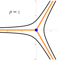
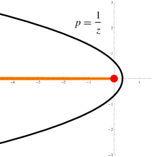
Figure 10: Patterns of WKB lines in $AdS_{3}$, where we choose $\theta=\pi/2$. The two figures illustrate the behavior of WKB lines near zero and simple pole respectively. WKB lines which end on zeros or poles are shown in orange color. Zeros are shown as blue points, while poles are denoted as red points.

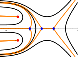
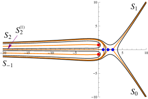
Figure 11: WKB lines in $AdS_{3}$ for the polynomial $p(z)$=${(z-1)(z-2)(z-3)\over(z+i)(z-i)}$, $\theta=\pi/2$. It corresponds to a six-point (${\hat{n}}$=3) form factor with two operators inserted. The second figure plots the WKB lines in a much larger range, which makes it obvious that there are three cusps at infinity.

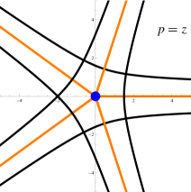
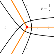
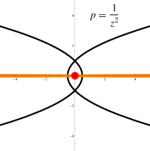
Figure 12: Patterns of WKB lines in $AdS_{5}$, where we choose $\theta=0$. The three figures illustrate the behavior of WKB lines near zero, simple pole and double pole respectively. Zeros are shown as blue points, while poles are denoted as red points. Orange lines are special WKB lines which end on zeros or poles.

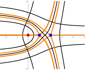
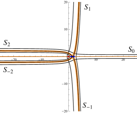
Figure 13: WKB lines in $AdS_{5}$ for the polynomial $p(z)$=${(z-1)(z-2)\over z^{2}}$, $\theta=0$. It corresponds to a four-point form factor. The second figure plots the WKB lines in a much larger range, which makes it obvious that there are four cusps at infinity.

The WKB lines in $AdS_{3}$ have the following structure. For a general point, there is only one WKB line going through. The special points are the zeros and poles. There are three lines ending on each zero, and one line ending on each (simple) pole. These are shown in Figure 10. The full WKB lines for the six-point form factor with two-operator inserted are shown in Figure 11.

The $AdS_{5}$ case corresponds to a $SU(4)$ Hitchin system. The WKB lines have more complicated structures. For a general point, there are two WKB lines going through . There are five lines ending on each zero, three lines ending on each simple pole and two lines ending on each double pole. The WKB patterns are show in Figure 12. The WKB lines for a four-point form factor are given in Figure 13.

One can associate small solutions to the asymptotic WKB lines, as labeled in Figure 11 and 13. Integrals over WKB lines (show as black lines in the figures) that connect different small solutions will provide the WKB approximation for the contraction of small solutions. For Y-functions, the corresponding WKB lines always form a closed contour. Therefore, the WKB approximation of Y functions in the limit of $\zeta\rightarrow 0,\infty$ is given by cycle integrals, which are related to the mass parameters [26]. They are related to the coefficients $a_{i}$ appearing in $P(z)$, and also implicitly related to the shape and periods of Wilson lines.

8 Summary and discussions

In this paper, we study form factors in ${\cal N}=4$ SYM at strong coupling in $AdS_{5}$ and with multi-operator insertions. These are two non-trivial generalizations of the $AdS_{3}$ form factors studied in [36].

The generalization to $AdS_{5}$ involves new technical problems comparing to the $AdS_{3}$ case. The main challenge is how to introduce the truncation conditions with a more complicated $4\times 4$ monodromy matrix, and how to write the system in a gauge invariant form, i.e. in terms of Y-functions. We clarify and solve these problems. The Y-system of three-point case is constructed explicitly, which potentially would have a connection to the strong coupling Higgs-to-3-gluon amplitudes in QCD.

The second generalization to the multi-operator insertion cases provides a more interesting picture and we would like to make a few further comments. The main hope is to provide a new technique to study correlation functions. In doing so, we take an unconventional point of view at strong coupling: to apply the on-shell techniques to compute off-shell observables. Although similar ideas have been studied in the weak coupling side, this point of view seems have not been taken seriously at strong coupling.

According to the picture we proposed, adding one operator corresponds to introducing a new monodromy matrix, which is taken as a condition imposed on small solutions related to null cusps. The techniques developed for amplitudes or null Wilson loops can be applied to the computation of such more general class of observables. We construct the Y-system explicitly for the $AdS_{3}$ case with arbitrary number of operator-insertions. The construction should in principle be generalizable to $AdS_{5}$ based on the prescription of the single-operator result developed in this paper.

The derivation of the Y-system is expected to be applicable for general operators. Different operators would correspond to different kinds of monodromies. The simplest case is for short operators which are dual to light string states as being studied. For them, the monodromy depends only on the momenta of the operators. This is actually very interesting, considering that normally it is hard to study correlation functions with purely light operators at strong coupling besides the perturbative Witten diagram techniques, partially due to the complexity of string vertex operators in $AdS_{5}$ (see some ideas in [73]). In our setup, the vertex operator information is in some sense encoded in the geometry via T-duality, and the problem becomes totally classical. It would also be interesting to construct the monodromy for more general operators, in particular classical solutions such as the GKP string [74].

Although our construction relies on the on-shell structure of the observables, the multi-operator structure should in principle contain all kinds of information in correlation functions. In particular from the general structure of OPE

$${\cal O}_{1}(x)\,{\cal O}_{2}(y)\ =\ \sum_{\alpha}\,c_{12\alpha}\,f(x-y,\partial_{y})\,{\cal O}_{\alpha}(y)\,,$$ (8.1)

an immediate step would be extracting the OPE coefficients by using form factors with two operator insertions and comparing it with form factor with the single operator ${\cal O}_{\alpha}$ in the OPE expansion.

Although our construction of $Y$ system does not rely on an exact knowledge of the string solutions, we do not have an explicit string T-dual picture of a form factor with multi-operator insertions. As discussed in section 7, this should provide a better knowledge for the function $P(z)$. The T-dual picture of short string states was studied recently in [75], where a similar Wilson line picture was obtained. It would be interesting to understand the picture of interacting multi-closed-string states.

While there are lots of studies on correlation functions, we would like to point out particularly [76, 77, 78, 79], where quite similar integrability techniques have been used. However, the detailed physical pictures and the building blocks are quite different. The method in those papers is limited to classical heavy operators (where the $S^{5}$ geometry plays also an important role), while our prescription is focused on short operators (but in principle could be for more general operators). It would be interesting to study the possible connection between the two pictures.

There are interesting algebraic curves appearing in the construction as discussed in Section 7. Similar algebraic curves (the Seiberg-Witten curves) also appear in gauge theories [69]. It would be interesting to study their possible connections. There are also similar spectral curves for classical string solutions such as those studied in [80]. There is an important difference though: while the spectral curve is a curve defined on the spectral parameter $\zeta$-plane, the algebraic curve here is on the worldsheet $z$-plane. On the other hand, in our picture there are close interplays between the two planes. It would be interesting to understand the connection more explicitly.

We would also like to make a few comments on the symmetries. Unlike amplitudes, form factors do not have dual conformal symmetry . However, as we have seen that there is no problem to use integrability to compute strong coupling form factors. Technically this may be understood that through changing of variables, one can bring spacetime quantities to a picture on the worldsheet, where the symmetries are in some sense enhanced and integrability techniques can be applied. It would be very interesting to study its possible correspondence at weak coupling, for example to have a realization of small solution picture at weak coupling, see an interesting proposal along this direction in [81] . In our opinion, it would be the symmetry of the theory rather than the symmetry of observables that plays the most important role.

Finally, let us mention that there are a few technical problems to clarify. While we have obtained the Y-system and considered the WKB approximation, we have not discussed how to find the explicit solutions. The explicit integral form of the Y-system equations are not given. The main complexity is due to the phases of some functions appearing in the equation are outside the physical strip, and extra pole contributions need to be considered. It is also necessary to show how to derive the expression for the area. For the $AdS_{5}$ form factors, a natural expression for the non-trivial free energy part is proposed, while for the multi-operator case a further study is necessary. There are also some issue about the $P(z)$ function of the multi-operator insertion case. These problems are under investigation and we hope to report them in the near future.

Appendix A Hirota and Y-system equations

We start with Cramer s rule:

$$s_{i_{1}}\langle s_{i_{2}},s_{i_{3}},\cdots,s_{i_{k+1}}\rangle-s_{i_{2}}\langle s_{i_{1}},s_{i_{3}},\cdots,s_{i_{k+1}}\rangle+\cdots+(-1)^{k}s_{i_{k+1}}\langle s_{i_{1}},\cdots,s_{i_{k}}\rangle=0\,,$$ (A.1)

where $s_{i}$ is a $k$ dimensional vector and the contraction is defined as

$$\langle s_{1},s_{2},\ldots,s_{k}\rangle\ :=\ \epsilon^{\alpha_{1}\ldots\alpha_{k}}s_{1,\alpha_{1}}\ldots s_{k,\alpha_{k}}\,.$$ (A.2)

Plücker relations can be obtained by contracting the small solutions with another set of small solutions $s_{j_{1}},\cdots,s_{j_{k-1}}$

$$\langle s_{j_{1}},\cdots,s_{j_{k-1}},s_{i_{1}}\rangle\langle s_{i_{2}},s_{i_{3}},\cdots,s_{i_{k+1}}\rangle+\cdots+(-1)^{k}\langle s_{j_{1}},\cdots,s_{j_{k-1}},s_{i_{k+1}}\rangle\langle s_{i_{1}},\cdots,s_{i_{k}}\rangle=0\,.$$ (A.3)

When $k=2$, one gets the Schouten identity

$$\langle s_{i},s_{j}\rangle\langle s_{k},s_{l}\rangle+\langle s_{i},s_{k}\rangle\langle s_{l},s_{j}\rangle+\langle s_{i},s_{l}\rangle\langle s_{j},s_{k}\rangle=0\,.$$ (A.4)

When $k=4$, one obtains useful relations for the $AdS_{5}$ case, such as the Wronskian relation

$$\langle s_{i},s_{j},s_{a},s_{b}\rangle\langle s_{k},s_{l},s_{a},s_{b}\rangle+\langle s_{i},s_{k},s_{a},s_{b}\rangle\langle s_{l},s_{j},s_{a},s_{b}\rangle+\langle s_{i},s_{l},s_{a},s_{b}\rangle\langle s_{j},s_{k},s_{a},s_{b}\rangle=0\,.$$ (A.5)

Below we give the definition of T- and Y-functions, then we apply the above relations to obtain corresponding equations.

A.1 The $AdS_{3}$ case

We use the convention (note it is different from the $AdS_{5}$ case):

$$f^{\pm}\ :=\ f(e^{\pm i{\pi\over 2}}\zeta),\qquad f^{[k]}\ :=\ f(e^{i{k\pi\over 2}}\zeta)\ .$$ (A.6)

In this notation one has from (2.19)

$$\langle s_{i+1},s_{j+1}\rangle\ =\ \langle s_{i},s_{j}\rangle^{[2]}\,.$$ (A.7)

The T-functions are defined as

$$\begin{array}[]{lll}T_{1,2m+1}\ :=\ \langle s_{-m-1},s_{m+1}\rangle,&&T_{1,2m}\ :=\ \langle s_{-m-1},s_{m}\rangle^{+},\\ T_{0,2m}\ :=\ \langle s_{-m-1},s_{-m}\rangle,&&T_{0,2m+1}\ :=\ \langle s_{-m-2},s_{-m-1}\rangle^{+},\\ T_{2,2m}\ :=\ \langle s_{m},s_{m+1}\rangle,&&T_{2,2m+1}\ :=\ \langle s_{m},s_{m+1}\rangle^{+}.\end{array}$$ (A.8)

$T_{1,m}$ is non-zero for $m=1,...,n-1$, and the normalization $\langle s_{0},s_{1}\rangle=1$ corresponds to a gauge choice $T_{0,m}=T_{2,m}=1$.

Using Schouten identity (A.4), one can obtain the so-called Hirota equations

$$T^{+}_{a,m}T^{-}_{a,m}\ =\ T_{a,m-1}T_{a,m+1}+T_{a-1,m}T_{a+1,m}\,,$$ (A.9)

where the indices $a,m$ take integer values.

Hirota equations contain huge gauge redundancies

$$T_{a,m}(\zeta)\ \rightarrow\ \prod_{\alpha,\beta=\pm}g_{\alpha\beta}(e^{{i\pi\over 2}(\alpha a+\beta m)}\zeta)T_{a,m}(\zeta)\,,$$ (A.10)

where $g_{\alpha\beta}(\zeta)$ are four arbitrary functions. Like defining field strength in gauge theory, one can introduce gauge invariant functions, so-called Y-functions

$$Y_{a,m}\ :=\ {T_{a,m-1}T_{a,m+1}\over T_{a-1,m}T_{a+1,m}}\,.$$ (A.11)

The Hirota equations become the equations of Y-functions

$${Y^{+}_{a,m}Y^{-}_{a,m}\over Y_{a-1,m}Y_{a+1,m}}\ =\ {(1+Y_{a,m-1})(1+Y_{a,m+1})\over(1+Y_{a-1,m})(1+Y_{a+1,m})}\,.$$ (A.12)

In the normalization $\langle s_{i},s_{i+1}\rangle=1$ the equations of Y-functions simplify as

$$Y^{+}_{m}Y^{-}_{m}\ =\ (1+Y_{m-1})(1+Y_{m+1})\,,$$ (A.13)

where $Y_{m}:=Y_{1,m}$ .

A.2 The $AdS_{5}$ case

We use the convention:

$$f^{\pm}\ :=\ f(e^{\pm i{\pi\over 4}}\zeta)\,,\qquad f^{[k]}\ :=\ f(e^{i{k\pi\over 4}}\zeta)\,.$$ (A.14)

Useful relations due to the $Z_{4}$ automorphism are

$$\langle s_{j-1},s_{j},s_{k-1},s_{k}\rangle^{[2]}\ =\ \langle s_{j},s_{j+1},s_{k},s_{k+1}\rangle\,,$$ (A.15)

$$\langle s_{k},s_{j-2},s_{j-1},s_{j}\rangle^{[2]}\ =\ \langle s_{k},s_{k+1},s_{k+2},s_{j}\rangle\,.$$ (A.16)

Define the T-functions as

$$T_{0,m}(\zeta)\ :=\ \langle s_{-2},s_{-1},s_{0},s_{1}\rangle^{[-m-1]}\,,$$

$$T_{1,m}(\zeta)\ :=\ \langle s_{-2},s_{-1},s_{0},s_{m+1}\rangle^{[-m]},$$

$$T_{2,m}(\zeta)\ :=\ \langle s_{-1},s_{0},s_{m+1},s_{m+2}\rangle^{[-m-1]}\ ,$$ (A.17)

$$T_{3,m}(\zeta)\ :=\ \langle s_{-1},s_{m},s_{m+1},s_{m+2}\rangle^{[-m]}\ ,$$

$$T_{4,m}(\zeta)\ :=\ \langle s_{m},s_{m+1},s_{m+2},s_{m+3}\rangle^{[-m-1]}\,.$$

Using the Wronskian relation, one obtains the Hirota equations

$$T^{+}_{a,m}T^{-}_{4-a,m}\ =\ T_{4-a,m+1}T_{a,m-1}+T_{a+1,m}T_{a-1,m},\ \ \ a=1,2,3\,.$$ (A.18)

Gauge invariant Y-functions can be defined similarly as

$$Y_{a,m}\ :=\ {T_{a,m+1}T_{4-a,m-1}\over T_{a+1,m}T_{a-1,m}}\,.$$ (A.19)

The Hirota equations become the Y-system equations:

$${Y^{-}_{a,m}Y^{+}_{4-a,m}\over Y_{a+1,m}Y_{a-1,m}}\ =\ {(1+Y_{a,m+1})(1+Y_{4-a,m-1})\over(1+Y_{a+1,m})(1+Y_{a-1,m})},\ \ \ a=1,2,3\ .$$ (A.20)

Appendix B Twistor variables

In this appendix we give a brief review on (momentum) twistor variables, see for example [64, 83]. One technical point we would like to clarify is how to transform twistor variables into Lorentz variables, and vice verse.

We first recall the relation between embedding and Poincaré coordinates

$$X^{\mu}\ =\ {x^{\mu}\over r},\qquad X^{+}\ =\ {1\over r},\qquad X^{-}\ =\ {r^{2}+x^{\mu}x_{\mu}\over r}\,,$$ (B.1)

where ($\eta_{\mu\nu}=(-1,1,1,1)$)

$$-1\ =\ -X^{+}X^{-}+X^{\mu}X_{\mu}\,,\qquad X^{\pm}\ :=\ X^{-1}\pm X^{4}\,.$$ (B.2)

Twistor variables can be understood as in the spinor representation of the embedding $SO(2,4)$ space, which is a $SU(4)$ fundamental representation, denoted by $\lambda$,

$$X_{ab}\ =\ \Gamma^{A}_{ab}\cdot X_{A}=\lambda_{[a}\,\lambda_{b]}\,,\qquad\lambda_{[a}\,\lambda_{b]}\ :=\ \lambda_{a}\lambda_{b}-\lambda_{b}\lambda_{a}\,.$$ (B.3)

With one explicit choice of gamma matrices, one has

$$X_{ab}\ =\ {1\over\sqrt{2}}\,\begin{pmatrix}0&i\,X^{+}&X^{2}+iX^{3}&X^{1}-X^{0}\\ *&0&X^{1}+X^{0}&-X^{2}+iX^{3}\\ *&*&0&i\,X^{-}\\ *&*&*&0\end{pmatrix}\ =\ \lambda_{[a}\,\lambda_{b]}\,.$$ (B.4)

Note that $\det(X)=(X\cdot X)^{2}/4$. Due to the freedom of choosing normalization, twistor variables $\lambda_{i}$ are projective coordinates in ${\rm CP}^{3}$.

Using (B.1) and (B.4), one can obtain the relations between $\lambda_{a}$ and $x^{\mu}$. For example, define

$$x^{\pm}\ =\ x^{1}\pm x^{0}\,,$$ (B.5)

one has the relations

$$x^{-}_{j}\ =\ i\,{X_{j,14}\over X_{j,12}}=i\,{\lambda^{j}_{[1}\,\lambda^{j+1}_{4]}\over\lambda^{j}_{[1}\,\lambda^{j+1}_{2]}}\ ,\qquad x^{+}_{j}\ =\ i\,{X_{j,23}\over X_{j,12}}=i\,{\lambda^{j}_{[2}\,\lambda^{j+1}_{3]}\over\lambda^{j}_{[1}\,\lambda^{j+1}_{2]}}\ .$$ (B.6)

Another description of so-called momentum twistors, which was first introduced at weak coupling [64], is practically more useful . Consider a null Wilson line configuration defined in the momentum space of amplitudes or form factors

$$x_{i+1}-x_{i}\ =\ p_{i}\,,\qquad p_{i}^{2}\ =\ 0\,,\qquad p_{i,\alpha\dot{\alpha}}\ =\ \Lambda_{i,\alpha}\,\tilde{\Lambda}_{i,\dot{\alpha}}\,,$$ (B.7)

where the left and right-hand $SU(2)$ Weyl spinors are denoted by $\Lambda$ and $\tilde{\Lambda}$. We define $x_{ij}:=x_{i}-x_{j}$. The Weyl spinor contractions are defined as

$$\langle i,j\rangle\ :=\ \epsilon^{\alpha\beta}\Lambda_{i,\alpha}\Lambda_{j,\beta}\,,\quad\quad\ \ \,\ \ \qquad[i,j]\ :=\ \epsilon^{\dot{\alpha}\dot{\beta}}\tilde{\Lambda}_{i,\dot{\alpha}}\tilde{\Lambda}_{j,\dot{\beta}}\,,$$ (B.8)

$${\langle i|\,x\,y\,|j\rangle}\ :=\ \Lambda_{i}^{\alpha}\,x_{\alpha\dot{\alpha}}\,y^{\dot{\alpha}\beta}\,\Lambda_{j,\beta}\,,\qquad{\langle i|\,x\,|j]}\ :=\ \Lambda_{i}^{\alpha}\,x_{\alpha\dot{\beta}}\,\tilde{\Lambda}_{j}^{\dot{\beta}}\,.$$ (B.9)

The momentum twistors can be explicitly defined as follows

$$\lambda_{j}\ =\ \big{(}\Lambda_{j,\alpha},\,\mu_{j,\dot{\alpha}}\big{)},\qquad\mu_{j,\dot{\alpha}}\ :=\ -i\,(x_{j}\cdot\Lambda_{j})_{\dot{\alpha}}\ =\ -i\,\epsilon^{\alpha\beta}x_{j,\alpha\dot{\alpha}}\Lambda_{j,\beta}\,.$$ (B.10)

Note that also $\mu_{j,\dot{\alpha}}=-i\,(x_{j+1}\cdot\Lambda_{j})_{\dot{\alpha}}$ . The contraction of twistors is defined as

$$\langle\lambda_{i},\lambda_{j},\lambda_{k},\lambda_{l}\rangle\ :=\ \epsilon^{abcd}\lambda_{i,a}\lambda_{j,b}\lambda_{k,c}\lambda_{l,d}\,,\qquad a=(\alpha,\dot{\alpha})\ .$$ (B.11)

The geometric picture of twistor space is that, each spacetime point corresponds to a line in twistor space determined by two twistor variable, $x_{i}\sim X_{i}\sim\lambda_{i-1}\wedge\lambda_{i}$. If two spacetime points are null separated, the corresponding two lines in twistor space intersect with each other. This is obvious in the above definition since null-separated $x_{i}$ and $x_{i+1}$ both contain $\lambda_{i}$.

To write the contractions of twistor variables in terms of Lorentz coordinates, one practically very useful formula is [83]

$${\langle i|\,x_{i,j}\,x_{j,k}\,|k\rangle}\ =\ {\langle\lambda_{i},\lambda_{j-1},\lambda_{j},\lambda_{k}\rangle\over\langle j-1,j\rangle}\,.$$ (B.12)

For example, using (B.12) it is easy to obtain the relation

$$x_{i,j}^{2}\ =\ {\langle\lambda_{i-1},\lambda_{i},\lambda_{j-1},\lambda_{j}\rangle\over\langle i-1,i\rangle\langle j-1,j\rangle}\,.$$ (B.13)

Furthermore, any normalization independent expression of twistor contractions can be written in terms of Lorentz variables. For example, for the ratio variables appearing in form factors, one has

$${\langle\lambda_{1},\lambda_{2},\lambda_{3},\hat{\Omega}\lambda_{4}\rangle\over\langle\lambda_{1},\lambda_{2},\lambda_{3},\lambda_{4}\rangle}\ =\ {\langle\lambda_{1},\lambda_{2},\lambda_{3},\lambda_{4+n}\rangle\over b_{4}\,\langle\lambda_{1},\lambda_{2},\lambda_{3},\lambda_{4}\rangle}\ =\ {\langle 1|p_{2}\,(q+p_{3})|4\rangle\over\langle 1|p_{2}\,p_{3}|4\rangle}\,,$$ (B.14)

$${\langle\hat{\Omega}\,\lambda_{1},\lambda_{2},\lambda_{3},\lambda_{4}\rangle\over\langle\lambda_{1},\lambda_{2},\lambda_{3},\lambda_{4}\rangle}\ =\ {\langle\lambda_{n+1},\lambda_{2},\lambda_{3},\lambda_{4}\rangle\over b_{1}\,\langle\lambda_{1},\lambda_{2},\lambda_{3},\lambda_{4}\rangle}\ =\ {\langle 1|(-q+p_{12})\,p_{3}|4\rangle\over\langle 1|p_{12}\,p_{3}|4\rangle}\,,$$ (B.15)

where we also use the relation (4.55) $\lambda_{i+n}=b_{i}\,\hat{\Omega}\,\lambda_{i}$.

Appendix C Monodromy with a different basis

In this section we briefly explain the monodromy defined in a different basis of small solutions, in particular how $\overline{\Omega}$ is related to $\Omega$.

First recall the definition of the monodromy

$$\begin{pmatrix}s_{1}\\ s_{0}\\ s_{-1}\\ s_{-2}\end{pmatrix}(ze^{2\pi i},\zeta)=\Omega^{-1}(\zeta)\begin{pmatrix}s_{1}\\ s_{0}\\ s_{-1}\\ s_{-2}\end{pmatrix}(z,\zeta)\,,\ \ \begin{pmatrix}s_{2}\\ s_{1}\\ s_{0}\\ s_{-1}\end{pmatrix}(ze^{2\pi i},\zeta)=(\overline{\Omega}^{[2]})^{-1}(\zeta)\begin{pmatrix}s_{2}\\ s_{1}\\ s_{0}\\ s_{-1}\end{pmatrix}(z,\zeta)\,,$$ (C.1)

and

$$\begin{pmatrix}s_{n+1},s_{n},s_{n-1},s_{n-2}\end{pmatrix}^{T}(z,\zeta) = {\cal B}^{-1}(\zeta)\begin{pmatrix}s_{1},s_{0},s_{-1},s_{-2}\end{pmatrix}^{T}(ze^{-2\pi i},\zeta)\,,$$

$$\begin{pmatrix}s_{n+2},s_{n+1},s_{n},s_{n-1}\end{pmatrix}^{T}(z,\zeta) = ({\overline{\cal B}}^{[2]})^{-1}(\zeta)\begin{pmatrix}s_{2},s_{1},s_{0},s_{-1}\end{pmatrix}^{T}(ze^{-2\pi i},\zeta)\,,$$ (C.2)

where using the relations of (2.20), the proportionality constants are given by a single $B$ function

$${\cal B}^{-1} = {\rm diag}\big{\{}B,(B^{[2]})^{-1},B^{[-4]},(B^{[-2]})^{-1}\big{\}}\,,$$

$${\overline{\cal B}}^{-1} = {\rm diag}\big{\{}(B^{[4]})^{-1},B^{[-2]},B^{-1},B^{[2]}\big{\}}\,.$$ (C.3)

One can expand $s_{-2}$ in terms of $\{s_{-1},s_{0},s_{1},s_{2}\}$, then one gets

$$s_{-2}\ =\ T_{1,1}^{[-1]}\,s_{-1}-T_{2,1}\,s_{0}+T_{1,1}^{[1]}\,s_{1}-s_{2}\,.$$ (C.4)

Similarly for $s_{n-2}$ one has the expansion

$$s_{n-2}\,=\,\langle s_{n-2},s_{n},s_{n+1},s_{n+2}\rangle\,s_{n-1}-T_{2,1}^{[2n-4]}\,s_{n}+\langle s_{n-2},s_{n-1},s_{n},s_{n+2}\rangle\,s_{n+1}-s_{n+2}\,,$$ (C.5)

where the other two contractions are $T_{1,1}$ or $T_{3,1}$ depending on whether $n$ is even or odd.

By introducing

$$M = \begin{pmatrix}0&1&0&0\\ 0&0&1&0\\ 0&0&0&1\\ -1&T_{1,1}^{[1]}&-T_{2,1}&T_{1,1}^{[-1]}\end{pmatrix},\$$ (C.6)

$$M^{\prime} = \begin{pmatrix}0&1&0&0\\ 0&0&1&0\\ 0&0&0&1\\ -1&\langle s_{n-2}s_{n-1}s_{n}s_{n+2}\rangle&-T_{2,1}^{[2n-4]}&\langle s_{n-2}s_{n}s_{n+1}s_{n+2}\rangle\end{pmatrix},$$ (C.7)

one can obtain

$$(\overline{\Omega}^{[2]})\ =\ \overline{B}^{[2]}\,M^{\prime-1}\,B^{-1}\,\Omega\,M\,.$$ (C.8)

References

- [1] Z. Bern, L. J. Dixon and D. A. Kosower, “N=4 super-Yang-Mills theory, QCD and collider physics,” Comptes Rendus Physique 5, 955 (2004) [hep-th/0410021].
- [2] A. V. Kotikov, L. N. Lipatov, A. I. Onishchenko and V. N. Velizhanin, “Three loop universal anomalous dimension of the Wilson operators in N=4 SUSY Yang-Mills model,” Phys. Lett. B 595, 521 (2004) [Erratum-ibid. B 632, 754 (2006)] [hep-th/0404092].
- [3] J. M. Maldacena, “The Large N limit of superconformal field theories and supergravity,” Adv. Theor. Math. Phys. 2, 231 (1998) [hep-th/9711200].
- [4] S. S. Gubser, I. R. Klebanov and A. M. Polyakov, “Gauge theory correlators from noncritical string theory,” Phys. Lett. B 428, 105 (1998) [hep-th/9802109].
- [5] E. Witten, “Anti-de Sitter space and holography,” Adv. Theor. Math. Phys. 2, 253 (1998) [hep-th/9802150].
- [6] N. Beisert, B. Eden and M. Staudacher, “Transcendentality and Crossing,” J. Stat. Mech. 0701, P01021 (2007) [hep-th/0610251].
- [7] N. Gromov, V. Kazakov and P. Vieira, “Exact Spectrum of Anomalous Dimensions of Planar N=4 Supersymmetric Yang-Mills Theory,” Phys. Rev. Lett. 103, 131601 (2009) [arXiv:0901.3753 [hep-th]].
- [8] D. Bombardelli, D. Fioravanti and R. Tateo, “Thermodynamic Bethe Ansatz for planar AdS/CFT: A Proposal,” J. Phys. A 42, 375401 (2009) [arXiv:0902.3930 [hep-th]].
- [9] G. Arutyunov and S. Frolov, “Thermodynamic Bethe Ansatz for the AdS(5) x S(5) Mirror Model,” JHEP 0905, 068 (2009) [arXiv:0903.0141 [hep-th]].
- [10] N. Gromov, V. Kazakov, S. Leurent and D. Volin, “Solving the AdS/CFT Y-system,” JHEP 1207, 023 (2012) [arXiv:1110.0562 [hep-th]].
- [11] G. Mandal, N. V. Suryanarayana and S. R. Wadia, “Aspects of semiclassical strings in AdS(5),” Phys. Lett. B 543, 81 (2002) [hep-th/0206103].
- [12] J. A. Minahan and K. Zarembo, “The Bethe ansatz for N=4 superYang-Mills,” JHEP 0303, 013 (2003) [hep-th/0212208].
- [13] I. Bena, J. Polchinski and R. Roiban, “Hidden symmetries of the AdS(5) x S**5 superstring,” Phys. Rev. D 69, 046002 (2004) [hep-th/0305116].
- [14] N. Beisert, C. Ahn, L. F. Alday, Z. Bajnok, J. M. Drummond, L. Freyhult, N. Gromov and R. A. Janik et al., “Review of AdS/CFT Integrability: An Overview,” Lett. Math. Phys. 99, 3 (2012) [arXiv:1012.3982 [hep-th]].
- [15] L. F. Alday and J. M. Maldacena, “Gluon scattering amplitudes at strong coupling,” JHEP 0706, 064 (2007) [arXiv:0705.0303 [hep-th]].
- [16] J. M. Drummond, G. P. Korchemsky and E. Sokatchev, “Conformal properties of four-gluon planar amplitudes and Wilson loops,” Nucl. Phys. B 795, 385 (2008) [arXiv:0707.0243 [hep-th]].
- [17] A. Brandhuber, P. Heslop and G. Travaglini, “MHV amplitudes in N=4 super Yang-Mills and Wilson loops,” Nucl. Phys. B 794, 231 (2008) [arXiv:0707.1153 [hep-th]].
- [18] J. M. Drummond, J. Henn, G. P. Korchemsky and E. Sokatchev, “Conformal Ward identities for Wilson loops and a test of the duality with gluon amplitudes,” Nucl. Phys. B 826, 337 (2010) [arXiv:0712.1223 [hep-th]].
- [19] J. M. Drummond, J. M. Henn and J. Plefka, “Yangian symmetry of scattering amplitudes in N=4 super Yang-Mills theory,” JHEP 0905, 046 (2009) [arXiv:0902.2987 [hep-th]].
- [20] L. J. Mason and D. Skinner, “The Complete Planar S-matrix of N=4 SYM as a Wilson Loop in Twistor Space,” JHEP 1012, 018 (2010) [arXiv:1009.2225 [hep-th]].
- [21] S. Caron-Huot and S. He, “Jumpstarting the All-Loop S-Matrix of Planar N=4 Super Yang-Mills,” JHEP 1207, 174 (2012) [arXiv:1112.1060 [hep-th]].
- [22] L. F. Alday, B. Eden, G. P. Korchemsky, J. Maldacena and E. Sokatchev, “From correlation functions to Wilson loops,” JHEP 1109, 123 (2011) [arXiv:1007.3243 [hep-th]].
- [23] B. Eden, G. P. Korchemsky and E. Sokatchev, “From correlation functions to scattering amplitudes,” JHEP 1112, 002 (2011) [arXiv:1007.3246 [hep-th]].
- [24] L. F. Alday and J. Maldacena, “Null polygonal Wilson loops and minimal surfaces in Anti-de-Sitter space,” JHEP 0911, 082 (2009) [arXiv:0904.0663 [hep-th]].
- [25] L. F. Alday, D. Gaiotto and J. Maldacena, “Thermodynamic Bubble Ansatz,” JHEP 1109, 032 (2011) [arXiv:0911.4708 [hep-th]].
- [26] L. F. Alday, J. Maldacena, A. Sever and P. Vieira, “Y-system for Scattering Amplitudes,” J. Phys. A A 43, 485401 (2010) [arXiv:1002.2459 [hep-th]].
- [27] G. Yang, “Scattering amplitudes at strong coupling for 4K gluons,” JHEP 1012, 082 (2010) [arXiv:1004.3983 [hep-th]]. “A simple collinear limit of scattering amplitudes at strong coupling,” JHEP 1103, 087 (2011) [arXiv:1006.3306 [hep-th]].
- [28] J. Bartels, J. Kotanski and V. Schomerus, “Excited Hexagon Wilson Loops for Strongly Coupled N=4 SYM,” JHEP 1101, 096 (2011) [arXiv:1009.3938 [hep-th]].
- [29] J. Bartels, V. Schomerus and M. Sprenger, “Multi-Regge Limit of the n-Gluon Bubble Ansatz,” JHEP 1211, 145 (2012) [arXiv:1207.4204 [hep-th]].
- [30] Y. Hatsuda, K. Ito, K. Sakai and Y. Satoh, “Six-point gluon scattering amplitudes from -symmetric integrable model,” JHEP 1009, 064 (2010) [arXiv:1005.4487 [hep-th]].
- [31] Y. Hatsuda, K. Ito and Y. Satoh, “Null-polygonal minimal surfaces in from perturbed W minimal models,” arXiv:1211.6225 [hep-th].
- [32] V. A. Kazakov, A. Marshakov, J. A. Minahan and K. Zarembo, “Classical/quantum integrability in AdS/CFT,” JHEP 0405, 024 (2004) [hep-th/0402207].
- [33] G. Arutyunov, S. Frolov and M. Staudacher, “Bethe ansatz for quantum strings,” JHEP 0410, 016 (2004) [hep-th/0406256].
- [34] J. Polchinski and L. Susskind, “String theory and the size of hadrons,” hep-th/0112204.
- [35] L. F. Alday and J. Maldacena, “Comments on gluon scattering amplitudes via AdS/CFT,” JHEP 0711, 068 (2007) [arXiv:0710.1060 [hep-th]].
- [36] J. Maldacena and A. Zhiboedov, “Form factors at strong coupling via a Y-system,” JHEP 1011, 104 (2010) [arXiv:1009.1139 [hep-th]].
- [37] W. L. van Neerven, “Infrared Behavior Of On-shell Form-factors In A N=4 Supersymmetric Yang-mills Field Theory,” Z. Phys. C 30, 595 (1986).
- [38] A. Brandhuber, B. Spence, G. Travaglini and G. Yang, “Form Factors in N=4 Super Yang-Mills and Periodic Wilson Loops,” JHEP 1101, 134 (2011) [arXiv:1011.1899 [hep-th]].
- [39] L. V. Bork, D. I. Kazakov and G. S. Vartanov, “On form factors in N=4 SYM,” JHEP 1102, 063 (2011) [arXiv:1011.2440 [hep-th]].
- [40] A. Brandhuber, O. Gurdogan, R. Mooney, G. Travaglini and G. Yang, “Harmony of Super Form Factors,” JHEP 1110, 046 (2011) [arXiv:1107.5067 [hep-th]].
- [41] L. V. Bork, D. I. Kazakov and G. S. Vartanov, “On MHV Form Factors in Superspace for N=4 SYM Theory,” JHEP 1110, 133 (2011) [arXiv:1107.5551 [hep-th]].
- [42] T. Gehrmann, J. M. Henn and T. Huber, “The three-loop form factor in N=4 super Yang-Mills,” JHEP 1203, 101 (2012) [arXiv:1112.4524 [hep-th]].
- [43] A. Brandhuber, G. Travaglini and G. Yang, “Analytic two-loop form factors in N=4 SYM,” JHEP 1205, 082 (2012) [arXiv:1201.4170 [hep-th]].
- [44] T. Gehrmann, M. Jaquier, E. W. N. Glover and A. Koukoutsakis, “Two-Loop QCD Corrections to the Helicity Amplitudes for 3 partons,” JHEP 1202, 056 (2012) [arXiv:1112.3554 [hep-ph]].
- [45] R. H. Boels, B. A. Kniehl, O. V. Tarasov and G. Yang, “Color-kinematic Duality for Form Factors,” JHEP 1302, 063 (2013) [arXiv:1211.7028 [hep-th]].
- [46] O. T. Engelund and R. Roiban, “Correlation functions of local composite operators from generalized unitarity,” arXiv:1209.0227 [hep-th].
- [47] D. J. Gross and P. F. Mende, “String Theory Beyond the Planck Scale,” Nucl. Phys. B 303, 407 (1988).
- [48] R. Kallosh and A. A. Tseytlin, “Simplifying superstring action on AdS(5) x S**5,” JHEP 9810, 016 (1998) [hep-th/9808088].
- [49] T. H. Buscher, “A Symmetry of the String Background Field Equations,” Phys. Lett. B 194, 59 (1987).
- [50] N. Berkovits and J. Maldacena, “Fermionic T-Duality, Dual Superconformal Symmetry, and the Amplitude/Wilson Loop Connection,” JHEP 0809, 062 (2008) [arXiv:0807.3196 [hep-th]].
- [51] N. Beisert, R. Ricci, A. A. Tseytlin and M. Wolf, “Dual Superconformal Symmetry from AdS(5) x S**5 Superstring Integrability,” Phys. Rev. D 78, 126004 (2008) [arXiv:0807.3228 [hep-th]].
- [52] J. M. Maldacena, “Wilson loops in large N field theories,” Phys. Rev. Lett. 80, 4859 (1998) [hep-th/9803002].
- [53] S. J. Rey and J. T. Yee, “Macroscopic strings as heavy quarks in large N gauge theory and anti-de Sitter supergravity,” Eur. Phys. J. C 22, 379 (2001) [hep-th/9803001].
- [54] L. F. Alday, E. I. Buchbinder and A. A. Tseytlin, “Correlation function of null polygonal Wilson loops with local operators,” JHEP 1109, 034 (2011) [arXiv:1107.5702 [hep-th]].
- [55] S. Frolov and A. A. Tseytlin, “Semiclassical quantization of rotating superstring in AdS(5) x S**5,” JHEP 0206, 007 (2002) [hep-th/0204226].
- [56] M. Kruczenski, R. Roiban, A. Tirziu and A. A. Tseytlin, “Strong-coupling expansion of cusp anomaly and gluon amplitudes from quantum open strings in AdS(5) x S**5,” Nucl. Phys. B 791, 93 (2008) [arXiv:0707.4254 [hep-th]].
- [57] C. Anastasiou, Z. Bern, L. J. Dixon, D. A. Kosower, Planar amplitudes in maximally supersymmetric Yang-Mills theory, Phys. Rev. Lett. 91, 251602 (2003), arXiv:hep-th/0309040.
- [58] Z. Bern, L. J. Dixon and V. A. Smirnov, Iteration of planar amplitudes in maximally supersymmetric Yang-Mills theory at three loops and beyond, Phys. Rev. D 72 (2005) 085001 [arXiv:hep-th/0505205].
- [59] N. Berkovits, “Super Poincare covariant quantization of the superstring,” JHEP 0004, 018 (2000) [hep-th/0001035].
- [60] H. J. De Vega and N. G. Sanchez, “Exact integrability of strings in D-Dimensional De Sitter space-time,” Phys. Rev. D 47, 3394 (1993).
- [61] A. Jevicki, K. Jin, C. Kalousios and A. Volovich, “Generating AdS String Solutions,” JHEP 0803, 032 (2008) [arXiv:0712.1193 [hep-th]].
- [62] H. Dorn, G. Jorjadze and S. Wuttke, “On spacelike and timelike minimal surfaces in AdS(n),” JHEP 0905, 048 (2009) [arXiv:0903.0977 [hep-th]].
- [63] K. Pohlmeyer, “Integrable Hamiltonian Systems And Interactions Through Quadratic Constraints,” Commun. Math. Phys. 46, 207 (1976).
- [64] A. Hodges, “Eliminating spurious poles from gauge-theoretic amplitudes,” arXiv:0905.1473 [hep-th].
- [65] J. Schwarz, “Opening lecture of Strings 2012”, http://wwwth.mpp.mpg.de/members/strings/strings2012/strings_files/program/Talks/Monday/Schwarz.pdf.
- [66] C. N. Yang and C. P. Yang, “Thermodynamics of one-dimensional system of bosons with repulsive delta function interaction,” J. Math. Phys. 10, 1115 (1969).
- [67] A. B. Zamolodchikov, “Thermodynamic Bethe Ansatz In Relativistic Models. Scaling Three State Potts And Lee-yang Models,” Nucl. Phys. B 342, 695 (1990).
- [68] L. F. Alday, D. Gaiotto, J. Maldacena, A. Sever and P. Vieira, “An Operator Product Expansion for Polygonal null Wilson Loops,” JHEP 1104, 088 (2011) [arXiv:1006.2788 [hep-th]].
- [69] D. Gaiotto, G. W. Moore and A. Neitzke, “Wall-crossing, Hitchin Systems, and the WKB Approximation,” arXiv:0907.3987 [hep-th].
- [70] A. V. Zhiboedov, “Form factors in theories with gravity duals,” Nucl. Phys. Proc. Suppl. 216, 276 (2011).
- [71] A. B. Goncharov, M. Spradlin, C. Vergu and A. Volovich, “Classical Polylogarithms for Amplitudes and Wilson Loops,” Phys. Rev. Lett. 105, 151605 (2010) [arXiv:1006.5703 [hep-th]].
- [72] L. J. Dixon, J. M. Drummond and J. M. Henn, “Bootstrapping the three-loop hexagon,” JHEP 1111, 023 (2011) [arXiv:1108.4461 [hep-th]].
- [73] J. A. Minahan, “Holographic three-point functions for short operators,” JHEP 1207, 187 (2012) [arXiv:1206.3129 [hep-th]].
- [74] S. S. Gubser, I. R. Klebanov and A. M. Polyakov, “A Semiclassical limit of the gauge/string correspondence,” Nucl. Phys. B 636, 99 (2002) [hep-th/0204051].
- [75] M. Kruczenski and A. A. Tseytlin, “Wilson loops T-dual to Short Strings,” arXiv:1212.4886 [hep-th].
- [76] R. A. Janik and A. Wereszczynski, “Correlation functions of three heavy operators: The AdS contribution,” JHEP 1112, 095 (2011) [arXiv:1109.6262 [hep-th]].
- [77] Y. Kazama and S. Komatsu, “On holographic three point functions for GKP strings from integrability,” JHEP 1201, 110 (2012) [Erratum-ibid. 1206, 150 (2012)] [arXiv:1110.3949 [hep-th]].
- [78] Y. Kazama and S. Komatsu, “Wave functions and correlation functions for GKP strings from integrability,” JHEP 1209, 022 (2012) [arXiv:1205.6060 [hep-th]].
- [79] J. Caetano and J. Toledo, “-Systems for Correlation Functions,” arXiv:1208.4548 [hep-th].
- [80] R. A. Janik and P. Laskos-Grabowski, “Surprises in the AdS algebraic curve constructions: Wilson loops and correlation functions,” Nucl. Phys. B 861, 361 (2012) [arXiv:1203.4246 [hep-th]].
- [81] A. Sever, P. Vieira and T. Wang, “From Polygon Wilson Loops to Spin Chains and Back,” JHEP 1212, 065 (2012) [arXiv:1208.0841 [hep-th]].
- [82] L. Ferro, T. Lukowski, C. Meneghelli, J. Plefka and M. Staudacher, “Harmonic R-matrices for Scattering Amplitudes and Spectral Regularization,” arXiv:1212.0850 [hep-th].
- [83] L. Mason and D. Skinner, “Dual Superconformal Invariance, Momentum Twistors and Grassmannians,” JHEP 0911, 045 (2009) [arXiv:0909.0250 [hep-th]].