Modeling US housing prices by spatial dynamic structural equation models

Abstract

This article proposes a spatial dynamic structural equation model for the analysis of housing prices at the State level in the USA. The study contributes to the existing literature by extending the use of dynamic factor models to the econometric analysis of multivariate lattice data. One of the main advantages of our model formulation is that by modeling the spatial variation via spatially structured factor loadings, we entertain the possibility of identifying similarity “regions” that share common time series components. The factor loadings are modeled as conditionally independent multivariate Gaussian Markov Random Fields, while the common components are modeled by latent dynamic factors. The general model is proposed in a state-space formulation where both stationary and nonstationary autoregressive distributed-lag processes for the latent factors are considered. For the latent factors which exhibit a common trend, and hence are cointegrated, an error correction specification of the (vector) autoregressive distributed-lag process is proposed. Full probabilistic inference for the model parameters is facilitated by adapting standard Markov chain Monte Carlo (MCMC) algorithms for dynamic linear models to our model formulation. The fit of the model is discussed for a data set of 48 States for which we model the relationship between housing prices and the macroeconomy, using State level unemployment and per capita personal income.

, and

1 Introduction

This paper is concerned with the modeling of housing prices at the State level in the US. Housing is a massive factor in people’s consumption. For industrialized nations, for example, it is the biggest component in the basket of goods used for calculating the consumer price index. Also, the Bureau of Labor Statistics has estimated in 2010 that about 24 percent of the total consumption of American home owners goes toward housing. Hence, housing is big enough to leave a sizable footprint on the economy in general.

In the generic sense, housing is also an important social institution in our society. Not only does housing play a major role in any nation’s economy, but it also provides people with the social values of shelter, security, independence, privacy and amenity. The state of the current economy and recent events in the housing sector have thus led to increased attention on the role of the housing sector in the economy as a whole.

Economists have studied the relationship between the housing sector and the macroeconomy since the 1970s. Several socio-economic variables and/or real estate characteristics are traditionally considered to have an impact on housing prices and several studies have thus been dedicated to the determination of fundamental factors explaining US housing price variations. Our primary purpose here is not to comprehensively examine all these variables. In fact, there is no single generally agreed upon set of variables used in testing models of housing prices in the literature. For a complete discussion on this point see, for example, Malpezzi (1999), Capozza et al. (2002) and Gallin (2008). It is thus beyond the scope of this paper to discuss the possible roles played by all fundamental factors in explaining the variation of housing prices. Hence, for simplicity, we only examine here the extent to which these prices are driven by the real per capita disposable income and the unemployment rate.

1.1 The data: A brief description

The data analyzed in this paper are from the St. Louis Federal Reserve Bank database and the Bureau of Labor Statistics and consist of quarterly time series on $48$ States (excluding Alaska and Hawaii) from 1984 (first quarter) to 2011 (fourth quarter). Figure 1 shows the time series of the real housing price index for the 48 United States grouped in the eight Bureau of Economic Analysis (BEA) regions. The time series are expressed in a logarithmic scale—see Section 8 for a complete description of the data set.

Figure 1: Time series of the log-transformed real housing price index. The 48 United States are grouped in the eight Bureau of Economic Analysis (BEA) regions.

Figure 1 shows that there are interesting dynamic structures in the time series and that periodic patterns and common trend components are consistent features of the housing market. Specifically, it appears that housing prices have been rising rapidly. Since 1995 we have estimated that, on average, real housing prices have increased about 36 percent, roughly double the increase of previous housing price booms observed in the late 1980s. Moreover, we notice that housing prices continued to rise strongly during the 2001 recession and that the process of the housing price boom, which some have interpreted as a bubble, started in 1998, accelerated during the period 2003–2006 and burst in 2007. The prices have then been falling sharply over all the country.

The possibility of modeling all these dynamic features, as well as to obtain accurate housing price forecasts, is important for prospective homeowners, investors, appraisers and other real estate market participants, such as mortgage lenders and insurers.

Table 1: Average of correlation coefficients within and between regions first difference log of real housing prices. BEA regions: New England (NE), Mideast (ME), Great Lakes (GL), Plains (PL), Southeast (SE), Southwest (SW), Rocky Mountain (RM), Far West (FW)

	NE	ME	GL	PL	SE	SW	RM	FW
NE	0.80	–	–	–	–	–	–	–
ME	0.72	0.74	–	–	–	–	–	–
GL	0.47	0.48	0.63	–	–	–	–	–
PL	0.23	0.25	0.35	0.50	–	–	–	–
SE	0.35	0.40	0.48	0.36	0.45	–	–	–
SW	0.24	0.29	0.35	0.42	0.42	0.47	–	–
RM	0.10	0.17	0.30	0.46	0.37	0.48	0.50	–
FW	0.33	0.46	0.42	0.34	0.37	0.40	0.41	0.50

The way in which housing prices spread out to surrounding locations over time are also of interest in the real estate literature. The co-movements shown by the time series within BEA regions suggest the presence of spatial correlation. As stated in Holly, Pesaran and Yamagata (2010), it is possible that States that are contiguous may influence each other’s housing prices. In fact, high prices in metropolitan areas may persuade people to commute from neighboring States. Labour mobility is quite high in the USA and lower housing prices may provide an incentive to migrate. Another possible source of cross-sectional dependence would be due to economy-wide common shocks that affect all cross section units. Changes in interest rates, oil prices and technology are examples of such common shocks that may affect housing prices, although with different degrees across States.

To explore the existence of spatial interactions, using data on the growth of real housing prices, Table 1 shows the simple correlation coefficients between each State, within and between correlations for the $8$ BEA regions. The diagonal elements show the within region average correlation coefficients, while the off-diagonal elements give the between region correlation coefficients. Apart from the States of the Southeast, which are more correlated on average with the States of the Great Lakes than among themselves, the within region correlation is larger than the between region correlation. In general, on average, the correlations decline with distance, but it is interesting to note the quite high correlations between the East and West regions, that is, for States belonging to the Mideast and Far West regions. In general, there is more evidence in the raw data of a possible spatial pattern in real housing prices than in real incomes and unemployment rate.

1.2 Related literature and the proposed model

Modeling the spatio-temporal variability of housing prices has enjoyed widespread popularity in the last years. In order to obtain a high degree of accuracy in the results, the analysis of housing prices across US States requires the definition of a general and flexible econometric model where the temporal and cross-sectional dependencies must be accommodated. Several efforts have been made to develop spatio-temporal models but there is no single approach which can be considered uniformly as being the most appropriate. For example, time series models have become increasingly sophisticated in their treatment of dynamics and trends over time, including the application of unit roots and cointegration techniques [Giussani and Hadjimatheou (1991), Meen (2001), Muellbauer and Murphy (1997)]. However, traditional approaches, such as those based on standard vector autoregression analysis (VAR), do not allow for a direct modeling of locational spillovers and are thus not consistent with the “ripple effect” theory [Meen (1999)]. A spatial adaptation of VARs, denoted as SpVAR models, explicitly considers the potential impacts of economic events in neighboring States and has been discussed in Kuethe and Pede (2011). The SpVAR is a specific version of the Spatio-Temporal Auto-Regressive Moving Average—(STARMA)—model introduced by Pfeifer and Deutsch (1980) where the linear dependencies are lagged in both space and time. Since STARMAs are an extension of the ARMA class of models [Box, Jenkins and Reinsel (1994)], they are particularly useful to produce temporal forecasts of the variable of interest. However, the STARMA specification also suffers from some disadvantages. First, because of the amount of computational effort required, STARMAs are in general only suitable for modeling data which are dense in time and sparse in space. For example, in Kuethe and Pede (2011) the analysis is only limited to $11$ States (i.e., West Region). Secondly, the understanding of co-movements among US State housing prices (and other involved variables) is difficult when the number of the States is large. Knowledge of this covariation is required both to academics seeking to explain the economic nature and sources of variation and to practitioners involved in the development of trading strategies. Thirdly, as argued by Anselin [(1988), pages 11–14], the STARMA class does not offer a fully adequate modeling of the spatial dependence and heterogeneity of observations. The lack of an adequate treatment of a simultaneous (instantaneous) spatial dependence is also the main point of criticism raised by Cressie [(1993), page 450] to the STARMA methodology. In fact, in its standard specification, STARMA implicitly assumes that, conditional on past observations, the process is uncorrelated across space. This is undoubtedly a major shortcoming, since many observed series, as noted, for example, by Pfeifer and Deutsch (1981), show considerable contemporaneous correlation even after conditioning on the past history of the process. When the contemporaneous correlation is considered by the model, the observations become a nonlinear transformation of the innovations and, as a result, maximum likelihood estimation becomes much more difficult [Elhorst (2001), Di Giacinto et al. (2005)].

Seemingly Unrelated Regression (SUR) and error correction panel data models [see, e.g., Meen (2001), Cameron, Muellbauer and Murphy (2006)] have also been largely used with spatial and time effects to investigate the evolution of housing prices. Apart from their rather complex structure, as STARMAs, these models are not suitable when the number of regions is relatively large. In fact, the application of an unrestricted SURE-GLS approach to large $N$ (cross section dimension) and $T$ (time series dimension) panels involves nuisance parameters that increase at a quadratic rate as the cross section dimension of the panel is allowed to rise [Pesaran (2006)].

Recent research has found that in a data rich environment, dimension reduction in the form of factors is useful for exploratory analysis, prediction and policy analysis. Factor analysis assumes that the cross dependence can be characterized by a finite number of unobserved common factors, possibly due to economy-wide shocks that affect all States, albeit with different intensities. Thus, strong co-movement and high correlation among the series suggest that both observable and unobservable factors must be at place. The effects of common shocks on housing prices have been taken in consideration in van Dijk et al. (2011) and Holly, Pesaran and Yamagata (2010) by making use of the common correlated effects estimator [CCE, Pesaran (2006)] which controls for heterogeneity and spatial dependence. In these studies, the authors develop a panel data model where fixed mean effects, cointegration, cross-equation correlations and latent factors are considered. Furthermore, they show that by approximating the linear combinations of the unobserved factors by cross section averages of the dependent and explanatory variables, and by running standard panel regressions augmented with these cross section averages, spatial dependency can be eliminated.

Differently from these authors, we approach the analysis from the perspective of recent developments of dynamic factor models in the literature of spatio-temporal processes. We assume that the observed process can be modeled by a temporally dynamic and spatially descriptive model, hereafter referred to as the spatial dynamic structural equation model—SD-SEM. There are some important differences between our approach and the one discussed by Holly, Pesaran and Yamagata (2010) and van Dijk et al. (2011). Firstly, differently from these authors, we do not use cross section averages to eliminate cross-sectional dependencies. Instead, our model formulation exploits the spatio-temporal nature of the data and explicitly defines a nonseparable spatio-temporal covariance structure of the multivariate process. Secondly, because of the high dimensionality of the data, dimension reduction is important and we suggest modeling the temporal relationship between dependent and regressor variables in a latent space. The observed processes are thus described by a potentially small set of common dynamic latent factors. For all possible model candidates which may be specified, we use a multivariate autoregressive distributed-lag specification for these latent processes and, to account for situations in which two or more latent factors appear to exhibit a common trend, their cointegrating relationship is considered. Thirdly, by modeling the spatial variation via spatially structured factor loadings, we entertain the possibility of identifying clusters of States that share common time series components. This is one of the main advantages of our model formulation. Lastly, the model naturally allows for producing temporal and spatial predictions of the variables of interest. Note that although spatial interpolation is not a main task in lattice data applications, it may be an important issue in terms of missing data reconstruction (i.e., partial or total reconstruction of the housing price time series). This problem would not be easily addressed by the other model formulations discussed above.

The SD-SEM represents a multivariate extension of the model recently proposed by Ippoliti, Gamerman and Valentini (2012) for modeling environmental coupled (correlated) spatio-temporal processes. Our spatio-temporal data are thus multivariate, in that more than one variable is typically measured at specific spatial sites (States) and different temporal instants. Furthermore, as in Lopes, Salazar and Gamerman (2008) and Ippoliti, Valentini and Gamerman (2012), we assume that the spatial dependence can be modeled through the columns of the factor loading matrices. However, differently from these authors, who refer to applications with spatially continuous (i.e., geostatistical) processes, we consider here applications with lattice data such that the factor loadings can be modeled as conditionally independent multivariate Gaussian Markov Random Fields—GMRFs. While models for multivariate geostatistical data have been extensively explored, models for lattice data have received less attention in the literature. For recent methodological developments the reader is referred to Sain and Cressie (2007), Sain, Furrer and Cressie (2011) and the references therein.

The SD-SEM is developed within a state-space framework and full probabilistic inference for the parameters is facilitated by Markov chain Monte Carlo (MCMC).

The remainder of the paper is organized as follows. In Section 2 we describe the general dynamic latent model, while in Section 3 specific attention is given to models which incorporate general forms of the spatial correlations and cross-correlations between variables at different locations. In Section 4 we describe the state-space formulation and in Section 5 discuss the nonstationary cases for the temporal dynamics of the latent factors. In Section 6 we consider Bayesian inferential issues and in Section 7 we describe forecasting strategies. In Section 8 we discuss fits of the model to the data set of US real housing prices, while Section 9 concludes the paper.

2 The spatial dynamic structural equation model

Often observations are multivariate in nature, that is, we obtain vector responses at locations across space. For such data, we need to model both association between measurements at a location as well as association between measurements across locations. With increased collection of such multivariate spatial data, there arises the need for flexible explanatory stochastic models in order to improve estimation precision [see, e.g., Kim, Sun and Tsutakawa (2001)] and to provide simple descriptions of the complex relationships existing among the variables. In the following, a model formulation which describes the structural relations among the variables in a lower dimensional space is presented.

Assume that $Y$ and $X$ are two multivariate (multidimensional) spatio-temporal processes, that is, assume that several variables are measured at the node or interior (State), $\mathbf{s}$, of a lattice $\mathcal{L}$ and temporal instant $t\in\{1,2,\ldots,T\}$. Hence, for $n_{y}$ variables, we write $\mathbf{Y}(\mathbf{s},t)=[Y_{1}(\mathbf{s},t),\ldots,Y_{n_{y}}(\mathbf{s},t)]^{\prime}$, and the same holds for $X$, for $n_{x}$ variables. It is explicitly assumed that ${X}$ is a predictor of ${Y}$, which is the process of interest.

Also, assume that $N$ is the number of locations in $\mathcal{L}$ and let $\tilde{n}_{y}=n_{y}N$ and $\tilde{n}_{x}=n_{x}N$. Then, at a specific time $t$, the $(\tilde{n}_{y}\times 1)$ and $(\tilde{n}_{x}\times 1)$ dimensional spatial processes, $Y$ and $X$, are denoted as $\mathbf{Y}(t)=[\mathbf{Y}(\mathbf{s}_{1},t)^{\prime},\ldots,\mathbf{Y}(\mathbf{s}_{N},t)^{\prime}]^{\prime}$ and $\mathbf{X}(t)=[\mathbf{X}(\mathbf{s}_{1},t)^{\prime},\ldots,\mathbf{X}(\mathbf{s}_{N},t)^{\prime}]^{\prime}$.

Our model assumes that each multivariate spatial process, at a specific time $t$, has the following linear structure:

$$\mathbf{X}(t) = \mathbf{m}_{x}(t)+\mathbf{H}_{x}\mathbf{f}(t)+\mathbf{u}_{x}(t),$$ (1)

$$\mathbf{Y}(t) = \mathbf{m}_{y}(t)+\mathbf{H}_{y}\mathbf{g}(t)+\mathbf{u}_{y}(t),$$ (2)

where $\mathbf{m}_{y}(t)$ and $\mathbf{m}_{x}(t)$ are $(\tilde{n}_{y}\times 1)$ and $(\tilde{n}_{x}\times 1)$ mean components modeling the smooth large-scale temporal variability, $\mathbf{H}_{y}$ and $\mathbf{H}_{x}$ are measurement (factor loadings) matrices of dimensions $(\tilde{n}_{y}\times m)$ and $(\tilde{n}_{x}\times l)$, respectively, and $\mathbf{g}(t)$ and $\mathbf{f}(t)$ are $m$- and $l$-dimensional vectors of temporal common factors. Also, $\mathbf{u}_{y}(t)$ and $\mathbf{u}_{x}(t)$ are Gaussian error terms for which we assume $\mathbf{u}_{y}(t)\sim N(\mathbf{0},\bolds{\Sigma}_{u_{y}})$ and $\mathbf{u}_{x}(t)\sim N(\mathbf{0},\bolds{\Sigma}_{u_{x}})$. For simplicity, throughout the paper it is assumed that $\bolds{\Sigma}_{u_{y}}$ and $\bolds{\Sigma}_{u_{x}}$ are both diagonal matrices and that $m\ll\tilde{n}_{y}$ and $l\ll\tilde{n}_{x}$.

The temporal dynamic of the common factors is then modeled through the following state equations:

$$\mathbf{g}(t) = \sum_{i=1}^{p}\mathbf{C}_{i}\mathbf{g}(t-i)+\sum_{j=1}^{q}\mathbf{D}_{j}\mathbf{f}(t-j)+\bolds{\xi}(t),$$ (3)

$$\mathbf{f}(t) = \sum_{k=1}^{s}\mathbf{R}_{k}\mathbf{f}(t-k)+\bolds{\eta}(t),$$ (4)

where $\mathbf{C}_{i}$ $(m\times m)$, $\mathbf{D}_{j}$ $(m\times l)$, and $\mathbf{R}_{k}$ $(l\times l)$ are coefficient matrices modeling the temporal evolution of the latent vectors $\mathbf{g}(t)=[g_{1}(t),\ldots,g_{m}(t)]^{\prime}$ and $\mathbf{f}(t)=[f_{1}(t),\ldots,f_{l}(t)]^{\prime}$, respectively. Finally, $\bolds{\xi}(t)$ and $\bolds{\eta}(t)$ are independent Gaussian error terms for which we assume $\bolds{\xi}(t)\sim N(\mathbf{0},\bolds{\Sigma}_{\xi})$ and $\bolds{\eta}(t)\sim N(\mathbf{0},\bolds{\Sigma}_{\eta})$.

Equation (3) represents a Vector Autoregressive model with exogenous variables (VARX) where the variables in $\mathbf{g}(t)$, considered as endogenous (i.e., determined within the system), are controlled for the effects of other variables, $\mathbf{f}(t)$, considered as exogenous (i.e., determined outside the system and treated independently of the other variables). Equations (1)–(4) thus provide the basic formulation of the SD-SEM. One advantage of this model is that temporal forecasts of the variable of interest, $Y$, can be obtained by modeling the dynamics of a few common factors. Also, the model is spatially descriptive in that it can be used to identify possible clusters of locations whose temporal behavior is primarily described by a potentially small set of common dynamic latent factors. As it will be shown in the next section, flexible and spatially structured prior information regarding such clusters can be specified through the columns of the factor loading matrix.

3 Factor loadings and multivariate GMRFs

A key property of much spatio-temporal data is that observations at nearby sites and times will tend to be similar to one another. This underlying smoothness characteristic of a space–time process can be captured by estimating the state process and filtering out the measurement noise. It is customary for dynamic latent models to refer to the unobserved (state) processes as the common factors and to refer to the coefficients that link the factors with the observed series as the factor loadings. It is assumed that these factor loadings have the nature of spatial processes and, extending results in Ippoliti, Valentini and Gamerman (2012), here the spatial dependence is modeled through a multivariate GMRF. Relevant papers useful for our purposes are Mardia (1988) and Sain and Cressie (2007), and we refer to them for known results on the model formulation.

Let $\mathbf{h}_{x_{j}}=[\mathbf{h}_{x_{j}}(\mathbf{s}_{1})^{\prime},\mathbf{h}_{x_{j}}(\mathbf{s}_{2})^{\prime},\ldots,\mathbf{h}_{x_{j}}(\mathbf{s}_{N})^{\prime}]^{\prime}$, that is, the $j$th column of $\mathbf{H}_{x}$, be a $\tilde{n}_{x}$-dimensional spatial process observed on $\mathcal{L}$—and similarly for $\mathbf{H}_{y}$. Also, let $[\mathbf{h}_{x_{j}}(\mathbf{s}_{i})|{R}_{-i}]$ denote the conditional distribution of $\mathbf{h}_{x_{j}}(\mathbf{s}_{i})$ given the rest (i.e., values at all other sites). Then, the GMRF is defined by the conditional mean

$$\mathrm{E}\bigl{(}\mathbf{h}_{x_{j}}(\mathbf{s}_{i})|{R}_{-i}\bigr{)}=\bolds{\mu}_{i}^{(h_{x_{j}})}+\sum_{u\in\mathcal{S}_{i}}\mathbf{F}_{iu}^{(h_{x_{j}})}\bigl{(}\mathbf{h}_{{x_{j}}}(\mathbf{s}_{u})-\bolds{\mu}_{u}^{(h_{x_{j}})}\bigr{)}$$ (5)

and the conditional covariance matrix

$$\operatorname{Var}\bigl{(}\mathbf{h}_{{x_{j}}}(\mathbf{s}_{i})|{R}_{-i}\bigr{)}=\mathbf{T}_{i}^{(h_{x_{j}})},$$ (6)

where $\mathcal{S}_{i}$ is a finite subset of $\mathcal{L}$ containing neighbors of site $\mathbf{s}_{i}$, $\bolds{\mu}_{i}^{(h_{x_{j}})}$ is a $n_{x}$-dimensional mean vector, and $\mathbf{F}_{iu}^{(h_{x_{j}})}$ is a $(n_{x}\times n_{x})$ matrix of spatial regression parameters.

To take into account the effect of some explanatory variables, it is possible to parameterize the mean vector through the definition of a $(N\times q)$ design matrix, ${\bolds{\mathcal{D}}}^{*}$, such that $\bolds{\mu}^{(h_{x_{j}})}={\bolds{\mathcal{D}}}^{*}\bolds{\beta}^{(h_{x_{j}})}$, with $\bolds{\beta}^{(h_{x_{j}})}$ a $(q\times 1)$ vector of parameters. Assuming $\mathbf{c}_{i}$ is a vector of covariates for the $i$th location, we have $\bolds{\mu}^{(h_{x_{j}})}=[\bolds{\mu}_{1}^{(h_{x_{j}})^{\prime}},\ldots,\bolds{\mu}_{N}^{(h_{x_{j}})^{\prime}}]^{\prime}$, with $\bolds{\mu}_{i}^{(h_{x_{j}})}=\bolds{\mathcal{D}}^{*}_{i}\bolds{\beta}^{(h_{x_{j}})}_{i}$, $\bolds{\beta}^{(h_{x_{j}})}=[\bolds{\beta}_{1}^{(h_{x_{j}})^{\prime}},\ldots,\bolds{\beta}_{n_{x}}^{(h_{x_{j}})^{\prime}}]^{\prime}$, $\mathcal{\bolds{\mathcal{D}}}^{*}_{i}=(\mathbf{I}_{n_{x}}\otimes\mathbf{c}_{i}^{\prime}),i=1,\ldots,n$, and $\otimes$ denoting the Kronecker product. For a discussion of different specifications of the matrix $\bolds{\mathcal{D}}^{*}$, see, for example, Ippoliti, Valentini and Gamerman (2012) and Lopes, Salazar and Gamerman (2008). However, due to the static behavior of $\mathbf{h}_{x_{j}}$, only spatially-varying covariates will be considered in explaining the mean level of the GMRF.

With the definition of the conditional distributions, it follows [see Mardia (1988)] that the joint distribution of $\mathbf{h}_{x_{j}}$ is $\operatorname{MVN}(\bolds{\mu}^{(h_{x_{j}})},\bolds{\Sigma}^{(h_{x_{j}})})$ with the covariance matrix specified as $\bolds{\Sigma}^{(h_{x_{j}})}=\{\operatorname{block}[-\mathbf{T}_{i}^{(h_{x_{j}})^{-1}}\mathbf{F}_{iu}^{(h_{x_{j}})}]\}^{-1}$, where $\mathbf{F}_{ii}=-\mathbf{I}$ and for a generic matrix $\mathbf{G}$, $\operatorname{block}[\mathbf{G}_{iu}]$ denotes a block matrix with the $(i,u)$th block given by $\mathbf{G}_{iu}$ [see Sain and Cressie (2007)]. To guarantee that a proper probability density function is defined, the parametrization must ensure that $\bolds{\Sigma}^{(h_{x_{j}})}$ is positive-definite and symmetric; hence, we require both $\mathbf{F}_{iu}^{(h_{x_{j}})}\mathbf{T}_{u}^{(h_{x_{j}})}=\mathbf{T}_{i}^{(h_{x_{j}})}\mathbf{F}_{ui}^{(h_{x_{j}})^{\prime}}$ and $\operatorname{block}[-\mathbf{T}_{i}^{(h_{x_{j}})^{-1}}\mathbf{F}_{iu}^{(h_{x_{j}})}]$ positive definite.

4 The state space formulation

As shown in Section 2, the temporal dynamic is modeled through the state equations (3) and (4). The specification of equation (4) is necessary to predict in time the latent process $\mathbf{f}(t)$ and thus to obtain $k$-step ahead forecasts of $\mathbf{g}(t)$ through equation (3). It is thus useful to specify the joint generation process for $\mathbf{g}(t)$ and $\mathbf{f}(t)$ as

$$\left[\matrix{\mathbf{g}(t)\vspace*{2pt}\cr\mathbf{f}(t)}\right] = \left[\matrix{\mathbf{C}_{1}&\mathbf{D}_{1}\vspace*{2pt}\cr\mathbf{0}&\mathbf{R}_{1}}\right]\left[\matrix{\mathbf{g}(t-1)\vspace*{2pt}\cr\mathbf{f}(t-1)}\right]+\cdots$$

$${}+\left[\matrix{\mathbf{C}_{p}&\mathbf{D}_{p}\vspace*{2pt}\cr\mathbf{0}&\mathbf{R}_{p}}\right]\left[\matrix{\mathbf{g}(t-p)\vspace*{2pt}\cr\mathbf{f}(t-p)}\right]+\left[\matrix{\bolds{\xi}(t)\vspace*{2pt}\cr\bolds{\eta}(t)}\right],$$

where it is assumed without loss of generality that $p\geq\operatorname{max}(s,q)$, $\mathbf{D}_{i}=\mathbf{0}$ for $i>q$ and $\mathbf{R}_{j}=\mathbf{0}$ for $j>s$. It follows that the joint generation process of $\mathbf{g}(t)$ and $\mathbf{f}(t)$ is a VAR($p$) process of the type

$$\mathbf{d}(t)=\bolds{\Phi}_{1}\mathbf{d}(t-1)+\cdots+\bolds{\Phi}_{p}\mathbf{d}(t-p)+\bolds{\varepsilon}(t),$$ (8)

where

$$\mathbf{d}(t)=\left[\matrix{\mathbf{g}(t)\vspace*{2pt}\cr\mathbf{f}(t)}\right],\qquad\bolds{\Phi}_{i}=\left[\matrix{\mathbf{C}_{i}&\mathbf{D}_{i}\vspace*{2pt}\cr\mathbf{0}&\mathbf{R}_{i}}\right],\qquad\bolds{\varepsilon}(t)=\left[\matrix{\bolds{\xi}(t)\vspace*{2pt}\cr\bolds{\eta}(t)}\right].$$

The presence of the measurement and the state variables naturally leads to the state-space representation [Lutkepohl (2005)] of the SD-SEM model; given the data, this representation allows for a recursive estimate of the latent variables through the Kalman filter algorithm. The linear Gaussian state-space model is thus described by the following state and measurement equations:

$$\bolds{\alpha}(t) = \bolds{\Phi}\bolds{\alpha}(t-1)+\bolds{\Xi}\bolds{\zeta}(t),$$ (9)

$$\mathbf{z}(t) = \mathbf{H}\bolds{\alpha}(t)+\mathbf{u}(t),$$ (10)

where $\bolds{\alpha}(t)$ is the state vector, $\bolds{\Phi}$ is the nonsingular transition matrix, $\bolds{\Xi}$ is a constant input matrix, $\mathbf{z}(t)$ is the measurement vector and H is the measurement matrix. The sequences $\bolds{\zeta}(t)$ and $\mathbf{u}(t)$ are assumed to be mutually independent zero mean Gaussian random variables with covariances $E\{\bolds{\zeta}(t_{i})\bolds{\zeta}(t_{j})^{\prime}\}=\bolds{\Psi}\delta_{ij}$ and $E\{\mathbf{u}(t_{i})\mathbf{u}(t_{j})^{\prime}\}=\bolds{\Sigma}_{u}\delta_{ij}$, where $E\{\cdot\}$ denotes the expectation and $\delta_{ij}$ the Kronecker delta function. In (9) and (10) we have the following specification:

$$\bolds{\alpha}(t) = \left[\matrix{\mathbf{d}(t)\vspace*{2pt}\cr\mathbf{d}(t-1)\vspace*{2pt}\cr\vdots\vspace*{2pt}\cr\mathbf{d}(t-p+1)}\right],\qquad\bolds{\Phi}=\left[\matrix{\bolds{\Phi}_{1}&\bolds{\Phi}_{2}&\cdots&\bolds{\Phi}_{p}\vspace*{2pt}\cr\mathbf{I}&\mathbf{0}&\cdots&\mathbf{0}\vspace*{2pt}\cr\vdots&\vdots&\vdots&\vdots\vspace*{2pt}\cr\mathbf{0}&\cdots&\mathbf{I}&\mathbf{0}}\right],$$

$$\bolds{\zeta}(t) = \left[\matrix{\bolds{\varepsilon}(t)\vspace*{2pt}\cr\mathbf{0}\vspace*{2pt}\cr\vdots\vspace*{2pt}\cr\mathbf{0}}\right],\qquad\mathbf{z}(t)=\left[\matrix{\mathbf{y}(t)\vspace*{2pt}\cr\mathbf{x}(t)}\right],\qquad\mathbf{H}=\left[\matrix{\mathbf{H}_{y}&\mathbf{0}&\cdots&\mathbf{0}\vspace*{2pt}\cr\mathbf{0}&\mathbf{H}_{x}&\cdots&\mathbf{0}}\right],$$

$$\bolds{\Xi} = \left[\matrix{\mathbf{I}\vspace*{2pt}\cr\mathbf{0}\vspace*{2pt}\cr\vdots\vspace*{2pt}\cr\mathbf{0}}\right],\qquad\mathbf{u}(t)=\left[\matrix{\mathbf{u}_{y}(t)\vspace*{2pt}\cr\mathbf{u}_{x}(t)}\right].$$

5 Nonstationary latent factors

The dynamic specification for the state vector $\bolds{\alpha}(t)$ is quite general. In fact, the family of time series processes that can be formulated as in equations (9) and (10) is wide and includes a broad range of nonstationary time series processes. Sometimes it may be advantageous to have a specification that decomposes the latent factors into stationary and nonstationary components, such as trend, periodic or cyclical components.The large scale dynamic components can in fact be directly specified through the common dynamic factors. In this case, for example, common seasonal factors can receive different weights for different columns of the factor loading matrix, so allowing different seasonal patterns for the spatial locations. For some specific examples, and for a wider discussion on this point, see Lopes, Salazar and Gamerman (2008) and Ippoliti, Valentini and Gamerman (2012).

5.1 Cointegrated latent factors

Nonstationarity can also occur when two or more latent factors appear to exhibit a common trend, and hence are cointegrated [Johansen (1988)]. In this case we have that one or more linear combinations of these factors are stationary even though individually they are not. If the factors are cointegrated, they cannot move too far away from each other and we should observe a stable long-run relationship among their levels. In contrast, a lack of cointegration suggests that such factors have no long-run link and, in principle, they can wander arbitrarily far away from each other.

In our model formulation we consider the case in which the exogeneous factors are cointegrated among themselves as well as with the endogenous latent variables. In this case the vector autoregressive process of equation (8) can be written in the error correction model (ECM) form as

$$\Delta\mathbf{d}(t)=\tilde{\mathbf{A}}\mathbf{d}(t-1)+\sum_{i=1}^{p-1}\tilde{\bolds{\Phi}}_{i}\Delta\mathbf{d}(t-i)+\bolds{\varepsilon}(t),$$ (11)

where $\tilde{\mathbf{A}}=-\mathbf{I}+\sum_{i=1}^{p}\bolds{\Phi}_{i}$, $\tilde{\bolds{\Phi}}_{i}=-\sum_{j=i+1}^{p}\bolds{\Phi}_{j}$ and $\Delta$ is the difference operator, that is, $\Delta\mathbf{d}(t)=\mathbf{d}(t)-\mathbf{d}(t-1)$. Full details of the vector error correction specification of equation (11) are provided in Appendix A where we also show that the matrix of long-run multipliers, $\tilde{\mathbf{A}}$, is an upper block triangular matrix. These single blocks, expressed as a product of parameter matrices, provide information about: (i) the cointegration structure within the exogenous and endogenous processes $\mathbf{f}(t)$ and $\mathbf{g}(t)$, and (ii) the cointegration between the two processes.

6 Inference and computations

6.1 Prior information

Full probabilistic inference for the model parameters is carried out based on the following independent prior distributions. Throughout we shall use $\operatorname{vec}(\cdot)$ to denote the vec operator and $G(a,b)$ to denote the Gamma distribution with mean $a/b$ and variance $a/b^{2}$. Unless explicitly needed, full specifications of the priors are only given for $X$ so that definitions for $Y$ follow accordingly.

Measurement equation. The precision matrix $\bolds{\Sigma}_{u_{x}}^{-1}$ is assumed to be diagonal where each element has a Gamma prior distribution, $G(0.01,0.01)$.

The prior distribution for $\bolds{\beta}^{(h_{x_{i}})}$ ($i=1,\ldots,l$) is $N(\mathbf{0},\sigma_{\beta}^{2}\mathbf{I})$. Then, assuming a constant conditional covariance matrix, the prior on the inverse covariance matrix $\mathbf{T}^{(h_{x_{i}})^{-1}}$ is given by the Wishart distribution [Mardia, Kent and Bibby (1979)], that is, $\mathbf{T}^{(h_{x_{i}})^{-1}}\sim W(\varrho_{x},(\varrho_{x}\mathbf{S}_{x})^{-1})$, where $\varrho_{x}>l$ and $\mathbf{S}_{x}$ is a pre-specified symmetric positive definite matrix. To provide the prior specification for the joint distribution of the spatial regression parameters, we set ${\mathbf{F}}_{iu}^{(h_{x_{i}})}={\mathbf{F}}^{(h_{x_{i}})}$ and, following Sain and Cressie (2007), we use the reparametrization $\tilde{\mathbf{F}}^{(h_{x_{i}})}=\mathbf{T}^{(h_{x_{i}})^{-1/2}}\mathbf{F}^{(h_{x_{i}})}\mathbf{T}^{(h_{x_{i}})^{1/2}}$ and specify its prior to be proportional to $\exp\{-\bolds{\upsilon}^{\prime}\bolds{\upsilon}/\varsigma^{2}\}$, where $\bolds{\upsilon}=\operatorname{vec}(\tilde{\mathbf{F}}^{(h_{x_{i}})^{\prime}})$. The prior parameter $\varsigma$ is specified by choosing small values, since the prior for $\tilde{\mathbf{F}}^{(h_{x_{i}})}$ is concentrated around zero. Then, in both mean and variance of the GMRF processes we adopt priors centered around prefixed values, as defined in Section 3.

State equation. When stationarity conditions are met for the latent processes the prior distributions for the state equation coefficients can be specified as proposed in Lopes, Salazar and Gamerman (2008). For the cointegration case, since the formulation given in equation (11) is quite general, and many plausible restricted models can be envisaged, Stochastic Search Variable Selection (SSVS) priors [see Jochmann et al. (2013)] are used for the parameters of the state equations. Note that these plausible models may differ in the choice of the restrictions on the cointegration space, the number of exogenous and endogenous latent variables, and the lag length allowed for the autoregression.

The error covariance matrices are assumed to be decomposed as $\bolds{\Sigma}_{\xi}^{-1}=\mathbf{V}_{\xi}\mathbf{V}_{\xi}^{\prime}$ and $\bolds{\Sigma}_{\eta}^{-1}=\mathbf{V}_{\eta}\mathbf{V}_{\eta}^{\prime}$, where $\mathbf{V}_{\xi}$ and $\mathbf{V}_{\eta}$ are upper-triangular matrices. Then, the SSVS priors involve using a standard Gamma prior for the square of each of the diagonal elements of $\mathbf{V}_{(\cdot)}$ and the SSVS mixture of normals prior for each element above the diagonal [George, Sun and Ni (2008)]. Note that if the error covariance matrices are chosen to be diagonal, then the computation of the posterior simplifies considerably.

Since $\tilde{\mathbf{A}}$ is potentially of reduced rank and crucial issues of identification may arise in the ECM form, linear identifying restrictions are usually imposed. However, because of local identifiability problems and the restriction on the estimable region of the cointegrating space [Koop et al. (2006)], the so-called linear normalization approach also suffers from several drawbacks. To overcome these problems, we thus adopt the SSVS approach proposed by Jochmann et al. (2013) which, defining priors on the cointegration space, is facilitated by the computation of Gaussian posterior conditional distributions [Koop, Leon-Gonzalez and Strachan (2010)]. A brief summary of the SSVS priors used in this paper is provided in Appendix B. For a more complete description, the reader is referred to Jochmann et al. (2013) and Koop, León-González and Strachan (2010).

Finally, the prior for the latent process $\bolds{\alpha}(t)$ is provided by the transition equation and is completed by $\bolds{\alpha}(0)\sim N(\mathbf{a}_{0},\bolds{\Sigma}_{\alpha 0})$, for known hyperparameters $\mathbf{a}_{0}$ and $\bolds{\Sigma}_{\alpha 0}$ [Durbin and Koopman (2001), Rosenberg (1973)].

6.2 The likelihood function

To specify the likelihood function, without loss of generality, it will be assumed that $\mathbf{m}_{y}(t)=\mathbf{0}$ and $\mathbf{m}_{x}(t)=\mathbf{0}$. Conditional on $\bolds{\alpha}(t)$, for $t=1,\ldots,T$, the SD-SEM model can be rewritten as $\mathbf{Z}=\bolds{\alpha}\mathbf{H}^{\prime}+\mathbf{U}$, where $\mathbf{Z}=[\mathbf{z}(1),\ldots,\mathbf{z}(T)]^{\prime}$ and $\bolds{\alpha}=[\bolds{\alpha}(1),\ldots,\bolds{\alpha}(T)]^{\prime}$. The error matrix, $\mathbf{U}$, is of dimension $(T\times n)$, where $n=\tilde{n}_{x}+\tilde{n}_{y}$, and follows a matrix-variate normal distribution, that is, $\mathbf{U}\sim N(\mathbf{0},\mathbf{I}_{T},\bolds{\Sigma}_{u})$—see Dawid (1981) and Brown, Vannucci and Fearn (1998). Then the deviance, minus twice the log-likelihood is

$$\mathfrak{D}(\mathbf{z}|\bolds{\Theta},\bolds{\Sigma}_{u},\mathbf{H},\bolds{\alpha},m,l)$$

$$\qquad=Tn\log(2\pi)+T\log|\bolds{\Sigma}_{u}|+\operatorname{trace}\bigl{\{}\bolds{\Sigma}_{u}^{-1}\bigl{(}\mathbf{Z}-\bolds{\alpha}\mathbf{H}^{\prime}\bigr{)}^{\prime}\bigl{(}\mathbf{Z}-\bolds{\alpha}\mathbf{H}^{\prime}\bigr{)}\bigr{\}},$$

where $\bolds{\Theta}$ is the full set of model parameters.

6.3 Posterior inference

Posterior inference for the proposed class of spatial dynamic factor models is facilitated by MCMC algorithms. Standard MCMC for dynamic linear models are adapted to our model specification such that, conditional on $l$ and $m$, posterior and predictive analysis are readily available. In the following, we provide some information on the relevant conditional distributions. By denoting with “$u$” the suffix for the unobserved data, posterior inference is based on summarizing the joint posterior distribution $p(\mathbf{Z}^{u},\bolds{\Theta},\bolds{\alpha}(0),\bolds{\alpha}|\mathbf{Z}).$

The common factors are jointly sampled by means of the well-known forward filtering backward sampling (FFBS) algorithm [Carter and Kohn (1994), Frühwirth-Schnatter (1994)]. All other full conditional distributions are “standard” multivariate Gaussian or Gamma distributions. An exception is for the spatial parameter matrices, $\tilde{\mathbf{F}}^{(h_{y_{i}})}$ and $\tilde{\mathbf{F}}^{(h_{x_{i}})}$, and the covariance matrices, $\mathbf{T}^{(h_{y_{i}})^{-1}}$ and $\mathbf{T}^{(h_{x_{i}})^{-1}}$, which are sampled using a Metropolis–Hastings step. Specific details for the implementation of the full conditional distributions can be found in Lopes, Salazar and Gamerman (2008), Sain and Cressie (2007) and Jochmann et al. (2013).

6.4 Model identification

Some restrictions on $\mathbf{H}_{y}$ and $\mathbf{H}_{x}$ are needed to define a unique model free from identification problems. Several possibilities can be considered and the solution adopted here is to constrain the measurement matrices so that they are lower triangular, assumed to be of full rank. We note here that we have proper but quantitatively vague priors which can lead to posteriors that are computationally indistinguishable from improper ones with the consequence of an MCMC convergence failure. Hence, to avoid relying so strongly on the prior specification, we prefer to focus on models which are identified in a frequentist sense. The approach is fully discussed in Ippoliti, Valentini and Gamerman (2012) and Strickland et al. (2011).

A critical comment to be borne in mind is that the chosen order of the univariate time series in the measurement vector influences interpretation of the factors and may impact on model fitting and assessment, the interpretation of factors if such is desired, and the choice of the number of factors. In such cases, the ordering becomes a modeling decision to be made on substantive grounds, rather than an empirical matter to be addressed on the basis of model fit. However, from the viewpoint of forecasting the ordering is irrelevant. For a detailed discussion on these points see, for example, Lopes and West (2004).

6.5 Model selection

With this class of model, an important issue is the selection of $m$ and $l$. Several Bayesian selection methods have been developed and for a discussion, see, for example, Section 4.1 in Lopes, Salazar and Gamerman (2008). Here, we consider a simple approach which only considers the variable of interest, $Y$, and that consists in the minimization of the following predictive model choice statistic [PMCC, Gelfand and Ghosh (1998)]:

$$\operatorname{PMCC}=\frac{\zeta}{\zeta+1}G+P,$$

where, for our proposed model, $G=\sum_{i,t}(\mathbf{Y}(\mathbf{s}_{i},t)-E[\mathbf{Y}(\mathbf{s}_{i},t)_{\mathrm{rep}}])^{2}$ and $P=\sum_{i,t}\operatorname{Var}[\mathbf{Y}(\mathbf{s}_{i},t)_{\mathrm{rep}}].$

This statistic is based on replicates, $\mathbf{Y}(\mathbf{s},t)_{\mathrm{rep}}$, of the observed data and the summation is taken over $i=1,\ldots,N$, and $t=1,\ldots,T$. Essentially, the PMCC quantifies the fit of the model by comparing features of the posterior predictive distribution, $p(\mathbf{Y}(\mathbf{s},t)_{\mathrm{rep}}|\mathbf{Y}(\mathbf{s},t))$, to equivalent features of the observed data. The quantity $G$ is a measure of goodness of fit while $P$ is a penalty term. As the models become increasingly complex the goodness-of-fit term will decrease but the penalty term will begin to increase. Overfitting of model results in large predictive variances and large values of the penalty function. The choice of $\zeta$ determines how much weight is placed on the goodness-of-fit term relative to the penalty term. As $\zeta$ goes to infinity, equal weight is placed on these two terms. Banerjee, Carlin and Gelfand (2004) mention that ordering of models is typically insensitive to the choice of $\zeta$, therefore, we fix $\zeta=\infty$. Notice that at each iteration of the MCMC we can obtain replicates of the observations given the sampled values of the parameters.

7 Uses of the model

In this section we provide specific details on how to obtain temporal forecasts of the variable of interest $Y$.

7.1 Unconditional forecasting

Temporal forecasts of the variable $Y$ are directly obtained through the state space formulation of the model. In fact, it is easy to show that since $\bolds{\alpha}(t)|\bolds{\alpha}(t-1)\sim N(\bolds{\Phi}\bolds{\alpha}(t-1),\bolds{\Sigma}_{\alpha}),$ the $k$-step ahead forecast for the dynamic factors is given by $p(\bolds{\alpha}(t+k)|\bolds{\Theta})\sim N(\bolds{\Phi}^{(k)}\bolds{\alpha}(t),\bolds{\Omega}^{(k)}),$ where $\bolds{\Omega}^{(k)}=\sum_{j=1}^{k}\bolds{\Phi}^{(k-j)}\bolds{\Sigma}_{\alpha}\bolds{\Phi}^{(k-j)^{\prime}}.$ Therefore, the $k$-step ahead predictive density, $p(\mathbf{z}(t+k)|\mathbf{Z})$, of the joint process $\mathbf{Z}=[{Y}{X}]$ is given by

$$p\bigl{(}\mathbf{z}(t+k)|\mathbf{Z}\bigr{)} = \int p\bigl{(}\mathbf{z}(t+k)|\bolds{\alpha}(t+k),\mathbf{H},\bolds{\Theta}\bigr{)}p\bigl{(}\bolds{\alpha}(t+k)|\bolds{\alpha}(t),\mathbf{H},\bolds{\Theta}\bigr{)}$$

$$\hskip 10.0pt{}\times p\bigl{(}\bolds{\alpha}(t),\mathbf{H},\bolds{\Theta}|\mathbf{Z}\bigr{)}\,d\bolds{\alpha}(t+k)\,d\bolds{\alpha}(T)\,d\mathbf{H}\,d\bolds{\Theta}.$$

Draws from $p(\mathbf{z}(t+k)|\mathbf{Z})$ can be obtained in three steps. Firstly, $\bolds{\Theta}$ is sampled from its joint posterior distribution via MCMC. Secondly, conditionally on $\bolds{\Theta}$, the common factors $\bolds{\alpha}(t+k)$ are independent of $\mathbf{Z}$ and can be sampled from $p(\bolds{\alpha}(t+k)|\bolds{\Theta})$. Thirdly, $\mathbf{z}(t+k)$ is sampled from $p(\mathbf{z}(t+k)|\bolds{\alpha}(t+k),\mathbf{H},\bolds{\Theta}).$

7.2 Conditional forecasting

The forecasting procedure described above is obtained under the hypothesis that the predictor $X$ is unknown for the period of interest. However, quite flexible forecasts can also be obtained conditional on the potential future paths of specified variables in the model. In fact, it may happen that some of the future values of certain variables are known, because data on these variables are released earlier than data on the other variables. By incorporating the knowledge of the future path of the $X$ variable, in principle, it should be possible to obtain more reliable forecasts of $Y$.

Another use of conditional forecasting is the generation of forecasts conditional on different “policy/exploratory” scenarios. These scenario-based conditional forecasts allow one to answer the question: if something happens to $X$ in the future, how will it affect forecasts of $Y$ in the future? Hence, a plurality of plausible alternative futures for $X$ can be considered and temporal forecasts of $\mathbf{g}(t)$ can be produced conditional on a specific path of $\mathbf{f}(t)$. Under these assumptions, in the following, we propose a simple procedure to obtain $\mathbf{g}(T+k)$ given $\mathbf{f}(T+1),\ldots,\mathbf{f}(T+k)$, and all present and past information, thus avoiding the use of equation (4) to obtain $k$-step ahead forecasts of $\mathbf{f}(t)$.

Suppose that for the period $T+1,T+2,\ldots,T+k$, $X$ is known (or fixed a priori) and that $\mathbf{X}_{k}=[\mathbf{x}(T+1),\mathbf{x}(T+2),\mathbf{x}(T+k)]$. Then, $k$-step ahead forecasts of $\mathbf{g}(t)$ may be obtained conditional on $\mathbf{f}_{k}=[\mathbf{f}(T+1),\mathbf{f}(T+2),\ldots,\mathbf{f}(T+k)]$, where $\mathbf{f}_{k}=\mathbf{H}_{x}^{\dagger}\mathbf{X}_{k}$ and $\mathbf{H}_{x}^{\dagger}$ is the Moore–Penrose pseudo-inverse of $\mathbf{H}_{x}$.

Finally, note that although spatial interpolation is not a main task in lattice data applications, the reconstruction of missing data (i.e., partial or total reconstruction of the multivariate time series of one—or more—State) is an important issue in general. This can be simply done by exploiting the conditional expectation of the GMRF and following Section 6.2 in Ippoliti, Valentini and Gamerman (2012).

8 Spatio-temporal analysis of US housing prices

Public policy interventions in housing markets are widespread and a key question is the extent to which these policies achieve their desired objectives and whether there are any unintended consequences. Especially for its relationship with mortgage behavior, in recent years, real housing prices have been of great concern for many financial institutions. Understanding the impact of specific factors on real housing prices is thus of great interest for governments, real estate developers and investors. In this paper, we examine if the total personal income (TPI) and the unemployment rate (UR) have some impact on the housing price index (HPI). The data, introduced in Section 1.1, consist of quarterly time series on $48$ States (excluding Alaska and Hawaii) from 1984 (first quarter) to 2011 (fourth quarter). However, in this study, the last 10 quarters have been excluded from the estimation procedure and used only for forecast purposes.

In order to consider per capita personal income (PCI), the annual population series (U.S. Census Bureau) is converted into a quarterly series through geometric interpolation. Moreover, we consider real per capita personal income (RPCI) and housing price index (RHPI) dividing PCI and HPI by a State level general price index. However, since there is no US State level consumer price index (CPI), following Holly, Pesaran and Yamagata (2010), we have constructed a State level general price index based on the CPIs of the cities or areas. All the variables are analyzed on a logarithmic scale. Henceforth, the variables are denoted as $Y=\log(\mathrm{RHPI})$, $X_{1}=\log(\mathrm{RPCI})$ and $X_{2}=\log(\mathrm{UR}).$

Model specification: Measurement equations. To provide a full specification of the inverse covariance matrix of each factor loading, we make use of a contiguity or adjacency matrix $\mathbf{W}$. We assume here that $\mathbf{W}$ has zero diagonal elements and nonnegative off-diagonal elements which reflect the dependency between States $\mathbf{s}_{i}$ and $\mathbf{s}_{j}$—that is, the neighborhood set $\mathcal{S}_{i}$. Hence, to postulate plausible relationships between two States, as in Holly, Pesaran and Yamagata (2010), we assume that $\mathbf{W}$ is a binary proximity matrix which assigns uniform weights to all neighbors of State $\mathbf{s}_{i}$, that is,

$$\{\mathbf{W}\}_{i,j}=\cases{1,&\quad$\mbox{if States $\mathbf{s}_{i}$ and $\mathbf{s}_{j}$ share a common border,}$\vspace*{2pt}\cr 0,&\quad$\mbox{otherwise}.$}$$

Then, since the general model described in Section 3 is overparameterized, it is necessary to impose some parameter restrictions. For example, because $Y$ is univariate (i.e., $n_{y}=1$), each column of $\mathbf{H}_{y}$ (i.e., $\mathbf{h}_{y_{j}}$) is treated as a univariate GMRF with conditional mean

$$\mathrm{E}\bigl{[}{h}_{y_{j}}(\mathbf{s}_{i})|\mathbf{R}_{-i}\bigr{]}=\mu_{i}^{({h}_{y_{j}})}+\theta_{{h}_{y_{j}}}\sum_{u\in\mathcal{S}_{i}}\bigl{(}{h}_{y_{j}}(\mathbf{s}_{u})-\mu_{u}^{({h}_{y_{j}})}\bigr{)}$$

and conditional variance

$$\operatorname{VAR}\bigl{[}{h}_{y_{j}}(\mathbf{s}_{i})|\mathbf{R}_{-i}\bigr{]}=\psi^{({h}_{y_{j}})^{2}}.$$

On the other hand, since $X$ is a bivariate process—that is, $n_{x}=2$ and $\mathbf{X}(\mathbf{s},t)=[{X}_{1}(\mathbf{s},t),{X}_{2}(\mathbf{s},t)]^{\prime}$—we assume that for $i,u=1,\ldots,n$, $\mathbf{T}_{i}^{(h_{x_{j}})}=\mathbf{T}^{(h_{x_{j}})}$ is a $(2\times 2)$ conditional covariance matrix and

$$\mathbf{F}^{(h_{x_{j}})}=\mathbf{F}_{iu}^{(h_{x_{j}})}=-\left[\matrix{\theta_{x_{1}}^{(j)}&\theta_{x_{1},x_{2}}^{(j)}\vspace*{2pt}\cr\theta_{x_{2},x_{1}}^{(j)}&\theta_{x_{2}}^{(j)}}\right].$$

Hence, the covariance matrix can be written as

$$\bolds{\Sigma}^{(h_{x_{j}})}=\bigl{(}\mathbf{I}_{N}\otimes\mathbf{T}^{(h_{x_{j}})^{1/2}}\bigr{)}\bigl{[}\mathbf{I}_{\tilde{n}_{x}}+\mathbf{W}^{U}\otimes\tilde{\mathbf{F}}^{(h_{x_{j}})}+\mathbf{W}^{L}\otimes\tilde{\mathbf{F}}^{(h_{x_{j}})^{\prime}}\bigr{]}^{-1}\bigl{(}\mathbf{I}_{N}\otimes\mathbf{T}^{(h_{x_{j}})^{1/2}}\bigr{)},$$

where $\mathbf{W}^{U}$ and $\mathbf{W}^{L}$ denote the upper- and lower-triangular parts of $\mathbf{W}$, respectively. Conditions for which $\bolds{\Sigma}^{(h_{x_{j}})}$ is positive definite depend on the parameter space of the spatial interaction parameters in $\mathbf{F}^{(h_{{x_{j}}})}$. However, restricting $\bolds{\Sigma}^{(h_{x_{j}})^{-1}}$ to be strictly diagonally dominant or adding a penalty if some of the eigenvalues are negative will ensure positive definitiveness [for a discussion on this point see Sain and Cressie (2007)].

Since interpreting the spatial parameters in $\mathbf{F}^{(h_{x_{j}})}$ requires some care, more information on the impact of the choice of $\mathbf{F}^{(h_{x_{j}})}$ can be obtained by examining the conditional covariance of two neighboring locations (given the rest)

$$\bolds{\Sigma}_{iu|-iu}^{h_{x_{j}}}=\left[\matrix{\mathbf{T}_{i}^{(h_{x_{j}})^{-1}}&\mathbf{T}^{(h_{x_{j}})^{-1}}\mathbf{F}^{(h_{x_{j}})}\vspace*{2pt}\cr\bigl{(}\mathbf{T}^{(h_{x_{j}})^{-1}}\mathbf{F}^{(h_{x_{j}})}\bigr{)}^{\prime}&\mathbf{T}^{(h_{x_{j}})^{-1}}}\right]^{-1}$$

or, analogously, the conditional correlation matrix

$${\bolds{\Omega}}_{ij|-ij}={\bolds{\Delta}}^{-{1}/{2}}\bolds{\Sigma}_{iu|-iu}^{h_{x_{j}}}{\bolds{\Delta}}^{-{1}/{2}},$$ (12)

where $\bolds{\Delta}=\operatorname{diag}(\bolds{\Sigma}_{iu|-iu}^{h_{x_{j}}}).$

The parameters for the priors on $\bolds{\beta}^{(h_{x_{i}})}$, $\mathbf{T}_{i}^{(h_{x_{i}})^{-1}}$ and $\tilde{\mathbf{F}}_{iu}^{(h_{x_{i}})}$ are set as follows: $\sigma_{\beta}^{2}=100$, $\varrho_{x}=20$, $\mathbf{S}_{x}=\mathbf{I}$ and $\varsigma=0.05$. The design matrix $\bolds{\mathcal{D}}^{*}$ is specified to represent a constant mean in space and we also consider $\mathbf{m}_{y}(t)=\mathbf{m}_{y}$ and $\mathbf{m}_{x}(t)=\mathbf{m}_{x}$.

Model specification: State equation. Motivated by the debate on the possible existence of cointegration between RHPI, RPCI and UR, we consider the cointegrated model specification as shown in Section 5.1. The temporal lag of the state equations has been fixed to 2 (i.e., $p^{*}=2$), and an increasing number of common factors, that is, $2\leq m,l\leq 12$, have been considered for the model specification. Then the maximum possible number of cointegrating relationships is defined as $r_{d}^{*}=m-1$ and $r_{f}^{*}=l-1$. Other modeling details, including prior hyperparameter values, are defined in Section 6 and Appendix B.

Together with the model specification described above, hereafter denoted as M₀, other simpler models representing a simplification of M₀ were also considered for comparison purposes. Specifically, to have an idea of the relative importance of the different specifications used in M₀ (e.g., correlated factor loadings and cointegrated factors), three models with the following assumptions were considered: (i) uncorrelated factor loadings and a simple VAR specification (i.e., without cointegration) for the state equation (M₁), (ii) uncorrelated factor loadings and cointegrated factors (M₂), (iii) correlated factor loadings and a simple VAR specification (i.e., without cointegration) for the factors (M₃). Finally, a fourth model (M₄) which is relatively simple to estimate [see, e.g., Lutkepohl (2005)] but with a completely different structure is also considered:

$$Y(\mathbf{s}_{i},t)=\mathbf{c}(\mathbf{s}_{i},t)^{\prime}\bolds{\beta}(\mathbf{s}_{i})+u_{y}(\mathbf{s}_{i},t),$$

where $\mathbf{c}(\mathbf{s}_{i},t)$ is the vector containing the covariates $X_{1}$ and $X_{2}$ (including the intercept), $\bolds{\beta}(\mathbf{s}_{i})$ is the corresponding vector of (site-specific) regression coefficients and $u_{y}(\mathbf{s}_{i},t)$ is a VAR$(2)$ process where the noise part of the model is assumed to be distributed as a univariate GMRF (i.e., the noise is uncorrelated in time but it is allowed to be spatially correlated). The introduction of a spatial (GMRF) prior on the regression coefficients is also considered in the parametrization.

Model estimation. The identifiability constraints associated with the model to be estimated concern the ordering of the States and the connection between the chosen ordering and the specific form of the factor loading matrices $\mathbf{H}_{y}$ and $\mathbf{H}_{x}$. Unfortunately, no fixed rules exist to select the States which must be constrained. In the following, we thus discuss a possible strategy which exploits results from a cluster analysis performed (before estimating the model) on the data matrices $\mathbf{Y}$ and $\mathbf{X}$, respectively, of dimensions $(\tilde{n}_{y}\times T)$ and $(\tilde{n}_{x}\times T)$. In this case, considering RHPI, the K-Means classification algorithm is repetitively run for a number of clusters equal to $m$, with $2\leq m\leq 12$. The States (one for each cluster) to be constrained are thus chosen as the ones that: (possibly) belong to different BEA regions, show the highest mean values of RHPI and/or are far apart from each other (especially when $m$ is larger than the number of BEA regions). For a given $l$, such that $2\leq l\leq 12$, the same procedure is also applied to $\mathbf{X}$ and, whenever possible, the same States selected for the housing prices are chosen. Note that especially in cases in which $l>m$, the choice of the States within the clusters obtained for $\mathbf{X}$ can be made independently of RHPI and based on several criteria such as the membership to different BEA regions and/or highest (smallest) mean values of RPCI (UR). When $m>l$, the same criteria can be adopted to choose the States among the ones already constrained in $\mathbf{H}_{y}$.

For each fitted model, the MCMC algorithm was run for $250\mbox{,}000$ iterations. Posterior inference was based on the last $150\mbox{,}000$ draws using every $10$th member of the chain to avoid autocorrelation within the sampled values. Several MCMC diagnostics could be used to test the convergence of the chains [see, e.g., Geweke (1992), Gilks, Richardson and Spiegelhalter (1996), Spiegelhalter et al. (2002) and Jones et al. (2006)]. In our case, convergence of the chains of the model was monitored visually through trace plots as well as using the $R$-statistic of Gelman (1996) on four chains starting from very different values.

Competing models were compared using the predictive model choice statistic, PMCC, described in Section 6.5. The $\mathrm{PMCC}$ criterion suggests that, for M₀, the optimal choice is found with $m=7$ and $l=8$. The same number of components is also confirmed for models M₁–M₃. However, compared with M₃, the best of the three alternative models, the $\mathrm{PMCC}$ increases $17\%$, which denotes much worse model fitting properties.

Notice that for M₀, the following States have been constrained in the factor loading matrix $\mathbf{H}_{y}$: North Carolina, Montana, California, Massachusetts, Texas, Illinois and Arizona. Instead, considering $\mathbf{H}_{x}$, we have constrained $5$ States for UR: North Carolina, California, Massachusetts, Texas and Illinois, and $3$ States for RPCI: Arizona, Montana and Massachusetts.

Factor loadings and common latent factors. The MCMC estimates of the endogenous components, $g_{i}(t),i=1,\ldots,7$, appear as nonstationary processes, each representing specific features of the large-scale temporal variability of the RHPI series. The first two latent components represent common trends and are characterized by narrow $95\%$ credibility intervals. Specifically, the pattern of the first component, shown in Figure 2(a), highlights a growth of RHPI since the early nineties up to 2006 followed by a sustained decrease. At the national level, prices increased substantially from 2000 to the peak in 2006 and then have been falling very sharply across the country. An exploratory analysis shows that this component tracks the pattern of the national RHPI, although the latter seems to be a bit more volatile, especially in the period 1984–1994. We also notice that this component is highly correlated (i.e., the correlation is in general greater than $0.80$) with all the State time series with the exception of Connecticut, Texas and Oklahoma, for which the correlation is around $0.50$.

The series of the second component, $g_{2}(t)$, shown in Figure 2(b), is characterized by a price trough in the mid-1980s and mid-1990s followed by a mild price peak. Then, the late 1990s begin with a dramatic and sustained increase. Examination of the data plotted in Figure 1 shows that this is a typical pattern of the $50\%$ of the States of Plains, Southeast and Rocky Mountain.

The remaining latent variables (not shown here) present some peculiarities for the periods 1984–1990 and 2004–2007 and, compared with the first two factors, are characterized by slightly wider credibility intervals.

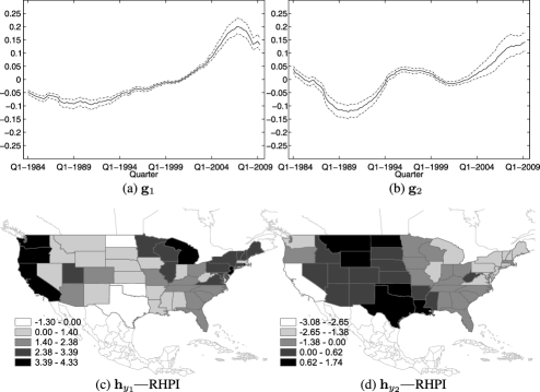
Figure 2: Subplots (a) and (b): marginal posterior medians for the estimated latent factors $g_{1}(t)$ and $g_{2}(t)$ (continuous line) and their $95\%$ credible intervals (dashed line). Subplots (c) and (d): maps of the posterior medians for the factor loadings $\mathbf{h}_{y_{1}}$ and $\mathbf{h}_{y_{2}}$ related to the real housing price index.

Figure 2(c)–(d) show the maps of the estimated first two factor loadings—that is, the first two columns of the measurement matrix $\mathbf{H}_{y}$. The maps clearly show the presence of clusters of US States. Table 2 also shows the posterior summaries of the between-location conditional correlations estimated [using equation (12)] for each column of $\mathbf{H}_{y}$. Since the $95\%$ credibility intervals do not overlap zero and all the conditional correlations seem to be statistically significant, the clusters are easily identified by looking at the spatial patterns of the factor loadings.

Table 2: Posterior summary of the between-location conditional correlations for the columns of the measurement matrix $\mathbf{H}_{y}$. In brackets we show the $2.5$ and $97.5$ percentiles used for defining the $95\%$ credible interval limits

	Factor loadings ($\mathbf{H_{y}}$)
	1	2	3	4	5	6	7
Median	0.09	0.08	0.08	0.07	0.06	0.08	0.08
$95\%$ CI	[0.05, 0.12]	[0.04, 0.12]	[0.02, 0.12]	[0.03, 0.10]	[0.03, 0.12]	[0.02, 0.12]	[0.02, 0.12]

Figure 2(c) shows [using the natural break method of ArcMap, ESRI (2009)] the weights of the first factor loading, $\mathbf{h}_{y_{1}}$. Except for Texas, Oklahoma and North Dakota, these weights are all positive, with the highest loadings observed in the Pacific and Northeast regions, which strongly influence the contiguous regions.

Figure 2(d) also shows an interesting pattern in the loadings. Southwest, Rocky Mountain States, some Plains States and Louisiana have positive loadings, while the other States have negative loadings. The States with highest loadings (Louisiana, New Mexico, Texas, Oklahoma, North Dakota and Wyoming) show a temporal pattern very similar to the second latent variables. On the other hand, the States with lowest values (California, Connecticut, Michigan, New Jersey and Rhode Island) show temporal dynamics which, at least until the end of the nineties, result in the opposite of $g_{2}(t)$. Many of these States in the last 25 years have been particular beneficiaries of new technologies. These innovations interacting with restrictions on new residential buildings have resulted in real housing prices in these regions deviating from the average across US States over a relatively prolonged period [Holly, Pesaran and Yamagata (2010)]. Also, considering the period 1984–1990, the spatial contrast highlighted in the map of Figure 2(d) clearly confirms that while West–South–Central regions (especially “oil-patch” states such as Texas and Oklahoma) experienced sharp declines, the Northeast and California housing market were booming. Note that this map provides clear evidence of the results described in Table 1 where we have found significant correlations between the States belonging to the East and West regions.

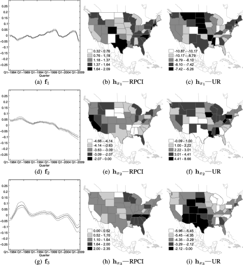
Figure 3: Subplots (a), (d) and (g): marginal posterior medians for the estimated latent factors $f_{1}(t)$, $f_{2}(t)$ and $f_{3}(t)$ (continuous line) and their $95\%$ credible intervals (dashed line). Subplots (b), (e) and (h): maps of the posterior medians for the factor loadings $\mathbf{h}_{x_{1}}$, $\mathbf{h}_{x_{2}}$ and $\mathbf{h}_{x_{3}}$ related to the real per capita personal income variable. Subplots (c), (f) and (i): maps of the posterior medians for the factor loadings $\mathbf{h}_{x_{1}}$, $\mathbf{h}_{x_{2}}$ and $\mathbf{h}_{x_{3}}$ related to the unemployment rate variable.

The MCMC estimates of the exogenous components, $f_{i}(t),i=1,\ldots,8$, summarize the dynamics of RPCI and UR variables. The first three of these latent factors, together with their $95\%$ credibility intervals, are shown in Figure 3. These components seem to have a substantial impact on RPCI and UR, although the latter shows more complex dynamics which can be fully understood by examining the behavior of all the estimated factors.

The first factor, ${f}_{1}(t)$, shows a cyclical behaviour with a slightly positive trend in the period 1986–2000. The series exhibits a trough in the period 2000–2006 followed by a sustained decrease. The 2000–2006 pattern has roots in the prior turmoil in the financial markets. In fact, the period 2000–2001 is characterized by a rapid decline of high tech industries, a collapse of the stock market and a slow level of technology investment. The relaxed monetary policy adopted by the Federal Reserve had thus lead to an increase of RPCI and a decrease of UR up to 2007.

The factor loadings related to ${f}_{1}(t)$, shown in Figure 3(b) and Figure 3(c), are all positive for RPCI and negative for UR. Figure 3(b) clearly shows groups of States with common spatial patterns. Specifically, we notice the presence of two clusters: the first involves several States from the Great Lakes, Southeast and New England, while the second is mainly characterized by Oregon and some States of the Mountain region (Arizona, Utah, Nevada and Wyoming). Also, the highest values are related to those States (Colorado, Connecticut, Georgia, Massachusetts, New Jersey, North Carolina and Texas) whose RPCI shows the same cyclical pattern of ${f}_{1}(t)$ in the period 1995–2009.

Figure 3(c), related to UR, shows quite a big cluster of States forming a ridge from Montana to Mississippi. For these States the variations of UR are less pronounced with respect to those showing the smallest loadings (e.g., Alabama, Colorado, Indiana and Virginia).

The dynamics of RPCI and UR in the first period of the series is captured by the third latent factor ${f}_{3}(t)$ shown in Figure 3(g). The figure shows that the early nineties are characterized by a trough of UR and a hill for the RPCI.

Figure 3(h) shows a huge cluster with values of the loadings in the range $1.10\mbox{--}1.64$; the highest values are observed in the Southeast region for which the oscillations of RPCI are a bit more pronounced than other States.

Figure 3(i) shows that the States for which the trough of UR is more pronounced are characterized by lowest values of the loadings. Notice that this figure also shows a reasonable correspondence with Figure 2(d).

The second factor, ${f}_{2}(t)$, shows a decreasing trend associated with negative values of $\mathbf{h}_{x_{2}}$—RPCI—and (mainly) positive values of $\mathbf{h}_{x_{2}}$—UR. The maps of the factor loading clearly provide information on those States which have experienced a positive trend for RPCI (e.g., Alabama, Arkansas, Mississippi, Nebraska, South Dakota, Tennessee and Wyoming) as well as a downward trend for UR (see, e.g., Alabama, Iowa, Louisiana, Pennsylvania and West Virginia).

The spatial structure of the factor loadings is also confirmed by the the posterior summaries of their within- and between-location conditional correlations and cross-correlations (see Table 3). The $95\%$ credibility intervals suggest that most parts of these correlations can be considered as nonzero. Also, the conditional spatial dependence of each factor loading is positive, while both the between- and the within-location conditional cross-correlations are negative.

Table 3: Posterior summary of the within- and between-location conditional correlations and cross-correlations for the first three factor loadings columns related to the unemployment rate and real per capita personal income variables. In brackets we show the $2.5$ and $97.5$ percentiles used for defining the $95\%$ credible interval limits

	Conditional correlation
	Within-location	Between-location	Between-location	Between-location	Between-location
	RPCI vs UR	RPCI	RPCI vs UR	UR vs RPCI	UR
$\mathbf{h}_{x_{1}}$	$-0.22$	0.06	$-0.04$	$-0.03$	0.05
	[$-0.44$, $-0.09$]	[0.01, 0.09]	[$-0.07$, $-0.02$]	[$-0.07$, $-0.01$]	[0.03, 0.08]
$\mathbf{h}_{x_{2}}$	$-$0.02	0.05	$-0.00$	$-0.01$	0.07
	[$-0.29$, 0.12]	[0.01, 0.10]	[$-0.06$, 0.05]	[$-0.06$, 0.06]	[0.02, 0.09]
$\mathbf{h}_{x_{3}}$	$-0.27$	0.08	$-0.02$	$-0.04$	0.07
	[$-0.38$, $-0.02$]	[0.02, 0.12]	[$-0.07$, 0.03]	[$-0.07$, $-0.01$]	[0.03, 0.10]

Model estimation: Cointegration. As noted in the introduction, there has been quite a long debate in the literature about whether there is cointegration between real housing prices and fundamentals. The idea is that in the absence of cointegration there are no fundamentals driving real housing prices and the absence of an equilibrium relationship would essentially increase the presence of bubbles [Case and Shiller (2003), Holly, Pesaran and Yamagata (2010)]. Here, we test the existence of this cointegrating relationship in a latent space, avoiding to take account of the effect of the cross-sectional dependence [see Holly, Pesaran and Yamagata (2010) for a discussion on this point]. In terms of cointegrated ranks, following Jochmann et al. (2013), our posteriors for $r_{f}$, $r_{d}$, $r_{c}$, $r_{c_{1}}$ and $r_{c_{2}}$ are obtained by considering the draws of their respective matrices (i.e., $\bolds{\Pi}_{f}$, $\bolds{\Pi}_{gd}$, $\mathbf{A}\mathbf{B}_{2}^{\prime}+\mathbf{A}_{2}\mathbf{B}_{f}^{\prime}$, $\mathbf{A}\mathbf{B}_{2}^{\prime}$ and $\mathbf{A}_{2}\mathbf{B}_{f}^{\prime}$; see Appendix A) and taking the number of singular values greater than $0.05$.

These are shown in Table 4 where we note that there is a strong support for an exogenous cointegrated rank of either 4 or 5; for $r_{d}$ there is a hint of a rank equal to 5, but small probabilities are also observed for 4 and 6. Finally, since there is evidence that $r_{c}<r_{c_{1}}+r_{c_{2}}$, we may conclude that a cointegration structure is confirmed between the endogenous and exogenous processes. Such a result thus supports the idea about the existence of a convergence to a stable equilibrium relationship and, hence, about the absence of a US housing price bubble for the period considered in the study.

Table 4: Posterior of cointegration ranks $r_{f}$, $r_{d}$, $r_{c}$, $r_{c_{1}}$ and $r_{c_{2}}$

	Estimated probabilities for effective ranks
	1	2	3	4	5	6
$r_{f}$	0.00	0.00	0.01	0.34	0.61	0.04
$r_{d}$	0.00	0.00	0.00	0.18	0.70	0.12
$r_{c}$	0.00	0.00	0.00	0.02	0.48	0.50
$r_{c_{1}}$	0.00	0.00	0.10	0.63	0.27	0.00
$r_{c_{2}}$	0.00	0.00	0.03	0.45	0.50	0.02

To provide further evidence that our approach is yielding sensible results, the use of Bayes factors using a non-SSVS prior [Sugita (2009), Kass and Raftery (1995)] confirms that, conditionally on $m=7$ and $l=8,$ results for $r_{f}$ and $r_{d}$ are similar to those presented here.

Unconditional and conditional forecasts. To test the predictive performance of the SD-SEM model, the last 10 quarters have been excluded from the estimation procedure and used only for forecast purposes. Hence, we consider the forecast for a horizon of $k=10$ periods corresponding to the quarters Q3-2009–Q4-2011. Also, predictions of RHPI are obtained by following two settings:

[(ii)]

unconditional predictions: we only use past information; hence, $X$ is not available for the forecast period;

conditional predictions: the exogenous variables $X_{1}$ and $X_{2}$ are assumed known in the period in which temporal forecasts of RHPI are required.

For each State, both unconditional and conditional forecasts (together with $95\%$ credible intervals) of the housing price index are shown in Figure 4. In general, compared with true values, good prediction results can be achieved and, as expected, the conditional (on the known values of $X$) approach exhibits more encouraging out-of-sample properties of the model, with data points being more accurately predicted.

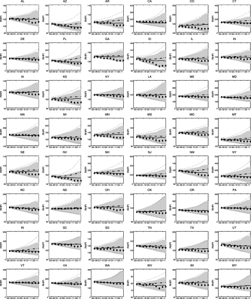
Figure 4: Unconditional forecasts (dashed line), conditional forecasts (continuous line) and true data ($\bullet$) at the 48 United States; the $95\%$ credible interval limits for the unconditional forecasts are represented by dotted lines. The $95\%$ credible interval limits for the conditional forecasts are represented by the shaded area. Each subplot also shows the initials of the State.

To provide some measures of goodness of prediction for the estimated models, Table 5 gives details on the root mean squared prediction error, $\mathrm{RMSE}=\sqrt{\operatorname{mean}\{(\tilde{Y}(\mathbf{s},t)-E[\tilde{Y}(\mathbf{s},t)_{\mathrm{rep}}])^{2}\}}$, the mean absolute error deviation, $\mathrm{MAE}=\operatorname{mean}\{|\tilde{Y}(\mathbf{s},t)-E[\tilde{Y}(\mathbf{s},t)_{\mathrm{rep}}]|\}$ [where $\tilde{Y}$ is the variable at the original scale and the mean is taken over the $({N\times k})$ observations], the coverage probabilities (CP) and the average width (AIW) of the prediction intervals. We note that in the conditional case model M₀ shows much smaller values for RMSE, MAE and AIW; on the other hand, the coverage probabilities of the 95% intervals are larger than the nominal rate. Models M₁, M₂ and M₃ provide very similar results and provide some hints on the role played by the spatially autocorrelated factor loadings and cointegrated factors. In general, model M₀ works better than M₁, M₂ and M₃ for which the average width of the prediction intervals are wider. We note that in introducing the spatial correlation the AIW reduces substantially. The same effect, albeit with different intensity, can be observed assuming cointegrated factors and this can be detected by contrasting models M₀–M₃ and M₁–M₂.

By making the series stationary through a first difference transformation, the best result of model M₄ is characterized by an RMSE of $13.575$ and a MAE of $11.372$. This result is obtained by using a GMRF prior on the regression coefficients. We also note that for this model the regressors, $X_{1}$ and $X_{2}$, are assumed as known for the forecast period. Producing unconditional predictions under model M₄, in fact, is not straightforward since it requires further adjustments for predicting the process $X$.

Table 5: Root mean squared prediction errors (RMSE), mean absolute deviations (MAE), coverage probabilities (CP) and average width (AIW) of the prediction intervals, for unconditional and conditional forecasts of RHPI. The statistics are computed for the estimated models M₀, M₁, M₂, M₃ and M₄

Model	Type of prediction	RMSE	MAE	CP 95% interval	AIW 95% interval
M0	Unconditional	$16.081$	$11.704$	0.958	$59.762$
	Conditional	$7.223$	$5.558$	0.989	$54.723$
M1	Unconditional	$17.294$	$12.950$	1.000	$140.052$
	Conditional	$9.497$	$6.614$	1.000	$138.140$
M2	Unconditional	$17.496$	$12.942$	0.989	$112.814$
	Conditional	$9.904$	$7.414$	0.998	$112.086$
M3	Unconditional	$17.150$	$12.759$	0.969	$77.042$
	Conditional	$9.331$	$6.695$	0.985	$76.445$
M4	Unconditional	–	–	–	–
	Conditional	$13.575$	$11.372$	0.920	$53.180$

Multiplier analysis. We conclude the analysis by providing some results from multiplier analysis [Lutkepohl (2005)] which is helpful to describe how the housing price index reacts over time to exogenous impulses. In this case, we can check if past values on either RPCI or UR, observed on a specific State, contain useful information to predict the variation of RHPI, in addition to the information on its past values. It can be shown (see Appendix C) that the dynamic multipliers, $\bolds{\Gamma}_{k}$, which reflect the marginal impacts of changes in the predictors $X_{1}$ and $X_{2}$, are defined as

$$\bolds{\Gamma}_{k}=\mathbf{H}_{y}\bolds{\mathfrak{J}}\bolds{\mathcal{Q}}^{k}\bolds{\mathcal{B}}\mathbf{H}_{x}^{\dagger},\qquad k=0,1,\ldots,$$

where, at the $k$th period (quarter), the $\gamma_{ij,k}$ element of the $(N\times\tilde{n}_{x})$ matrix $\bolds{\Gamma}_{k}$ represents the response of the housing price in the $i$th State to a given shock in the predictor $X_{l},l=1,2$, in State $j$, provided the effect is not contaminated by other shocks to the system. The matrices $\bolds{\mathfrak{J}}$, $\bolds{\mathcal{Q}}$ and $\bolds{\mathcal{B}}$, which contribute to determine the multipliers, are defined in Appendix C.

The impulse responses of RHPI to a $1\%$ shock in the exogenous variables, RPCI and UR, in each State, show some interesting features. However, since many possible interactions among States and variables can be envisaged, in the following we provide a summary of the results as well as a visual impression of some of the dynamic interrelationships existing in the system. Note that following Sims and Zha (1999) and Primiceri (2005), the credibility intervals of the impulse response coefficients are discussed at the 16th and 84th percentiles which, under normality, correspond to the bounds of a one-standard-deviation.

One interesting feature is that a shock in RPCI in the States belonging to New England (with the exception of Connecticut and New Jersey) does not seem to produce evident effects on RHPI. The same holds for a RPCI shock in Mideast States whose effects seem to disappear after one quarter. It thus seems that past values of RPCI, in these regions, do not help in forecasting RHPI throughout the US. At the same time, apart from New Hampshire and Maryland, the prices in New England and the Mideast do not seem to react to a RPCI shock in any other region. The housing prices in Michigan, Ohio and Illinois, belonging to the Great Lakes, also seem to behave similarly. Note that this similarity in behavior was also found by Apergis and Payne (2012) in a study on housing price convergence.

On the other hand, there is stronger evidence of the relationships between UR shock effects in the States of New England and the Mideast and RHPI responses in several States, mainly belonging to the Southeast, Plains and Southwest regions. Also, RHPI forecasts in New England and Mideast regions can be improved by exploiting UR information on other States. In any case, considering the infra-regional responses (i.e., RHPI responses of New England and Mideast States to a UR shock produced in any State belonging to the same region), we note that UR effects on the variation of RHPI disappear after one period.

Regarding the remaining BEA regions, a $1\%$ shock to either RPCI or UR seems to highlight effects on the housing prices involving quite a large network of States, particularly in the second quarter. Analyzing the impulse responses for longer periods, we note that the network of relevant relationships between the States becomes sparser. However, the most persistent effects on RHPI, which also involve a large numbers of States belonging to the Southeast, Plains, Rocky Mountain, Southwest and Far West regions, are associated to RPCI shocks in Nevada, Arizona, Georgia, Alabama and Mississippi, and to UR shocks in Illinois, South Carolina, Florida, Alabama, Iowa, South Dakota and Nebraska.

Moreover, the States whose RHPI responses are more persistent to RPCI shocks in any other State of the aforementioned regions are Florida and Nevada, while the States whose responses are more persistent to UR shocks are New Mexico, Arizona, Arkansas and Mississippi.

If we consider the sign of the impulse response coefficients, we note that, in general, a positive shock to RPCI is associated to a positive effect on RHPI. Some exceptions are observed in the first period where we can find negative coefficients. On the other hand, the scenario appears to be different for the UR case, in which we note both positive and negative effects on RHPI even for longer periods. Although we may expect that unemployment has an adverse effect on real estate prices, previous studies have nevertheless found unemployment to be positively related to housing prices. For a discussion on this point we refer the reader, for example, to Vermeulen and Van Ommeren (2009), Clayton, Miller and Peng (2010) and Moench and Ng (2011).

Finally, to provide a flavor of the type of relationship, Figure 5 shows posterior mean housing price responses (solid line) in Nevada, Oregon, Arizona, New Mexico, Utah, Idaho and California to a $1\%$ shock to RPCI in Nevada. Figure 6, instead, shows the responses in Florida, Tennessee, Alabama, Mississippi, Arkansas, West Virginia, North Carolina and Georgia to a $1\%$ shock to UR in Florida. The shaded regions indicate the credibility intervals corresponding to $68$ and $90$ percent. Overall, the plots suggest that State-level responses follow a similar pattern (consistently with the ripple effect) and, in most cases, the effects tend to decay over two years, especially for UR shocks.

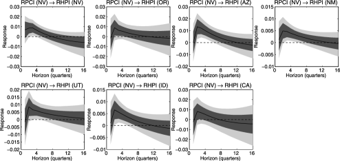
Figure 5: Posterior mean impulse responses (solid line) of RHPI to a RPCI shock in Nevada. The credibility intervals at $68\%$ and $90\%$ are represented by shaded areas. The responses are observed in Nevada (NV), Oregon (OR), Arizona (AZ), New Mexico (NM), Utah (UT), Idaho (ID) and California (CA).

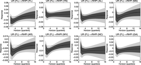
Figure 6: Posterior mean impulse responses (solid line) of RHPI to a UR shock in Florida. The credibility intervals at $68\%$ and $90\%$ are represented by shaded areas. The responses are observed in Florida (FL), Tennessee (TN), Alabama (AL), Mississippi (MS), Arkansas (AR), West Virginia (WV), North Carolina (NC) and Georgia (GA).

9 Discussion

In this paper we have discussed the modeling of spatio-temporal multivariate processes observed on a lattice by means of a Bayesian spatial dynamic structural equation model. We have used ideas from factor analysis to frame and exploit both the spatial and the temporal structure of the observed processes.

It can be shown that the SD-SEM encompasses a large class of spatial-temporal models that are commonly used and, more importantly, differs from them in two major aspects: (i) it avoids the curse of dimensionality commonly present in large spatio-temporal data and (ii) it facilitates the formation of spatial clusters which further avoids dimensionality issues.

The model has been implemented in a Bayesian setup using MCMC sampling. The MCMC chains of the parameters were monitored to detect possible problems in convergence although no such problems were found in the implementation.

The model was applied to study the impact that the real per capita personal income and the unemployment rate may have on the real housing prices in the USA using State level data. Forecasting the future economic conditions and understanding the relations between the observed variables have been two important aspects covered by our model. The spatial variation is brought into the model through the columns of the factor loading matrix and the estimated conditional correlations and cross-correlations gave significant evidence of spatial dependence associated with contiguity. The spatial patterns of the factor loadings revealed several clusters of interest showing common dynamics.

The time series dynamics have been captured by common dynamic factors. An error correction model specification, with a cointegrating relationship between the common latent factors, was found useful once we took proper account of both heterogeneity and cross-sectional dependence. Overall, results support the hypothesis that real housing prices have been rising in line with fundamentals (real incomes and unemployment rates), and there seems no evidence of housing price bubbles at the national level.

Results from multiplier analysis were also helpful to describe how the housing price index reacts over time to exogenous impulses. We have found that, consistently with the ripple effect, the RHPI responses show a similar pattern for neighboring States. The responses seem to be more persistent to UR shocks, while the effects of a RPCI shock decay more rapidly such that the system appears to approach faster to the initial equilibrium conditions.

A further important advantage of the model formulation is that it enables consideration of cases in which the temporal series of $X$ are longer than those of $Y$. As noticed in Section 7, this was particularly useful to improve the temporal predictions by conditioning on known values of the predictor providing a set of plausible scenarios for RHPI.

Of course, we acknowledge that other possibilities could be considered for modeling the spatial structure and an example is provided by Wang and Wall (2003). An alternative scheme could also lead to the specification of common factors with a spatio-temporal structure. In this case, one may follow the methodology proposed in Debarsy, Ertur and LeSage (2012) to quantify dynamic responses over time and space as well as space–time diffusion impacts.

Finally, in this paper we have focused exclusively on normally distributed data. However, nonlinear and non-Gaussian spatio-temporal models have been extensively used in various areas of science, from epidemiology to meteorology and environmental sciences, among others. In this case, assuming the measurements belong to the exponential family of distributions, a generalized spatial dynamic structural equation model represents a natural extension of the SD-SEM discussed here. This extension will be a topic for future work.

Appendix A Cointegrated latent factors and their Vector Error Correction representation

Let $\tilde{\bolds{\Phi}}(z)$ denote the characteristic polynomial associated with the vector ECM shown in (11) and let $c$ be the number of unit roots of $\operatorname{Det}[\bolds{\Phi}(z)]$. Let also that $\operatorname{rank}(\tilde{\mathbf{A}})=r$, with $r=m+l-c$. Then, we assume that the latent exogenous variables, $\mathbf{f}(t)$, are cointegrated with cointegrating rank $r_{f}$ so that $r>r_{f}$ and $r_{f}<l$.

Let $\mathbf{Q}(\sum_{i=1}^{p}\bolds{\Phi}_{i})\mathbf{P}=\mathbf{J}$ be the Jordan canonical form of $\sum_{i=1}^{p}\bolds{\Phi}_{i}$, where $\mathbf{Q}=\mathbf{P}^{-1}$ an $((m+l)\times(m+l))$ matrix, $\mathbf{J}=\operatorname{diag}(\mathbf{I}_{m-r_{d}},\bolds{\Lambda}_{r_{d}},\mathbf{I}_{l-r_{f}},\bolds{\Lambda}_{r_{f}})$ and $r_{d}\equiv r-r_{f}$ [Ahn and Reinsel (1990) and Cho (2010)]. Because of the exogeneity of $\mathbf{f}(t)$, the matrices $\tilde{\mathbf{A}}$ and $\tilde{\bolds{\Phi}}_{i}$ are upper block triangular matrices, that is,

$$\tilde{\mathbf{A}}=\left[\matrix{\tilde{\mathbf{A}}_{1}&\tilde{\mathbf{A}}_{12}\vspace*{2pt}\cr\mathbf{0}&\tilde{\mathbf{A}}_{2}}\right]\quad\mbox{and}\quad\tilde{\bolds{\Phi}}_{i}=\left[\matrix{\tilde{\bolds{\Phi}}_{1i}&\tilde{\bolds{\Phi}}_{12i}\vspace*{2pt}\cr\mathbf{0}&\tilde{\bolds{\Phi}}_{2i}}\right].$$

Then, consider the following matrix partition:

$$\mathbf{P}=\left[\matrix{\mathbf{P}_{1}&\mathbf{P}_{12}\vspace*{2pt}\cr\mathbf{0}&\mathbf{P}_{2}}\right],\qquad\mathbf{Q}=\mathbf{P}^{-1}=\left[\matrix{\mathbf{P}_{1}^{-1}&-\mathbf{P}_{1}^{-1}\mathbf{P}_{12}\mathbf{P}_{2}^{-1}\vspace*{2pt}\cr\mathbf{0}&\mathbf{P}_{2}^{-1}}\right]=\left[\matrix{\mathbf{Q}_{1}&\mathbf{Q}_{12}\vspace*{2pt}\cr\mathbf{0}&\mathbf{Q}_{2}}\right],$$

with $\mathbf{Q}_{1}^{\prime}=[{\mathbf{Q}_{1}^{(1)}\enskip\mathbf{Q}_{1}^{(2)}}]$, $\mathbf{P}_{1}=[{\mathbf{P}_{1}^{(1)}\enskip\mathbf{P}_{1}^{(2)}}]$, $\mathbf{Q}_{12}^{\prime}=[{\mathbf{Q}_{12}^{(1)}\enskip\mathbf{Q}_{12}^{(2)}}]$, $\mathbf{P}_{12}=[{\mathbf{P}_{12}^{(1)}\enskip\mathbf{P}_{12}^{(2)}}]$, $\mathbf{Q}_{2}^{\prime}=[{\mathbf{Q}_{2}^{(1)}\enskip\mathbf{Q}_{2}^{(2)}}]$ and $\mathbf{P}_{2}=[{\mathbf{P}_{2}^{(1)}\enskip\mathbf{P}_{2}^{(2)}}]$.

Note that $\mathbf{Q}_{1}^{(1)}$, $\mathbf{P}_{1}^{(1)}$ are $(m\times(m-r_{d}))$, $\mathbf{Q}_{1}^{(2)}$, $\mathbf{P}_{1}^{(2)}$ are $(m\times r_{d})$, $\mathbf{Q}_{2}^{(1)}$, $\mathbf{P}_{2}^{(1)}$ are $(l\times(l-r_{f}))$, $\mathbf{Q}_{2}^{(2)}$, $\mathbf{P}_{2}^{(2)}$ are $(l\times r_{f})$, $\mathbf{Q}_{12}^{(1)}$ is $(l\times(m-r_{d}))$, $\mathbf{P}_{12}^{(1)}$ is $(m\times(l-r_{f}))$, $\mathbf{Q}_{12}^{(2)}$ is $(l\times r_{d})$ and $\mathbf{P}_{12}^{(2)}$ is $(m\times r_{f}).$ Then, we may write

$$\tilde{\mathbf{A}} = -\mathbf{P}(\mathbf{I}-\mathbf{J})\mathbf{Q}=-\left[\matrix{\mathbf{P}_{1}^{(2)}&\mathbf{P}_{12}^{(2)}\vspace*{2pt}\cr\mathbf{0}&\mathbf{P}_{2}^{(2)}}\right]\left[\matrix{\mathbf{I}-\bolds{\Lambda}_{r_{d}}&\mathbf{0}\vspace*{2pt}\cr\mathbf{0}&\mathbf{I}-\bolds{\Lambda}_{r_{f}}}\right]\left[\matrix{\mathbf{Q}_{1}^{(2)^{\prime}}&\mathbf{Q}_{12}^{(2)^{\prime}}\vspace*{2pt}\cr\mathbf{0}&\mathbf{Q}_{2}^{(2)^{\prime}}}\right]$$

$$= -\left[\matrix{\mathbf{P}_{1}^{(2)}(\mathbf{I}-\bolds{\Lambda}_{r_{d}})\mathbf{Q}_{1}^{(2)^{\prime}}&\mathbf{P}_{1}^{(2)}(\mathbf{I}-\bolds{\Lambda}_{r_{d}})\mathbf{Q}_{1}^{(2)^{\prime}}\mathbf{P}_{12}\mathbf{Q}_{2}+\mathbf{P}_{12}^{(2)}(\mathbf{I}-\bolds{\Lambda}_{r_{f}})\mathbf{Q}_{2}^{(2)^{\prime}}\vspace*{2pt}\cr\mathbf{0}&\mathbf{P}_{2}^{(2)}(\mathbf{I}-\bolds{\Lambda}_{r_{f}})\mathbf{Q}_{2}^{(2)^{\prime}}}\right],$$

and equation (11) can thus be rewritten as

$$\Delta\mathbf{g}(t) = \mathbf{A}\mathbf{B}^{\prime}\mathbf{d}(t-1)+\mathbf{A}_{2}\mathbf{B}_{f}^{\prime}\mathbf{f}(t-1)+\sum_{i=1}^{p-1}\mathbf{K}_{i}\Delta\mathbf{d}(t-i)+\bolds{\xi}(t),$$ (13)

$$\Delta\mathbf{f}(t) = \mathbf{A}_{f}\mathbf{B}_{f}^{\prime}\mathbf{f}(t-1)+\sum_{i=1}^{p-1}\tilde{\bolds{\Phi}}_{2i}\Delta\mathbf{f}(t-j)+\bolds{\eta}(t),$$ (14)

where $\mathbf{A}=-\mathbf{P}_{1}^{(2)}(\mathbf{I}-\bolds{\Lambda}_{r_{d}})$, $\mathbf{B}=[{\mathbf{I}\enskip-\mathbf{P}_{12}\mathbf{Q}_{2}}]^{\prime}\mathbf{Q}_{1}^{(2)}$, $\mathbf{A}_{f}=-\mathbf{P}_{2}^{(2)}(\mathbf{I}-\bolds{\Lambda}_{r_{f}})$, $\mathbf{A}_{2}=-\mathbf{P}_{12}^{(2)}(\mathbf{I}-\bolds{\Lambda}_{r_{f}})$, $\mathbf{B}_{f}=\mathbf{Q}_{2}^{(2)}$ and $\mathbf{K}_{i}=[{\tilde{\bolds{\Phi}}_{1i}\enskip\tilde{\bolds{\Phi}}_{12i}}]$. Note that if $\mathbf{P}_{12}$ and $\mathbf{P}_{12}^{(2)}$ are $\mathbf{0}$, then a separated cointegrated structure exists for $\mathbf{g}(t)$ and $\mathbf{f}(t)$.

Let $\mathbf{B}=[{\mathbf{B}_{1}^{\prime}\enskip\mathbf{B}_{2}^{\prime}}]^{\prime}$ where $\mathbf{B}_{1}=\mathbf{Q}_{1}^{(2)}$ and $\mathbf{B}_{2}=-\mathbf{Q}_{2}^{\prime}\mathbf{P}_{12}^{\prime}\mathbf{Q}_{1}^{(2)}$, then $\tilde{\mathbf{A}}$ can be rewritten as

$$\tilde{\mathbf{A}}=-\left[\matrix{\mathbf{A}\mathbf{B}_{1}^{\prime}&\mathbf{A}\mathbf{B}_{2}^{\prime}+\mathbf{A}_{2}\mathbf{B}_{f}^{\prime}\vspace*{2pt}\cr\mathbf{0}&\mathbf{A}_{f}\mathbf{B}_{f}^{\prime}}\right].$$

Also, let $r_{f}=\operatorname{rank}(\mathbf{A}_{f}\mathbf{B}_{f}^{\prime})$, $r_{d}=\operatorname{rank}(\mathbf{A}\mathbf{B}^{\prime})$, $r_{c}=\operatorname{rank}(\mathbf{A}\mathbf{B}_{2}^{\prime}+\mathbf{A}_{2}\mathbf{B}_{f}^{\prime})$, $r_{c_{1}}=\operatorname{rank}(\mathbf{A}\mathbf{B}_{2}^{\prime})$ and $r_{c_{2}}=\operatorname{rank}(\mathbf{A}_{2}\mathbf{B}_{f}^{\prime}).$ Then, it follows that if $\operatorname{rank}(\mathbf{A}\mathbf{B}_{2}^{\prime}+\mathbf{A}_{2}\mathbf{B}_{f}^{\prime})=0$, no cointegration structure exists between the endogenous and exogenous processes $\mathbf{g}(t)$ and $\mathbf{f}(t)$.

Appendix B The SSVS prior for the vector ECM

Since $\bolds{\Pi}_{gd}=\mathbf{A}\mathbf{B}^{\prime}$, $\bolds{\Pi}_{gf}=\mathbf{A}_{2}\mathbf{B}_{f}^{\prime}$ and $\bolds{\Pi}_{f}=\mathbf{A}_{f}\mathbf{B}_{f}^{\prime}$ are not unique, in this paper we follow the approach proposed by Jochmann et al. (2013) and Koop, León-González and Strachan (2010) to elicit the SSVS priors on the cointegration space. A summary of this approach is provided below.

Specifically, a nonidentified $r^{*}_{d}\times r^{*}_{d}$ symmetric positive definite matrix $\mathbf{E}$ is introduced with the property, $\bolds{\Pi}_{gd}=\mathbf{A}\mathbf{E}\mathbf{E}^{-1}\mathbf{B}^{\prime}\equiv\bar{\mathbf{A}}\bar{\mathbf{B}}^{\prime}$, where $\bar{\mathbf{A}}=\mathbf{A}\mathbf{E}$ and $\bar{\mathbf{B}}=\mathbf{B}\mathbf{E}^{-1}$. The introduction of the nonidentified matrix $\mathbf{E}$ facilitates posterior computation because the posterior conditional distributions of $\bar{\mathbf{A}}$ and $\bar{\mathbf{B}}$ in the MCMC algorithm are Gaussian [Koop, León-González and Strachan (2010)]. The same holds analogously for $\bolds{\Pi}_{gf}$ and $\bolds{\Pi}_{f}$.

Let $\bar{\mathbf{a}}=\operatorname{vec}(\bar{\mathbf{A}}^{\prime})$ and $\bolds{\rho}=(\rho_{1},\ldots,\rho_{\tilde{m}})$ a parameter vector, where $\tilde{m}=mr^{*}_{d}$. Then, we assume that $\bar{\mathbf{a}}|\bolds{\rho}\sim N(\mathbf{0},\mathbf{V}_{0})$, where $\mathbf{V}_{0}=\operatorname{diag}(v_{1}^{2},\ldots,v_{\tilde{m}}^{2})$, $v_{i}^{2}=(1-\rho_{i})v_{0i}^{2}+\rho_{i}v_{1i}^{2}$ and $\rho_{i}$, the $i$th element of $\bolds{\rho}$, has a Bernoulli distribution with parameter $p_{a}$, that is, $\rho_{i}\sim\operatorname{Be}(p_{a})$. In this paper, we set $p_{a}=0.5$, $v_{0i}^{2}=0.1\hat{\sigma}^{2}(\bar{a}_{i})$, $v_{1i}^{2}=10\hat{\sigma}^{2}(\bar{a}_{i})$, where $\hat{\sigma}^{2}(\bar{a}_{i})$ is an estimate of the variance of the $i$th element of $\bar{\mathbf{a}}$ obtained from a preliminary MCMC run with a noninformative prior.

With appropriate notation, the same assumptions hold for $\bar{\mathbf{a}}_{f}=\operatorname{vec}(\bar{\mathbf{A}}_{f})$, with $\bar{\mathbf{A}}_{f}=\mathbf{A}_{f}\mathbf{E}_{f}$, and $\bar{\mathbf{a}}_{2}=\operatorname{vec}(\bar{\mathbf{A}}_{2})$, with $\bar{\mathbf{A}}_{2}=\mathbf{A}_{2}\mathbf{E}_{f}$.

The prior for the cointegrated space is defined through $\bar{\mathbf{b}}\sim N(\mathbf{0},\mathbf{I})$ and $\bar{\mathbf{b}}_{f}\sim N(\mathbf{0},\mathbf{I})$, where $\bar{\mathbf{b}}=\operatorname{vec}(\bar{\mathbf{B}})$, $\bar{\mathbf{b}}_{f}=\operatorname{vec}(\bar{\mathbf{B}}_{f})$ and $\bar{\mathbf{B}}_{f}=\mathbf{B}\mathbf{E}_{f}^{-1}$. The SSVS prior for $\mathbf{k}=\operatorname{vec}([\mathbf{K}_{1},\ldots,\mathbf{K}_{p^{*}-1}]^{\prime})$ is given by $\mathbf{k}|\bolds{\delta}\sim N(\mathbf{0},\mathbf{D})$, where $\mathbf{D}=\operatorname{diag}(\tau_{1}^{2},\ldots,\tau_{(m+l)(p^{*}-1)}^{2})$, $\tau_{i}^{2}=(1-\delta_{i})\tau_{0i}^{2}+\delta_{i}\tau_{1i}^{2}$ and $\bolds{\delta}$ is an unknown vector with typical element $\delta_{i}\sim\operatorname{Be}(p_{\tau})$. Here, we set $p_{\tau}=0.5$, $\tau_{0i}^{2}=0.1\hat{\sigma}^{2}(k_{i})$, $\tau_{1i}^{2}=10\hat{\sigma}^{2}(k_{i})$, and $\hat{\sigma}^{2}(k_{i})$ is an estimate of the variance of the $i$th element of $\mathbf{k}$ obtained from a preliminary MCMC run using a noninformative prior. Analogously, we define $\bolds{\phi}=\operatorname{vec}([\tilde{\bolds{\Phi}}_{21},\ldots,\tilde{\bolds{\Phi}}_{2p^{*}-1}]^{\prime})$ and assume that $\bolds{\phi}|\bolds{\delta}_{\phi}\sim N(\mathbf{0},\mathbf{D}_{\phi})$, where $\mathbf{D}_{\phi}=\operatorname{diag}(\kappa_{\phi 1}^{2},\ldots,\kappa_{\phi m^{2}(p^{*}-1)}^{2})$, $\kappa_{\phi i}^{2}=(1-\delta_{\phi i})\kappa_{\phi 0i}^{2}+\delta_{\phi i}\kappa_{\phi 1i}^{2}$ and $\bolds{\delta}_{\phi}$ is an unknown vector with element $\delta_{\phi i}\sim\operatorname{Be}(p_{\phi})$. Here we set $p_{\phi}=0.5$, $\kappa_{\phi 0i}^{2}=0.1\hat{\sigma}^{2}(\bar{\phi}_{i})$, $\kappa_{\phi 1i}^{2}=10\hat{\sigma}^{2}(\bar{\phi}_{i})$, and $\hat{\sigma}^{2}(\bar{\phi}_{i})$ is an estimate of the variance of the $i$th element of $\bar{\bolds{\phi}}$ obtained from a preliminary MCMC run using a noninformative prior.

Appendix C Multiplier analysis

If the model contains integrated variables and the generation mechanism is started at time $t=0$, it readily follows that [Lütkepohl (2005), page 402–407]

$$\mathbf{g}(t)=\bolds{\mathfrak{J}}\bolds{\mathcal{Q}}^{t}\mathbf{g}(0)+\sum_{i=0}^{t-1}\bolds{\mathfrak{J}}\bolds{\mathcal{Q}}^{i}\bolds{\mathcal{B}}\mathbf{f}(t-i)+\sum_{i=0}^{t-1}\bolds{\mathfrak{J}}\bolds{\mathcal{Q}}^{i}\bolds{\mathfrak{J}}^{\prime}\bolds{\xi}(t-i),$$ (15)

where $\bolds{\mathfrak{J}}$, $\bolds{\mathcal{B}}$ and $\bolds{\mathcal{Q}}$ are $(m\times(mp+ls))$, $((mp+ls)\times l)$ and $((mp+ls)\times(mp+ls))$ matrices such that

$$\bolds{\mathfrak{J}} = \left[\matrix{\mathbf{I}&\mathbf{0}&\cdots&\mathbf{0}}\right],$$

$$\bolds{\mathcal{B}} = \left[\matrix{\mathbf{0}\vspace*{2pt}\cr\mathbf{0}\vspace*{2pt}\cr\vdots\vspace*{2pt}\cr\mathbf{0}\vspace*{2pt}\cr\mathbf{I}_{l}\vspace*{2pt}\cr\mathbf{0}\vspace*{2pt}\cr\vdots\vspace*{2pt}\cr\mathbf{0}}\right],\qquad\bolds{\mathcal{Q}}=\left[\matrix{\mathbf{C}_{1}&\mathbf{C}_{2}&\cdots&\mathbf{C}_{p}&\mathbf{D}_{1}&\cdots&\mathbf{D}_{2}&\mathbf{D}_{s}\vspace*{2pt}\cr\mathbf{I}_{m}&\mathbf{0}&\cdots&\mathbf{0}&\mathbf{0}&\cdots&\mathbf{0}&\mathbf{0}\vspace*{2pt}\cr\vdots&\vdots&\vdots&\vdots&\vdots&\vdots&\vdots&\vdots\vspace*{2pt}\cr\mathbf{0}&\cdots&\mathbf{I}_{m}&\mathbf{0}&\mathbf{0}&\cdots&\mathbf{0}&\mathbf{0}\vspace*{2pt}\cr\mathbf{0}&\cdots&\mathbf{0}&\mathbf{0}&\mathbf{0}&\mathbf{0}&\cdots&\mathbf{0}\vspace*{2pt}\cr\mathbf{0}&\cdots&\mathbf{0}&\mathbf{0}&\mathbf{I}_{l}&\mathbf{0}&\cdots&\mathbf{0}\vspace*{2pt}\cr\vdots&\vdots&\vdots&\vdots&\vdots&\ddots&\vdots&\vdots\vspace*{2pt}\cr\mathbf{0}&\cdots&\mathbf{0}&\mathbf{0}&\mathbf{0}&\cdots&\mathbf{I}_{l}&\mathbf{0}}\right].$$

Then, assuming without loss of generality $\mathbf{m}_{x}(t)=\mathbf{0}$ and $\mathbf{m}_{y}(t)=\mathbf{0}$, it follows from the measurement equation (1) that by denoting with $\mathbf{H}_{x}^{\dagger}$ the pseudo-inverse of $\mathbf{H}_{x}$, that is, $\mathbf{H}_{x}^{\dagger}=(\mathbf{H}_{x}^{\prime}\mathbf{H}_{x})^{-1}\mathbf{H}_{x}^{\prime}$, for $m<\tilde{n}_{x}$ and $\mathbf{H}_{x}^{\prime}\mathbf{H}_{x}$ invertible, the least-square estimator of $\mathbf{f}(t)$ is $\hat{\mathbf{f}}(t)=\mathbf{H}_{x}^{\dagger}\mathbf{X}(t).$

Hence, from equations (2) and (15), it follows that the marginal impact of changes of the predictor $\mathbf{X}(t)$ on the dependent variable $\mathbf{Y}(t)$ can be investigated through the coefficient matrices

$$\bolds{\Gamma}_{k}=\mathbf{H}_{y}\bolds{\mathfrak{J}}\bolds{\mathcal{Q}}^{k}\bolds{\mathcal{B}}\mathbf{H}_{x}^{\dagger},\qquad k=0,1,\ldots$$

References

- Ahn and Reinsel (1990) {barticle}[mr] \bauthor\bsnmAhn, \bfnmSung K.\binitsS. K. and \bauthor\bsnmReinsel, \bfnmGregory C.\binitsG. C. (\byear1990). \btitleEstimation for partially nonstationary multivariate autoregressive models. \bjournalJ. Amer. Statist. Assoc. \bvolume85 \bpages813–823. \bidissn=0162-1459, mr=1138362 \bptokimsref \endbibitem
- Anselin (1988) {bbook}[auto:STB—2013/02/26—09:05:15] \bauthor\bsnmAnselin, \bfnmL.\binitsL. (\byear1988). \btitleSpatial Econometrics: Models and Applications. \bpublisherKluwer Academic, \blocationDordrecht, The Netherlands. \bptokimsref \endbibitem
- Apergis and Payne (2012) {barticle}[auto:STB—2013/02/26—09:05:15] \bauthor\bsnmApergis, \bfnmN.\binitsN. and \bauthor\bsnmPayne, \bfnmJ. E.\binitsJ. E. (\byear2012). \btitleConvergence in U.S. housing prices by state: Evidence from the club convergence and clustering procedure. \bjournalLetters in Spatial and Resource Sciences \bvolume5 \bpages103–111. \bptokimsref \endbibitem
- Banerjee, Carlin and Gelfand (2004) {bbook}[auto:STB—2013/02/26—09:05:15] \bauthor\bsnmBanerjee, \bfnmS.\binitsS., \bauthor\bsnmCarlin, \bfnmB. P.\binitsB. P. and \bauthor\bsnmGelfand, \bfnmA. E.\binitsA. E. (\byear2004). \btitleHierarchical Modeling and Analysis for Spatial Data. \bpublisherChapman & Hall/CRC, \blocationBoca Raton, FL. \bptokimsref \endbibitem
- Box, Jenkins and Reinsel (1994) {bbook}[mr] \bauthor\bsnmBox, \bfnmGeorge E. P.\binitsG. E. P., \bauthor\bsnmJenkins, \bfnmGwilym M.\binitsG. M. and \bauthor\bsnmReinsel, \bfnmGregory C.\binitsG. C. (\byear1994). \btitleTime Series Analysis: Forecasting and Control, \bedition3rd ed. \bpublisherPrentice Hall Inc., \blocationEnglewood Cliffs, NJ. \bidmr=1312604 \bptokimsref \endbibitem
- Brown, Vannucci and Fearn (1998) {barticle}[mr] \bauthor\bsnmBrown, \bfnmP. J.\binitsP. J., \bauthor\bsnmVannucci, \bfnmM.\binitsM. and \bauthor\bsnmFearn, \bfnmT.\binitsT. (\byear1998). \btitleMultivariate Bayesian variable selection and prediction. \bjournalJ. R. Stat. Soc. Ser. B Stat. Methodol. \bvolume60 \bpages627–641. \biddoi=10.1111/1467-9868.00144, issn=1369-7412, mr=1626005 \bptokimsref \endbibitem
- Cameron, Muellbauer and Murphy (2006) {bbook}[auto:STB—2013/02/26—09:05:15] \bauthor\bsnmCameron, \bfnmG.\binitsG., \bauthor\bsnmMuellbauer, \bfnmJ.\binitsJ. and \bauthor\bsnmMurphy, \bfnmA.\binitsA. (\byear2006). \btitleWas There a British House Price Bubble? Evidence from a Regional Panel. Mimeo. \bpublisherOxford Univ. Press, \blocationLondon. \bptokimsref \endbibitem
- Capozza et al. (2002) {bmisc}[auto:STB—2013/02/26—09:05:15] \bauthor\bsnmCapozza, \bfnmD. R.\binitsD. R., \bauthor\bsnmHendershott, \bfnmP. H.\binitsP. H., \bauthor\bsnmMack, \bfnmC.\binitsC. and \bauthor\bsnmMayer, \bfnmC. J.\binitsC. J. (\byear2002). \bhowpublishedDeterminants of real house price dynamics. NBER Working Paper 9262. \bptokimsref \endbibitem
- Carter and Kohn (1994) {barticle}[mr] \bauthor\bsnmCarter, \bfnmC. K.\binitsC. K. and \bauthor\bsnmKohn, \bfnmR.\binitsR. (\byear1994). \btitleOn Gibbs sampling for state space models. \bjournalBiometrika \bvolume81 \bpages541–553. \biddoi=10.1093/biomet/81.3.541, issn=0006-3444, mr=1311096 \bptokimsref \endbibitem
- Case and Shiller (2003) {barticle}[auto:STB—2013/02/26—09:05:15] \bauthor\bsnmCase, \bfnmK. E.\binitsK. E. and \bauthor\bsnmShiller, \bfnmR. J.\binitsR. J. (\byear2003). \btitleIs there a bubble in the housing market? \bjournalBrookings Papers on Economic Activity \bvolume2 \bpages299–362. \bptokimsref \endbibitem
- Cho (2010) {bmisc}[auto:STB—2013/02/26—09:05:15] \bauthor\bsnmCho, \bfnmS.\binitsS. (\byear2010). \bhowpublishedInference of cointegrated model with exogenous variables. SIRFE Working Paper 10–A04. \bptokimsref \endbibitem
- Clayton, Miller and Peng (2010) {barticle}[auto:STB—2013/02/26—09:05:15] \bauthor\bsnmClayton, \bfnmJ.\binitsJ., \bauthor\bsnmMiller, \bfnmN.\binitsN. and \bauthor\bsnmPeng, \bfnmL.\binitsL. (\byear2010). \btitlePrice-volume correlation in the housing market: Causality and co-movements. \bjournalJournal of Real Estate Finance and Economics \bvolume40 \bpages14–40. \bptokimsref \endbibitem
- Cressie (1993) {bbook}[mr] \bauthor\bsnmCressie, \bfnmNoel A. C.\binitsN. A. C. (\byear1993). \btitleStatistics for Spatial Data. \bseriesWiley Series in Probability and Mathematical Statistics: Applied Probability and Statistics. \bpublisherWiley, \blocationNew York. \bidmr=1239641 \bptokimsref \endbibitem
- Dawid (1981) {barticle}[mr] \bauthor\bsnmDawid, \bfnmA. P.\binitsA. P. (\byear1981). \btitleSome matrix-variate distribution theory: Notational considerations and a Bayesian application. \bjournalBiometrika \bvolume68 \bpages265–274. \biddoi=10.1093/biomet/68.1.265, issn=0006-3444, mr=0614963 \bptokimsref \endbibitem
- Debarsy, Ertur and LeSage (2012) {barticle}[mr] \bauthor\bsnmDebarsy, \bfnmNicolas\binitsN., \bauthor\bsnmErtur, \bfnmCem\binitsC. and \bauthor\bsnmLeSage, \bfnmJames P.\binitsJ. P. (\byear2012). \btitleInterpreting dynamic space–time panel data models. \bjournalStat. Methodol. \bvolume9 \bpages158–171. \biddoi=10.1016/j.stamet.2011.02.002, issn=1572-3127, mr=2863605 \bptokimsref \endbibitem
- Di Giacinto et al. (2005) {barticle}[mr] \bauthor\bsnmDi Giacinto, \bfnmValter\binitsV., \bauthor\bsnmDryden, \bfnmIan\binitsI., \bauthor\bsnmIppoliti, \bfnmLuigi\binitsL. and \bauthor\bsnmRomagnoli, \bfnmLuca\binitsL. (\byear2005). \btitleLinear smoothing of noisy spatial temporal series. \bjournalJ. Math. Stat. \bvolume1 \bpages299–311. \bidissn=1549-3644, mr=2400983 \bptokimsref \endbibitem
- Durbin and Koopman (2001) {bbook}[mr] \bauthor\bsnmDurbin, \bfnmJ.\binitsJ. and \bauthor\bsnmKoopman, \bfnmS. J.\binitsS. J. (\byear2001). \btitleTime Series Analysis by State Space Methods. \bseriesOxford Statistical Science Series \bvolume24. \bpublisherOxford Univ. Press, \blocationOxford. \bidmr=1856951 \bptokimsref \endbibitem
- Elhorst (2001) {barticle}[auto:STB—2013/02/26—09:05:15] \bauthor\bsnmElhorst, \bfnmJ. P.\binitsJ. P. (\byear2001). \btitleDynamic models in space and time. \bjournalGeographical Analysis \bvolume33 \bpages119–140. \bptokimsref \endbibitem
- Engle, Hendry and Richard (1983) {barticle}[mr] \bauthor\bsnmEngle, \bfnmRobert F.\binitsR. F., \bauthor\bsnmHendry, \bfnmDavid F.\binitsD. F. and \bauthor\bsnmRichard, \bfnmJean-François\binitsJ.-F. (\byear1983). \btitleExogeneity. \bjournalEconometrica \bvolume51 \bpages277–304. \biddoi=10.2307/1911990, issn=0012-9682, mr=0688727 \bptokimsref \endbibitem
- ESRI (2009) {bmisc}[auto:STB—2013/02/26—09:05:15] \borganizationESRI. (\byear2009). \bhowpublishedArcMap 9.2. Environmental Systems Resource Institute, Redlands, California. \bptokimsref \endbibitem
- Frühwirth-Schnatter (1994) {barticle}[mr] \bauthor\bsnmFrühwirth-Schnatter, \bfnmSylvia\binitsS. (\byear1994). \btitleData augmentation and dynamic linear models. \bjournalJ. Time Series Anal. \bvolume15 \bpages183–202. \biddoi=10.1111/j.1467-9892.1994.tb00184.x, issn=0143-9782, mr=1263889 \bptokimsref \endbibitem
- Gallin (2008) {barticle}[auto:STB—2013/02/26—09:05:15] \bauthor\bsnmGallin, \bfnmJ.\binitsJ. (\byear2008). \btitleThe long run relationship between housing prices and income: Evidence from local housing markets. \bjournalReal Estate Economics \bvolume36 \bpages635–658. \bptokimsref \endbibitem
- Gelfand and Ghosh (1998) {barticle}[mr] \bauthor\bsnmGelfand, \bfnmAlan E.\binitsA. E. and \bauthor\bsnmGhosh, \bfnmSujit K.\binitsS. K. (\byear1998). \btitleModel choice: A minimum posterior predictive loss approach. \bjournalBiometrika \bvolume85 \bpages1–11. \biddoi=10.1093/biomet/85.1.1, issn=0006-3444, mr=1627258 \bptokimsref \endbibitem
- Gelman (1996) {bmisc}[auto:STB—2013/02/26—09:05:15] \bauthor\bsnmGelman, \bfnmA.\binitsA. (\byear1996). \bhowpublishedInference and Monitoring Convergence. In Introducing Markov Chain Monte Carlo. \bptokimsref \endbibitem
- George, Sun and Ni (2008) {barticle}[mr] \bauthor\bsnmGeorge, \bfnmEdward I.\binitsE. I., \bauthor\bsnmSun, \bfnmDongchu\binitsD. and \bauthor\bsnmNi, \bfnmShawn\binitsS. (\byear2008). \btitleBayesian stochastic search for VAR model restrictions. \bjournalJ. Econometrics \bvolume142 \bpages553–580. \biddoi=10.1016/j.jeconom.2007.08.017, issn=0304-4076, mr=2408749 \bptokimsref \endbibitem
- Geweke (1992) {bincollection}[mr] \bauthor\bsnmGeweke, \bfnmJohn\binitsJ. (\byear1992). \btitleEvaluating the accuracy of sampling-based approaches to the calculation of posterior moments. In \bbooktitleBayesian Statistics, 4 (PeñíScola, 1991) (\beditor\binitsJ.\bfnmJ. \bsnmBernardo, \beditor\binitsJ.\bfnmJ. \bsnmBerger, \beditor\binitsA.\bfnmA. \bsnmDawid and \beditor\binitsA.\bfnmA. \bsnmSmith, eds.) \bpages169–193. \bpublisherOxford Univ. Press, \blocationNew York. \bidmr=1380276 \bptokimsref \endbibitem
- Gilks, Richardson and Spiegelhalter (1996) {bbook}[mr] \beditor\bsnmGilks, \bfnmW. R.\binitsW. R., \beditor\bsnmRichardson, \bfnmS.\binitsS. and \beditor\bsnmSpiegelhalter, \bfnmD. J.\binitsD. J., eds. (\byear1996). \btitleMarkov Chain Monte Carlo in Practice. \bseriesInterdisciplinary Statistics. \bpublisherChapman & Hall, \blocationLondon. \bidmr=1397966 \bptokimsref \endbibitem
- Giussani and Hadjimatheou (1991) {barticle}[auto:STB—2013/02/26—09:05:15] \bauthor\bsnmGiussani, \bfnmB.\binitsB. and \bauthor\bsnmHadjimatheou, \bfnmG.\binitsG. (\byear1991). \btitleModeling regional housing prices in the United Kingdom. \bjournalPapers In Regional Science \bvolume70 \bpages201–219. \bptokimsref \endbibitem
- Gourieroux and Monfort (1997) {bbook}[auto:STB—2013/02/26—09:05:15] \bauthor\bsnmGourieroux, \bfnmC. S.\binitsC. S. and \bauthor\bsnmMonfort, \bfnmA.\binitsA. (\byear1997). \btitleTime Series and Dynamic Models. \bpublisherCambridge Univ. Press, \blocationCambridge. \bptokimsref \endbibitem
- Holly, Pesaran and Yamagata (2010) {barticle}[mr] \bauthor\bsnmHolly, \bfnmSean\binitsS., \bauthor\bsnmPesaran, \bfnmM. Hashem\binitsM. H. and \bauthor\bsnmYamagata, \bfnmTakashi\binitsT. (\byear2010). \btitleA spatio-temporal model of house prices in the USA. \bjournalJ. Econometrics \bvolume158 \bpages160–173. \biddoi=10.1016/j.jeconom.2010.03.040, issn=0304-4076, mr=2671272 \bptokimsref \endbibitem
- Ippoliti, Valentini and Gamerman (2012) {barticle}[mr] \bauthor\bsnmIppoliti, \bfnmL.\binitsL., \bauthor\bsnmValentini, \bfnmP.\binitsP. and \bauthor\bsnmGamerman, \bfnmD.\binitsD. (\byear2012). \btitleSpace-time modelling of coupled spatio-temporal environmental variables. \bjournalJ. R. Stat. Soc. Ser. C. Appl. Stat. \bvolume61 \bpages175–200. \biddoi=10.1111/j.1467-9876.2011.01011.x, issn=0035-9254, mr=2905058 \bptokimsref \endbibitem
- Jochmann et al. (2013) {barticle}[auto:STB—2013/02/26—09:05:15] \bauthor\bsnmJochmann, \bfnmM.\binitsM., \bauthor\bsnmKoop, \bfnmG.\binitsG., \bauthor\bsnmLeon-Gonzalez, \bfnmR.\binitsR. and \bauthor\bsnmStrachan, \bfnmR.\binitsR. (\byear2013). \btitleStochastic search variable selection in vector error correction models with an application to a model of the UK macroeconomy. \bjournalJ. Appl. Econometrics \bvolume28 \bpages62–81. \biddoi=10.1002/jae.1238 \bptokimsref \endbibitem
- Johansen (1988) {barticle}[mr] \bauthor\bsnmJohansen, \bfnmSøren\binitsS. (\byear1988). \btitleStatistical analysis of cointegration vectors. \bjournalJ. Econom. Dynam. Control \bvolume12 \bpages231–254. \biddoi=10.1016/0165-1889(88)90041-3, issn=0165-1889, mr=0986516 \bptokimsref \endbibitem
- Jones et al. (2006) {barticle}[mr] \bauthor\bsnmJones, \bfnmGalin L.\binitsG. L., \bauthor\bsnmHaran, \bfnmMurali\binitsM., \bauthor\bsnmCaffo, \bfnmBrian S.\binitsB. S. and \bauthor\bsnmNeath, \bfnmRonald\binitsR. (\byear2006). \btitleFixed-width output analysis for Markov chain Monte Carlo. \bjournalJ. Amer. Statist. Assoc. \bvolume101 \bpages1537–1547. \biddoi=10.1198/016214506000000492, issn=0162-1459, mr=2279478 \bptokimsref \endbibitem
- Kass and Raftery (1995) {barticle}[auto:STB—2013/02/26—09:05:15] \bauthor\bsnmKass, \bfnmR. E.\binitsR. E. and \bauthor\bsnmRaftery, \bfnmA. E.\binitsA. E. (\byear1995). \btitleBayes factors. \bjournalJ. Amer. Statist. Assoc. \bvolume90 \bpages773–795. \bptokimsref \endbibitem
- Kim, Sun and Tsutakawa (2001) {barticle}[mr] \bauthor\bsnmKim, \bfnmHoon\binitsH., \bauthor\bsnmSun, \bfnmDongchu\binitsD. and \bauthor\bsnmTsutakawa, \bfnmRobert K.\binitsR. K. (\byear2001). \btitleA bivariate Bayes method for improving the estimates of mortality rates with a twofold conditional autoregressive model. \bjournalJ. Amer. Statist. Assoc. \bvolume96 \bpages1506–1521. \biddoi=10.1198/016214501753382408, issn=0162-1459, mr=1946594 \bptokimsref \endbibitem
- Koop, León-González and Strachan (2010) {barticle}[mr] \bauthor\bsnmKoop, \bfnmGary\binitsG., \bauthor\bsnmLeón-González, \bfnmRoberto\binitsR. and \bauthor\bsnmStrachan, \bfnmRodney W.\binitsR. W. (\byear2010). \btitleEfficient posterior simulation for cointegrated models with priors on the cointegration space. \bjournalEconometric Rev. \bvolume29 \bpages224–242. \biddoi=10.1080/07474930903382208, issn=0747-4938, mr=2747499 \bptnotecheck year\bptokimsref \endbibitem
- Koop et al. (2006) {bincollection}[auto:STB—2013/02/26—09:05:15] \bauthor\bsnmKoop, \bfnmG. M.\binitsG. M., \bauthor\bsnmStrachan, \bfnmR. W.\binitsR. W., \bauthor\bsnmVan Dijk, \bfnmH.\binitsH. and \bauthor\bsnmVillani, \bfnmM.\binitsM. (\byear2006). \btitleBayesian approaches to cointegration. In \bbooktitleThe Palgrave Handbook of Theoretical Econometrics \bpages871–898. \bpublisherPalgrave Macmillan, \blocationBasingstoke, UK. \bptokimsref \endbibitem
- Kuethe and Pede (2011) {barticle}[auto:STB—2013/02/26—09:05:15] \bauthor\bsnmKuethe, \bfnmT.\binitsT. and \bauthor\bsnmPede, \bfnmV.\binitsV. (\byear2011). \btitleRegional housing price cycles: A spatio-temporal analysis using US state-level data. \bjournalRegional Studies \bvolume45 \bpages563–574. \bptokimsref \endbibitem
- Lopes, Salazar and Gamerman (2008) {barticle}[mr] \bauthor\bsnmLopes, \bfnmHedibert Freitas\binitsH. F., \bauthor\bsnmSalazar, \bfnmEsther\binitsE. and \bauthor\bsnmGamerman, \bfnmDani\binitsD. (\byear2008). \btitleSpatial dynamic factor analysis. \bjournalBayesian Anal. \bvolume3 \bpages759–792. \biddoi=10.1214/08-BA329, issn=1936-0975, mr=2469799 \bptokimsref \endbibitem
- Lopes and West (2004) {barticle}[mr] \bauthor\bsnmLopes, \bfnmHedibert Freitas\binitsH. F. and \bauthor\bsnmWest, \bfnmMike\binitsM. (\byear2004). \btitleBayesian model assessment in factor analysis. \bjournalStatist. Sinica \bvolume14 \bpages41–67. \bidissn=1017-0405, mr=2036762 \bptokimsref \endbibitem
- Lütkepohl (2005) {bbook}[mr] \bauthor\bsnmLütkepohl, \bfnmHelmut\binitsH. (\byear2005). \btitleNew Introduction to Multiple Time Series Analysis. \bpublisherSpringer, \blocationBerlin. \bidmr=2172368 \bptokimsref \endbibitem
- Malpezzi (1999) {barticle}[auto:STB—2013/02/26—09:05:15] \bauthor\bsnmMalpezzi, \bfnmS.\binitsS. (\byear1999). \btitleA simple error correction model of housing prices. \bjournalJournal of Housing Economics \bvolume8 \bpages27–62. \bptokimsref \endbibitem
- Mardia (1988) {barticle}[mr] \bauthor\bsnmMardia, \bfnmK. V.\binitsK. V. (\byear1988). \btitleMultidimensional multivariate Gaussian Markov random fields with application to image processing. \bjournalJ. Multivariate Anal. \bvolume24 \bpages265–284. \biddoi=10.1016/0047-259X(88)90040-1, issn=0047-259X, mr=0926357 \bptokimsref \endbibitem
- Mardia, Kent and Bibby (1979) {bbook}[mr] \bauthor\bsnmMardia, \bfnmKantilal Varichand\binitsK. V., \bauthor\bsnmKent, \bfnmJohn T.\binitsJ. T. and \bauthor\bsnmBibby, \bfnmJohn M.\binitsJ. M. (\byear1979). \btitleMultivariate Analysis. \bpublisherAcademic Press, \blocationLondon. \bidmr=0560319 \bptokimsref \endbibitem
- Meen (1999) {barticle}[auto:STB—2013/02/26—09:05:15] \bauthor\bsnmMeen, \bfnmG.\binitsG. (\byear1999). \btitleRegional house prices and the ripple effect: A new interpretation. \bjournalHousing Studies \bvolume14 \bpages733–753. \bptokimsref \endbibitem
- Meen (2001) {bbook}[auto:STB—2013/02/26—09:05:15] \bauthor\bsnmMeen, \bfnmG.\binitsG. (\byear2001). \btitleModelling Spatial Housing Markets: Theory, Analysis and Policy. \bpublisherKluwer, \blocationDordrecht, The Netherlands. \bptokimsref \endbibitem
- Moench and Ng (2011) {barticle}[auto:STB—2013/02/26—09:05:15] \bauthor\bsnmMoench, \bfnmE.\binitsE. and \bauthor\bsnmNg, \bfnmS.\binitsS. (\byear2011). \btitleA hierarchical factor analysis of U.S. housing market dynamics. \bjournalEconom. J. \bvolume14 \bpagesC1–C24. \bptokimsref \endbibitem
- Muellbauer and Murphy (1997) {barticle}[auto:STB—2013/02/26—09:05:15] \bauthor\bsnmMuellbauer, \bfnmJ.\binitsJ. and \bauthor\bsnmMurphy, \bfnmA.\binitsA. (\byear1997). \btitleBooms and busts in the UK housing market. \bjournalEconom. J. \bvolume107 \bpages1701–1727. \bptokimsref \endbibitem
- Osiewalski and Steel (1996) {barticle}[mr] \bauthor\bsnmOsiewalski, \bfnmJacek\binitsJ. and \bauthor\bsnmSteel, \bfnmMark F. J.\binitsM. F. J. (\byear1996). \btitleA Bayesian analysis of exogeneity in models pooling time-series and cross-sectional data. \bjournalJ. Statist. Plann. Inference \bvolume50 \bpages187–206. \biddoi=10.1016/0378-3758(95)00053-4, issn=0378-3758, mr=1396456 \bptokimsref \endbibitem
- Pesaran (2006) {barticle}[mr] \bauthor\bsnmPesaran, \bfnmM. Hashem\binitsM. H. (\byear2006). \btitleEstimation and inference in large heterogeneous panels with a multifactor error structure. \bjournalEconometrica \bvolume74 \bpages967–1012. \biddoi=10.1111/j.1468-0262.2006.00692.x, issn=0012-9682, mr=2238209 \bptokimsref \endbibitem
- Pfeifer and Deutsch (1980) {barticle}[auto:STB—2013/02/26—09:05:15] \bauthor\bsnmPfeifer, \bfnmP. E.\binitsP. E. and \bauthor\bsnmDeutsch, \bfnmS. J.\binitsS. J. (\byear1980). \btitleA three-stage iterative procedure for space-time modeling. \bjournalTechnometrics \bvolume22 \bpages35–47. \bptokimsref \endbibitem
- Pfeifer and Deutsch (1981) {barticle}[auto:STB—2013/02/26—09:05:15] \bauthor\bsnmPfeifer, \bfnmP. E.\binitsP. E. and \bauthor\bsnmDeutsch, \bfnmS. J.\binitsS. J. (\byear1981). \btitleSpace-time ARMA modeling with contemporaneously correlated innovations. \bjournalTechnometrics \bvolume23 \bpages401–409. \bptokimsref \endbibitem
- Primiceri (2005) {barticle}[mr] \bauthor\bsnmPrimiceri, \bfnmGiorgio E.\binitsG. E. (\byear2005). \btitleTime varying structural vector autoregressions and monetary policy. \bjournalRev. Econom. Stud. \bvolume72 \bpages821–852. \biddoi=10.1111/j.1467-937X.2005.00353.x, issn=0034-6527, mr=2148143 \bptokimsref \endbibitem
- Rosenberg (1973) {barticle}[auto:STB—2013/02/26—09:05:15] \bauthor\bsnmRosenberg, \bfnmB.\binitsB. (\byear1973). \btitleRandom coefficients models: The analysis of a cross-section of time series by stochastically convergent parameter regression. \bjournalAnnals of Economic and Social Measurement \bvolume60 \bpages399–428. \bptokimsref \endbibitem
- Sain and Cressie (2007) {barticle}[mr] \bauthor\bsnmSain, \bfnmStephan R.\binitsS. R. and \bauthor\bsnmCressie, \bfnmNoel\binitsN. (\byear2007). \btitleA spatial model for multivariate lattice data. \bjournalJ. Econometrics \bvolume140 \bpages226–259. \biddoi=10.1016/j.jeconom.2006.09.010, issn=0304-4076, mr=2395923 \bptokimsref \endbibitem
- Sain, Furrer and Cressie (2011) {barticle}[mr] \bauthor\bsnmSain, \bfnmStephan R.\binitsS. R., \bauthor\bsnmFurrer, \bfnmReinhard\binitsR. and \bauthor\bsnmCressie, \bfnmNoel\binitsN. (\byear2011). \btitleA spatial analysis of multivariate output from regional climate models. \bjournalAnn. Appl. Stat. \bvolume5 \bpages150–175. \biddoi=10.1214/10-AOAS369, issn=1932-6157, mr=2810393 \bptokimsref \endbibitem
- Sims and Zha (1999) {barticle}[mr] \bauthor\bsnmSims, \bfnmChristopher A.\binitsC. A. and \bauthor\bsnmZha, \bfnmTao\binitsT. (\byear1999). \btitleError bands for impulse responses. \bjournalEconometrica \bvolume67 \bpages1113–1155. \biddoi=10.1111/1468-0262.00071, issn=0012-9682, mr=1707461 \bptokimsref \endbibitem
- Spiegelhalter et al. (2002) {barticle}[mr] \bauthor\bsnmSpiegelhalter, \bfnmDavid J.\binitsD. J., \bauthor\bsnmBest, \bfnmNicola G.\binitsN. G., \bauthor\bsnmCarlin, \bfnmBradley P.\binitsB. P. and \bauthor\bparticlevan der \bsnmLinde, \bfnmAngelika\binitsA. (\byear2002). \btitleBayesian measures of model complexity and fit. \bjournalJ. R. Stat. Soc. Ser. B Stat. Methodol. \bvolume64 \bpages583–639. \biddoi=10.1111/1467-9868.00353, issn=1369-7412, mr=1979380 \bptokimsref \endbibitem
- Strickland et al. (2011) {barticle}[mr] \bauthor\bsnmStrickland, \bfnmC. M.\binitsC. M., \bauthor\bsnmSimpson, \bfnmD. P.\binitsD. P., \bauthor\bsnmTurner, \bfnmI. W.\binitsI. W., \bauthor\bsnmDenham, \bfnmR.\binitsR. and \bauthor\bsnmMengersen, \bfnmK. L.\binitsK. L. (\byear2011). \btitleFast bayesian analysis of spatial dynamic factor models for large space time data sets. \bjournalJ. R. Stat. Soc. Ser. C. Appl. Stat. \bvolume60 \bpages1–16. \bptokimsref \endbibitem
- Sugita (2009) {barticle}[auto:STB—2013/02/26—09:05:15] \bauthor\bsnmSugita, \bfnmK.\binitsK. (\byear2009). \btitleA Monte Carlo comparison of Bayesian testing for cointegration rank. \bjournalEconomics Bulletin \bvolume29 \bpages2145–2151. \bptokimsref \endbibitem
- van Dijk et al. (2011) {barticle}[auto:STB—2013/02/26—09:05:15] \bauthor\bparticlevan \bsnmDijk, \bfnmB.\binitsB., \bauthor\bsnmFranses, \bfnmP. H.\binitsP. H., \bauthor\bsnmPaap, \bfnmR.\binitsR. and \bauthor\bparticlevan \bsnmDijk, \bfnmD. J. C.\binitsD. J. C. (\byear2011). \btitleModeling regional house prices. \bjournalApplied Economics \bvolume43 \bpages2097–2110. \bptokimsref \endbibitem
- Vermeulen and Van Ommeren (2009) {barticle}[auto:STB—2013/02/26—09:05:15] \bauthor\bsnmVermeulen, \bfnmW.\binitsW. and \bauthor\bsnmVan Ommeren, \bfnmJ.\binitsJ. (\byear2009). \btitleCompensation of regional unemployment in housing markets. \bjournalEconomica \bvolume76 \bpages71–88. \bptokimsref \endbibitem
- Wang and Wall (2003) {barticle}[pbm] \bauthor\bsnmWang, \bfnmFujun\binitsF. and \bauthor\bsnmWall, \bfnmMelanie M.\binitsM. M. (\byear2003). \btitleGeneralized common spatial factor model. \bjournalBiostatistics \bvolume4 \bpages569–582. \biddoi=10.1093/biostatistics/4.4.569, issn=1465-4644, pii=4/4/569, pmid=14557112 \bptokimsref \endbibitem