Galerkin FEM for fractional order parabolic
equations with initial data in $H^{-s},~{}0<s\leq 1$

Abstract.

We investigate semi-discrete numerical schemes based on the standard Galerkin and lumped mass Galerkin finite element methods for an initial-boundary value problem for homogeneous fractional diffusion problems with non-smooth initial data. We assume that $\Omega\subset\mathbb{R}^{d}$, $d=1,2,3$ is a convex polygonal (polyhedral) domain. We theoretically justify optimal order error estimates in $L_{2}$- and $H^{1}$-norms for initial data in $H^{-s}(\Omega),~{}0\leq s\leq 1$. We confirm our theoretical findings with a number of numerical tests that include initial data $v$ being a Dirac $\delta$-function supported on a $(d-1)$-dimensional manifold.

1. Introduction

We consider the initial–boundary value problem for the fractional order parabolic differential equation for $u(x,t)$:

$${\partial^{\alpha}_{t}}u(x,t)+{\mathcal{L}}u(x,t) =f(x,t), \quad x\text{ in }\Omega \quad T\geq t>0,$$

(1.1) $$u(x,t) =0, \quad x\text{ in}\ \partial\Omega \quad T\geq t>0,$$

$$u(x,0) =v(x), \quad x\text{ in }\Omega,$$

where $\Omega\subset\mathbb{R}^{d}\,(d=1,2,3)$ is a bounded convex polygonal domain with a boundary $\partial\Omega$, and ${\mathcal{L}}$ is a symmetric, uniformly elliptic second-order differential operator. Integrating the second order derivatives by parts (once) gives rise to a bilinear form $a(\cdot,\cdot)$ satisfying

$$a(v,w)=({\mathcal{L}}v,w)\quad\hbox{for all }v\in H^{2}(\Omega),w\in H^{1}_{0}(\Omega),$$

where $(\cdot,\cdot)$ denotes the inner product in $L_{2}(\Omega)$. The form $a(\cdot,\cdot)$ extends continuously to $H^{1}_{0}(\Omega)\times H^{1}_{0}(\Omega)$ where it is symmetric and coercive and we take $\|u\|_{H^{1}}=a(u,u)^{1/2}$, for all $u\in H^{1}_{0}(\Omega)$. Similarly, ${\mathcal{L}}$ extends continuously to an operator from $H^{1}_{0}(\Omega)$ to $H^{-1}(\Omega)$ (the set of bounded linear functionals on $H^{1}_{0}(\Omega)$) by

(1.2) $$\langle{\mathcal{L}}u,v\rangle=a(u,v)\quad\hbox{for all }u,v\in H^{1}_{0}(\Omega).$$

Here $\langle\cdot,\cdot\rangle$ denotes duality pairing between $H^{-1}(\Omega)$ and $H^{1}_{0}(\Omega)$. We assume that the coefficients of ${\mathcal{L}}$ are smooth enough so that solutions $v\in H^{1}_{0}(\Omega)$ satisfying

$$a(v,\phi)=(f,\phi)\quad\hbox{for all }\phi\in H^{1}_{0}(\Omega)$$

with $f\in L_{2}(\Omega)$ are in $H^{2}(\Omega)$.

Here ${\partial^{\alpha}_{t}}u$ ($0<\alpha<1$) denotes the left-sided Caputo fractional derivative of order $\alpha$ with respect to $t$ and it is defined by (cf. [9, p. 91] or [11, p. 78])

$${\partial^{\alpha}_{t}}v(t)=\frac{1}{\Gamma(1-\alpha)}\int_{0}^{t}(t-\tau)^{-\alpha}\frac{d}{d\tau}v(\tau)\,d\tau,$$

where $\Gamma(\cdot)$ is the Gamma function. Note that as the fractional order $\alpha$ tends to unity, the fractional derivative ${\partial^{\alpha}_{t}}u$ converges to the canonical first-order derivative $\frac{du}{dt}$ [9], and thus (1) reproduces the standard parabolic equation. The model (1) captures well the dynamics of subdiffusion processes in which the mean square variance grows slower than that in a Gaussian process [1] and has found a number of practical applications. A comprehensive survey on fractional order differential equations arising in viscoelasticity, dynamical systems in control theory, electrical circuits with fractance, generalized voltage divider, fractional-order multipoles in electromagnetism, electrochemistry, and model of neurons is provided in [5]; see also [11].

The goal of this study is to develop, justify, and test a numerical technique for solving (1) with non-smooth initial data $v\in H^{-s}(\Omega)$, $0\leq s\leq 1$, a important case in various applications and typical in related inverse problems; see e.g., [4], [12, Problem (4.12)] and [7, 8]. This includes the case of $v$ being a delta-function supported on a $(d-1)$–dimensional manifold in $\mathbb{R}^{d}$, is particularly interesting from both theoretical and practical points of view.

The weak form for problem (1) reads: find $u(t)\in{H^{1}_{0}(\Omega)}$ such that

(1.3) $$\begin{split}{({\partial^{\alpha}_{t}}u,\chi)}+a(u,\chi)&={(f,\chi)},\quad\forall\chi\in{H^{1}_{0}(\Omega)},\ T\geq t>0,\quad u(0)=v.\end{split}$$

The folowing two results are known, cf. [12]: (1) for $v\in L_{2}(\Omega)$ the problem (1) has a unique solution in $C([0,T];L_{2}(\Omega)\cap C((0,T];H^{2}(\Omega)\cap H^{1}_{0}(\Omega))$ [12, Theorem 2.1]; (2) for $f\in L_{\infty}(0,T;L_{2}(\Omega))$, problem (1) has a unique solution in $L_{2}(0,T;H^{2}(\Omega)\cap H^{1}_{0}(\Omega))$ [12, Theorem 2.2].

To introduce the semidiscrete FEM for problem (1) we follow standard notation in [14]. Let ${\{{\mathcal{T}}_{h}\}}_{0<h<1}$ be a family of regular partitions of the domain $\Omega$ into $d$-simplexes, called finite elements, with $h$ denoting the maximum diameter. Throughout, we assume that the triangulation ${\mathcal{T}}_{h}$ is quasi-uniform, i.e., the diameter of the inscribed disk in the finite element $\tau\in{\mathcal{T}}_{h}$ is bounded from below by $h$, uniformly on ${\mathcal{T}}_{h}$. The approximation $u_{h}$ will be sought in the finite element space $X_{h}\equiv X_{h}(\Omega)$ of continuous piecewise linear functions over ${\mathcal{T}}_{h}$:

$$X_{h}=\left\{\chi\in H^{1}_{0}(\Omega):\ \chi~{}~{}\mbox{is a linear function over}~{}~{}\tau,\,\,\,\,\forall\tau\in{\mathcal{T}}_{h}\right\}.$$

The semidiscrete Galerkin FEM for problem (1) is: find $u_{h}(t)\in X_{h}$ such that

(1.4) $$\begin{split}{({\partial^{\alpha}_{t}}u_{h},\chi)}+a(u_{h},\chi)&={(f,\chi)},\quad\forall\chi\in X_{h},\ T\geq t>0,\quad u_{h}(0)=v_{h},\end{split}$$

where $v_{h}\in X_{h}$ is an approximation of $v$. The choice of $v_{h}$ will depend on the smoothness of $v$. For smooth data, $v\in H^{2}(\Omega)\cap H_{0}^{1}(\Omega)$, we can choose $v_{h}$ to be either the finite element interpolant or the Ritz projection $R_{h}v$ onto $X_{h}$. In the case of non-smooth data, $v\in L_{2}(\Omega)$, following Thomée [14], we shall take $v_{h}=P_{h}v$, where $P_{h}$ is the $L_{2}$-orthogonal projection operator $P_{h}:L_{2}(\Omega)\to X_{h}$, defined by $(P_{h}\phi,\chi)=(\phi,\chi)$, $\chi\in X_{h}$. In the intermediate case, $v\in H^{1}_{0}(\Omega)$, we can choose either $v_{h}=P_{h}v$ or $v_{h}=R_{h}v$. The goal of this paper is to study the convergence rates of the semidiscrete Galerkin method (1.4) for initial data $v\in H^{-s}(\Omega)$, $0\leq s\leq 1$ when $f=0$.

The rest of the paper is organized as follows. In Section 2 we briefly review the regularity theory for problem (1). In Section 3 we motivate our study by considering a 1-D example with initial data being a $\delta$–function. Then in Theorem 3.1 we prove the main result: for $0\leq s\leq 1$, the following error bound holds

$$\|u(t)-u_{h}(t)\|+h\|\nabla(u(t)-u_{h}(t))\|\leq Ch^{2-s}t^{-\alpha}\ell_{h}\|v\|_{-s},\quad\ell_{h}=|\ln h|.$$

Further, in Section 4 we show a similar result for the lumped mass Galerkin method. Finally, in Section 5 we present numerical results for test problems with smooth, intermediate, non-smooth initial data and initial data that is a $\delta$–function, all confirming our theoretical findings.

2. Preliminaries

For the existence and regularity of the solution to (1), we need some notation and preliminary results. For $s\geq-1$, we denote by $\dot{H}^{s}(\Omega)\subset H^{-1}(\Omega)$ the Hilbert space induced by the norm

(2.1) $$|v|_{s}^{2}=\sum_{j=1}^{\infty}\lambda_{j}^{s}\langle v,\varphi_{j}\rangle^{2}$$

with $\{\lambda_{j}\}_{j=1}^{\infty}$ and $\{\varphi_{j}\}_{j=1}^{\infty}$ being respectively the Dirichlet eigenvalues and the $L_{2}$-orthonormal eigenfunctions of ${\mathcal{L}}$. As usual, we identify functions $f$ in $L_{2}(\Omega)$ with the functional $F$ in $H^{-1}(\Omega)$ defined by $\langle F,\phi\rangle=(f,\phi)$, for all $\phi\in H^{1}_{0}(\Omega)$. The set $\{\varphi_{j}\}_{j=1}^{\infty}$, respectively, $\{\lambda_{j}^{\frac{1}{2}}\varphi_{j}\}_{j=1}^{\infty}$, forms an orthonormal basis in $L_{2}(\Omega)$, respectively, $H^{-1}(\Omega)$. Thus $|v|_{0}=\|v\|=(v,v)^{\frac{1}{2}}$ is the norm in $L_{2}(\Omega)$ and $|v|_{-1}=\|v\|_{H^{-1}(\Omega)}$ is the norm in $H^{-1}(\Omega)$. It is easy to check that $|v|_{1}=a(v,v)^{\frac{1}{2}}$ is also the norm in $H_{0}^{1}(\Omega)$. Note that $\{\dot{H}^{s}(\Omega)\}$, $s\geq-1$ form a Hilbert scale of interpolation spaces. Motivated by this, we denote $\|\cdot\|_{H^{s}}$ to be the norm on the interpolation scale between $H^{1}_{0}(\Omega)$ and $L_{2}(\Omega)$ when $s$ is in $[0,1]$ and $\|\cdot\|_{H^{s}}$ to be the norm on the interpolation scale between $L_{2}(\Omega)$ and $H^{-1}(\Omega)$ when $s$ is in $[-1,0]$. Thus, $\|\cdot\|_{H^{s}}$ and $|\cdot|_{s}$ provide equivalent norms for $s\in[-1,1]$.

We further assume that the coefficients of the elliptic operator ${\mathcal{L}}$ are sufficiently smooth and the polygonal domain $\Omega$ is convex, so that $|v|_{2}=\|{\mathcal{L}}v\|$ is equivalent to the norm in $H^{2}(\Omega)\cap H^{1}_{0}(\Omega)$ (cf. the proof of Lemma 3.1 of [14]).

Now we introduce the operator $E(t)$ by

(2.2) $$E(t)v=\sum_{j=1}^{\infty}{E_{\alpha,1}}(-\lambda_{j}t^{\alpha})\,(v,\varphi_{j})\,\varphi_{j},\mbox{ where }E_{\alpha,\beta}(z)=\sum_{k=0}^{\infty}\frac{z^{k}}{\Gamma(k\alpha+\beta)}.$$

Here $E_{\alpha,\beta}(z)$ is the Mittag-Leffler function defined for $z\in\mathbb{C}$ [9]. The operator $E(t)$ gives a representation of the solution $u$ of (1) with a homogeneous right hand side, so that for $f(x,t)\equiv 0$ we have $u(t)=E(t)v$. This representation follows from eigenfunction expansion [12]. Further, we introduce the operator $\bar{E}(t)$ defined for $\chi\in L_{2}(\Omega)$ as

(2.3) $${\bar{E}}(t)\chi=\sum_{j=0}^{\infty}t^{\alpha-1}{E_{\alpha,\alpha}}(-\lambda_{j}t^{\alpha})\,(\chi,\varphi_{j})\,\varphi_{j}.$$

The operators $E(t)$ and ${\bar{E}}(t)$ together give the following representation of the solution of (1):

(2.4) $$u(t)=E(t)v+\int_{0}^{t}{\bar{E}}(t-s)f(s)ds.$$

Motivated by [4, 12], we will study the convergence of semidiscrete Galerkin methods for problem (1) with very weak initial data, i.e., $v\in H^{-s}(\Omega)$, $0\leq s\leq 1$. Then the following question arises naturally: in what sense should we understand the solution for such weak data? Obviously, for any $t>0$ the function $u(t)=E(t)v$ satisfies equation (1). Moreover, by dominated convergence we have

$$\lim_{t\to 0+}|E(t)v-v|_{-s}=\Big{(}\lim_{t\to 0+}\sum_{j=1}^{\infty}({E_{\alpha,1}}(-\lambda_{j}t^{\alpha})-1)^{2}\lambda_{j}^{-s}(v,\varphi_{j})^{2}\Big{)}^{\frac{1}{2}}=0$$

provided that $v\in H^{-s}(\Omega)$. Here $(v,\varphi_{j})=\langle v,\varphi_{j}\rangle_{H^{-s},H^{s}}$ is well defined since $\varphi_{j}\in H^{1}_{0}(\Omega)$. Therefore, the function $u(t)=E(t)v$ satisfies (1) and for $t\to 0$ it converges to $v$ in $H^{-s}$–norm. That is, it is a weak solution to (1); see also [4, Proposition 2.1].

For the solution of the homogeneous equation (1), which is the object of our study, we have the following stability and smoothing estimates.

Theorem 2.1.

Let $u(t)=E(t)v$ be the solution to problem (1) with $f\equiv 0$. Then for $t>0$ we have the the following estimates:

• for $\ell=0$, $0\leq q\leq p\leq 2$ and for $\ell=1$, $0\leq p\leq q\leq 2$ and $q\leq p+2$:

  (2.5) $$|({\partial^{\alpha}_{t}})^{\ell}u(t)|_{p}\leq Ct^{-\alpha(\ell+\frac{p-q}{2})}|v|_{q},$$

• for $0\leq s\leq 1$ and $0\leq p+s\leq 2$

  (2.6) $$|{\partial^{\alpha}_{t}}u(t)|_{-s}\leq Ct^{-\alpha}|v|_{-s},\quad\mbox{and}\quad|u(t)|_{p}\leq Ct^{-\frac{p+s}{2}\alpha}|v|_{-s}.$$

Proof.

Part (a) can be found in [12, Theorem 2.1] and [6, Theorem 2.1]. Hence we only show part (b). Note that for $t>0$,

$$\begin{split}|u(t)|_{p}^{2}&\leq\sum_{j=0}^{\infty}\lambda_{j}^{p}|{E_{\alpha,1}}(-\lambda_{j}t^{\alpha})|^{2}|(v,\phi_{j})|^{2}\leq C\sum_{j=0}^{\infty}\frac{\lambda_{j}^{p}}{(1+\lambda_{j}t^{\alpha})^{2}}|(v,\phi_{j})|^{2}\\ &\leq Ct^{-(p+s)\alpha}\sum_{j=0}^{\infty}\frac{(\lambda_{j}t^{\alpha})^{p+s}}{(1+\lambda_{j}t^{\alpha})^{2}}\lambda_{j}^{s}|(v,\phi_{j})|^{2}\\ &\leq Ct^{-(p+s)\alpha}\sum_{j=0}^{\infty}\lambda_{j}^{s}|(v,\phi_{j})|^{2}=Ct^{-(p+s)\alpha}|v|_{-s}^{2},\\ \end{split}$$

which proves the second inequality of case (b). The first estimate follows similarly by noticing the identity ${\partial^{\alpha}_{t}}E_{\alpha,1}(-\lambda t^{\alpha})=-\lambda E_{\alpha,1}(-\lambda t^{\alpha})$ [9]. ∎

We shall need some properties of the $L_{2}$-projection $P_{h}$ onto $X_{h}$.

Lemma 2.1.

Assume that the mesh is quasi–uniform. Then for $s\in[0,1]$,

$$\|(I-P_{h})w\|_{H^{s}} \leq Ch^{2-s}\|w\|_{H^{2}},\quad\hbox{for all }w\in H^{2}(\Omega)\cap H^{1}_{0}(\Omega),$$

and

$$\|(I-P_{h})w\|_{H^{s}} \leq Ch^{1-s}\|w\|_{H^{1}},\quad\hbox{for all }w\in H^{1}_{0}(\Omega).$$

In addition, $P_{h}$ is stable on $H^{s}(\Omega)$ for $s\in[-1,0]$.

Proof.

Since the mesh is quasi-uniform, the $L_{2}$–projection operator $P_{h}$ is stable in $H^{1}_{0}(\Omega)$ [2]. This immediately implies its stability in $H^{-1}(\Omega)$. Thus, stability on $H^{-s}(\Omega)$ follows from this, the trivial stability of $P_{h}$ on $L_{2}(\Omega)$ and interpolation.

Let $I_{h}$ be the finite element interpolation operator and $C_{h}$ be the Clement or Scott-Zhang interpolation operator. It follows from the stability of $P_{h}$ in $L_{2}(\Omega)$ and $H^{1}_{0}(\Omega)$ that

$$\|(I-P_{h})w\|_{L_{2}} \leq\|(I-I_{h})w\|_{L_{2}}\leq Ch^{2}\|w\|_{H^{2}},\quad\hbox{for all }w\in H^{2}(\Omega)\cap H^{1}_{0}(\Omega),$$

$$\|(I-P_{h})w\|_{H^{1}} \leq C\|(I-I_{h})w\|_{H^{1}}\leq Ch\|w\|_{H^{2}},\quad\hbox{for all }w\in H^{2}(\Omega)\cap H^{1}_{0}(\Omega),$$

$$\|(I-P_{h})w\|_{L_{2}} \leq\|(I-C_{h})w\|_{L_{2}}\leq Ch\|w\|_{H^{1}},\quad\hbox{for all }w\in H^{1}_{0}(\Omega),$$

$$\|(I-P_{h})w\|_{H^{1}} \leq C\|w\|_{H^{1}},\quad\hbox{for all }w\in H^{1}_{0}(\Omega).$$

The inequalities of the lemma follow by interpolation. ∎

Remark 2.2.

All the norms appearing in Lemma 2.1 can be replaced by their corresponding equivalent dotted norms.

3. Galerkin finite element method

To motivate our study we shall first consider the 1-D case, i.e., ${\mathcal{L}}u=-u^{\prime\prime}$, and take initial data the Dirac $\delta$-function at $x=\frac{1}{2}$, $\langle\delta,v\rangle=v(\frac{1}{2})$. It is well known that $H_{0}^{\frac{1}{2}+\epsilon}(0,1)$ embeds continuously into $C_{0}(0,1)$, hence the $\delta$-function is a bounded linear functional on the space $H_{0}^{\frac{1}{2}+\epsilon}(\Omega)$, i.e., $\delta\in H^{-\frac{1}{2}-\epsilon}(\Omega)$.

In Tables 1 and 2 we show the error and the convergence rates for the semidiscrete Galerkin FEM and semidiscrete lumped mass FEM (cf. Section 4) for initial data $v$ being a Dirac $\delta$-function at $x=\frac{1}{2}$. The results suggest an $O(h^{\frac{1}{2}})$ and $O(h^{\frac{3}{2}})$ convergence rate for the $H^{1}$- and $L_{2}$-norm of the error, respectively. Below we prove that up to a factor $|\ln h|$ for fixed $t>0$, the convergence rate is of the order reported in Tables 1 and 2. In Table 3 we show the results for the case that the $\delta$-function is supported at a grid point. In this case the standard Galerkin method converges at the expected rate in $H^{1}$-norm, while the convergence rate in the $L_{2}$-norm is $O(h^{2})$. This is attributed to the fact that in 1-D the solution with the $\delta$-function as the initial data is smooth from both sides of the support point and the finite element spaces have good approximation property.

Table 1. Standard FEM with initial data $\delta(\frac{1}{2})$ for $h=1/(2^{k}+1)$, $\alpha=0.5$.

time	$k$	$3$	$4$	$5$	$6$	$7$	ratio	rate
$t=0.005$	$L_{2}$-norm	3.95e-2	1.59e-2	6.00e-3	2.19e-3	7.89e-4	$\approx 2.75$	$O(h^{\frac{3}{2}})$
	$H^{1}$-norm	1.21e0	8.99e-1	6.52e-1	4.66e-1	3.33e-1	$\approx 1.40$	$O(h^{\frac{1}{2}})$
$t=0.01$	$L_{2}$-norm	2.85e-2	1.13e-2	4.26e-3	1.55e-3	5.58e-4	$\approx 2.77$	$O(h^{\frac{3}{2}})$
	$H^{1}$-norm	8.66e-1	6.39e-1	4.62e-1	3.31e-1	2.35e-1	$\approx 1.40$	$O(h^{\frac{1}{2}})$
$t=1$	$L_{2}$-norm	3.04e-3	1.17e-3	4.34e-4	1.57e-4	5.61e-5	$\approx 2.79$	$O(h^{\frac{3}{2}})$
	$H^{1}$-norm	8.91e-2	6.49e-2	4.66e-2	3.32e-2	2.36e-2	$\approx 1.41$	$O(h^{\frac{1}{2}})$

Table 2. Lumped mass FEM with initial data $\delta(\frac{1}{2})$, $h=1/2^{k}$ $\alpha=0.5$.

time	$k$	$3$	$4$	$5$	$6$	$7$	ratio	rate
$t=0.005$	$L_{2}$-norm	7.24e-2	2.66e-2	9.54e-3	3.40e-3	1.21e-3	$\approx 2.79$	$O(h^{\frac{3}{2}})$
	$H^{1}$-norm	1.51e0	1.07e0	7.60e-1	5.40e-1	3.81e-1	$\approx 1.41$	$O(h^{\frac{1}{2}})$
$t=0.01$	$L_{2}$-norm	5.20e-2	1.89e-2	6.77e-3	2.40e-3	8.54e-4	$\approx 2.79$	$O(h^{\frac{3}{2}})$
	$H^{1}$-norm	1.07e0	7.59e-1	5.37e-1	3.80e-1	2.70e-1	$\approx 1.41$	$O(h^{\frac{1}{2}})$
$t=1$	$L_{2}$-norm	5.47e-3	1.93e-3	6.84e-4	2.42e-4	8.56e-5	$\approx 2.79$	$O(h^{\frac{3}{2}})$
	$H^{1}$-norm	1.07e-1	7.58e-2	5.37e-2	3.80e-2	2.70e-2	$\approx 1.41$	$O(h^{\frac{1}{2}})$

Table 3. Standard semidiscrete FEM with initial data $\delta(\frac{1}{2})$, $h=1/2^{k}$, $\alpha=0.5$.

Time	$k$	$3$	$4$	$5$	$6$	$7$	ratio	rate
$t=0.005$	$L_{2}$-norm	5.13e-3	1.28e-3	3.21e-4	8.03e-5	2.01e-5	$\approx 3.99$	$O(h^{2})$
	$H^{1}$-norm	4.29e-1	3.09e-1	2.21e-1	1.56e-1	1.11e-1	$\approx 1.41$	$O(h^{\frac{1}{2}})$
$t=0.01$	$L_{2}$-norm	3.07e-3	7.70e-4	1.93e-4	4.82e-5	1.21e-5	$\approx 3.98$	$O(h^{2})$
	$H^{1}$-norm	3.04e-1	2.19e-1	1.56e-1	1.11e-1	7.87e-2	$\approx 1.41$	$O(h^{\frac{1}{2}})$
$t=1$	$L_{2}$-norm	1.44e-5	2.64e-6	6.66e-7	1.69e-7	4.30e-8	$\approx 3.94$	$O(h^{2})$
	$H^{1}$-norm	3.15e-2	2.23e-2	1.58e-2	1.11e-2	7.81e-3	$\approx 1.41$	$O(h^{\frac{1}{2}})$

The numerical results in Tables 1–3 motivate our study on the convergence rates of the semidiscrete Galerkin and lumped mass schemes for initial data $v\in H^{-s}(\Omega)$, $0\leq s\leq 1$.

Theorem 3.1.

Let $u$ and $u_{h}$ be the solutions of (1) and the semidiscrete Galerkin finite element method (1.4) with $v_{h}=P_{h}v$, respectively. Then there is a constant $C>0$ such that for $0\leq s\leq 1$

(3.1) $$\|u_{h}(t)-u(t)\|+h\|\nabla(u_{h}(t)-u(t))\|\leq Ch^{2-s}\,\ell_{h}\,t^{-\alpha}|v|_{-s}.$$

Remark 3.2.

Note that for any fixed $\epsilon$ there is a $C_{\epsilon}>0$ such that $|\delta|_{-\frac{1}{2}-\epsilon}\leq C_{\epsilon}$. Thus, modulo the factor $\ell_{h}=|\ln h|$, the theorem confirms the computational results of Table 1, namely convergence in the $L_{2}$–norm with a rate $O(h^{\frac{3}{2}})$ and in $H^{1}$–norm with a rate $O(h^{\frac{1}{2}})$.

Proof.

We shall need the following auxiliary problem: find $u^{h}(t)\in H^{1}_{0}(\Omega)$, s.t.

(3.2) $$\begin{split}{({\partial^{\alpha}_{t}}u^{h}(t),\chi)}+a(u^{h}(t),\chi)&={(f(t),\chi)},~{}~{}\forall\chi\in{H^{1}_{0}(\Omega)},~{}t>0,~{}u^{h}(0)=P_{h}v.\end{split}$$

We note that the initial data $u^{h}(0)=P_{h}v\in H^{1}_{0}(\Omega)$ is smooth.

Now we consider the semidiscrete Galerkin method for problem (3.2), i.e., equation (1.4) with $v_{h}=P_{h}v$. By Theorem 3.2 of [6] we have

(3.3) $$\begin{split}\|u_{h}(t)-u^{h}(t)\|+h\|\nabla(u_{h}(t)-u^{h}(t))\|&\leq Ch^{2}\,\ell_{h}\,t^{-\alpha}\|P_{h}v\|.\end{split}$$

Now, using the inverse inequality $\|P_{h}v\|\leq Ch^{-s}\|P_{h}v\|_{-s}$, for $0\leq s\leq 1$, and the stability of $P_{h}$ in $H^{-s}(\Omega)$ (cf. Lemma 2.1), we get

(3.4) $$\|u_{h}(t)-u^{h}(t)\|+h\|\nabla(u_{h}(t)-u^{h}(t))\|\leq Ch^{2-s}\,\ell_{h}\,t^{-\alpha}\|v\|_{-s}.$$

Now we estimate $u(t)-u^{h}(t)=E(t)(v-P_{h}v)$. To this end, let $\{v_{n}\}\subset L_{2}(\Omega)$ be a sequence converging to $v$ in $H^{-s}(\Omega)$. Noting that the operators $P_{h}$ and $E(t)$ are self-adjoint in $(\cdot,\cdot)$ and using the smoothing property (2.5) of $E(t)$ with $\ell=0$, $q=0$ and $p=2$, we obtain for any $\phi\in L_{2}(\Omega)$

$$|(E(t)(I-P_{h})v_{n},\phi)| =|(v_{n},(I-P_{h})E(t)\phi)|\leq|v_{n}|_{-s}|(I-P_{h})E(t)\phi|_{s}$$

$$\leq Ch^{2-s}|v_{n}|_{-s}|E(t)\phi|_{2}\leq Ch^{2-s}t^{-\alpha}|v_{n}|_{-s}\|\phi\|.$$

Taking the limit as $n$ tends to infinity gives

(3.5) $$\|u(t)-u^{h}(t)\| =\sup_{\phi\in L_{2}(\Omega)}\frac{|(E(t)(I-P_{h})v,\phi)|}{\|\phi\|}\leq Ch^{2-s}t^{-\alpha}|v|_{-s}.$$

Then by the triangle inequality we arrive at the $L_{2}$-estimate in (3.1).

Next, for the gradient term $\|\nabla(u(t)-u^{h}(t))\|$, we observe that for any $\phi\in\dot{H}^{1}(\Omega)$, by the coercivity of $a(\cdot,\cdot)$, we have

(3.6) $$C_{0}\|\nabla(E(t)(I-P_{h})v_{n})\|^{2} \leq a(E(t)(I-P_{h})v_{n},E(t)(I-P_{h})v_{n})$$

$$\leq\sup_{\phi\in H^{1}_{0}(\Omega)}\frac{a(E(t)(I-P_{h})v_{n},\phi)^{2}}{a(\phi,\phi)}.$$

Meanwhile we have

$$|a(E(t)(I-P_{h})v_{n},\phi)| =|((I-P_{h})v_{n},E(t){\mathcal{L}}\phi)|=|(v_{n},(I-P_{h})E(t){\mathcal{L}}\phi)|$$

$$\leq C|v_{n}|_{-s}|(I-P_{h})E(t){\mathcal{L}}\phi|_{s}\leq Ch^{1-s}|v_{n}|_{-s}|E(t){\mathcal{L}}\phi|_{1}$$

$$\leq Ch^{1-s}t^{-\alpha}|v_{n}|_{-s}|{\mathcal{L}}\phi|_{-1}\leq Ch^{1-s}t^{-\alpha}|v_{n}|_{-s}|\phi|_{1}.$$

Passing to the limit as $n$ tends to infinity and combining with (3.6) gives

(3.7) $$\|\nabla(u(t)-u^{h}(t))\|\leq Ch^{1-s}t^{-\alpha}|v|_{-s}.$$

Thus, (3.5) and (3.7) lead to the following estimate for $0\leq s\leq 1$:

(3.8) $$\|u(t)-u^{h}(t)\|+h\|\nabla(u(t)-u^{h}(t))\|\leq Ch^{2-s}t^{-\alpha}|v|_{-s}.$$

Finally, (3.4), (3.8), and the triangle inequality give the desired estimate (3.1) and this completes the proof. ∎

4. Lumped mass method

In this section, we consider the lumped mass FEM in planar domains (see, e.g. [14, Chapter 15, pp. 239–244]). An important feature of the lumped mass method is that when representing the solution ${\bar{u}}_{h}$ in the nodal basis functions, the mass matrix is diagonal. This leads to a simplified computational procedure. For completeness we shall briefly describe this approximation. Let $z^{\tau}_{j}$, $j=1,\dots,d+1$ be the vertices of the $d$-simplex $\tau\in{\mathcal{T}}_{h}$. Consider the following quadrature formula and the induced inner product in $X_{h}$:

$$Q_{\tau,h}(f)=\frac{|\tau|}{d+1}\sum_{j=1}^{d+1}f(z^{\tau}_{j})\approx\int_{\tau}fdx,\quad(w,\chi)_{h}=\sum_{\tau\in{\mathcal{T}}_{h}}Q_{\tau,h}(w\chi)$$

Then lumped mass finite element method is: find ${\bar{u}}_{h}(t)\in X_{h}$ such that

(4.1) $$\begin{split}{({\partial^{\alpha}_{t}}{\bar{u}}_{h},\chi)_{h}}+a({\bar{u}}_{h},\chi)&=(f,\chi)\quad\forall\chi\in X_{h},\ t>0,~{}~{}~{}{\bar{u}}_{h}(0)=P_{h}v.\end{split}$$

To analyze this scheme we shall need the concept of symmetric meshes. Given a vertex $z\in{\mathcal{T}}_{h}$, the patch $\Pi_{z}$ consists of all finite elements having $z$ as a vertex. A mesh ${\mathcal{T}}_{h}$ is said to be symmetric at the vertex $z$, if $x\in\Pi_{z}$ implies $2z-x\in\Pi_{z}$, and ${\mathcal{T}}_{h}$ is symmetric if it is symmetric at every interior vertex.

In [6, Theorem 4.2] it was shown that if the mesh is symmetric, then the lumped mass scheme (4.1) for $f=0$ has an almost optimal convergence rate in $L_{2}$-norm for nonsmooth data $v\in L_{2}(\Omega)$.

Now we prove the main result concerning the lumped mass method:

Theorem 4.1.

Let $u(t)$ and ${\bar{u}}_{h}(t)$ be the solutions of the problems (1) and (4.1), respectively. Then for $t>0$ the following error estimate is valid:

(4.2) $$\|{\bar{u}}_{h}(t)-u(t)\|+\|\nabla({\bar{u}}_{h}(t)-u(t))\|\leq Ch^{1-s}\ell_{h}t^{-\alpha}\|v\|_{-s},~{}~{}~{}0\leq s\leq 1.$$

Moreover, if the mesh is symmetric then

(4.3) $$\|{\bar{u}}_{h}(t)-u(t)\|\leq Ch^{2-s}\ell_{h}t^{-\alpha}\|v\|_{-s},~{}~{}~{}0\leq s\leq 1.$$

Proof.

We split the error into ${\bar{u}}_{h}(t)-u(t)={\bar{u}}_{h}(t)-u^{h}(t)+u^{h}(t)-u(t)$, where $u^{h}(t)-u(t)$ was estimated in (3.8). The term ${\bar{u}}_{h}(t)-u^{h}(t)$ is the error of the lumped mass method for the auxiliary problem (3.2). Since the initial data $P_{h}v\in L_{2}(\Omega)$, we can apply known estimates on ${\bar{u}}_{h}(t)-u^{h}(t)$ [6, Theorem 4.2]. Namely,
(a) If the mesh is globally quasiuniform, then

$$\|{\bar{u}}_{h}(t)-u^{h}(t)\|+h\|\nabla({\bar{u}}_{h}(t)-u^{h}(t))\|\leq Cht^{-\alpha}\ell_{h}\|P_{h}v\|;$$

(b) If the mesh is symmetric, then

$$\|{\bar{u}}_{h}(t)-u^{h}(t)\|\leq Ch^{2}t^{-\alpha}\ell_{h}\|P_{h}v\|.$$

These two estimates, the inequality $\|P_{h}v\|\leq Ch^{-s}\|v\|_{-s}$, $0\leq s\leq 1$, and estimate (3.4) give the desired result. This completes the proof of the theorem. ∎

Remark 4.2.

The $H^{1}$-estimate is almost optimal for any quasi-uniform meshes, while the $L_{2}$-estimate is almost optimal for symmetric meshes. For the standard parabolic equation with initial data $v\in L_{2}(\Omega)$, it was shown in [3] that the lumped mass scheme can achieve at most an $O(h^{\frac{3}{2}})$ convergence order in $L_{2}$-norm for some nonsymmetric meshes. This rate is expected to hold for fractional order differential equations as well.

5. Numerical results

Here we present numerical results in 2-D to verify the error estimates derived herein and [6]. The 2-D problem (1) is on the unit square $\Omega=(0,1)^{2}$ with ${\mathcal{L}}=-\Delta$. We perform numerical tests on four different examples:

1. Smooth initial data: $v(x,y)=x(1-x)y(1-y)$; in this case the initial data $v$ is in $H^{2}(\Omega)\cap H_{0}^{1}(\Omega)$, and the exact solution $u(x,t)$ can be represented by a rapidly converging Fourier series:

   $$u(x,t)=\sum^{\infty}_{n=1}\sum^{\infty}_{m=1}\frac{4c_{n}c_{m}}{m^{3}n^{3}\pi^{6}}E_{\alpha,1}(-\lambda_{n,m}t^{\alpha})\sin(n\pi x)\sin(m\pi y),$$

   where $\lambda_{n,m}=(n^{2}+m^{2})\pi^{2}$, and $c_{l}=4\sin^{2}(l\pi/2)-l\pi\sin(l\pi)$, $l=m,n$.

2. Initial data in $H^{1}_{0}(\Omega)$ (case of intermediate smoothness):

   $$v(x)=(x-\tfrac{1}{2})(x-1)(y-\tfrac{1}{2})(y-1)\chi_{[\frac{1}{2},1]\times[\frac{1}{2},1]},\\$$

   where $\chi_{[\frac{1}{2},1]\times[\frac{1}{2},1]}$ is the characteristic function of $[\frac{1}{2},1]\times[\frac{1}{2},1]$.

3. Nonsmooth initial data: $v(x)=\chi_{[\frac{1}{4},\frac{3}{4}]\times[\frac{1}{4},\frac{3}{4}]}$.

4. Very weak data: $v=\delta_{\Gamma}$ with $\Gamma$ being the boundary of the square $[\frac{1}{4},\frac{3}{4}]\times[\frac{1}{4},\frac{3}{4}]$ with $\langle\delta_{\Gamma},\phi\rangle=\int_{\Gamma}\phi(s)ds$. One may view $(v,\chi)$ for $\chi\in X_{h}\subset\dot{H}^{\frac{1}{2}+\epsilon}(\Omega)$ as duality pairing between the spaces $H^{-\frac{1}{2}-\epsilon}(\Omega)$ and $\dot{H}^{\frac{1}{2}+\epsilon}(\Omega)$ for any $\epsilon>0$ so that $\delta_{\Gamma}\in H^{-\frac{1}{2}-\epsilon}(\Omega)$. Indeed, it follows from Hölder’s inequality

   $$\|\delta_{\Gamma}\|_{H^{-\frac{1}{2}-\epsilon}(\Omega)} =\sup_{\phi\in\dot{H}^{\frac{1}{2}+\epsilon}(\Omega)}\frac{|\int_{\Gamma}\phi(s)ds|}{\|\phi\|_{\frac{1}{2}+\epsilon,\Omega}}\leq|\Gamma|^{\frac{1}{2}}\sup_{\phi\in\dot{H}^{\frac{1}{2}+\epsilon}(\Omega)}\frac{\|\phi\|_{L_{2}(\Gamma)}}{\|\phi\|_{\frac{1}{2}+\epsilon,\Omega}},$$

   and the continuity of the trace operator from $\dot{H}^{\frac{1}{2}+\epsilon}(\Omega)$ to $L_{2}(\Gamma)$.

The exact solution for each example can be expressed by an infinite series involving the Mittag-Leffler function $E_{\alpha,1}(z)$. To accurately evaluate the Mittag-Leffler functions, we employ the algorithm developed in [13]. To discretize the problem, we divide the unit interval $(0,1)$ into $N=2^{k}$ equally spaced subintervals, with a mesh size $h=1/N$ so that $[0,1]^{2}$ is divided into $N^{2}$ small squares. We get a symmetric mesh for the domain $[0,1]^{2}$ by connecting the diagonal of each small square. All the meshes we have used are symmetric and therefore both semidiscrete Galerkin FEM and lumped mass FEM have the same theoretical accuracy. Unless otherwise specified, we have used the lumped mass method.

To compute a reference (replacement of the exact) solution we have used two different numerical techniques on very fine meshes. The first is based on the exact representation of the semidiscrete lumped mass solution $\bar{u}_{h}$ by

$${\bar{u}}_{h}(t)=\sum_{n,m=1}^{N-1}E_{\alpha,1}(-\lambda^{h}_{n,m}t^{\alpha})(v,\varphi^{h}_{n,m})\varphi^{h}_{n,m},$$

where $\varphi^{h}_{n,m}(x,y)=2\sin(n\pi x)\sin(m\pi y)$, $n,m=1,\dots,N-1$, with $x,y$ being grid points, are the discrete eigenfunctions and

$$\lambda^{h}_{n,m}=\frac{4}{h^{2}}\left(\sin^{2}\frac{n\pi h}{2}+\sin^{2}\frac{m\pi h}{2}\right)$$

are the corresponding eigenvalues.

The second numerical technique is based on fully discrete scheme, i.e., discretizing the time interval $[0,T]$ into $t_{n}=n\tau$, $n=0,1,\dots$, with $\tau$ being the time step size, and then approximating the fractional derivative ${\partial^{\alpha}_{t}}u(x,t_{n})$ by finite difference [10]:

(5.1) $${\partial^{\alpha}_{t}}u(x,t_{n}) \approx\frac{1}{\Gamma(2-\alpha)}\sum_{j=0}^{n-1}b_{j}\frac{u(x,t_{n-j})-u(x,t_{n-j-1})}{\tau^{\alpha}},$$

where the weights $b_{j}=(j+1)^{1-\alpha}-j^{1-\alpha}$, $j=0,1,\ldots,n-1$. This fully discrete solution is denoted by $U_{h}$. Throughout, we have set $\tau=10^{-6}$ so that the error incurred by temporal discretization is negligible (see Table 6 for an illustration).

We measure the accuracy of the approximation $u_{h}(t)$ by the normalized error $\|u(t)-u_{h}(t)\|/\|v\|$ and $\|\nabla(u(t)-u_{h}(t))\|/\|v\|$. The normalization enables us to observe the behavior of the error with respect to time in case of nonsmooth initial data.

Smooth initial data: example (a).

In Table 4 we show the numerical results for $t=0.1$ and $\alpha=0.1,~{}0.5,~{}0.9$. Here ratio refers to the ratio between the errors as the mesh size $h$ is halved. In Figure 1, we plot the results from Table 4 in a log-log scale. The slopes of the error curves are $2$ and $1$, respectively, for $L_{2}$- and $H^{1}$-norm of the error. This confirms the theoretical result from [6].

Table 4. Numerical results for smooth initial data, example (a), $t=0.1$.

$\alpha$	$h$	$1/8$	$1/16$	$1/32$	$1/64$	$1/128$	ratio	rate
$0.1$	$L_{2}$-norm	9.25e-4	2.44e-4	6.25e-5	1.56e-5	3.85e-6	$\approx 4.01$	$O(h^{2})$
	$H^{1}$-norm	3.27e-2	1.66e-2	8.40e-3	4.21e-3	2.11e-3	$\approx 1.99$	$O(h)$
$0.5$	$L_{2}$-norm	1.45e-3	3.84e-4	9.78e-5	2.41e-5	5.93e-6	$\approx 4.02$	$O(h^{2})$
	$H^{1}$-norm	5.17e-2	2.64e-2	1.33e-2	6.67e-3	3.33e-3	$\approx 1.99$	$O(h)$
$0.9$	$L_{2}$-norm	1.88e-3	4.53e-4	1.13e-4	2.82e-5	7.06e-6	$\approx 4.00$	$O(h^{2})$
	$H^{1}$-norm	6.79e-2	3.43e-2	1.73e-2	8.63e-3	4.31e-3	$\approx 2.00$	$O(h)$

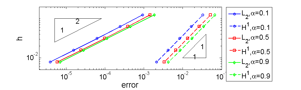
Figure 1. Error plots for smooth initial data, Example (a): $\alpha=0.1,0.5,0.9$ at $t=0.1$.

Intermediate smooth data: example (b).

In this example the initial data $v(x)$ is in $H_{0}^{1}(\Omega)$ and the numerical results are shown in Table 5 The slopes of the error curves in a log-log scale are $2$ and $1$ respectively for $L_{2}$- and $H^{1}$-norm of the errors, which agrees well with the theory for the intermediate case [6].

Table 5. Intermediate case (b) with $\alpha=0.5$ at $t=0.1$.

$h$	$1/8$	$1/16$	$1/32$	$1/64$	$1/128$	ratio	rate
$L_{2}$-error	3.04e-3	8.20e-4	2.12e-4	5.35e-5	1.32e-5	$\approx 3.97$	$O(h^{2})$
$H^{1}$-error	5.91e-2	3.09e-2	1.56e-2	7.88e-3	3.93e-3	$\approx 1.98$	$O(h)$

Nonsmooth initial data: example (c).

First in Table 6 we compare fully discrete solution $U_{h}$ via the finite difference approximation (5.1) with the semidiscrete lumped mass solution $\bar{u}_{h}$ via eigenexpansion to study the error incurred by time discretization. We observe that for each fixed spatial mesh size $h$, the difference between $\bar{u}_{h}$, the lumped mass FEM solution, and $U_{h}$ decreases with the decrease of $\tau$. In particular, for time step $\tau=10^{-6}$ the error incurred by the time discretization is negligible, so the fully discrete solutions $U_{h}$ could well be used as reference solutions.

Table 6. The difference $\bar{u}_{h}-U_{h}$, nonsmooth initial data, example (c): $\alpha=0.5$, $t=0.1$

Time step	$h$	$1/8$	$1/16$	$1/32$	$1/64$	$1/128$
$\tau=10^{-2}$	$L_{2}$-norm	2.03e-3	2.01e-3	2.00e-3	2.00e-3	2.00e-3
	$H^{1}$-norm	9.45e-3	9.17e-3	9.10e-3	9.08e-3	9.07e-3
$\tau=10^{-4}$	$L_{2}$-norm	1.81e-5	1.79e-5	1.79e-5	1.79e-5	1.79e-5
	$H^{1}$-norm	8.47e-5	8.22e-5	8.15e-5	8.13e-5	8.13e-5
$\tau=10^{-6}$	$L_{2}$-norm	1.80e-7	1.78e-7	1.78e-7	1.78e-7	1.78e-7
	$H^{1}$-norm	8.42e-7	8.17e-7	8.10e-7	8.10e-7	8.09e-7

In Table 7 and Figure 2 we present the numerical results for problem (c). These numerical results fully confirm the theoretically predicted rates for nonsmooth initial data.

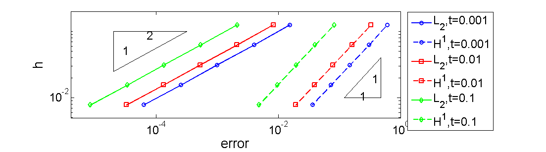
Figure 2. Error plots for lumped FEM for nonsmooth initial data, Example (c): $\alpha=0.5$.

Table 7. Error for the lumped FEM for nonsmooth initial data, example (c): $\alpha=0.5$

Time	$h$	$1/8$	$1/16$	$1/32$	$1/64$	$1/128$	ratio	rate
$t=0.001$	$L_{2}$-norm	1.55e-2	3.99e-3	1.00e-3	2.52e-4	6.26e-5	$\approx 4.01$	$O(h^{2})$
	$H^{1}$-norm	6.05e-1	3.05e-1	1.48e-1	7.29e-2	3.61e-2	$\approx 2.00$	$O(h)$
$t=0.01$	$L_{2}$-norm	8.27e-3	2.10e-3	5.28e-4	1.32e-4	3.29e-5	$\approx 4.01$	$O(h^{2})$
	$H^{1}$-norm	3.32e-1	1.61e-1	7.90e-2	3.90e-2	1.93e-2	$\approx 2.02$	$O(h)$
$t=0.1$	$L_{2}$-norm	2.12e-3	5.36e-4	1.34e-4	3.36e-5	8.43e-6	$\approx 3.99$	$O(h^{2})$
	$H^{1}$-norm	8.23e-2	4.01e-2	1.96e-2	9.72e-3	4.84e-3	$\approx 2.01$	$O(h)$

Very weak data: example (d).

The empirical convergence rate for the weak data $\delta_{\Gamma}$ agrees well with the theoretically predicted convergence rate in Theorem 3.1, which gives a ratio of $2.82$ and $1.41$, respectively, for the $L_{2}$- and $H^{1}$-norm of the error; see Table 9. Interestingly, for the standard Galerkin scheme, the $L_{2}$-norm of the error exhibits super-convergence; see Table 8.

Table 8. Error for standard FEM: initial data Dirac $\delta$-function, $\alpha=0.5$

Time	$h$	$1/8$	$1/16$	$1/32$	$1/64$	$1/128$	ratio	rate
$t=0.001$	$L_{2}$-norm	5.37e-2	1.56e-2	4.40e-3	1.23e-3	3.41e-4	$\approx 3.57$	$O(h^{1.84})$
	$H^{1}$-norm	2.68e0	1.76e0	1.20e0	8.21e-1	5.68e-1	$\approx 1.45$	$O(h^{\frac{1}{2}})$
$t=0.01$	$L_{2}$-norm	2.26e-2	6.20e-3	1.67e-3	4.46e-4	1.19e-4	$\approx 3.74$	$O(h^{1.90})$
	$H^{1}$-norm	9.36e-1	5.90e-1	3.92e-1	2.65e-1	1.84e-1	$\approx 1.46$	$O(h^{\frac{1}{2}})$
$t=0.1$	$L_{2}$-norm	8.33e-3	2.23e-3	5.90e-3	1.55e-3	4.10e-4	$\approx 3.77$	$O(h^{1.91})$
	$H^{1}$-norm	3.08e-1	1.91e-1	1.26e-1	8.44e-2	5.83e-2	$\approx 1.46$	$O(h^{\frac{1}{2}})$

Table 9. Error for lumped mass FEM: initial data Dirac $\delta$-function, $\alpha=0.5$

Time	$h$	$1/8$	$1/16$	$1/32$	$1/64$	$1/128$	ratio	rate
$t=0.001$	$L_{2}$-norm	1.98e-1	7.95e-2	3.00e-2	1.09e-2	3.95e-3	$\approx 2.75$	$O(h^{\frac{3}{2}})$
	$H^{1}$-norm	5.56e0	4.06e0	2.83e0	2.02e0	1.41e0	$\approx 1.42$	$O(h^{\frac{1}{2}})$
$t=0.01$	$L_{2}$-norm	6.61e-2	2.56e-2	9.51e-3	3.47e-3	1.25e-3	$\approx 2.78$	$O(h^{\frac{3}{2}})$
	$H^{1}$-norm	1.84e0	1.30e0	9.10e-1	6.40e-1	4.47e-1	$\approx 1.42$	$O(h^{\frac{1}{2}})$
$t=0.1$	$L_{2}$-norm	2.15e-2	8.13e-3	3.01e-3	1.09e-3	3.95e-4	$\approx 2.75$	$O(h^{\frac{3}{2}})$
	$H^{1}$-norm	5.87e-1	4.14e-1	2.88e-1	2.03e-1	1.41e-1	$\approx 1.43$	$O(h^{\frac{1}{2}})$

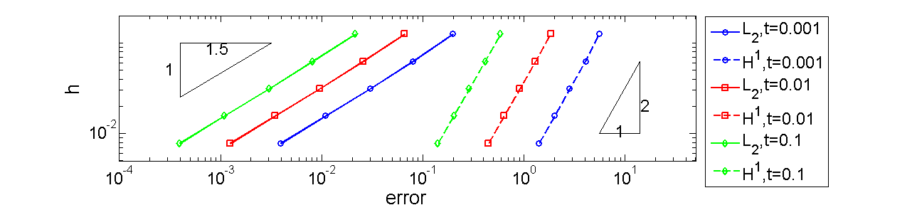
Figure 3. Error plots for Example (d): initial data Dirac $\delta$-function, $\alpha=0.5$.

References

• [1] J.-P. Bouchaud and A. Georges. Anomalous diffusion in disordered media: statistical mechanisms, models and physical applications. Phys. Rep., 195(4-5):127–293, 1990.
• [2] J. H. Bramble and J. Xu. Some estimates for a weighted $L^{2}$ projection. Math. Comp., 56(194):463–476, 1991.
• [3] P. Chatzipantelidis, R. Lazarov, and V. Thomee. Some error estimates for the finite volume element method for a parabolic problem. arXiv:1208-3219, 2012.
• [4] J. Cheng, J. Nakagawa, M. Yamamoto, and T. Yamazaki. Uniqueness in an inverse problem for a one-dimensional fractional diffusion equation. Inverse Problems, 25(11):115002, 1–16, 2009.
• [5] L. Debnath. Recent applications of fractional calculus to science and engineering. Int. J. Math. Math. Sci., 54:3413–3442, 2003.
• [6] B. Jin, R. Lazarov, and Z. Zhou. Error estimates for a semidiscrete finite element method for fractional order parabolic equations. Technical report, Texas A&M University, April 2012. (see, arXiv:1204-3804).
• [7] B. Jin and X. Lu. Numerical identification of a Robin coefficient in parabolic problems. Math. Comput., 81(279):1369–1398, 2012.
• [8] Y. L. Keung and J. Zou. Numerical identifications of parameters in parabolic systems. Inverse Problems, 14(1):83–100, 1998.
• [9] A. Kilbas, H. Srivastava, and J. Trujillo. Theory and Applications of Fractional Differential Equations. Elsevier, Amsterdam, 2006.
• [10] Y. Lin and C. Xu. Finite difference/spectral approximations for the time-fractional diffusion equation. J. Comput. Phys., 225(2):1533–1552, 2007.
• [11] I. Podlubny. Fractional Differential Equations. Academic Press, San Diego, CA, 1999.
• [12] K. Sakamoto and M. Yamamoto. Initial value/boundary value problems for fractional diffusion-wave equations and applications to some inverse problems. J. Math. Anal. Appl., 382(1):426–447, 2011.
• [13] H. Seybold and R. Hilfer. Numerical algorithm for calculating the generalized Mittag-Leffler function. SIAM J. Numer. Anal., 47(1):69–88, 2008/09.
• [14] V. Thomée. Galerkin Finite Element Methods for Parabolic Problems, volume 25 of Springer Series in Computational Mathematics. Springer-Verlag, Berlin, 1997.