On the Initial Value Problem for
Causal Variational Principles

Abstract.

We formulate the initial value problem for causal variational principles in the continuous setting on a compact metric space. The existence and uniqueness of solutions is analyzed. The results are illustrated by simple examples.

1. Introduction

Causal variational principles arise in the context of relativistic quantum theory (see the survey article [5] and the references therein). In [3] they were introduced from a mathematical perspective, and the existence of minimizers has been proven in various situations. A more detailed analysis of causal variational principles and of the corresponding Euler-Lagrange equations is carried out in [6, 2].

In the present paper, we analyze the question how an initial value problem can be posed for causal variational principles, and whether it has a unique solution. For technical simplicity, we restrict attention to the so-called continuous setting on a compact manifold as introduced in [3, Section 1.4] and more generally in [6]. But using the techniques in [2], many methods and results could be extended in a straightforward way to the non-compact setting. Since we shall not make use of the manifold structure, we now let ${\mathscr{F}}$ be a compact metric space. For a given Lagrangian ${\mathcal{L}}\in C^{0}({\mathscr{F}}\times{\mathscr{F}},\mathbb{R}^{+}_{0})$ which is symmetric (i.e. ${\mathcal{L}}(x,y)={\mathcal{L}}(y,x)$ for all $x,y\in{\mathscr{F}}$), we introduce the action ${\mathcal{S}}$ by

$${\mathcal{S}}[\rho]=\iint_{{\mathscr{F}}\times{\mathscr{F}}}{\mathcal{L}}(x,y)\>d\rho(x)\>d\rho(y)\>.$$ (1.1)

Here $\rho$ is a normalized positive regular Borel measure on ${\mathscr{F}}$, referred to as the universal measure. Our action principle is to minimize ${\mathcal{S}}$ by varying $\rho$ in the class

$${\mathbb{M}}^{+}_{1}({\mathscr{F}}):=\{\text{normalized positive regular Borel measures on~{}${\mathscr{F}}$}\}\>.$$ (1.2)

For a minimizer $\rho$, space-time is defined as the support of $\rho$,

$$M:=\operatorname{supp}\rho\subset{\mathscr{F}}\>.$$

A-priori, $M$ is a topological space (carrying the relative topology of ${\mathscr{F}}$). Additional structures, like the following causal structure, are induced on $M$ by the Lagrangian.

Definition 1.1.

Two space-time points $x,y\in M$ are called time-like separated if ${\mathcal{L}}(x,y)>0$. They are called space-like separated if ${\mathcal{L}}(x,y)=0$.

For more space-time structures in the richer context of causal fermion systems we refer to [5, 4].

For the following concepts, it is important to keep in mind that space-time is not a-priori given, but emerges by minimizing the causal action. When varying $\rho$, one also varies space-time together with all the additional space-time structures. This situation can be understood similar as in general relativity, where the space-time manifold with its Lorentzian metric and causal structure are not a-priori given, but are obtained dynamically by solving the Einstein equations.

When solving the classical Cauchy problem, instead of searching for a global solution, it is often easier to look for a local solution around a given initial value surface. This concept of a local solution also reflects the common physical situation where the physical system under consideration is only a small subsystem of the whole universe. With this in mind, our first step is to “localize” our variational principle by introducing the so-called inner variational principle. To this end, we fix a Borel subset ${\mathfrak{I}}\subset{\mathscr{F}}$ (the “inner system”) and minimize the action

$${\mathcal{S}}_{\mathfrak{I}}[\rho,\phi]:=\iint_{{\mathfrak{I}}\times{\mathfrak{I}}}{\mathcal{L}}(x,y)\>d\rho(x)\>d\rho(y)+2\int_{{\mathfrak{I}}}(\phi(x)-{\mathfrak{s}})\>d\rho(x)$$ (1.3)

under variations in the class

$${\mathbb{M}}^{+}({\mathfrak{I}}):=\{\text{bounded positive regular Borel measures on~{}${\mathfrak{I}}$}\}\>,$$ (1.4)

where ${\mathfrak{s}}>0$ is a parameter, and $\phi$ is a non-negative function in the class

$${\mathbb{B}}^{+}({\mathfrak{I}}):=\big{\{}\phi:{\mathfrak{I}}\rightarrow\mathbb{R}^{+}_{0}\,\big{|}\,\text{$\phi$ bounded and lower semi-continuous}\big{\}}\>.$$ (1.5)

The derivation of the inner variational principle will be given in Section 2.1. Here we only explain the basic concepts behind the inner variational principle. First, it is important to observe that the causal variational principle (1.1) is non-local in the sense that ${\mathcal{L}}(x,y)$ may be non-zero even for points $x,y$ which are are far apart. This means that the subsystem ${\mathfrak{I}}$ will be influenced also by the universal measure outside this subsystem. This effect is taken into account in (1.3) by the function $\phi$, referred to as the external potential. The parameter ${\mathfrak{s}}$, on the other hand, plays the role of a Lagrange multiplier that takes care of the volume constraint in (1.2) (note that the measure in (1.2) is normalized, whereas the measure in (1.4) is not).

The external potential is closely linked to our concept for prescribing initial values, as we now explain. In the setting of causal variational principles, initial values are introduced naturally by prescribing a measure $\rho_{0}\in{\mathbb{M}}^{+}({\mathfrak{I}})$ (the “initial data”) and by demanding that $\rho\geq\rho_{0}$. If we implemented the inequality $\rho\geq\rho_{0}$ as a side condition for the inner variational principle, treating the inequality constraint with Lagrange multipliers would give rise to additional terms in the EL equations. This means that the EL equations would depend on the initial data, in clear contrast to the usual concept of solving a-priori given EL equations for prescribed initial data. For this reason, imposing the side condition $\rho\geq\rho_{0}$ is not a sensible concept. It is preferable to minimize (1.3) without constraints, but to choose $\phi$ in such a way that the minimizing measure $\rho$ satisfies the inequality $\rho\geq\rho_{0}$. This leads to the following definition.

Definition 1.2.

Given a measure $\rho_{0}\in{\mathbb{M}}^{+}({\mathfrak{I}})$ and a parameter ${\mathfrak{s}}>0$, a measure $\rho\in{\mathbb{M}}^{+}({\mathfrak{I}})$ is called a solution of the initial value problem in ${\mathfrak{I}}$ with initial data $\rho_{0}$ and external potential $\phi\in{\mathbb{B}}^{+}({\mathfrak{I}})$ if it is a minimizer of the inner variational principle with the additional property $\rho\geq\rho_{0}$. We denote the set of solutions together with the corresponding external potentials by

$$\mathfrak{S}_{\mathfrak{I}}(\rho_{0})=\big{\{}(\rho,\phi)\,\big{|}\,\text{$\rho$ solves the initial value problem with external potential~{}$\phi$}\big{\}}\,.$$ (1.6)

A detailed discussion of our method for prescribing initial data will be given in Section 2.3.

Note that in the above definition, the external potential can be chosen arbitrarily up to the requirement that the corresponding solution of the inner variational principle should comply with the initial data. Following the concept that the external potential describes the influence of the outer system, choosing $\phi$ can be viewed as suitably “preparing” the outer system in such a way that the resulting universal measure is compatible with the initial data. Since we cannot expect that there is a unique way of preparing the outer system, there may be a whole family of possible choices of $\phi$. As the outer system is unknown for principal reasons, the choice of $\phi$ is not determined a-priori, and it is not unique. As an example, for a given minimizer $(\phi,\rho)$, increasing the external potential outside the support of $\rho$ does not change the action (1.3) and clearly preserves the minimizing property of a measure $\rho$. As an additional difficulty, even for a fixed external potential, in general there will be no unique minimizing measure $\rho$. Despite these complications, we succeed in constructing a uniquely defined so-called domain of dependence on which the minimizing measure $\rho$ is unique for any choice of $\phi$. Moreover, we construct a so-called maximal optimal solution where both $\rho$ and $\phi|_{\operatorname{supp}\rho}$ are uniquely determined by suitably “optimizing” the external potential.

The paper is organized as follows. In Section 2, we derive the inner variational principle as well as the corresponding Euler-Lagrange equations. Moreover, we discuss our method of prescribing initial data and introduce different notions of optimal solutions. In Section 3, we prove existence results for the inner variational principle. Moreover, we characterize those initial data which admit solutions of the initial value problem, and we prove existence of optimal solutions. In Section 4, we introduce the domain of dependence as the largest set where the inner variational principle has a unique solution for every $\phi\in{\mathbb{B}}^{+}({\mathfrak{I}})$. Furthermore, we analyze the uniqueness of optimal solutions and construct the uniquely determined maximal optimal solution. Finally, Section 5 provides some simple yet instructive examples of initial value problems.

2. Setting up the Initial Value Problem

2.1. The Inner Variational Principle

The universal measure $\rho$ in (1.1) should be regarded as describing the whole space-time. In most applications, however, one is interested only in a subregion of space-time whose volume is much smaller than the total volume of space-time. In order to describe this situation, we now “localize” the variational principle (1.1) as follows. By rescaling the measure $\rho$ we arrange that $\rho({\mathscr{F}})=V$ with $V>0$ (this is useful because we will later take the infinite volume limit $V\rightarrow\infty$). Moreover, we fix a Borel subset ${\mathfrak{I}}\subset{\mathscr{F}}$ (the inner system) and decompose the measure $\rho$ as

$$\rho=\rho_{\text{in}}+\rho_{\text{out}}$$

with $\rho_{\text{in}}=\chi_{\mathfrak{I}}\,\rho$ and $\rho_{\text{out}}=\chi_{{\mathscr{F}}\setminus{\mathfrak{I}}}\,\rho$ (and $\chi$ denotes the characteristic function). We also set $V_{\text{in}}=\rho_{\text{in}}({\mathscr{F}})=\rho({\mathfrak{I}})$ and $V_{\text{out}}=\rho_{\text{out}}({\mathscr{F}})$; clearly $V=V_{\text{in}}+V_{\text{out}}$. The action (1.1) becomes

$${\mathcal{S}}[\rho]={\mathcal{S}}[\rho_{\text{in}}]+{\mathcal{S}}[\rho_{\text{out}}]+2\iint_{{\mathscr{F}}\times{\mathscr{F}}}{\mathcal{L}}(x,y)\>d\rho_{\text{in}}(x)\>d\rho_{\text{out}}(y)\>.$$ (2.1)

We have the situation in mind that only $\rho_{\text{in}}$ is known, whereas the measure $\rho_{\text{out}}$ in the “outer system” ${\mathscr{F}}\setminus{\mathfrak{I}}$ is inaccessible to the physical system under consideration. This means that, in order to derive the effective action principle of the inner system, we only consider variations of the measure $\rho_{\text{in}}$. It is important to notice that the volume $\rho_{\text{in}}({\mathscr{F}})$ need not be preserved in the variation, as only the total volume of the whole space-time must be kept fixed. The latter can be arranged by rescaling $\rho_{\text{out}}$. Thus for a variation $\tilde{\rho}_{\text{in}}$ of $\rho_{\text{in}}$ we consider the corresponding variation of $\rho$ as given by

$$\tilde{\rho}=\tilde{\rho}_{\text{in}}+\frac{V-\tilde{V}_{\text{in}}}{V_{\text{out}}}\>\rho_{\text{out}}\>,$$

where we impose that $\operatorname{supp}\tilde{\rho}_{\text{in}}\subset{\mathfrak{I}}$ and set $\tilde{V}_{\text{in}}:=\tilde{\rho}_{\text{in}}({\mathscr{F}})$. The corresponding action (2.1) becomes

$${\mathcal{S}}[\tilde{\rho}]={\mathcal{S}}[\tilde{\rho}_{\text{in}}]+\Big{(}\frac{V-\tilde{V}_{\text{in}}}{V_{\text{out}}}\Big{)}^{2}\>{\mathcal{S}}[\rho_{\text{out}}]+2\>\frac{V-\tilde{V}_{\text{in}}}{V_{\text{out}}}\iint_{{\mathscr{F}}\times{\mathscr{F}}}{\mathcal{L}}(x,y)\>d\tilde{\rho}_{\text{in}}(x)\>d\rho_{\text{out}}(y)\>.$$

We now consider the limiting case when the total volume $V\rightarrow\infty$, whereas $V_{\text{in}}$ and $\tilde{V}_{\text{in}}$ stay bounded. Moreover, we assume that ${\mathcal{S}}[\rho_{\text{out}}]$ grows linearly in $V_{\text{out}}$, so that the following limits exist,

$$\phi(x) :=\lim_{V_{\text{out}}\rightarrow\infty}\int_{\mathscr{F}}{\mathcal{L}}(x,y)\>d\rho_{\text{out}}(y)\in C^{0}({\mathfrak{I}},\mathbb{R}^{+}_{0})$$

$${\mathfrak{s}} :=\lim_{V_{\text{out}}\rightarrow\infty}\frac{{\mathcal{S}}[\rho_{\text{out}}]}{V_{\text{out}}}\>.$$

Under these assumptions, our action converges after subtracting an irrelevant constant,

$$\lim_{V\rightarrow\infty}\Big{(}{\mathcal{S}}[\tilde{\rho}]-{\mathcal{S}}[\rho_{\text{out}}]\Big{)}={\mathcal{S}}[\tilde{\rho}_{\text{in}}]+2\int_{{\mathfrak{I}}}\phi(x)\>d\tilde{\rho}_{\text{in}}-2\,\tilde{V}_{\text{in}}\>{\mathfrak{s}}\>.$$

To simplify the notation, we again denote the measure $\tilde{\rho}_{\text{in}}$ by $\rho$. We then obtain the action (1.3), which is to be minimized under variations in the class (1.4). This variational principle can be regarded as a generalization of our original action principle (1.1) and (1.2), where we replaced the normalization constraint in (1.2) by the Lagrange multiplier term $-2{\mathfrak{s}}\rho({\mathfrak{I}})$. As indicated in the introduction, the influence of the universal measure in the outer system is described effectively in the inner action (1.3) by the external potential $\phi$. In view of our later constructions, it is useful to allow the external potential to be in the larger class ${\mathbb{B}}^{+}({\mathfrak{I}})$ of lower semi-continuous functions (see (1.5)).

Obviously, in the case ${\mathfrak{s}}<0$ the variational principle only has the trivial minimizer $\rho=0$. In the case ${\mathfrak{s}}=0$, every minimizing measure is supported on the zero set of $\phi$, and restricting attention to measures with this property, the action (1.3) reduces to (1.1). In order to rule out these trivial cases, we shall always assume that ${\mathfrak{s}}>0$. We thus obtain the following variational principle.

Definition 2.1.

Let ${\mathfrak{I}}$ be a metric space and ${\mathcal{L}}\in C^{0}({\mathfrak{I}}\times{\mathfrak{I}},\mathbb{R}^{+}_{0})$ a symmetric Lagrangian. Given a parameter ${\mathfrak{s}}>0$ and a function $\phi\in{\mathbb{B}}^{+}({\mathfrak{I}})$, the inner variational principle is to minimize the functional ${\mathcal{S}}_{\mathfrak{I}}$ in (1.3) under variations of $\rho$ in the class ${\mathbb{M}}^{+}({\mathfrak{I}})$.

We will see in Section 3.2 that the inner variational principle has solutions for any ${\mathfrak{s}}>0$ and $\phi\in{\mathbb{B}}^{+}({\mathfrak{I}})$.

2.2. The Euler-Lagrange Equations

In this section, we derive the Euler-Lagrange (EL) equations corresponding to the inner variational principle. For a convenient notation, we set

$${\mathbb{M}}({\mathfrak{I}}):=\{\text{bounded signed regular Borel measures on ${\mathfrak{I}}$}\}$$

and introduce the short notations

$${\mathcal{L}}\mu(x) =\int_{\mathfrak{I}}{\mathcal{L}}(x,y)\>d\mu(y)$$

$$\langle f,\mu\rangle =\int_{\mathfrak{I}}f(x)\>d\mu(x)\>,$$

where $\mu\in{\mathbb{M}}({\mathfrak{I}})$ is any signed measure and $f:{\mathfrak{I}}\rightarrow\mathbb{R}$ a measurable function. Then the action ${\mathcal{S}}_{\mathfrak{I}}$ can be written in the compact form

$${\mathcal{S}}_{\mathfrak{I}}[\rho,\phi]=\langle{\mathcal{L}}\rho,\rho\rangle+2\,\langle\phi-{\mathfrak{s}},\rho\rangle\>.$$ (2.2)

In order to further simplify the setting, we note that the action (1.3) is invariant under the rescaling

$$\phi\rightarrow\lambda\,\phi\>,\qquad\rho\rightarrow\lambda\,\rho\>,\qquad{\mathfrak{s}}\rightarrow\lambda\,{\mathfrak{s}}\>,\qquad{\mathcal{S}}_{\mathfrak{I}}\rightarrow\lambda^{-2}\>{\mathcal{S}}_{\mathfrak{I}}\qquad(\text{where~{}$\lambda>0$})\>.$$ (2.3)

With this rescaling, we can always arrange that ${\mathfrak{s}}=1$.

In the next proposition we use similar methods as in [6, Section 3.1].

Proposition 2.2.

(Euler-Lagrange Equations) Every minimizer $\rho$ of the inner variational principle has the properties

$${\mathcal{L}}\rho+\phi\big{|}_{\operatorname{supp}\rho}\equiv\min_{\mathfrak{I}}\big{(}{\mathcal{L}}\rho+\phi\big{)}=1\quad\text{and}$$ (2.4)

$$\langle{\mathcal{L}}\mu,\mu\rangle\geq 0\qquad\text{for all~{}$\mu\in{\mathbb{M}}(\operatorname{supp}\rho)$}\>.$$ (2.5)

Proof.

Let $\rho\in{\mathbb{M}}^{+}({\mathfrak{I}})$ be a minimizer of the inner variational principle (1.3) with external potential $\phi\in{\mathbb{B}}^{+}({\mathfrak{I}})$. We consider the family of measures $\tilde{\rho}_{t}=\rho+t\,\delta_{x}$ with $t\geq 0$, where $\delta_{x}$ denotes the Dirac measure supported at $x\in{\mathfrak{I}}$. Taking the right-sided derivative of ${\mathcal{S}}_{\mathfrak{I}}[\tilde{\rho}_{t},\phi]$ with respect to $t$, we find that

$$({\mathcal{L}}\rho)(x)+\phi(x)-1\geq 0\qquad\text{for all~{}$x\in{\mathfrak{I}}$}\>.$$ (2.6)

Next, we consider for $t\in(-1,1)$ the family of measures $\tilde{\rho}_{t}=(1+t)\,\rho$. Again differentiating the action with respect to $t$, we find that

$$\int_{\mathfrak{I}}\big{(}({\mathcal{L}}\rho)(x)+\phi(x)-1\big{)}\>d\rho(x)=0\>.$$ (2.7)

Combining (2.6) and (2.7) gives (2.4).

In order to prove (2.5), we define the real Hilbert space $\mathscr{H}_{\rho}=L^{2}({\mathfrak{I}},d\rho)$ and the linear operator

$${\mathcal{L}}_{\rho}\>:\>\mathscr{H}_{\rho}\rightarrow\mathscr{H}_{\rho}\>,\qquad({\mathcal{L}}_{\rho}\psi)(x)=\int_{\mathfrak{I}}{\mathcal{L}}(x,y)\>\psi(y)\>d\rho(y)\>.$$ (2.8)

For any bounded function $\psi\in\mathscr{H}_{\rho}$, we consider for $t\in(-\varepsilon,\varepsilon)$ (with $0<\varepsilon<1/\|\psi\|_{\infty}$) the family of measures

$$\tilde{\rho}_{t}=(1+t\,\psi)\>\rho$$

(where $\psi\rho$ is the signed measure $(\psi\rho)(\Omega):=\int_{\Omega}\psi d\rho$). Differentiating the action twice, we obtain

$$0\leq\iint_{{\mathfrak{I}}\times{\mathfrak{I}}}{\mathcal{L}}(x,y)\>\psi(x)\,d\rho(x)\>\psi(y)\,d\rho(y)=\langle\psi,{\mathcal{L}}_{\rho}\psi\rangle_{\mathscr{H}}\>,$$

which shows that ${\mathcal{L}}_{\rho}$ is a positive semi-definite operator on $\mathscr{H}_{\rho}$. The relation (2.5) follows by approximating any given measure $\mu\in{\mathbb{M}}(\operatorname{supp}(\rho))$ by a series $(\mu_{n})$ of measures of the form $\mu_{n}=\psi_{n}\,\rho$ with $\psi_{n}\in\mathscr{H}_{\rho}$. ∎

Inserting the relation (2.4) into the action (2.2), we obtain the following result.

Corollary 2.3.

For a minimizer $\rho\in{\mathbb{M}}^{+}({\mathfrak{I}})$ of the inner variational principle with external potential $\phi\in{\mathbb{B}}^{+}({\mathfrak{I}})$, the inner action takes the value

$${\mathcal{S}}[\rho,\phi]=-\langle{\mathcal{L}}\rho,\rho\rangle=\langle\phi-1,\rho\rangle\,.$$ (2.9)

2.3. Prescribing Initial Data

To motivate our method, let us assume that we want to find a minimizer $\rho$ of the inner variational principle which has the additional property that $\rho\geq\rho_{0}$ for a given measure $\rho_{0}\in{\mathbb{M}}^{+}({\mathfrak{I}})$ (the “initial data”). The most obvious idea for implementing the constraint $\rho\geq\rho_{0}$ is to write $\rho$ in the form $\rho=\rho_{0}+\nu$ with a measure $\nu\in{\mathbb{M}}^{+}({\mathfrak{I}})$. Substituting this ansatz into (1.3), one obtains

$${\mathcal{S}}=\iint_{{\mathfrak{I}}\times{\mathfrak{I}}}{\mathcal{L}}(x,y)\>d\nu(x)\>d\nu(y)+2\int_{{\mathfrak{I}}}(\tilde{\phi}(x)-1)\>d\nu(x)+\text{const}\>,$$

where the new external potential $\tilde{\phi}$ is given by

$$\tilde{\phi}(x)=\phi(x)+\int_{\mathfrak{I}}{\mathcal{L}}(x,y)\>d\rho_{0}\>.$$

Thus one can minimize ${\mathcal{S}}$ under variations of $\nu\in{\mathbb{M}}^{+}({\mathfrak{I}})$. According to Proposition 2.2, we obtain the EL equations

$${\mathcal{L}}\nu+\tilde{\phi}\big{|}_{\operatorname{supp}\nu}\equiv\min_{\mathfrak{I}}\big{(}{\mathcal{L}}\nu+\tilde{\phi}\big{)}=1\quad\text{and}$$ (2.10)

$$\langle{\mathcal{L}}\mu,\mu\rangle\geq 0\qquad\text{for all~{}$\mu\in{\mathbb{M}}(\operatorname{supp}\nu)$}\>.$$ (2.11)

The problem is that the EL equations (2.10) and (2.11) are considerably weaker than the earlier equations for $\rho$, (2.4) and (2.5), because they must hold only on $\operatorname{supp}\nu$, but not on $\operatorname{supp}\rho$ (note that in general $\operatorname{supp}\rho\supsetneq\operatorname{supp}\nu$). For this reason, minimizing $\nu$ is not the correct procedure. Instead, our strategy is to minimize $\rho$ over the whole class ${\mathbb{M}}^{+}({\mathfrak{I}})$, but to always choose the external potential in such a way that the minimizer satisfies the constraint $\rho\geq\rho_{0}$. This leads to the initial value problem formulated in Definition 1.2 above.

For the applications, it might be useful to consider more general initial data, which consists of the measure $\rho_{0}$ and in addition of a closed subset ${\mathfrak{I}}_{0}\subset{\mathfrak{I}}$. We demand that the conditions (2.4) and (2.5) also hold on the set ${\mathfrak{I}}_{0}$.

Definition 2.4.

Given a measure $\rho_{0}\in{\mathbb{M}}^{+}({\mathfrak{I}})$ and a closed set ${\mathfrak{I}}_{0}\subset{\mathfrak{I}}$, a measure $\rho\in{\mathbb{M}}^{+}({\mathfrak{I}})$ is called a solution of the initial value problem in ${\mathfrak{I}}$ with initial data $(\rho_{0},{\mathfrak{I}}_{0})$ and external potential $\phi\in{\mathbb{B}}^{+}({\mathfrak{I}})$ if it is a minimizer of the inner variational principle with the following additional properties:

• $\rho\geq\rho_{0}$
  

• ${\mathcal{L}}\rho+\phi\big{|}_{{\mathfrak{I}}_{0}}\equiv 1$

• $\displaystyle\langle{\mathcal{L}}\mu,\mu\rangle\geq 0\qquad\text{for all~{}$\mu\in{\mathbb{M}}({\mathfrak{I}}_{0}\cup\operatorname{supp}\rho)$}$ .

In analogy to (1.6), we denote the set of solutions by $\mathfrak{S}_{\mathfrak{I}}(\rho_{0},{\mathfrak{I}}_{0})$.

The initial value problem in Definitions 1.2 and 2.4 cannot be solved for arbitrarily chosen initial data $(\rho_{0},{\mathfrak{I}}_{0})$. For example, if the measure $\rho_{0}$ is chosen such that there is a point $x\in\operatorname{supp}(\rho_{0})$ with $({\mathcal{L}}\rho_{0})(x)>1$, then the EL equation (2.4) excludes existence of a minimizer $\rho\in{\mathbb{M}}^{+}({\mathfrak{I}})$ with $\rho\geq\rho_{0}$ for any external potential. In Section 3.3 we will characterize those initial data which admit solutions of the initial value problem.

2.4. Optimizing the External Potential

Let us assume that the initial data $\rho_{0}$ or $(\rho_{0},{\mathfrak{I}}_{0})$ admits a solution $(\rho,\phi)$ of the initial value problem. Then this solution will in general not be unique. Moreover, there is an arbitrariness in choosing the external potential. Our strategy for getting uniqueness is to choose the external potential in an “optimal way”. There are three basic notions of optimality:

$$\begin{array}[]{cl}\text{(A)}&\text{Minimize the action~{}${\mathcal{S}}_{\mathfrak{I}}[\rho,\phi]$, where~{}$(\rho,\phi)\in\mathfrak{S}_{\mathfrak{I}}(\rho_{0},{\mathfrak{I}}_{0})$.}\\[1.99997pt] \text{(B)}&\text{Minimize the value of~{}$\max_{\operatorname{supp}(\rho)}\phi$, where~{}$(\rho,\phi)\in\mathfrak{S}_{\mathfrak{I}}(\rho_{0},{\mathfrak{I}}_{0})$.}\\[1.99997pt] \text{(C)}&\text{Maximize the volume~{}$\rho({\mathfrak{I}})$, where~{}$(\rho,\phi)\in\mathfrak{S}_{\mathfrak{I}}(\rho_{0},{\mathfrak{I}}_{0})$.}\end{array}$$ (2.12)

For clarity, we note that whether to maximize or to minimize in the above optimization problems is determined by the requirement to avoid trivial minimizers. Namely, if we had taken the reverse choice in any of the problems (A)–(C), one verifies immediately from (2.4) and (2.9) as well as from the condition $\rho\geq\rho_{0}$ that the measure $\rho=\rho_{0}$ would be a trivial solution.

Solutions exist for all of the optimization problems in (2.12) (see Theorem 3.15 in Section 3.4), but neither $\rho$ nor $\phi$ are unique in general (cf. the examples in Section 5). Therefore, we propose another notion of optimality by first maximizing the volume and then maximizing the action:

$$\text{(D)}\quad\text{Maximize the action~{}${\mathcal{S}}_{\mathfrak{I}}[\rho,\phi]$ in $\mathfrak{S}_{{\mathfrak{I}}}^{\text{maxV}}(\rho_{0},{\mathfrak{I}}_{0})$}\>,$$ (2.13)

where $\mathfrak{S}_{{\mathfrak{I}}}^{\text{maxV}}(\rho_{0},{\mathfrak{I}}_{0})$ is defined as the set of solutions of the initial value problem with maximal volume,

$$\mathfrak{S}_{{\mathfrak{I}}}^{\text{maxV}}(\rho_{0},{\mathfrak{I}}_{0}):=\bigg{\{}(\rho,\phi)\in\mathfrak{S}_{\mathfrak{I}}\,\Big{|}\,\rho({\mathfrak{I}})=\max_{(\tilde{\rho},\tilde{\phi})\in\mathfrak{S}_{\mathfrak{I}}}\tilde{\rho}({\mathfrak{I}})\bigg{\}}\>.$$

In Section 4.2 we will prove that solving the optimization problem (D) in suitable space-time regions will indeed give a unique solution of the initial value problem. This analysis will also explain why in (D) we must maximize (and not minimize) the action.

3. Existence Results

We now enter the analysis of the inner variational principle and of solutions of the initial value problem. We always keep $\rho_{0}\in{\mathbb{M}}^{+}({\mathfrak{I}})$ fixed and use the rescaling (2.3) to set ${\mathfrak{s}}=1$. For the existence results in this section we need to assume that the inner system ${\mathfrak{I}}$ is a closed subset of ${\mathscr{F}}$ and that the Lagrangian ${\mathcal{L}}$ is strictly positive on the diagonal,

$${\mathcal{L}}(x,x)>0\qquad\text{for all~{}$x\in{\mathfrak{I}}$}\>.$$ (3.1)

3.1. Preparatory Considerations

The following simple observation makes it possible to construct new minimizers from a given minimizer of the inner variational principle.

Lemma 3.1.

Suppose that $\rho$ is a minimizer of ${\mathcal{S}}_{\mathfrak{I}}$ with external potential $\phi\in{\mathbb{B}}^{+}({\mathfrak{I}})$. Then any measure $\tilde{\rho}\in{\mathbb{M}}^{+}({\mathfrak{I}})$ with $\tilde{\rho}\leq\rho$ is a minimizer of ${\mathcal{S}}_{\mathfrak{I}}$ with external potential $\tilde{\phi}\in{\mathbb{B}}^{+}({\mathfrak{I}})$ given by

$$\tilde{\phi}(x)=\phi(x)+\int_{\mathfrak{I}}{\mathcal{L}}(x,y)\>d(\rho-\tilde{\rho})(y)\>.$$

Proof.

We first note that

$${\mathcal{L}}\tilde{\rho}(x)+\tilde{\phi}(x)-1=({\mathcal{L}}\rho)(x)+\phi(x)-1=0\quad\text{for all }x\in\operatorname{supp}\rho\,.$$

Setting $\mu:=\rho-\tilde{\rho}\in{\mathbb{M}}^{+}(\operatorname{supp}\rho)$, we then find that

$${\mathcal{S}}_{\mathfrak{I}}[\rho,\tilde{\phi}] ={\mathcal{S}}_{\mathfrak{I}}[\tilde{\rho}+\mu,\tilde{\phi}]={\mathcal{S}}_{\mathfrak{I}}[\tilde{\rho},\tilde{\phi}]+2\langle{\mathcal{L}}\tilde{\rho},\mu\rangle+\langle{\mathcal{L}}\mu,\mu\rangle+2\langle\tilde{\phi}-1,\mu\rangle$$

$$\geq{\mathcal{S}}_{\mathfrak{I}}[\tilde{\rho},\tilde{\phi}]+2\langle{\mathcal{L}}\tilde{\rho}+\tilde{\phi}-1,\mu\rangle={\mathcal{S}}_{\mathfrak{I}}[\tilde{\rho},\tilde{\phi}]\,.$$

Thus for any $\nu\in{\mathbb{M}}^{+}({\mathfrak{I}})$,

$${\mathcal{S}}_{\mathfrak{I}}[\tilde{\rho},\tilde{\phi}]\leq{\mathcal{S}}_{\mathfrak{I}}[\rho,\tilde{\phi}]={\mathcal{S}}_{\mathfrak{I}}[\rho,\phi]+2\langle{\mathcal{L}}(\rho-\tilde{\rho}),\rho\rangle\leq{\mathcal{S}}_{\mathfrak{I}}[\nu,\phi]+2\langle{\mathcal{L}}(\rho-\tilde{\rho}),\rho\rangle\leq{\mathcal{S}}_{\mathfrak{I}}[\nu,\tilde{\phi}]\,,$$

where we used that $\rho$ is a minimizer of ${\mathcal{S}}_{\mathfrak{I}}[\,.\,,\phi]$ and that $\phi\leq\tilde{\phi}$. We conclude that $\tilde{\rho}$ is a minimizer of ${\mathcal{S}}_{\mathfrak{I}}[\,.\,,\tilde{\phi}]$. ∎

The previous lemma is particularly useful for “localizing” a solution in a closed subset of ${\mathfrak{I}}$:

Corollary 3.2.

Suppose that $\rho$ is a minimizer of ${\mathcal{S}}_{\mathfrak{I}}$ with external potential $\phi$. Choosing a closed subset ${\mathscr{J}}\subset{\mathfrak{I}}$, we set

$$\tilde{\rho}=\chi_{{\mathscr{J}}}\,\rho\qquad\text{and}\qquad\tilde{\phi}(x)=\phi(x)+\int_{{\mathfrak{I}}\setminus{\mathscr{J}}}{\mathcal{L}}(x,y)\>d\rho(y)\>.$$

Then $\tilde{\rho}$ is a minimizer of ${\mathcal{S}}_{\mathfrak{I}}$ with external potential $\tilde{\phi}$.

The next simple estimate gives some information on the support of a minimizing measure.

Lemma 3.3.

Let $\rho$ be a minimizer of ${\mathcal{S}}_{\mathfrak{I}}$ with external potential $\phi$. Then

$$\operatorname{supp}\rho\subseteq\{x\in{\mathfrak{I}}\>|\>\phi(x)\leq 1\}\>.$$

Proof.

Assume conversely that there is $\varepsilon>0$ and a set $U\subset{\mathfrak{I}}$ with $\rho(U)>0$ and $\phi|_{U}\geq 1+\varepsilon$. Then

$${\mathcal{S}}_{\mathfrak{I}}[\chi_{{\mathfrak{I}}\setminus U}\,\rho,\phi] =\langle\chi_{{\mathfrak{I}}\setminus U}\,\rho,{\mathcal{L}}\,\chi_{{\mathfrak{I}}\setminus U}\,\rho\rangle+2\,\langle(\phi-1_{\mathfrak{I}}),\chi_{{\mathfrak{I}}\setminus U}\,\rho\rangle$$

$$\leq\langle{\mathcal{L}}\rho,\rho\rangle+2\int_{{\mathfrak{I}}\setminus U}(\phi-1)\,d\rho$$

$$={\mathcal{S}}_{\mathfrak{I}}[\rho,\phi]-2\int_{U}(\phi-1)\,d\rho\leq{\mathcal{S}}_{\mathfrak{I}}[\rho,\phi]-2\,\varepsilon\,\rho(U)<{\mathcal{S}}_{\mathfrak{I}}[\rho,\phi]\>,$$

in contradiction to the minimality of $\rho$. ∎

A similar estimate allows us to modify the external potential while preserving the minimizing property of $\rho$.

Lemma 3.4.

Let $\rho$ be a minimizer of ${\mathcal{S}}_{\mathfrak{I}}$ with external potential $\phi$. Then $\rho$ is also a minimizer of ${\mathcal{S}}_{\mathfrak{I}}$ if the external potential is replaced by any function $\tilde{\phi}\in{\mathbb{B}}^{+}({\mathfrak{I}})$ with the properties

$$\left\{\begin{array}[]{ll}\tilde{\phi}(x)=\phi(x)&\text{if $x\in\operatorname{supp}(\rho)$}\\[1.99997pt] \tilde{\phi}(x)\geq\min\big{(}\phi(x),1\big{)}&\text{if $x\not\in\operatorname{supp}(\rho)$}\>.\end{array}\right.$$

Proof.

Let $U=\{x\in{\mathfrak{I}}\>|\>\phi(x)<1\}$. Then for every $\tilde{\rho}\in{\mathbb{M}}^{+}({\mathfrak{I}})$,

$${\mathcal{S}}_{\mathfrak{I}}[\rho,\tilde{\phi}]={\mathcal{S}}_{\mathfrak{I}}[\rho,\phi]\leq{\mathcal{S}}_{\mathfrak{I}}[\chi_{U}\tilde{\rho},\phi]\>,$$

where we used that $\phi$ and $\tilde{\phi}$ coincide on the support of $\rho$ and that $\rho$ is a minimizer. Next, we know by assumption that on the set $U$, the inequality $\phi\leq\tilde{\phi}$ holds, and thus

$${\mathcal{S}}_{\mathfrak{I}}[\chi_{U}\tilde{\rho},\phi]\leq{\mathcal{S}}_{\mathfrak{I}}[\chi_{U}\tilde{\rho},\tilde{\phi}]\>.$$

Finally, we have the estimate

$${\mathcal{S}}_{\mathfrak{I}}[\chi_{U}\tilde{\rho},\tilde{\phi}] =\big{\langle}\chi_{U}\tilde{\rho},{\mathcal{L}}\,\chi_{U}\tilde{\rho}\big{\rangle}+2\,\big{\langle}(\tilde{\phi}-1_{\mathfrak{I}}),\chi_{U}\tilde{\rho}\big{\rangle}$$

$$\leq\big{\langle}{\mathcal{L}}\tilde{\rho},\tilde{\rho}\big{\rangle}+2\int_{U}(\tilde{\phi}-1_{\mathfrak{I}})\,d\tilde{\rho}$$

$$={\mathcal{S}}_{\mathfrak{I}}[\tilde{\rho},\tilde{\phi}]-2\int_{{\mathfrak{I}}\setminus U}(\tilde{\phi}-1_{\mathfrak{I}})\,d\tilde{\rho}\>\leq\>{\mathcal{S}}_{\mathfrak{I}}[\tilde{\rho},\tilde{\phi}]\>,$$

where in the last step we used that $\phi|_{{\mathfrak{I}}\setminus{\rm{U}}}\geq 1$ and thus $\tilde{\phi}|_{{\mathfrak{I}}\setminus{\rm{U}}}\geq 1$. Combining the above inequalities, we conclude that ${\mathcal{S}}_{\mathfrak{I}}[\rho,\tilde{\phi}]\leq{\mathcal{S}}_{\mathfrak{I}}[\tilde{\rho},\tilde{\phi}]$. Since $\tilde{\rho}$ is arbitrary, the measure $\rho$ is indeed a minimizer. ∎

In particular, this lemma allows us to always replace the external potential $\phi\in{\mathbb{B}}^{+}({\mathfrak{I}})$ by the function $\tilde{\phi}$ defined by

$$\tilde{\phi}(x)=\left\{\begin{array}[]{cl}\phi(x)&\text{if $x\in\operatorname{supp}(\rho)$}\\[1.99997pt] \displaystyle C&\text{if $x\not\in\operatorname{supp}(\rho)$}\,,\end{array}\right.$$

where $C\geq\min(\sup_{\mathfrak{I}}\phi,1)$ is a constant. Clearly, $\tilde{\phi}$ is again lower semi-continuous, because $\phi\leq 1$ on $\operatorname{supp}(\rho)$ and the set ${\mathfrak{I}}\backslash\operatorname{supp}(\rho)$ is open in ${\mathfrak{I}}$. It is also worth noting that, due to the identity (2.4), the points of discontinuity of $\tilde{\phi}$ all lie on the boundary of $\operatorname{supp}(\rho)$.

As a last observation before coming to our existence results, we now explain an improvement of the positivity result (2.5) which seems of independent interest (although we will not need it later on). For a given minimizer $\rho$ of the inner variational principle we introduce the set

$${\mathscr{K}}=({\mathcal{L}}\rho+\phi)^{-1}(1)\subset{\mathfrak{I}}\>.$$

According to (2.4), we know that $\operatorname{supp}\rho$ is a subset of ${\mathscr{K}}$. The next proposition shows that the operator ${\mathcal{L}}_{\rho}$ defined in (2.8) remains non-negative if we extend it to the Hilbert space obtained by adding to $\mathscr{H}_{\rho}$ a one-dimensional subspace supported in $\mathscr{K}\setminus\operatorname{supp}\rho$ (for related results in the non-compact setting see [2, Section 3.5]).

Proposition 3.5.

Let $\rho\in{\mathbb{M}}^{+}({\mathfrak{I}})$ be a minimizer of the inner variational principle with external potential $\phi$. Choosing a measure $\nu\in{\mathbb{M}}^{+}({\mathscr{K}}\setminus\operatorname{supp}\rho)$ with $\nu\neq 0$, we introduce the Hilbert space $\mathscr{H}_{\text{ext}}$ by

$$\mathscr{H}_{\text{ext}} =\mathscr{H}_{\rho}\oplus\mathbb{R}$$

$$\Big{\langle}\begin{pmatrix}\psi\\ x\end{pmatrix}\!,\begin{pmatrix}\chi\\ y\end{pmatrix}\Big{\rangle} =\int_{\mathfrak{I}}\psi(z)\,\chi(z)\>d\rho(z)+xy\,\nu({\mathfrak{I}})\>,$$

and introduce the operator ${\mathcal{L}}_{\text{ext}}\in\text{\rm{L}}(\mathscr{H}_{\text{ext}})$ by

$${\mathcal{L}}_{\text{ext}}\begin{pmatrix}\psi\\ x\end{pmatrix}=\begin{pmatrix}{\mathcal{L}}(\psi\rho+x\nu)\\[1.99997pt] \nu({\mathfrak{I}})^{-1}\>\big{\langle}{\mathcal{L}}(\psi\rho+x\nu),\nu\big{\rangle}\end{pmatrix}\>.$$

Then the operator ${\mathcal{L}}_{\text{ext}}$ is non-negative.

Proof.

Otherwise there would be a vector $(\psi,x)\in\mathscr{H}_{\text{ext}}$ with $\langle(\psi,x)|{\mathcal{L}}_{\text{ext}}(\psi,x)\rangle<0$. Possibly by flipping the sign of this vector, we can arrange that $x\geq 0$. Then the family of measures

$$\tilde{\rho}(t)=(1+t\psi)\rho+tx\,\nu\qquad\text{with~{}$t\geq 0$}$$

is a one-parameter family of measures in ${\mathbb{M}}^{+}({\mathfrak{I}})$. A short calculation shows that

$$\frac{d}{dt}{\mathcal{S}}[\tilde{\rho}(t),\phi]|_{t=0}=0\>,\qquad\frac{d^{2}}{dt^{2}}{\mathcal{S}}[\tilde{\rho}(t),\phi]|_{t=0}=2\,\langle(\psi,x),{\mathcal{L}}_{\text{ext}}(\psi,x)\rangle<0\>,$$

in contradiction to the minimality of $\rho$. ∎

The next example shows why in the previous proposition it is in general impossible to extend $\mathscr{H}_{\rho}$ by a two-dimensional subspace.

Example 3.6.

We let ${\mathfrak{I}}=\{1,2,3\}$, $\phi\equiv 0$, ${\mathfrak{s}}=1$ and choose the Lagrangian ${\mathcal{L}}$ as

$${\mathcal{L}}=\begin{pmatrix}1&1&1\\ 1&1&2\\ 1&2&1\end{pmatrix}\>.$$ (3.2)

The measure $\rho$ is a weighted counting measure with weights $(\rho_{1},\rho_{2},\rho_{3})$. The estimate

$$\langle{\mathcal{L}}\rho,\rho\rangle=(\rho_{1}+\rho_{2}+\rho_{3})^{2}+2\rho_{2}\rho_{3}-2(\rho_{1}+\rho_{2}+\rho_{3})\geq(\rho_{1}+\rho_{2}+\rho_{3}-1)^{2}-1$$

shows that the measure $\rho=(1,0,0)$ is a minimizer. Moreover, the set ${\mathscr{K}}$ equals ${\mathfrak{I}}$. If we extended $\mathscr{H}_{\rho}$ by a two-dimensional space, the operator ${\mathcal{L}}_{\text{ext}}$ would not be positive semi-definite, because the matrix in (3.2) has a negative eigenvalue.   $\Diamond$

3.2. Solving the Inner Variational Principle

We begin with an a-priori estimate of the total volume.

Lemma 3.7.

There is a constant $C=C({\mathcal{L}},{\mathfrak{I}})$ such that for every external potential $\phi\in{\mathbb{B}}^{+}({\mathfrak{I}})$ and for every $\rho\in{\mathbb{M}}^{+}({\mathfrak{I}})$ the following implication holds:

$${\mathcal{S}}_{\mathfrak{I}}[\rho,\phi]\leq 0\qquad\Longrightarrow\qquad\rho({\mathfrak{I}})\leq C\>.$$

Proof.

As ${\mathfrak{I}}$ is compact and ${\mathcal{L}}$ is continuous, the inequality (3.1) implies that there is a parameter $\delta>0$ such that ${\mathcal{L}}(x,x)>2\delta$ for all $x\in{\mathfrak{I}}$. Moreover, every $x\in{\mathfrak{I}}$ has an open neighborhood $U(x)$ such that ${\mathcal{L}}(y,z)>\delta$ for all $y,z\in U(x)$. By compactness, ${\mathfrak{I}}$ can be covered by a finite number of such neighborhoods $U_{1},\ldots,U_{N}$, and the sets $V_{k}:=U_{k}\setminus(U_{1}\cup\cdots\cup U_{k-1})$ still cover ${\mathfrak{I}}$. Then for any measure $\rho\in{\mathbb{M}}^{+}({\mathfrak{I}})$,

$$\langle{\mathcal{L}}\rho,\rho\rangle\geq\sum_{k=1}^{N}\iint_{V_{k}\times V_{k}}{\mathcal{L}}(x,y)\>d\rho(x)\,d\rho(y)\geq\delta\sum_{k=1}^{N}\rho(V_{k})^{2}\geq\frac{\delta}{N}\>\rho({\mathfrak{I}})^{2}\>,$$ (3.3)

where in the last step we applied Hölder’s inequality

$$\rho({\mathfrak{I}})=\sum_{k=1}^{N}\rho(V_{k})\leq\sqrt{N}\>\Big{(}\sum_{k=1}^{N}\rho(V_{k})^{2}\Big{)}^{\frac{1}{2}}\>.$$

The inequality (3.3) allows us to estimate the inner action (1.3) by

$${\mathcal{S}}_{\mathfrak{I}}\geq\frac{\delta}{N}\>\rho({\mathfrak{I}})^{2}-2\,\rho({\mathfrak{I}})\>.$$

Thus if $\rho({\mathfrak{I}})>C:=2N/\delta$, then the action is positive. ∎

Using this estimate, we can show existence of minimizers of the inner variational principle.

Theorem 3.8.

For any given potential $\phi\in{\mathbb{B}}^{+}({\mathfrak{I}})$, the action ${\mathcal{S}}_{\mathfrak{I}}[\,.\,,\phi]$ has a minimizer $\rho\in{\mathbb{M}}^{+}({\mathfrak{I}})$.

Proof.

Since ${\mathcal{S}}_{\mathfrak{I}}[0,\phi]=0$, it is obvious that $s:=\inf_{\tilde{\rho}\in{\mathbb{M}}^{+}({\mathfrak{I}})}{\mathcal{S}}_{\mathfrak{I}}[\tilde{\rho},\phi]\leq 0$. On the other hand, Lemma 3.7 and the fact that ${\mathfrak{I}}$ is compact and that ${\mathcal{L}}(x,y)$ is continuous imply that $s>-\infty$. We choose a minimizing sequence $(\rho_{n})_{n\in\mathbb{N}}$ with $\rho_{n}\in{\mathbb{M}}^{+}({\mathfrak{I}})$ and ${\mathcal{S}}[\rho_{n},\phi]\leq 0$ for all $n\in\mathbb{N}$. According to Lemma 3.7, the total volume of the measures $\rho_{n}$ is uniformly bounded. Hence

$$\int_{\mathfrak{I}}|f(x)|\,d\rho_{n}(x)\leq\rho_{n}({\mathfrak{I}})\cdot\sup_{\mathfrak{I}}|f|\leq C\cdot\sup_{\mathfrak{I}}|f|$$

for any function $f\in C^{0}({\mathfrak{I}})$ and any $n\in\mathbb{N}$, implying that the sequence $(\rho_{n})$ is bounded in $C^{0}({\mathfrak{I}})^{*}$. The Banach-Alaoglu theorem (see e.g. [7, Theorem IV.21]) yields a subsequence, again denoted by $(\rho_{n})_{n\in\mathbb{N}}$, which converges to a functional $\rho$ in the weak-$\ast$ topology on $C^{0}({\mathfrak{I}})^{*}$. According to the Riesz representation theorem, $\rho$ is represented by a measure $\rho\in{\mathbb{M}}^{+}({\mathfrak{I}})$. It remains to show that ${\mathcal{S}}_{\mathfrak{I}}[\rho,\phi]=s$. The weak-$\ast$ convergence $\rho_{n}\rightharpoonup\rho$ immediately yields

$$\langle{\mathcal{L}}\rho_{n},\rho_{n}\rangle\rightarrow\langle{\mathcal{L}}\rho,\rho\rangle\qquad\text{ and }\qquad\langle 1,\rho_{n}\rangle\rightarrow\langle 1,\rho\rangle\,,$$

since $1$ and $L(x,y)$ are continuous functions. Lower semi-continuity of $\phi$ implies that

$$\langle\phi,\rho\rangle\leq\liminf_{n\rightarrow\infty}\langle\phi,\rho_{n}\rangle$$

(see [1, Proposition 1.3.2]), and hence

$$s\leq{\mathcal{S}}_{\mathfrak{I}}[\rho,\phi]\leq\lim_{n\rightarrow\infty}{\mathcal{S}}_{\mathfrak{I}}[\rho_{n},\phi]=s\,,$$

concluding the proof. ∎

Combining Proposition 2.2 with Lemma 3.3 and Theorem 3.8, we can state a sufficient criterion for a measure $\rho\in{\mathbb{M}}^{+}({\mathfrak{I}})$ to be a minimizer.

Theorem 3.9.

Let $\rho$ be a solution of the EL equations (2.4) and (2.5) with external potential $\phi\in{\mathbb{B}}^{+}({\mathfrak{I}})$ and assume that $\operatorname{supp}(\rho)=\{x\in{\mathfrak{I}}\,|\,\phi(x)\leq 1\}$. Then $\rho$ is a minimizer of the action ${\mathcal{S}}_{\mathfrak{I}}[\,.\,,\phi]$.

Proof.

Let $\tilde{\rho}\in{\mathbb{M}}^{+}({\mathfrak{I}})$ be a minimizer of ${\mathcal{S}}_{\mathfrak{I}}[\,.\,,\phi]$. Then $\operatorname{supp}(\tilde{\rho})\subseteq\{\phi\leq 1\}=\operatorname{supp}(\rho)$ according to Lemma 3.3. Moreover, since $\rho$ and $\tilde{\rho}$ are solutions of the EL equation (2.4), we know that

$${\mathcal{S}}_{\mathfrak{I}}[\rho,\phi] =-\langle{\mathcal{L}}\rho,\rho\rangle=\langle\phi-1,\rho\rangle\,,$$ (3.4)

$${\mathcal{S}}_{\mathfrak{I}}[\tilde{\rho},\phi] =-\langle{\mathcal{L}}\tilde{\rho},\tilde{\rho}\rangle=\langle\phi-1,\tilde{\rho}\rangle\,,$$ (3.5)

$${\mathcal{L}}\tilde{\rho} ={\mathcal{L}}\rho\quad\text{ on }\operatorname{supp}(\tilde{\rho})\,.$$ (3.6)

Now consider the convex combination $\rho_{\tau}:=\tau\tilde{\rho}+(1-\tau)\rho\in{\mathbb{M}}^{+}({\mathfrak{I}})$ for $\tau\in[0,1]$. Using the identities (3.4)–(3.6), the $\tau$-derivative of the action of $\rho_{\tau}$ is computed by

$$\frac{d}{d\tau}{\mathcal{S}}_{\mathfrak{I}}[\rho_{\tau},\phi] =2\tau\langle{\mathcal{L}}\tilde{\rho},\tilde{\rho}\rangle+(2\tau-2)\langle{\mathcal{L}}\rho,\rho\rangle+(2-4\tau)\langle{\mathcal{L}}\rho,\tilde{\rho}\rangle+2\langle\phi-1,\tilde{\rho}\rangle-2\langle\phi-1,\rho\rangle$$

$$=2\tau\langle{\mathcal{L}}\tilde{\rho},\tilde{\rho}\rangle+(2\tau-2)\langle{\mathcal{L}}\rho,\rho\rangle+(2-4\tau)\langle{\mathcal{L}}\rho,\tilde{\rho}\rangle-2\langle{\mathcal{L}}\rho,\tilde{\rho}\rangle+2\langle{\mathcal{L}}\rho,\rho\rangle$$

$$=2\tau\langle{\mathcal{L}}(\tilde{\rho}-\rho),\tilde{\rho}-\rho\rangle\,.$$ (3.7)

Since $\tilde{\rho}-\rho\in{\mathbb{M}}(\operatorname{supp}(\rho))$, the EL equation (2.5) implies that the last line in (3.7) is non-negative. We conclude that ${\mathcal{S}}_{\mathfrak{I}}[\rho,\phi]\leq{\mathcal{S}}_{\mathfrak{I}}[\tilde{\rho},\phi]$, and thus $\rho$ is a minimizer. ∎

3.3. Solving the Initial Value Problem

As explained in Section 2.3, the role of the external potential is to ensure that solutions of the inner variational principle satisfy the constraints imposed by the initial data. We now analyze for which initial data it is possible to find such an external potential.

Definition 3.10.

The initial data $\rho_{0}$ (as in Definition 1.2) or $(\rho_{0},{\mathfrak{I}}_{0})$ (as in Definition 2.4) is called admissible if there exists an external potential $\phi\in{\mathbb{B}}^{+}({\mathfrak{I}})$ and a measure $\rho\in{\mathbb{M}}^{+}({\mathfrak{I}})$ which is a solution of the corresponding initial value problem.

In the setting of Definition 1.2, the admissible initial data is characterized by the following lemma.

Lemma 3.11.

The initial data $\rho_{0}\in{\mathbb{M}}^{+}({\mathfrak{I}})$ is admissible if and only if the following two conditions hold:

$${\mathcal{L}}\rho_{0}|_{\operatorname{supp}\rho_{0}} \leq 1$$ (3.8)

$$\langle{\mathcal{L}}\mu,\mu\rangle \geq 0\qquad\text{for all~{}$\mu\in{\mathbb{M}}(\operatorname{supp}\rho_{0})$}\>.$$ (3.9)

Proof.

Suppose that $\rho$ is a solution of the initial value problem with external potential $\phi$. Since $\rho\geq\rho_{0}$, we know that ${\mathcal{L}}\rho\geq{\mathcal{L}}\rho_{0}$. Hence the EL equation (2.4) can be satisfied only if the condition (3.8) holds. Moreover, combining the EL equation (2.5) with the fact that $\operatorname{supp}\rho_{0}\subset\operatorname{supp}\rho$, one sees that also the condition (3.9) is necessary.

In order to prove that these conditions are also sufficient, assume that a measure $\rho_{0}$ satisfies (3.8) and (3.9). We set

$$\phi(x)=\left\{\begin{array}[]{cl}1-({\mathcal{L}}\rho_{0})(x)&\text{if $x\in\operatorname{supp}(\rho_{0})$}\\[1.99997pt] 2&\text{if $x\not\in\operatorname{supp}(\rho_{0})$}\>.\end{array}\right.$$ (3.10)

Let us verify that $\rho_{0}$ is a minimizer of the inner variational principle with external potential $\phi$. To this end, let $\rho$ be a minimizer. Then Lemma 3.3 yields that $\operatorname{supp}\rho\subset\operatorname{supp}\rho_{0}$. Thus setting $\mu=\rho-\rho_{0}\in{\mathbb{M}}(\operatorname{supp}\rho_{0})$, we may apply (3.9) to obtain

$${\mathcal{S}}_{\mathfrak{I}}[\rho,\phi] =\langle{\mathcal{L}}\rho,\rho\rangle+2\,\big{\langle}(\phi-1_{\mathfrak{I}}),\rho\big{\rangle}$$

$$=\langle{\mathcal{L}}(\rho_{0}+\mu),\rho_{0}+\mu\rangle+2\,\big{\langle}\phi-1,\rho_{0}+\mu\big{\rangle}$$

$$={\mathcal{S}}_{\mathfrak{I}}[\rho_{0},\phi]+2\,\langle{\mathcal{L}}\rho_{0},\mu\rangle+\big{\langle}{\mathcal{L}}\mu,\mu\rangle+2\,\langle\phi-1,\mu\big{\rangle}$$

$$\geq{\mathcal{S}}_{\mathfrak{I}}[\rho_{0},\phi]+2\,\big{\langle}{\mathcal{L}}\rho_{0}+\phi-1,\mu\big{\rangle}={\mathcal{S}}_{\mathfrak{I}}[\rho_{0},\phi]\>,$$

where in the last step we applied (3.10). ∎

We now extend the previous result to the setting of Definition 2.4.

Lemma 3.12.

The initial data $(\rho_{0},{\mathfrak{I}}_{0})$ is admissible if and only if the following two conditions hold:

$${\mathcal{L}}\rho_{0}|_{{\mathfrak{I}}_{0}\cup\operatorname{supp}\rho_{0}} \leq 1$$ (3.11)

$$\langle{\mathcal{L}}\mu,\mu\rangle \geq 0\qquad\text{for all~{}$\mu\in{\mathbb{M}}({\mathfrak{I}}_{0}\cup\operatorname{supp}\rho_{0})$}\>.$$ (3.12)

Proof.

Combining the EL equations (2.4) and (2.5) with the conditions (b) and (c) in Definition 2.4, it is obvious that the conditions (3.11) and (3.12) are necessary. In order to show that they are also sufficient, assume that $\rho_{0}$ is a measure with the above properties. We let $\nu\in{\mathbb{M}}^{+}({\mathfrak{I}})$ be a measure with $\operatorname{supp}\nu={\mathfrak{I}}_{0}$. By rescaling $\nu$ we can arrange that $\sup_{{\mathfrak{I}}_{0}\cup\operatorname{supp}\rho_{0}}({\mathcal{L}}\nu)\leq 1$. We introduce the series of measures $(\rho_{0}^{n})$ by

$$\rho_{0}^{n}=\left(1-\frac{1}{n}\right)\rho_{0}+\frac{\nu}{n}\>\in\>{\mathbb{M}}^{+}({\mathfrak{I}}_{0})\>.$$ (3.13)

These measures have the property that $\operatorname{supp}\rho_{0}^{n}={\mathfrak{I}}_{0}\cup\operatorname{supp}\rho_{0}$. Moreover, they satisfy the assumptions of Lemma 3.11. Thus, $\rho_{0}^{n}$ is a minimizer of ${\mathcal{S}}_{\mathfrak{I}}$ with external potential $\phi_{n}$ of the form (3.10). It is obvious from the construction that the conditions (a)-(c) in Definition 2.4 are satisfied.

Taking the limit $n\rightarrow\infty$, we conclude from (3.13) and (3.10) that $\rho_{0}^{n}\rightarrow\rho_{0}$ and $\phi_{n}$ converges uniformly to $\phi\in{\mathbb{B}}^{+}({\mathfrak{I}})$. It follows by continuity that $\rho_{0}$ is again a minimizer of ${\mathcal{S}}_{\mathfrak{I}}$ with external potential $\phi$. Moreover, continuity yields that the conditions (a)-(c) in Definition 2.4 are preserved in the limit. ∎

A special class of admissible initial data is given by the following subsets of ${\mathfrak{I}}$:

Definition 3.13.

A subset ${\mathfrak{I}}_{0}\subset{\mathfrak{I}}$ is called totally space-like if ${\mathcal{L}}(x,y)=0$ for all $x,y\in{\mathfrak{I}}_{0}$ with $x\neq y$.

Note that the continuity argument in the proof of Lemma 3.7 shows immediately that every totally space-like set is discrete.

Lemma 3.14.

Choosing $\rho_{0}=0$ and ${\mathfrak{I}}_{0}\subset{\mathfrak{I}}$ as a totally space-like subset, the initial data $(\rho_{0},{\mathfrak{I}}_{0})$ is admissible.

Proof.

The condition (3.11) is trivially satisfied. Using that ${\mathfrak{I}}_{0}$ is totally space-like, the expression in (3.12) simplifies to

$$\langle{\mathcal{L}}\mu,\mu\rangle=\sum_{x\in{\mathfrak{I}}_{0}}{\mathcal{L}}(x,x)\,\mu\big{(}\{x\}\big{)}^{2}\>,$$

which is obviously non-negative. ∎

3.4. Existence of Optimal Solutions

In Section 2.4 we introduced several notions of an optimal solution of the initial value problem. We now prove that such optimal solutions exist, provided that the initial data is admissible.

Theorem 3.15.

Assume that the initial data $\rho_{0}$ or $(\rho_{0},{\mathfrak{I}}_{0})$ is admissible. Then there exist solutions of the optimization problems (A), (B) and (C) in (2.12), and (D) in (2.13).

Proof.

We first consider the problems (A), (B) and (C). In each case, we can choose a minimizing or maximizing sequence $((\rho_{n},\phi_{n}))_{n\in\mathbb{N}}\subset\mathfrak{S}_{\mathfrak{I}}(\rho_{0},{\mathfrak{I}}_{0})$, where $\mathfrak{S}_{\mathfrak{I}}$ is the solution set defined in (1.6). In view of Lemma 3.4, we may replace the functions $\phi_{n}$ by the functions

$$\tilde{\phi}_{n}(x)=\left\{\begin{array}[]{cl}\phi_{n}(x)&\text{if $x\in\operatorname{supp}(\rho_{n})$}\\[1.99997pt] \displaystyle 2&\text{if $x\notin\operatorname{supp}(\rho_{n})$}\end{array}\right.$$ (3.14)

(note that this replacement leaves the functionals in (A), (B) and (C) unchanged). Since each $\rho_{n}$ is a minimizer of ${\mathcal{S}}_{\mathfrak{I}}[\,.\,,\tilde{\phi}_{n}]$, Lemma 3.7 implies that the volume is uniformly bounded, i.e. there is a constant $C_{V}>0$ such that

$$\rho_{n}({\mathfrak{I}})\leq C_{V}\quad\text{ for all $n\in\mathbb{N}$.}$$ (3.15)

Thus in case (C), the sequence $\rho_{n}({\mathfrak{I}})$ converges to a value $M_{C}\in[0,C_{V}]$. From the definition of $\tilde{\phi}_{n}$ and the equation (2.4), we know that

$$0\leq\tilde{\phi}_{n}|_{\operatorname{supp}(\rho_{n})}\leq 1\quad\text{ for all $n\in\mathbb{N}$}\,.$$

Thus in case (B), the sequence $\max_{\operatorname{supp}(\rho_{n})}\tilde{\phi}_{n}$ converges to a value $M_{B}\in[0,1]$. Combining (3.15) with Corollary 2.3, we see that the action is bounded from below,

$${\mathcal{S}}_{\mathfrak{I}}[\rho_{n},\tilde{\phi}_{n}]=-\langle{\mathcal{L}}\rho_{n},\rho_{n}\rangle\geq-C_{V}\cdot\sup_{{\mathfrak{I}}\times{\mathfrak{I}}}{\mathcal{L}}(x,y)=:-C_{S}\quad\text{ for all $n\in\mathbb{N}$.}$$

Thus in case (A), the sequence ${\mathcal{S}}_{\mathfrak{I}}[\rho_{n},\tilde{\phi}_{n}]$ converges to a value $M_{A}\in[-C_{S},0]$.

The inequality (3.15) also implies that the sequence $(\rho_{n})$ is bounded in $C^{0}({\mathfrak{I}})^{*}$. Thus the Banach-Alaoglu theorem yields a subsequence, again denoted by $(\rho_{n})_{n\in\mathbb{N}}$, which converges to a functional $\rho$ in the weak-$\ast$ topology on $C^{0}({\mathfrak{I}})^{*}$. According to the Riesz representation theorem, $\rho$ is represented by a measure $\rho\in{\mathbb{M}}^{+}({\mathfrak{I}})$. Since the constant function $f\equiv 1$ is continuous on ${\mathfrak{I}}$, the weak-$\ast$ convergence $\rho_{n}\rightharpoonup\rho$ implies that the volume converges,

$$\rho_{n}({\mathfrak{I}})=\int_{\mathfrak{I}}1\,d\rho_{n}\stackrel{{\scriptstyle n\rightarrow\infty}}{{\longrightarrow}}\int_{\mathfrak{I}}1\,d\rho=\rho({\mathfrak{I}})\,.$$

Next, we introduce the function $\phi:{\mathfrak{I}}\rightarrow\mathbb{R}$ by

$$\phi(x)=\left\{\begin{array}[]{cl}1-({\mathcal{L}}\rho)(x)&\text{if $x\in\operatorname{supp}(\rho)$}\\[1.99997pt] \displaystyle 2&\text{if $x\not\in\operatorname{supp}(\rho)$}\>.\end{array}\right.$$ (3.16)

Since $\text{dist}(x,\operatorname{supp}(\rho_{n}))\rightarrow 0$ for any $x\in\operatorname{supp}(\rho)$ and since $1-{\mathcal{L}}\rho_{n}\geq 0$ on $\operatorname{supp}(\rho_{n})$, we conclude from the pointwise convergence $1-L\rho_{n}\rightarrow 1-{\mathcal{L}}\rho$ that $0\leq\phi\leq 2$, which implies that $\phi\in{\mathbb{B}}^{+}({\mathfrak{I}})$. Moreover, the supremum of the external potential converges,

$$\max_{\operatorname{supp}(\rho_{n})}\tilde{\phi}_{n}\stackrel{{\scriptstyle n\rightarrow\infty}}{{\longrightarrow}}\max_{\operatorname{supp}(\rho)}\phi\,.$$

It is obvious from (3.16) that $\rho$ is a solution of the EL equation (2.4) with external potential $\phi$. Combining this fact with the continuity of ${\mathcal{L}}(x,y)$ we find that the action converges,

$${\mathcal{S}}_{\mathfrak{I}}[\rho_{n},\tilde{\phi}_{n}]=-\langle{\mathcal{L}}\rho_{n},\rho_{n}\rangle\stackrel{{\scriptstyle n\rightarrow\infty}}{{\longrightarrow}}-\langle{\mathcal{L}}\rho,\rho\rangle={\mathcal{S}}_{\mathfrak{I}}[\rho,\phi]\,.$$

The weak-$\ast$ convergence $\rho_{n}\rightharpoonup\rho$ and the continuity of ${\mathcal{L}}(x,y)$ also imply that the EL equation (2.5) holds on $\operatorname{supp}(\rho)$. Therefore, we can apply Proposition 3.9 and see that $\rho$ is a minimizer of ${\mathcal{S}}_{\mathfrak{I}}[\,.\,,\phi]$. Finally, the condition $\rho\geq\rho_{0}$ (in the setting of Definition 1.2) or the conditions (a)-(c) (in the setting of Definition 2.4) are obviously preserved in the limit $n\rightarrow\infty$. This concludes the proof for the optimization problems (A), (B) and (C).

Considering the optimization problem (D), we know from case (C) that there exist elements in $\mathfrak{S}_{\mathfrak{I}}(\rho_{0},{\mathfrak{I}}_{0})$ which maximize the volume, i.e. the set $\mathfrak{S}_{{\mathfrak{I}}}^{\text{maxV}}(\rho_{0},{\mathfrak{I}}_{0})$ is non-empty. Choosing a maximizing sequence $(\rho_{n},\phi_{n})_{n\in\mathbb{N}}\subset\mathfrak{S}_{{\mathfrak{I}}}^{\text{maxV}}(\rho_{0},{\mathfrak{I}}_{0})$ for the action ${\mathcal{S}}_{\mathfrak{I}}$, we can use the same arguments as in case (A) to see that there is a pair $(\rho,\phi)\in\mathfrak{S}_{{\mathfrak{I}}}^{\text{maxV}}(\rho_{0},{\mathfrak{I}}_{0})$ with maximal action. ∎

4. Uniqueness Results

Having settled the existence problem, our next task is to analyze the uniqueness of solutions. More precisely, the first question which we shall address in this section is on which subsystems of ${\mathfrak{I}}$ the solution of the initial value problem is uniquely determined for any choice of the external potential. The second question concerns the freedom in choosing the external potential $\phi$, and whether this freedom can be removed by working with optimal solutions as introduced in Section 2.4.

4.1. The Domain of Dependence

In this section, we shall investigate on which subsystems of ${\mathfrak{I}}$ the solution of the initial value problem is unique and whether there is a “largest” subsystem having this property. We consider given initial data $(\rho_{0},{\mathfrak{I}}_{0})$ with $\rho_{0}\in{\mathbb{M}}^{+}({\mathfrak{I}})$ and a (possibly empty) closed subset ${\mathfrak{I}}_{0}\subset{\mathfrak{I}}$.

Definition 4.1.

A Borel subset ${\mathscr{B}}\subset{\mathfrak{I}}$ encloses the initial data if $\operatorname{supp}\rho_{0}\cup{\mathfrak{I}}_{0}\subset{\mathscr{B}}$.

A sufficient criterion for uniqueness on the subsystem ${\mathscr{B}}\subset{\mathfrak{I}}$ is that the Lagrangian is positive definite in the following sense.

Proposition 4.2.

Let ${\mathscr{B}}\subset{\mathfrak{I}}$ a set which encloses the initial data. If the Lagrangian is positive definite on ${\mathscr{B}}$ in the sense that $\langle{\mathcal{L}}\mu,\mu\rangle>0$ for every non-zero signed measure $\mu\in{\mathbb{M}}({\mathscr{B}})$ with ${\mathcal{L}}\mu|_{\operatorname{supp}\rho_{0}\cup{\mathfrak{I}}_{0}}\equiv 0$, then for any given external potential $\phi\in{\mathbb{B}}^{+}({\mathscr{B}})$, there is at most one solution of the corresponding initial value problem in ${\mathscr{B}}$.

Proof.

Assume that there is a external potential $\phi\in{\mathbb{B}}^{+}({\mathscr{B}})$ for which the initial value problem in ${\mathscr{B}}$ has two distinct solutions $\rho,\tilde{\rho}\in{\mathbb{M}}^{+}({\mathscr{B}})$. Then $\mu:=\tilde{\rho}-\rho\in{\mathbb{M}}({\mathscr{B}})$ is non-zero, and the EL equations for $\rho$ and $\tilde{\rho}$ imply that ${\mathcal{L}}\mu|_{\operatorname{supp}\rho_{0}\cup{\mathfrak{I}}_{0}}\equiv 0$. Thus the following inequality holds,

$$0<\langle{\mathcal{L}}\mu,\mu\rangle=\langle{\mathcal{L}}\tilde{\rho},\tilde{\rho}\rangle+\langle{\mathcal{L}}\rho,\rho\rangle-2\langle{\mathcal{L}}\tilde{\rho},\rho\rangle\,.$$ (4.1)

Defining the measure $\hat{\rho}:=\frac{1}{2}(\tilde{\rho}+\rho)\in{\mathbb{M}}^{+}({\mathscr{B}})$, it follows from (4.1) that

$${\mathcal{S}}_{\mathscr{B}}[\hat{\rho},\phi] =\frac{1}{4}\,\langle{\mathcal{L}}\tilde{\rho},\tilde{\rho}\rangle+\frac{1}{4}\,\langle{\mathcal{L}}\rho,\rho\rangle+\frac{1}{2}\,\langle{\mathcal{L}}\tilde{\rho},\rho\rangle+\langle\phi-1,\tilde{\rho}+\rho\rangle$$

$$<\frac{1}{2}\,\langle{\mathcal{L}}\tilde{\rho},\tilde{\rho}\rangle+\frac{1}{2}\,\langle{\mathcal{L}}\rho,\rho\rangle+\langle\phi-1,\tilde{\rho}+\rho\rangle=\frac{1}{2}\,{\mathcal{S}}_{\mathscr{B}}[\tilde{\rho},\phi]+\frac{1}{2}\,{\mathcal{S}}_{\mathscr{B}}[\rho,\phi]\,.$$

This is a contradiction because $\rho$ and $\tilde{\rho}$ are both minimizers. ∎

Unfortunately, the uniqueness is in general not preserved when taking unions of closed sets, as the following example shows.

Example 4.3.

(The heat kernel on the unit circle) We consider the sphere ${\mathfrak{I}}=S^{1}=\mathbb{R}\!\!\mod 2\pi$ with initial data $\rho_{0}=0$ and denote the Haar measure on $S^{1}$ by $dx$. The real Hilbert space $L^{2}({\mathfrak{I}},dx)$ has an orthonormal basis consisting of the constant function $1$ and the functions $\cos(kx)$ and $\sin(kx)$, where $x\in[0,2\pi]$ and $k\in\mathbb{N}$. The heat kernel

$${\mathcal{L}}(x,y)=\frac{1}{2\pi}+\frac{1}{\pi}\sum_{k=1}^{\infty}e^{-k^{2}}\cos\!\big{(}k(x-y)\big{)}$$

is the integral kernel of a positive definite compact operator on $L^{2}({\mathfrak{I}},dx)$. Approximating a signed Borel measure $\mu\in{\mathbb{M}}({\mathfrak{I}})$ in the weak-$\ast$ topology by functions $\psi_{n}\in L^{2}({\mathfrak{I}},dx)$, we see that the Lagrangian ${\mathcal{L}}(x,y)$ is positive definite on ${\mathfrak{I}}$ in the sense of Proposition 4.2. Hence for every external potential $\phi\in{\mathbb{B}}^{+}({\mathfrak{I}})$, the inner variational principle has a unique minimizer. For example, choosing $\phi\equiv C$ as a constant function, a short computation shows that the measure $\rho=(1-C)\,dx$ is the unique minimizer of ${\mathcal{S}}_{\mathfrak{I}}[\,.\,,\phi]$.

Now we modify the Lagrangian as follows,

$$\tilde{{\mathcal{L}}}(x,y)={\mathcal{L}}(x,y)-\frac{1}{\pi e}\cos(x-y)\,.$$ (4.2)

Again considering ${\mathcal{L}}$ as the integral kernel of an operator on $L^{2}({\mathfrak{I}},dx)$, the resulting operator is only positive semi-definite. It has a two-dimensional kernel spanned by the functions $\sin x$ and $\cos x$. Again approximating a measure $\mu\in{\mathbb{M}}({\mathfrak{I}})$, we sees that the Lagrangian is still positive semi-definite in the sense that $\langle\mu,\tilde{{\mathcal{L}}}\mu\rangle\geq 0$ for any $\mu\in{\mathbb{M}}({\mathfrak{I}})$. But the fact that the Lagrangian is no longer positive definite implies that uniqueness is lost. For example, choosing the external potential $\phi\equiv 0$, the initial value problem in ${\mathfrak{I}}$ has a 2-parameter family of solutions, given by

$$d\rho=\big{(}1+\alpha\,\cos(x)+\beta\,\sin(x)\big{)}\>dx\quad\text{with}\quad 0\leq|\alpha|+|\beta|\leq 1\,.$$

We next consider a proper closed subset ${\mathscr{J}}\subset{\mathfrak{I}}$ of the unit circle. The following argument shows that the Lagrangian $\tilde{{\mathcal{L}}}$ is positive definite on ${\mathbb{M}}({\mathscr{J}})$: Assume conversely that there is a non-trivial $\mu\in{\mathbb{M}}({\mathscr{J}})$ with $\langle\mu,\tilde{{\mathcal{L}}}\mu\rangle=0$. Extending $\mu$ by zero to a measure in ${\mathbb{M}}({\mathfrak{I}})$, the resulting measure is not the Haar measure on $S^{1}$. Hence there is a function $\psi\in C^{0}({\mathfrak{I}})$ with $\int_{I}\psi(d\mu-dx)\neq 0$. Since the trigonometric functions are dense in $C^{0}({\mathfrak{I}})$, we conclude that there is $k>1$ such that

$$\int_{\mathscr{J}}\cos(kx)\>d\mu(x)\neq 0\qquad\text{or}\qquad\int_{\mathscr{J}}\sin(kx)\>d\mu(x)\neq 0\>.$$ (4.3)

Using the representation of the Lagrangian in term of trigonometric functions, we obtain with the sum rules

$$\langle\mu,\tilde{{\mathcal{L}}}\mu\rangle=\frac{1}{2\pi}\>\mu({\mathscr{J}})^{2}+\frac{1}{\pi}\sum_{k=2}^{\infty}e^{-k^{2}}\left(\Big{(}\int_{{\mathscr{J}}}\cos(kx)\,d\mu\Big{)}^{2}+\Big{(}\int_{{\mathscr{J}}}\sin(kx)\,d\mu\Big{)}^{2}\right).$$

This is strictly positive by (4.3), a contradiction.

The positivity of $\tilde{L}$ on ${\mathscr{J}}$ implies in view of Proposition 4.2 that the initial value problem in the set ${\mathscr{J}}$ has at most one solution. Considering the initial value in the sets

$${\mathscr{J}}_{n}=\Big{\{}e^{i\varphi}\in S^{1}\ \Big{|}\,\varphi\in\Big{[}\frac{1}{n},2\pi-\frac{1}{n}\Big{]}\Big{\}}\>,$$

we conclude that for every $n$ and every external potential $\phi\in{\mathbb{B}}^{+}({\mathscr{J}}_{n})$, the solution of the initial value problem is unique. However, on the set ${\mathfrak{I}}=\overline{\cup_{n}{\mathscr{J}}_{n}}$, the initial value problem does in general not have a unique solution.   $\Diamond$

Our method for bypassing this loss of uniqueness is to work instead of closed sets with open subsets $\Omega\subset{\mathfrak{I}}$ and to consider minimizers which are supported away from the boundary:

Definition 4.4.

Let $\Omega\subset{\mathfrak{I}}$ be an open set which encloses the initial data.

• A solution $(\rho,\phi)$ of the initial value problem in $\overline{\Omega}$ (with $\phi\in{\mathbb{B}}^{+}(\overline{\Omega})$) is called interior solution if $\operatorname{supp}(\rho)\subset\Omega$.

• If for every external potential $\phi\in{\mathbb{B}}^{+}(\overline{\Omega})$, there is at most one interior solution of the corresponding initial value problem in $\overline{\Omega}$, then $\Omega$ is called dependent.

The next lemma gives a simple but useful property of dependent sets.

Lemma 4.5.

If $\Omega$ is dependent, so is every subset $\Omega^{\prime}\subset\Omega$ which encloses the initial data.

Proof.

Suppose that $(\rho,\phi)$ is an interior solution of the initial value problem in $\overline{\Omega^{\prime}}$. Then according to Lemma 3.3, $(\rho,\tilde{\phi})$ is an interior solution of the initial value problem in $\overline{\Omega}$, where the external potential $\tilde{\phi}$ is given by

$$\tilde{\phi}(x)=\left\{\begin{array}[]{cl}\phi(x)&\text{if $x\in\overline{\Omega^{\prime}}$}\\[1.99997pt] 2&\text{if $x\in\overline{\Omega}\setminus\overline{\Omega^{\prime}}$}\>.\end{array}\right.$$

Thus the uniqueness of interior solutions in $\overline{\Omega}$ implies uniqueness in $\overline{\Omega^{\prime}}$. ∎

The uniqueness criterion in Proposition 4.2 can be reformulated in a straightforward way to obtain a sufficient criterion for dependent sets.

Proposition 4.6.

Let $\Omega\subset{\mathfrak{I}}$ be a set which encloses the initial data. If $\langle{\mathcal{L}}\mu,\mu\rangle>0$ for every non-trivial signed measure $\mu\in{\mathbb{M}}(\Omega)$ with ${\mathcal{L}}\mu|_{\operatorname{supp}\rho_{0}\cup{\mathfrak{I}}_{0}}\equiv 0$, then $\Omega$ is dependent.

The notion of dependent sets is preserved when taking unions, making it possible to construct maximal sets, as we now explain.

Definition 4.7.

A dependent subset $\Omega\subset{\mathfrak{I}}$ is called maximally dependent if it is not the proper subset of another dependent set.

Proposition 4.8.

If for given initial data $(\rho_{0},{\mathfrak{I}}_{0})$ there is a dependent set, then there is a maximally dependent set.

Proof.

This follows from a standard argument using Zorn’s Lemma. Namely, on the set of dependent subsets of ${\mathfrak{I}}$, we consider the partial order given by the inclusion of sets. By separability of ${\mathfrak{I}}$ , we can restrict attention to countable chains in this partially ordered set. Let $\Omega_{1}\subset\Omega_{2}\subset\Omega_{3}\subset\ldots$ be such a chain and define $\Omega=\cup_{n\in\mathbb{N}}\Omega_{n}$. Then $\Omega$ is certainly open and encloses the initial data. It remains to show that it is again dependent. Thus, for any $\phi\in{\mathbb{B}}^{+}(\overline{\Omega})$ we let $(\rho,\phi)$ and $(\tilde{\rho},\phi)$ be two interior solutions of the initial value problem in $\overline{\Omega}$, i.e. $\operatorname{supp}(\rho),\operatorname{supp}(\tilde{\rho})\subset\Omega$. Then every $x\in\operatorname{supp}(\rho)$ has an open neighborhood contained in $\subset\Omega_{n}$. Since $\operatorname{supp}(\rho)$ is compact, we can cover it by a finite number of such neighborhoods, implying that there is $N\in\mathbb{N}$ with $\operatorname{supp}(\rho)\subset\Omega_{N}$. By increasing $N$, we can arrange similarly that also $\operatorname{supp}(\tilde{\rho})\subset\Omega_{N}$. Since $\Omega_{N}$ is dependent, we conclude that $\rho=\tilde{\rho}$. ∎

We point out that there may be more than one maximally dependent subset of ${\mathfrak{I}}$. Since we want the domain of dependence to be unique and invariantly characterized, the following definition seems natural.

Definition 4.9.

For given initial data $(\rho_{0},{\mathfrak{I}}_{0})$ in ${\mathfrak{I}}$, we define the domain of dependence ${\mathscr{D}}(\rho_{0},{\mathfrak{I}}_{0})$ as the intersection of all maximally dependent sets,

$${\mathscr{D}}(\rho_{0},{\mathfrak{I}}_{0})=\bigcap\;\big{\{}\Omega\subset{\mathfrak{I}}\>\big{|}\>\text{$\Omega$ is maximally dependent}\big{\}}\>.$$

By construction, it is clear that $\operatorname{supp}(\rho_{0})\cup{\mathfrak{I}}_{0}\subset{\mathscr{D}}(\rho_{0},{\mathfrak{I}}_{0})$. However, we point out that, since the above intersection may be uncountable, the domain of dependence need not be Borel-measurable. Hence the initial value problem in ${\mathscr{D}}(\rho_{0},{\mathfrak{I}}_{0})$ need not be well-defined. Nonetheless, considering the closure $\overline{{\mathscr{D}}(\rho_{0},{\mathfrak{I}}_{0})}$, we have uniqueness in the following sense.

Proposition 4.10.

For every $\phi\in{\mathbb{B}}^{+}(\overline{{\mathscr{D}}(\rho_{0},{\mathfrak{I}}_{0})})$, there is at most one minimizer $\rho$ of the initial value problem in $\overline{{\mathscr{D}}(\rho_{0},{\mathfrak{I}}_{0})}$ with $\operatorname{supp}\rho\subset{\mathscr{D}}(\rho_{0},{\mathfrak{I}}_{0})$.

Proof.

Since ${\mathscr{D}}(\rho_{0},{\mathfrak{I}}_{0})\subset\Omega$, we know that $\overline{{\mathscr{D}}(\rho_{0},{\mathfrak{I}}_{0})}\subset\overline{\Omega}$ for any maximally dependent set $\Omega$. Thus the result follows immediately from the uniqueness of interior solutions in $\Omega$. ∎

Example 4.11.

In the setting of Example 4.3, where ${\mathfrak{I}}=S^{1}$, $\rho_{0}=0$, and $\tilde{{\mathcal{L}}}$ the modified heat kernel (4.2), the set $S^{1}\backslash\{p\}$ is maximally dependent for any $p\in S^{1}$. Hence the domain of dependence is given by

$${\mathscr{D}}(\rho_{0})=\bigcap_{p\in S^{1}}\big{(}S^{1}\backslash\{p\}\big{)}=\varnothing\,.$$ (4.4)

Since by choosing $\rho_{0}=0$ we do not prescribe any non-trivial initial data, the result (4.4) is consistent with what one would have expected for its domain of dependence.   $\Diamond$

4.2. Uniqueness of Optimal Solutions

A shortcoming of our approach so far is that solutions of the initial value problem depend on the choice of an external potential. As we saw in Proposition 4.2, the positivity of the Lagrangian on a subsystem ${\mathscr{B}}$ ensures uniqueness of solutions for any given external potential $\phi\in{\mathbb{B}}^{+}({\mathscr{B}})$. We will combine this fact with the existence of optimal external potentials on closed subsystems (see Theorem 3.15) to provide a construction which uniquely determines a solution of the initial value problem with maximal volume.

Definition 4.12.

A closed subset ${\mathscr{J}}\subset{\mathfrak{I}}$ is called definite if it encloses the initial data and if the following conditions hold:

• $\langle{\mathcal{L}}\mu,\mu\rangle>0$ for any non-zero signed measure $\mu\in{\mathbb{M}}({\mathscr{J}})$;

• $({\mathcal{L}}\rho)(x)\leq 1$ for any $x\in{\mathscr{J}}$ and any solution $(\rho,\phi)$ of the initial value problem in ${\mathscr{J}}$.

Definition 4.13.

The initial data $(\rho_{0},{\mathfrak{I}}_{0})$ is called strongly admissible if it is admissible and if the set $\operatorname{supp}(\rho_{0})\cup{\mathfrak{I}}_{0}$ is definite.

In the remainder of this section, we always assume that the initial data is non-zero and strongly admissible. We now show that the optimization problem (D) yields a unique measure $\rho\in{\mathbb{M}}^{+}({\mathscr{J}})$, provided that ${\mathscr{J}}$ is definite (the example in Section 5.2 will show that the optimization problems (A)-(C) yield non-unique solutions even on definite sets).

Theorem 4.14.

Consider a definite subsystem ${\mathscr{J}}\subset{\mathfrak{I}}$, and let $(\rho,\phi)$ and $(\tilde{\rho},\tilde{\phi})$ be two solutions of the optimization problem (D) in  ${\mathscr{J}}$. Then $\rho=\tilde{\rho}$.

Proof.

Let $(\rho,\phi)$ and $(\tilde{\rho},\tilde{\phi})$ be two solutions of the optimization problem (D), i.e. ${\mathcal{S}}_{\mathscr{J}}[\rho,\phi]={\mathcal{S}}_{\mathscr{J}}[\tilde{\rho},\tilde{\phi}]$ is maximal in the class $\mathfrak{S}_{\mathscr{J}}^{\text{maxV}}(\rho_{0},{\mathfrak{I}}_{0})$. Possibly by increasing the external potential outside the support of the minimizing measure (cf. Lemma 3.4), we can arrange that

$$\phi=\begin{cases}1-{\mathcal{L}}\rho\quad&\text{on }\operatorname{supp}\rho\\ 2\quad&\text{otherwise}\end{cases}\qquad\text{and}\qquad\tilde{\phi}=\begin{cases}1-{\mathcal{L}}\tilde{\rho}\quad&\text{on }\operatorname{supp}\tilde{\rho}\\ 2\quad&\text{otherwise}\,.\end{cases}$$

Obviously, the convex combination

$$\rho_{\tau}:=\tau\tilde{\rho}+(1-\tau)\rho$$

is again in ${\mathbb{M}}^{+}({\mathscr{J}})$ and has maximal volume for any $\tau\in[0,1]$. By condition (ii) in Definition 4.13, the external potentials

$$\phi_{\tau}:=\begin{cases}1-{\mathcal{L}}\rho_{\tau}\quad&\text{on }\operatorname{supp}\rho_{\tau}\\ 2\quad&\text{else}\end{cases}$$

are in ${\mathbb{B}}^{+}({\mathscr{D}}(\rho_{0},{\mathfrak{I}}_{0}))$ for any $\tau\in[0,1]$.

Let $\nu_{\tau}\in{\mathbb{M}}^{+}({\mathscr{J}})$ be a minimizer of ${\mathcal{S}}_{{\mathscr{J}}}[\,.\,,\phi_{\tau}]$. Then $\operatorname{supp}(\nu_{\tau})\subseteq\{\phi_{\tau}\leq 1\}\subseteq\operatorname{supp}(\rho_{\tau})$. The EL-equation (2.4) yields that

$${\mathcal{L}}\nu_{\tau}={\mathcal{L}}\rho_{\tau}\text{ on }\operatorname{supp}(\nu_{\tau})\quad\text{ and }\quad{\mathcal{L}}\nu_{\tau}\geq{\mathcal{L}}\rho_{\tau}\text{ on }\operatorname{supp}(\rho_{\tau})\backslash\operatorname{supp}(\nu_{\tau})\,.$$

Thus, we obtain

$$\langle{\mathcal{L}}(\rho_{\tau}-\nu_{\tau}),\rho_{\tau}-\nu_{\tau}\rangle=\langle{\mathcal{L}}(\rho_{\tau}-\nu_{\tau}),\rho_{\tau}\rangle\leq 0\,.$$

It now follows from condition (i) in Definition 4.13 that $\nu_{\tau}=\rho_{\tau}$. Since moreover $\rho_{\tau}\geq\rho_{0}$, we conclude that $\rho_{\tau}$ is a solution of the initial value problem in ${\mathscr{J}}$ with external potential $\phi_{\tau}$. Therefore, we have $(\rho_{\tau},\phi_{\tau})\in\mathfrak{S}_{\mathscr{J}}^{\text{maxV}}(\rho_{0},{\mathfrak{I}}_{0})$ for all $\tau\in[0,1]$.

Now assume that $\tilde{\rho}-\rho\neq 0$. Then the identity

$$\langle{\mathcal{L}}\rho,\rho\rangle=-{\mathcal{S}}_{\mathscr{J}}[\rho,\phi]=-{\mathcal{S}}_{\mathscr{J}}[\tilde{\rho},\tilde{\phi}]=\langle{\mathcal{L}}\tilde{\rho},\tilde{\rho}\rangle$$

and the inequality

$$\frac{d^{2}}{d\tau^{2}}\langle{\mathcal{L}}\rho_{\tau},\rho_{\tau}\rangle=2\langle{\mathcal{L}}(\tilde{\rho}-\rho),\tilde{\rho}-\rho\rangle>0\quad\text{ for all }\tau\in(0,1)\,,$$

obtained from condition (i) in Definition 4.13, yield that

$${\mathcal{S}}_{\mathscr{J}}[\rho_{\tau},\phi_{\tau}]=-\langle{\mathcal{L}}\rho_{\tau},\rho_{\tau}\rangle>-\langle{\mathcal{L}}\rho,\rho\rangle={\mathcal{S}}_{\mathscr{J}}[\rho,\phi]\,.$$

Since the pair $(\rho,\phi)$ maximizes the action in $\mathfrak{S}_{\mathscr{J}}^{\text{maxV}}(\rho_{0},{\mathfrak{I}}_{0})$, this is a contradiction. ∎

We can construct a unique solution of the initial value problem which is characterized by a certain maximality condition on the volume of ${\mathfrak{I}}$, if we consider only definite sets with the following monotonicity property.

Definition 4.15.

Let ${\mathscr{J}}\subset{\mathfrak{I}}$ be a definite set and $(\rho,\phi)$ its optimal solution (note that $\rho$ is unique by Theorem 4.14). Then the pair $({\mathscr{J}},\rho)$ is called a solution germ if for any other definite set $\tilde{{\mathscr{J}}}\subset{\mathfrak{I}}$ with optimal solution $(\tilde{\rho},\tilde{\phi})$ the following implication holds,

$$\tilde{\rho}(\tilde{{\mathscr{J}}})\geq\rho({\mathscr{J}})\quad\Longrightarrow\quad\tilde{\rho}\geq\rho$$ (4.5)

(in the last inequality, we extend both $\rho$ and $\tilde{\rho}$ by zero to measures in ${\mathbb{M}}^{+}({\mathfrak{I}})$).

The set

$${\mathcal{V}}(\rho_{0},{\mathfrak{I}}_{0})=\big{\{}V\geq 0\,\big{|}\,\text{there is a solution germ $({\mathscr{J}},\rho)$ with $\rho({\mathscr{J}})=V$}\big{\}}\subset\mathbb{R}^{+}_{0}$$

is bounded in view of the a-priori estimate in Lemma 3.7. Since $(\operatorname{supp}(\rho_{0}),\rho_{0})$ is a solution germ, the set ${\mathcal{V}}(\rho_{0},{\mathfrak{I}}_{0})$ is non-empty. The property (4.5) implies that for every $V\in{\mathcal{V}}(\rho_{0},{\mathfrak{I}}_{0})$, there is a unique solution germ $({\mathscr{J}},\rho)$ with $\rho({\mathscr{J}})=V$. Hence we can identify the set of all solution germs with the totally ordered set ${\mathcal{V}}(\rho_{0},{\mathfrak{I}}_{0})\subset\mathbb{R}$. Since the set ${\mathcal{V}}(\rho_{0},{\mathfrak{I}}_{0})$ need not be closed, there may not exist a solution germ with maximal volume. However, the next theorem shows that there is a unique limit of monotone increasing and volume-maximizing sequences of solution germs $({\mathscr{J}}_{n},\rho_{n})$, by which we mean that

$$\rho_{n}\leq\rho_{m}\quad\text{as measures in }{\mathbb{M}}^{+}({\mathfrak{I}})\text{ for all }n\leq m$$

and

$$\lim_{n\rightarrow\infty}\rho_{n}({\mathscr{J}}_{n})=\sup{\mathcal{V}}(\rho_{0},{\mathfrak{I}}_{0})\,.$$

Theorem 4.16.

There is a unique measure $\rho\in{\mathbb{M}}^{+}({\mathfrak{I}})$ that arises as the weak-$\ast$ limit of monotone increasing and volume-maximizing sequences of solution germs $({\mathscr{J}}_{n},\rho_{n})$, i.e.

$$\rho=\text{w-$\ast$-}\lim_{n\rightarrow\infty}\rho_{n}\,.$$

We refer to $\rho$ as the maximal optimal solution.

Proof.

Existence again follows from the Banach-Alaoglu theorem. Assume that $({\mathscr{J}}_{n},\rho_{n})$ and $(\tilde{{\mathscr{J}}}_{m},\tilde{\rho}_{m})$ are two monotone increasing and volume-maximizing sequences of solution germs, such that

$$\text{w-$\ast$-}\lim_{n\rightarrow\infty}\rho_{n}=\rho\in{\mathbb{M}}^{+}({\mathfrak{I}})\qquad\text{and}\qquad\text{w-$\ast$-}\lim_{m\rightarrow\infty}\tilde{\rho}_{m}=\tilde{\rho}\in{\mathbb{M}}^{+}({\mathfrak{I}})\,.$$

Then we obviously have $\rho({\mathfrak{I}})=\sup{\mathcal{V}}(\rho_{0},{\mathfrak{I}}_{0})=\tilde{\rho}({\mathfrak{I}})$. Moreover, monotonicity and weak-$\ast$ convergence imply that $\rho\geq\rho_{n}$ and $\tilde{\rho}\geq\tilde{\rho}_{m}$ for all $n,m\in\mathbb{N}$. We can clearly choose subsequences $\rho_{n_{k}}$ and $\tilde{\rho}_{m_{k}}$, such that either $\rho_{n_{k}}({\mathfrak{I}})\leq\tilde{\rho}_{m_{k}}({\mathfrak{I}})$ or $\rho_{n_{k}}({\mathfrak{I}})\geq\tilde{\rho}_{m_{k}}({\mathfrak{I}})$ for all $k\in\mathbb{N}$. The implication (4.5) then yields $\rho_{n_{k}}\leq\tilde{\rho}_{m_{k}}$ or $\rho_{n_{k}}\geq\tilde{\rho}_{m_{k}}$ for all $k\in\mathbb{N}$. Since both subsequences converge, we conclude that $\rho\leq\tilde{\rho}$ or $\rho\geq\tilde{\rho}$. Now the identity $\rho({\mathfrak{I}})=\tilde{\rho}({\mathfrak{I}})$ implies that $\rho=\tilde{\rho}$. ∎

We finally explain in which sense the maximal optimal solution is a solution of the initial value problem.

Proposition 4.17.

There exists an external potential $\phi\in{\mathbb{B}}^{+}({\mathfrak{I}})$ such that $(\rho,\phi)$ is a solution of the initial value problem in ${\mathfrak{I}}$.

Proof.

We can use the same techniques as in the proof of Theorem 3.15. Namely, we choose a sequence of solution germs $({\mathscr{J}}_{n},\rho_{n})$, such that $\rho=\text{w-$\ast$-}\lim\rho_{n}$. Let $\phi_{n}\in{\mathbb{B}}^{+}({\mathscr{J}}_{n})$ be corresponding external potentials, such that $(\rho_{n},\phi_{n})$ is a solution of the initial value problem in ${\mathscr{J}}_{n}$. If we replace $\phi_{n}$ by the external potential $\tilde{\phi}_{n}\in{\mathbb{B}}^{+}({\mathfrak{I}})$ as given by (3.14), then $(\rho_{n},\tilde{\phi}_{n})$ is a solution of the initial value problem in ${\mathfrak{I}}$. Defining $\phi\in{\mathbb{B}}^{+}({\mathfrak{I}})$ by (3.16), weak-$\ast$ convergence implies that $\rho$ is a solution of the EL equations (2.4) and (2.5) with corresponding external potential $\phi$. Proposition 3.9 then yields that $\rho$ is a minimizer of ${\mathcal{S}}_{\mathfrak{I}}[\,.\,,\phi]$, and continuity yields that $\rho$ is a solution of the initial value problem. ∎

5. Examples

5.1. A Constant Lagrangian

Let us analyze the simple example when the Lagrangian is constant,

$${\mathcal{L}}(x,y)=1\quad\text{for all }x,y\in{\mathfrak{I}}\,.$$

The estimate

$${\mathcal{S}}_{\mathfrak{I}}[\rho,\phi]=\rho({\mathfrak{I}})^{2}-2\rho({\mathfrak{I}})+2\int_{\mathfrak{I}}\phi\,d\rho\geq\rho({\mathfrak{I}})(\rho({\mathfrak{I}})-2)+2\rho({\mathfrak{I}})\inf_{\mathfrak{I}}\phi$$

shows that for any external potential $\phi\in{\mathbb{B}}^{+}({\mathfrak{I}})$ with $\inf_{\mathfrak{I}}\phi\leq 1$, the minimizer of the action ${\mathcal{S}}_{\mathfrak{I}}[\,.\,,\phi]$ is supported in the set

$$M_{\phi}:=\{x\in{\mathfrak{I}}\,|\,\phi(x)=\inf_{\mathfrak{I}}\phi\}\,.$$

This observation simplifies our problem considerably, because the volume $\rho({\mathfrak{I}})$ is the only parameter that remains to be varied. It follows that any measure $\rho\in{\mathbb{M}}^{+}({\mathfrak{I}})$ with $\operatorname{supp}(\rho)\subset M_{\phi}$ and $\rho({\mathfrak{I}})=1-\inf_{\mathfrak{I}}\phi$ is a minimizer of the action ${\mathcal{S}}_{\mathfrak{I}}[\,.\,,\phi]$.

Now consider the initial value problem for a given measure $\rho_{0}\in{\mathbb{M}}^{+}({\mathfrak{I}})$. Since $\langle{\mathcal{L}}\mu,\mu\rangle=(\mu({\mathfrak{I}}))^{2}\geq 0$ for any signed measure $\mu\in{\mathbb{M}}({\mathfrak{I}})$, the initial data $\rho_{0}$ is admissible if and only if $\rho_{0}({\mathfrak{I}})\equiv{\mathcal{L}}\rho_{0}\leq 1$. Then for a given external potential $\phi\in{\mathbb{B}}^{+}({\mathfrak{I}})$ with $\inf_{\mathfrak{I}}\phi\leq 1$, the initial value problem has a solution if and only if $\rho_{0}({\mathfrak{I}})\leq 1-\inf_{\mathfrak{I}}\phi$ and $\operatorname{supp}(\rho_{0})\subset M_{\phi}$. Namely if $\rho_{0}=0$, any pair $(\rho,\phi)$ with $\operatorname{supp}(\rho)\subset M_{\phi}$ and $\rho({\mathfrak{I}})=1-\inf_{\mathfrak{I}}\phi$ is a solution. If $\rho_{0}({\mathfrak{I}})>0$, then the measure $\rho=\frac{1-\inf_{\mathfrak{I}}\phi}{\rho_{0}({\mathfrak{I}})}$ is a solution.

Concerning uniqueness, note that in the case $\rho_{0}({\mathfrak{I}})<1-\inf_{\mathfrak{I}}\phi$, we can choose any measure $\mu\in{\mathbb{M}}^{+}(M_{\phi})$ with $\mu({\mathfrak{I}})=1-\inf_{\mathfrak{I}}\phi-\rho_{0}({\mathfrak{I}})$ to obtain the solution $\rho=\rho_{0}+\mu$ (for example, we may choose $\mu=(1-\inf_{\mathfrak{I}}\phi-\rho_{0}({\mathfrak{I}}))\,\delta_{x}$ for any $x\in M_{\phi}$). Only in the case $\rho_{0}({\mathfrak{I}})=1-\inf_{\mathfrak{I}}\phi$ there is a unique solution of the initial value problem, namely the trivial solution $\rho=\rho_{0}$.

Finally, it is a straightforward observation that the optimization problems (A), (B), (C) and (D) are all solved by choosing any $\phi\in{\mathbb{B}}^{+}({\mathfrak{I}})$ with $\phi|_{\operatorname{supp}(\rho_{0})}=0$ and setting $\rho=\frac{1}{\rho_{0}({\mathfrak{I}})}\rho_{0}$.

5.2. The Causal Wedge

We now analyze a simple system having non-trivial solutions. Despite its simplicity, this example is instructive because one can compare the different notions of an optimal external potential. We choose the inner system as three points. Two of these points are space-like separated, but they are both time-like separated from the third point. Thus the causal relations coincide with those for three points in Minkowski space lying at the corners of a wedge with time-like sides. This is the motivation for the name causal wedge. More precisely, we let ${\mathfrak{I}}$ be the discrete set ${\mathfrak{I}}=\{1,2,3\}$ and choose the Lagrangian as the matrix

$${\mathcal{L}}=\begin{pmatrix}1&\frac{1}{2}&0\\ \frac{1}{2}&1&\frac{1}{2}\\ 0&\frac{1}{2}&1\end{pmatrix}\,.$$ (5.1)

Then any measure $\rho\in{\mathbb{M}}^{+}({\mathfrak{I}})$ and any external potential $\phi\in\ {\mathbb{B}}^{+}({\mathfrak{I}})$ can be written as

$$\rho =(\rho_{1},\rho_{2},\rho_{3}) \text{with}\quad\rho_{i}\geq 0$$

$$\phi =(\phi_{1},\phi_{2},\phi_{3}) \text{with}\quad\phi_{i}\geq 0\,,$$

respectively. We choose the initial data $\rho_{0}=(0,\frac{1}{2},0)$. Observe that ${\mathcal{L}}$ is a positive definite operator on ${\mathbb{M}}({\mathfrak{I}})\cong\mathbb{R}^{3}$ and that ${\mathcal{L}}\rho_{0}\leq 1$. Therefore, the initial data $\rho_{0}$ is admissible and its domain of dependence coincides with ${\mathfrak{I}}$ (as follows directly from Proposition 4.6). Note that the second EL equation (2.5) holds for any signed measure $\mu\in{\mathbb{M}}({\mathfrak{I}})$, because ${\mathcal{L}}$ is positive definite. In order to determine the solution of the optimization problems, we now distinguish the cases when the solution of the initial value problem with external potential $\phi\in{\mathbb{B}}^{+}({\mathfrak{I}})$ is supported at one, at two, or at all three points, respectively.

• Assume that $(\rho,\phi)\in\mathfrak{S}_{\mathfrak{I}}(\rho_{0})$ is such that $\operatorname{supp}(\rho)=\{2\}$. Then $\rho_{1}=\rho_{3}=0$, and the EL equation (2.4) reads

  $$\frac{1}{2}\rho_{2}+\phi_{1}-1 \geq 0$$

  $$\rho_{2}+\phi_{2}-1 =0$$

  $$\frac{1}{2}\rho_{2}+\phi_{3}-1 \geq 0\,.$$

  The unique solution of this equation is $\rho=(0,1-\phi_{2},0)$, where $\phi_{2}\in[0,\frac{1}{2}]$ in order to fulfill the constraint $\rho\geq\rho_{0}$. Then the action and volume of this solution can be estimated by

  $${\mathcal{S}}_{\mathfrak{I}}[\rho,\phi]=-(1-\phi_{2})^{2}\geq-1\qquad\text{and}\qquad\rho({\mathfrak{I}})=1-\phi_{2}\leq 1\,.$$

• Assume that $(\rho,\phi)\in\mathfrak{S}_{\mathfrak{I}}(\rho_{0})$ is such that $\operatorname{supp}(\rho)=\{1,2\}$ (or equivalently, $\operatorname{supp}(\rho)=\{2,3\}$). Then $\rho_{3}=0$, and the EL equations (2.4) read

  $$\rho_{1}+\frac{1}{2}\>\rho_{2}+\phi_{1}-1 =0$$

  $$\rho_{2}+\frac{1}{2}\>\rho_{1}+\phi_{2}-1 =0$$

  $$\frac{1}{2}\>\rho_{2}+\phi_{3}-1 \geq 0\,.$$

  This system has the unique solution

  $$\rho_{1} =\frac{2}{3}\>(1+\phi_{2}-2\phi_{1})$$

  $$\rho_{2} =\frac{2}{3}\>(1+\phi_{1}-2\phi_{2})\,,$$

  which implies the following estimate for the volume of a minimizer,

  $$\rho({\mathfrak{I}})=\frac{2}{3}\>(2-\phi_{1}-\phi_{2})\leq\frac{4}{3}\,.$$

  Moreover, the constraint $\rho\geq\rho_{0}$ imposes relations on $(\phi_{1},\phi_{2})$,

  $$1+\phi_{2}-2\phi_{1} \geq 0$$

  $$1+\phi_{1}-2\phi_{2} \geq\frac{3}{4}\,.$$

  The allowed region for $(\phi_{1},\phi_{2})$ is a compact convex simplicial subset of $(\mathbb{R}^{+})^{2}$, which is plotted in Figure 2.

  

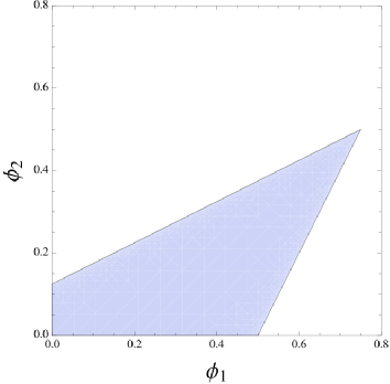
  Figure 1. The allowed region for $\phi$ in case (ii).

  

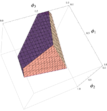
  Figure 2. The allowed region for $\phi$ in case (iii).

  The gradient of the action of a minimizer with respect to $\phi$ is given by

  $$\nabla_{(\phi_{1},\phi_{2})}{\mathcal{S}}_{\mathfrak{I}}[\rho,\phi]=\frac{4}{3}\begin{pmatrix}1+\phi_{2}-2\phi_{1}\\ 1+\phi_{1}-2\phi_{2}\end{pmatrix}\geq\begin{pmatrix}0\\ 1\end{pmatrix}\,,$$

  where the last inequality is meant to hold separately for each of the two components. Thus the minimum of the action in the allowed $\phi$-region lies on the line $\{\phi_{2}=0\}$, and consequently at $(\phi_{1},\phi_{2})=(0,0)$. We thus obtain the following estimate for the action of a minimizer,

  $${\mathcal{S}}_{\mathfrak{I}}[\rho,\phi]=-\frac{4}{3}(1-\phi_{1}-\phi_{2}+\phi_{1}^{2}+\phi_{2}^{2}-\phi_{1}\phi_{2})\geq-\frac{4}{3}\,.$$

• Assume that $(\rho,\phi)\in\mathfrak{S}_{\mathfrak{I}}(\rho_{0})$ is such that $\operatorname{supp}(\rho)=\{1,2,3\}$. Then the EL equation (2.4)reads

  $$\rho_{1}+\frac{1}{2}\rho_{2}+\phi_{1}-1 =0$$

  $$\rho_{2}+\frac{1}{2}\rho_{1}+\phi_{2}-1 =0$$

  $$\rho_{3}+\frac{1}{2}\rho_{2}+\phi_{3}-1 =0\,.$$

  Solving for $\rho$, we obtain

  $$\rho_{1} =1+\phi_{2}-\frac{3}{2}\phi_{1}-\frac{1}{2}\phi_{3}$$

  $$\rho_{2} =\phi_{1}+\phi_{3}-2\phi_{2}$$

  $$\rho_{3} =1+\phi_{2}-\frac{3}{2}\phi_{3}-\frac{1}{2}\phi_{1}\,,$$

  where $\phi\in{\mathbb{B}}^{+}({\mathfrak{I}})$ must be chosen such that the constraints $\rho_{1},\rho_{3}\geq 0$ and $\rho_{2}\geq\frac{1}{2}$ hold. The allowed region for $\phi$ is a compact convex simplicial subset of $(\mathbb{R}^{+})^{3}$, which is plotted in Figure 2. The constraint $\rho_{2}\geq\frac{1}{2}$ implies that

  $$\phi_{1}+\phi_{3}\geq\frac{1}{2}\,.$$ (5.2)

  Therefore, the volume of a minimizer can be estimated by

  $$\rho({\mathfrak{I}})=2-\phi_{1}-\phi_{3}\leq\frac{3}{2}\,,$$

  and the maximal volume is attained along the line $\{\phi_{2}=0\>,\>\phi_{1}+\phi_{3}=\frac{1}{2}\}$. The gradient of the action of a minimizer with respect to $\phi$ is given by

  $$\nabla_{(\phi_{1},\phi_{2},\phi_{3})}{\mathcal{S}}_{\mathfrak{I}}[\rho,\phi]=\begin{pmatrix}2+2\phi_{2}-3\phi_{1}-\phi_{3}\\ 2(\phi_{1}+\phi_{3})-4\phi_{2}\\ 2+2\phi_{2}-3\phi_{3}-\phi_{1}\end{pmatrix}\geq\begin{pmatrix}0\\ 1\\ 0\end{pmatrix}\,,$$ (5.3)

  (where the last inequality is again meant componentwise). Thus the minimum of the action in the allowed $\phi$-region lies in the plane $\{\phi_{2}=0\}$. Setting $\phi_{2}=0$ and $\phi_{1}+\phi_{3}>\frac{1}{2}$, either the first or the third component in (5.3) is strictly positive. Therefore, the constraint (5.2) implies that the minimum of the action lies on the line $\{\phi_{2}=0\>,\>\phi_{1}+\phi_{3}=\frac{1}{2}\}$. This one-dimensional problem can be solved easily, yielding that the minimal action is attained at the points $\phi=(\frac{1}{2},0,0)$ and $\phi=(0,0,\frac{1}{2})$. Hence the action of a minimizer can be estimated by

  $${\mathcal{S}}_{\mathfrak{I}}[\rho,\phi]=2-2(\phi_{1}+\phi_{3})(1+\phi_{2})+\phi_{1}\phi_{3}+\frac{3}{2}(\phi_{1}^{2}+\phi_{3}^{2})+2\phi_{2}^{2}\geq-\frac{11}{8}\,.$$

Combining the above cases (i), (ii), and (iii), we see the following: The optimization problem (A) has the two distinct solutions

$$\rho=\Big{(}\frac{1}{4},\frac{1}{2},\frac{3}{4}\Big{)}\;,\;\phi=\Big{(}\frac{1}{2},0,0\Big{)}\qquad\text{and}\qquad\rho=\Big{(}\frac{3}{4},\frac{1}{2},\frac{1}{4}\Big{)}\;,\;\phi=\Big{(}0,0,\frac{1}{2}\Big{)}\,.$$ (5.4)

The optimization problem (C) has a one-parameter family of solutions

$$\rho_{\tau}=\Big{(}\frac{3}{4}-\tau,\frac{1}{2},\frac{1}{4}+\tau\Big{)}\;,\;\phi_{\tau}=\Big{(}\tau,0,\frac{1}{2}-\tau\Big{)}\qquad\text{with }\tau\in\Big{[}0,\frac{1}{2}\Big{]}\,.$$ (5.5)

Hence, neither the problem (A) nor (C) has a unique solution on the definite set ${\mathfrak{I}}$. Also observe that the two distinct solutions in (5.4) both have minimal action as well as maximal volume.

On the other hand, the optimization problem (D), which maximizes the action in the class of solutions of maximal volume, yields a unique measure $\rho$ according to Theorem 4.14. This solution is obtained by maximizing the action ${\mathcal{S}}_{\mathfrak{I}}[\rho_{\tau},\phi_{\tau}]$ with $(\rho_{\tau},\phi_{\tau})$ given by (5.5),

$$\rho=\Big{(}\frac{1}{2},\frac{1}{2},\frac{1}{2}\Big{)}\quad\text{and}\quad\phi=\Big{(}\frac{1}{4},0,\frac{1}{4}\Big{)}\,.$$ (5.6)

In order to see that the solutions of the optimization problem (B) are also not unique in general, one can add one more point to ${\mathfrak{I}}$, which is space-like separated from all the other points. Thus $\tilde{{\mathfrak{I}}}=\{{\mathfrak{I}},4\}$, and the Lagrangian is represented by the matrix

$$\tilde{{\mathcal{L}}}=\begin{pmatrix}{\mathcal{L}}&0\\ 0&1\end{pmatrix}\,,$$

where ${\mathcal{L}}$ is the matrix in (5.1). The initial data $\tilde{\rho}_{0}=(0,\frac{1}{2},0,0)$ is admissible, and its domain of dependence is $\tilde{{\mathfrak{I}}}$. Any solution of the initial value problem in $\tilde{{\mathfrak{I}}}$ is of the form

$$\tilde{\rho}=(\rho,1-\phi_{4})\quad\text{and}\quad\tilde{\phi}=(\phi,\phi_{4})\,,$$ (5.7)

where $(\rho,\phi)$ is a solution of the initial value problem in ${\mathfrak{I}}$ and $\phi_{4}\in[0,1]$. From the EL equations in the cases (i), (ii) and (iii), it follows that $\max_{\operatorname{supp}(\rho)}\phi\geq\frac{1}{4}$, and hence $\max_{\operatorname{supp}(\tilde{\rho})}\tilde{\phi}\geq\frac{1}{4}$. Thus there is a one-parameter family of solutions of the optimization problem (B) on the definite set $\tilde{{\mathfrak{I}}}$, obtained by taking $(\rho,\phi)$ from (5.6) and choosing $\phi_{4}\in[0,\frac{1}{4}]$ in (5.7).

Acknowledgments: We are grateful to Johannes Kleiner for helpful comments on the manuscript. A.G. would like to thank the German Academic Exchange Service (DAAD) who supported this work by a fellowship within its postdoc program. He is also grateful to the Department of Mathematics at Harvard University for its hospitality while working on the manuscript.

References

- [1] L. Ambrosio and P. Tilli, Topics on Analysis in Metric Spaces, Oxford Lecture Series in Mathematics and its Applications, vol. 25, Oxford University Press, Oxford, 2004.
- [2] Y. Bernard and F. Finster, On the structure of minimizers of causal variational principles in the non-compact and equivariant settings, arXiv:1205.0403 [math-ph], Adv. Calc. Var. 7 (2014), no. 1, 27–57.
- [3] F. Finster, Causal variational principles on measure spaces, arXiv:0811.2666 [math-ph], J. Reine Angew. Math. 646 (2010), 141–194.
- [4] F. Finster and A. Grotz, A Lorentzian quantum geometry, arXiv:1107.2026 [math-ph], Adv. Theor. Math. Phys. 16 (2012), no. 4, 1197–1290.
- [5] F. Finster, A. Grotz, and D. Schiefeneder, Causal fermion systems: A quantum space-time emerging from an action principle, arXiv:1102.2585 [math-ph], Quantum Field Theory and Gravity (F. Finster, O. Müller, M. Nardmann, J. Tolksdorf, and E. Zeidler, eds.), Birkhäuser Verlag, Basel, 2012, pp. 157–182.
- [6] F. Finster and D. Schiefeneder, On the support of minimizers of causal variational principles, arXiv:1012.1589 [math-ph], Arch. Ration. Mech. Anal. 210 (2013), no. 2, 321–364.
- [7] M. Reed and B. Simon, Methods of Modern Mathematical Physics. I, functional analysis, second ed., Academic Press Inc., New York, 1980.