Majorana Fermions in superconducting wires: effects of long-range hopping, broken time-reversal symmetry and potential landscapes

Abstract

We present a comprehensive study of two of the most experimentally relevant extensions of Kitaev’s spinless model of a 1D $p$-wave superconductor: those involving (i) longer range hopping and superconductivity and (ii) inhomogeneous potentials. We commence with a pedagogical review of the spinless model and, as a means of characterizing topological phases exhibited by the systems studied here, we introduce bulk topological invariants as well as those derived from an explicit consideration of boundary modes. In time-reversal invariant systems, we find that the longer range hopping leads to topological phases characterized by multiple Majorana modes. In particular, we investigate a spin model, which respects a duality and maps to a fermionic model with multiple Majorana modes; we highlight the connection between these topological phases and the broken symmetry phases in the original spin model. In the presence of time-reversal symmetry breaking terms, we show that the topological phase diagram is characterized by an extended gapless regime. For the case of inhomogeneous potentials, we explore phase diagrams of periodic, quasiperiodic, and disordered systems. We present a detailed mapping between normal state localization properties of such systems and the topological phases of the corresponding superconducting systems. This powerful tool allows us to leverage the analyses of Hofstadter’s butterfly and the vast literature on Anderson localization to the question of Majorana modes in superconducting quasiperiodic and disordered systems, respectively. We briefly touch upon the synergistic effects that can be expected in cases where long-range hopping and disorder are both present.

I Introduction

The recent explosion of studies concerning Majorana fermions in solid state systems has brought the one-dimensional spinless $p$-wave paired superconducting wire into the limelight. As the prototype for hosting topological phases characterized by bound Majorana states at the ends of the wire, this superconducting system has been theoretically studied from a variety of angles kitaev1 ; beenakker ; lutchyn1 ; oreg ; fidkowski2 ; potter ; fulga ; stanescu1 ; tewari ; gibertini ; lim ; tezuka ; egger ; ganga ; sela ; lobos ; lutchyn2 ; cook ; pedrocchi ; sticlet ; jose ; klinovaja ; alicea ; stanescu2 ; halfmetal ; shivamoggi ; adagideli ; sau ; akhmerov ; degottardi ; ladder ; niu ; period ; lang ; brouwer2 ; brouwer3 ; vish and has formed the basis for several experimental realizations kouwenhoven ; deng ; rokhinson ; das . While these analyses have led to revisiting several theoretical aspects investigated in the past decade, such as topological features and symmetry classification of the system, localization properties in the presence of disorder, and physics in the presence of multiple channels, the prospect of experimental realization has instigated new exploration of physical realizations. A number of studies have focused on novel materials and geometries, as well as subjecting the system to controlled external potentials. Additionally, new means of detecting Majorana modes and signatures of related non-Abelian statistics have been proposed, as well as on applications, such as schemes for topological quantum computation in these systems tjunction ; topqubit .

Here, contributing to this vast literature, we present a comprehensive study of the superconducting wire subject to various experimentally relevant modifications of Kitaev’s original model. By exploring several variants of the coupling/hopping amplitudes and spatially varying electronic potentials, we build on and unify previously studied features of similar models. We investigate physics stemming from long-range hopping wherein conduction electrons in a lattice version of the wire can hop across several sites. In systems obeying time-reversal symmetry, we illustrate how such hopping may give rise to multiple end Majorana fermions. We perform an involved study of the wire in the presence of various potential landscapes, in particular, periodic potentials, quasiperiodic potentials and disorder. Finally, we briefly describe some of the richness associated with systems exhibiting both long-range hopping and inhomogeneous potentials. Our goal here is to present several new results of experimental relevance as well as to gather foundational information that is scattered in the literature, recasting some of it in simpler language and providing the non-expert a pedagogical, self-contained exposition leading up to the results.

We begin with a review of the lattice version of the one-dimensional spinless $p$-wave superconducting fermionic system, namely the Kitaev chain, and focus on its Majorana mode properties. Specifically, we consider the phase diagram and topological features of the system by virtue of the presence of Majorana end modes in some regions of parameter space (topological phases) versus their absence in others (non-topological phase). We develop the formalism for several alternate topological invariants that are useful in different circumstances. The relevant topological invariants can either be derived from bulk properties for a homogeneous system with periodic boundary conditions or boundary properties in long finite-sized wires which pinpoint the existence of end modes; the latter was developed in our previous work in Ref. ladder within a transfer matrix formalism and is easy to apply to a range of situations. This connection provides an elementary illustration of the so-called bulk-boundary correspondence hasan ; qi . The topological invariants (TIs) are either $\mathbb{Z}_{2}$ in nature, detecting odd versus even number of Majorana end modes (and associated $\mathbb{Z}_{2}$ bulk physics), or $\mathbb{Z}$, detecting the presence of multiple, independent Majorana end modes (and associated winding numbers in the bulk), depending on whether time-reversal symmetry (TRS) is obeyed hasan ; qi ; teo . It has been long known that the superconducting system can be mapped to a spin chain, the topological phase being associated with an Ising ferromagnet and the non-topological phase with a paramagnet kitaev1 ; niu ; ladder ; we recapitulate this mapping.

Detailed studies involving symmetry classifications of superconductors have identified the one at hand as having a topological invariant that lies in $\mathbb{Z}$ when time-reversal symmetry is preserved (class BDI). Here, we show that long-range hopping explicitly brings out this $\mathbb{Z}$ character fidkowski1 . Depending on the strength of the hopping terms, the system can exhibit a slew of phases characterized by the presence of multiple, robust, independent Majorana end modes. In terms of bulk properties, these phases are characterized by winding numbers having different integer values. While in terms of lattice connectivity, the basic structure of these Majorana modes is the same as previously discussed modes in multichannel wires fidkowski1 ; potter ; law , our construction explicitly discusses the physics of long-range hopping and can be realized within a single-channel system.

As a specific instance of a long-range hopping, we present a model having second nearest-neighbor hopping that also displays interesting physics in terms of spin variables. The model exhibits four distinct phases, three of which also have analogs in the Kitaev chain, and the fourth phase, being the novel one, supports two independent Majorana modes at each end of a superconducting wire. In the spin language, the model has cubic terms and an elegant duality map between one set of spin variables and another. The four phases correspond to long-range ordering of different spin components in the two sets of spin variables. The models shows a rich phase diagram highlighted by the multiple-Majorana phase in the fermion language and by ordering involving duality maps in the spin language.

The symmetry classification scheme has shown that in the absence of time-reversal symmetry, the topological invariant associated with the system lies in $\mathbb{Z}_{2}$ (class D) hasan ; qi ; teo ; altland ; brouwer1 ; gruzberg ; fidkowski1 . Here, by explicitly describing the system in terms of Majorana fermion degrees of freedom, we discuss the manner in which the $\mathbb{Z}$ form of the invariant for time-reversal symmetric systems gets reduced to $\mathbb{Z}_{2}$ once symmetry breaking terms are introduced. We consider the effect of such terms on the Kitaev chain phase diagram, in particular, the presence of a complex phase in the superconducting order parameter. We show that such a phase gives rise to an unusual extended, gapless, capsule-like region that lies between the gapped topological and non-topological regions.

The presence of spatially varying potentials too causes dramatic changes to the topological phase diagram of the superconducting wire. Expanding on our results of Ref. degottardi , we develop our transfer matrix formalism and show that the manner in which Majorana end mode wave functions decay into the bulk of the system can be connected to localization properties of a normal system (vanishing superconducting gap) described by the same potential landscape (similar methods have been employed in adagideli ; beenakker ; sau ). Moreover, for a common class of potentials, we show that there exists a mapping between the phase boundary for fixed gap strength and its inverse. Armed with the transfer matrix tool, we analyze the effect of several different potential landscapes. As the simplest case, periodic potentials significantly affect the topological phase boundary, providing a knob to control the extent of the topological regime. For quasiperiodic potentials, the map to normal systems provides significant insight and reveals that the topological phase diagram mirrors fractal-like structures, like the Hofstadter butterfly, that naturally emerge in normal systems possessing quasiperiodicity.

Finally, for disordered potentials, the mapping to normal state properties is powerful in that it allows us to leverage the extensive literature on Anderson localization in normal systems to identify the topological phase diagram for the disordered superconductor. We consider a variety of potentials, including uniformly- and Lorentzian-distributed disorder. All examples show that the topological phase continues to occupy a significant region of the phase diagram in the presence of disorder. One of our findings is a ubiquitous singularity in the phase boundary at the random-field transverse Ising critical point. While we present a fairly extensive set of phase diagrams and analyses of Majorana physics, our main contribution, the map to normal systems, is much more far-reaching in extent.

Our presentation is as follows. In Sec. I, we introduce our framework in the context of a review of the Kitaev chain. In Sec. II, we describe the generic long-range hopping model and Sec. III the specific instance of the four-phase model. In Sec. IV, we discuss the effect of time-reversal symmetry breaking. In Sec. V, in the context of spatially varying potentials, we further develop the transfer matrix technique introduced in Sec. I and apply the methods to the case of periodic and quasiperiodic potentials. We analyze disordered potentials in Sec. VI and conclude in Sec. VII.

II Review: Topological Aspects of a $p$-wave Superconducting Wire

We review the salient features of a single-channel $p$-wave paired superconducting wire within the context of the broadly-used 1D tight-binding system of spinless electrons pioneered by Kitaev kitaev1 (referred to as Kitaev chain). We approach this simple and well-studied system from various angles as a preparation for the new material in subsequent sections. We discuss the phase diagram of the Kitaev chain in terms of its topological properties characterized by the presence or absence of zero energy Majorana modes at the ends of a long and open chain. To establish these topological properties, we consider two symmetry classes, one respecting time-reversal invariance and the other breaking it. To analyze these classes, we present various topological invariants, some exploiting bulk features of the Hamiltonian in momentum space and others explicitly counting the number of zero energy modes at the ends of an open chain. Finally, we review the Jordan-Wigner transformation lieb which maps the fermionic system to a spin-1/2 chain.

II.1 Kitaev Chain: Model, Dispersion and Phases

In this lattice description of the single-channel $p$-wave superconductor, electrons experience a nearest-neighbor hopping amplitude $w$, a superconducting gap function for pairing between neighboring sites, $\Delta$, and an on-site chemical potential $\mu$; in this section, we will assume that all these parameters are real. For a finite and open wire with $\mathcal{N}$ sites, the Hamiltonian takes the form

$$H=\sum_{n=1}^{\mathcal{N}-1}\Big{[}-w\left(f_{n}^{\dagger}f_{n+1}+f_{n+1}^{\dagger}f_{n}\right)+\Delta\Big{(}f_{n}f_{n+1}+f_{n+1}^{\dagger}f_{n}^{\dagger}\ \Big{)}\Big{]}~{}-~{}\sum_{n=1}^{\mathcal{N}}\mu\left(f_{n}^{\dagger}f_{n}-1/2\right),$$ (1)

where the operators $f_{n}$ satisfy the usual anticommutation relations $\{f_{m},f_{n}\}=0$ and $\{f_{m},f_{n}^{\dagger}\}=\delta_{mn}$. We can assume that $w>0$; if $w<0$, we can change its sign by the unitary transformation $f_{n}\to(-1)^{n}f_{n}$. (Throughout this paper we will set both $\hbar$ and the lattice spacing equal to unity). It is important to note that Majorana end modes can only appear if the superconducting order parameter $\Delta\neq 0$. This is because Majorana modes do not have a definite fermion number, while the Hamiltonian commutes with the total fermion number, $\sum_{n=1}^{\mathcal{N}}f_{n}^{\dagger}f_{n}$, if $\Delta=0$

Towards exploring the Majorana mode structure of the wire, we can decompose the electron operator in terms of real (Majorana) operators $a$ and $b$ as

$$f_{n}~{}=~{}\frac{1}{2}~{}(a_{n}+ib_{n}),~{}~{}~{}~{}~{}~{}f_{n}^{\dagger}~{}=~{}\frac{1}{2}~{}(a_{n}-ib_{n}).$$ (2)

The operators $a_{n}$ and $b_{n}$ are Hermitian and satisfy $\{a_{m},a_{n}\}=\{b_{m},b_{n}\}=2\delta_{mn}$ and $\{a_{m},b_{n}\}=0$. Then Eq. (1) can be re-written as

$$H = -\frac{i}{2}~{}\sum_{n=1}^{\mathcal{N}-1}\Big{[}(w-\Delta)a_{n}b_{n+1}+(w+\Delta)a_{n+1}b_{n}\Bigl{]}~{}-\frac{i}{2}~{}\sum_{n=1}^{\mathcal{N}}\mu a_{n}b_{n},$$ (3)

To study the bulk features of the system, we consider a long wire having periodic boundary conditions (so that the first summation in Eq. (1) goes from $n=1$ to $\mathcal{N}$). Then the momentum $k$ is a good quantum number and it goes from $-\pi$ to $\pi$ in steps of $2\pi/\mathcal{N}$. Defining the Fourier transform $f_{k}~{}=~{}\frac{1}{\sqrt{\mathcal{N}}}~{}\sum_{n=1}^{\mathcal{N}}~{}f_{n}~{}e^{ikn}$, Eq. (1) can be re-written in momentum space as

$$H = \sum_{0<k<\pi}~{}\left(\begin{array}[]{cc}f_{k}^{\dagger}&f_{-k}\end{array}\right)~{}h_{k}~{}\left(\begin{array}[]{c}f_{k}\\ f_{-k}^{\dagger}\end{array}\right),$$ (7)

$$h_{k} = -(2w\cos k+\mu)~{}s^{z}~{}+~{}2\Delta\sin k~{}s^{y},$$ (8)

where the $s^{a}$ are Pauli matrices denoting pseudo-spin degrees of freedom formed by the fermion particle-hole subspace. The dispersion relation follows from this and is given by

$$E_{k}~{}=~{}\pm~{}\sqrt{(2w\cos k+\mu)^{2}~{}+~{}4\Delta^{2}\sin^{2}k}.$$ (9)

The energy vanishes at certain values of $k$; these are given by lines in the two-dimensional space of the parameters $\mu/w$ and $\Delta/w$. These gapless lines correspond to phase transition lines which separate different phases. The phase diagram consists of three lines demarcating phases I, II and III, as shown in the top left diagram in Fig. 4. On the vertical red lines lying along $\mu/w=\pm 2$, the energy vanishes at $k=\pi$ and zero respectively, while on the horizontal blue line extending from $\mu/w=-2$ to $2$ at $\Delta/w=0$, the energy vanishes at $k=\cos^{-1}(-\mu/(2w))$.

Phase Diagram– To obtain insight into the nature of the phases, we can consider some extreme limits. As shown in Fig. 1 (a), for $\Delta=w=0$, $\mu\neq 0$, which lies in phase III of the phase diagram, we see in terms of the Majorana mode Hamiltonian of Eq. (3) that each Majorana mode $a_{n}$ on a given site is bound to its partner $b_{n}$ with strength $\mu$, leaving no unbound modes. For $\Delta=w\neq 0$, $\mu=0$, lying in phase I, the only existing bonds connect $a_{n}$ to its neighbor $b_{n+1}$ (Fig. 1 (b)), leaving a free $a/b$-Majorana mode at the right/left end of a finite sized system (Fig. 1 (c)). For $\Delta=-w\neq 0$, $\mu=0$, lying in phase II, the roles of $a$ and $b$ modes become interchanged. As shown using topological arguments in the next section, the presence/absence of these end modes is robust in that deviations from these extreme limits in parameter space does not change these features unless a phase boundary associated with a vanishing gap is crossed.

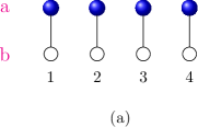
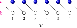
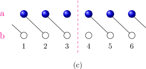
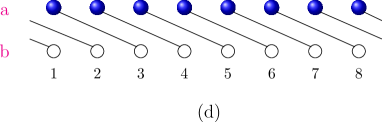
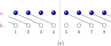
Figure 1: Pictures of a fermionic chain showing the couplings between Majorana operators $a_{n}$ and $b_{n}$ at different sites when only one kind of interaction, $a_{m}b_{n}$, is present in the Hamiltonians in Eqs. (3) and (20). Panels (a), (b) and (d) respectively show couplings of the form $a_{n}b_{n}$, $a_{n}b_{n+1}$ (Eq. (3)) and a longer range interaction $a_{n}b_{n+2}$ (Eq. (20)) in the middle of a long chain. Panels (c) and (e) show couplings of the form $a_{n}b_{n+1}$ and $a_{n}b_{n+2}$ for a chain which has been cut into two, thus giving two open chains. Panel (c) has a Majorana mode $a_{3}$ at the right end and a mode $b_{4}$ at the left end of an open chain. Panel (e) has two Majorana modes $a_{3}$ and $a_{4}$ at the right end of an open chain and two modes $b_{5}$ and $b_{6}$ at the left end of an open chain. (Panel (a) would not have any Majorana end modes for a chain cut into two).

II.2 Topological Invariants (TIs), Transfer Matrix Approach and Majorana Modes

The topological properties of the superconducting wire described above can be captured in a variety of ways, all involving global features of the system characterized by TIs. There are several TIs developed in the literature; some are a type of generalized winding number (for instance, the celebrated TKKN invariant of the integer quantum Hall effect thouless ) or are based on a Pfaffian, as in kitaev1 . Building on previous work ladder ; degottardi , we introduce complementary ‘boundary invariants’, i.e. TIs which are derived from an explicit counting of the number of edge Majorana states. It should be emphasized that although the bulk and boundary invariants are derived in different ways, they all share two crucial characteristics: (1) they are restricted to integer values and (2) small deformations of the Hamiltonian which do not close a bulk gap cannot change their values. Furthermore, they enumerate the number of edge Majorana modes. The different forms will be used in subsequent sections based on convenience and the aspects studied.

Symmetry Classes– In this paper we will encounter both $\mathbb{Z}$ and $\mathbb{Z}_{2}$ TIs (which we explain below). These types indicate the level of topological protection enjoyed by a topological insulator or superconductor. An extensive classification of topological insulators and superconductors has been developed, and the type of TI can be determined from the class which the Hamiltonian falls into hasan ; qi ; teo . The class depends on a number of factors, such as whether the particles are bosons or fermions and whether the Hamiltonian has spin rotation symmetry (if the particles have a non-zero spin), particle-hole symmetry or TRS. The different symmetry classes have been enumerated and there is extensive discussion in the literature altland ; motrunich ; brouwer1 ; gruzberg ; fidkowski1 . Relevant to this work are the classes:

Class D – This class is appropriate for describing spinless electrons exhibiting $p$-wave pairing but for which time-reversal symmetry is broken altland ; brouwer1 ; gruzberg ; fidkowski1 . This class exhibits $\mathbb{Z}_{2}$ topological protection (in 1D) indicating that the parity of the number of Majorana modes is protected kitaev1 ; hasan ; qi ; teo .

Class BDI – This class also describes spinless electrons exhibiting $p$-wave pairing, with the additional restriction that time-reversal symmetry is obeyed. This class is associated with a $\mathbb{Z}$ TI in 1D, indicating that the number of Majorana modes itself is topologically protected fidkowski1 .

As is seen here, a general feature of the ‘periodic table of topological insulators’ is that the level of topological protection is generally greater as the symmetry constraints on the Hamiltonian become more restrictive hasan ; qi ; teo ; fidkowski1 .

II.2.1 Bulk Invariants

Depending on the time-reversal properties of the Hamiltonian $h_{k}$, two different invariants can be defined. (Although Eq. (8) defines $h_{k}$ only for $0\leq k\leq\pi$, it will now be convenient to use the same expression for $h_{k}$ for the entire range $0\leq k\leq 2\pi$). In Eq. (8), we see that $h_{k}$ is of the form $h_{k}=a_{3k}s^{z}+a_{2k}s^{y}$, which maps to the vector $\vec{V}_{k}=a_{3k}\hat{z}+a_{2k}\hat{y}$ in the $z-y$ plane. The form is general to this class of systems which have TRS, i.e., when $h^{*}_{-k}=h_{k}$ for all $k$. Our first bulk invariant $W$, as introduced in Refs. niu ; tong , is then the winding number associated with the angle $\phi_{k}=\tan^{-1}(a_{2k}/a_{3k})$ made by the vector $\vec{V}_{k}$ with respect to the $\hat{z}$ axis upon traversing the Brillouin zone, i.e.,

$$W~{}=~{}\int_{0}^{2\pi}~{}\frac{dk}{2\pi}~{}\frac{d\phi_{k}}{dk}.$$ (10)

This object can take any integer value and is a TI, namely, it does not change under small changes in $h_{k}$ unless $h_{k}$ happens to pass through zero for some value of $k$; in the latter case, the winding number becomes ill-defined and the energy $E_{k}=0$ which means that the bulk gap closes at that value of $k$. As will be explicitly discussed for the case of long-range hopping, we thus have a $\mathbb{Z}$-valued invariant, as expected from the general classification discussed above. It is straightforward to determine the relationship between $W$ and the number of edge modes $N_{a}$ and $N_{b}$ of $a$ and $b$ type (respectively) of Majorana modes at the left-hand end of an open chain, and confirm that $W=N_{b}-N_{a}$. Note that taking $\Delta\rightarrow-\Delta$ reverses the winding of $\vec{V}_{k}$ and thus $W$, which is consistent with this transformation interchanging $a$ and $b$ Majoranas (see Sec. II.1).

In the absence of TRS, i.e., if $h^{*}_{-k}\neq h_{k}$ for some $k$, as seen in later sections, $h_{k}$ generally has four components, $h_{k}=a_{0k}I+a_{1k}s^{x}+a_{2k}s^{y}+a_{3k}s^{z}$, and it is not possible to define a winding number for the corresponding vector in four dimensions. On the other hand, for momentum values $k=0$ and $\pi$, $h_{k}$ has only one component, namely, $h_{0}=h(0)s^{z}$ and $h_{\pi}=h(\pi)s^{z}$. As seen in Eq. (8), this is naturally true also in the case with TRS. Under the stringent assumption that the system is fully gapped (i.e., gapped for all values of $k$), one can define a $\mathbb{Z}_{2}$-valued TI:

$$\nu_{bulk}=\mbox{sgn}\left(h(0)h(\pi)\right).$$ (11)

This invariant can take the values $-1$ or $1$ and is topological in that its value cannot change unless either $h(0)$ or $h(\pi)$ crosses zero in which case the energy $E_{0}$ or $E_{\pi}$ vanishes. We will see that $\nu_{bulk}$ is equal to the parity of the number of Majorana modes at the end of the system.

The fact that systems which break TRS have a symmetry only at the level $\mathbb{Z}_{2}$ may also be seen another way. As seen above, sending $\Delta\rightarrow-\Delta$ takes $W\rightarrow-W$. This process can be carried out for class D without closing a gap since we can take $\Delta=\Delta_{0}e^{i\varphi}$ and take $\varphi$ from $0\rightarrow\pi$. However, for class BDI, $\Delta$ is constrained to be real and the only way to take $\Delta\rightarrow-\Delta$ is to pass through zero, which closes a gap fidkowski1 .

II.2.2 Boundary Invariants: Transfer Matrix Approach

We now outline the transfer matrix approach detailed in our previous work, Ref. ladder , for identifying the Majorana modes structure at the end of a wire. It will become apparent that the transfer matrix explicitly gives us $N_{a}$ and $N_{b}$ (as defined in the previous section, $N_{a,b}$ is the number of $a$- and $b$-type Majorana modes at the left-hand side of the system, respectively). We also note that finding $N_{a}$ and $N_{b}$ from the transfer matrix will only involve finding the eigenvalues of a matrix; this is numerically easier than calculating than $W$ which involves doing an integral over the momentum $k$.

The transfer matrix can be obtained from the Heisenberg equations of motion for the Majorana operators in Eq. (3):

$$i\frac{da_{n}}{dt} = -~{}[H,a_{n}]~{}=~{}-i(w+\Delta)b_{n+1}~{}-~{}i(w-\Delta)b_{n-1}~{}-~{}i\mu b_{n},$$

$$i\frac{db_{n}}{dt} = -~{}[H,b_{n}]~{}=~{}i(w+\Delta)a_{n-1}~{}+~{}i(w-\Delta)a_{n+1}~{}+~{}i\mu a_{n}.$$ (12)

Assuming that these operators depend on time as $a_{n}=\alpha_{n}e^{-iEt}$ and $b_{n}=\beta_{n}e^{-iEt}$, we find the values of the energy $E$ for which the above equations have solutions. The solutions in the bulk have the same dispersion as the one given in Eq. (9); in particular, the energies differ from zero by a finite gap except on the phase boundaries. In addition to these bulk modes, in the topological phases there are end modes which lie at zero energy for long chains and are therefore separated by a gap from the bulk modes. (For short chains, modes at the two ends can hybridize and lift their degeneracy away from zero.) For $E=0$, Eqs. (12) take the form

$$(w+\Delta)\alpha_{n+1}~{}+~{}(w-\Delta)\alpha_{n-1}~{}+~{}\mu\alpha_{n} = 0,$$

$$(w+\Delta)\beta_{n-1}~{}+~{}(w-\Delta)\beta_{n+1}~{}+~{}\mu\beta_{n} = 0.$$ (13)

These equations can be represented in the transfer matrix form

$$\left(\begin{array}[]{c}\alpha_{n+1}\\ \alpha_{n}\end{array}\right)=~{}A_{n}\left(\begin{array}[]{c}\alpha_{n}\\ \alpha_{n-1}\end{array}\right),~{}~{}\mbox{where}~{}~{}A_{n}=\left(\begin{array}[]{cc}-\frac{\mu}{\Delta+w}&\frac{\Delta-w}{\Delta+w}\\ 1&0\end{array}\right).$$ (14)

Since the $A_{n}$ may be taken as functions of $\mu/w$ and $\Delta/w$, we set $w=1$. A similar expression holds for the transfer matrix $B_{n}$ for the $\beta_{n}$. (In a later section, we will consider models where the chemical potential $\mu_{n}$ and therefore $A_{n}$ and $B_{n}$ vary with $n$).

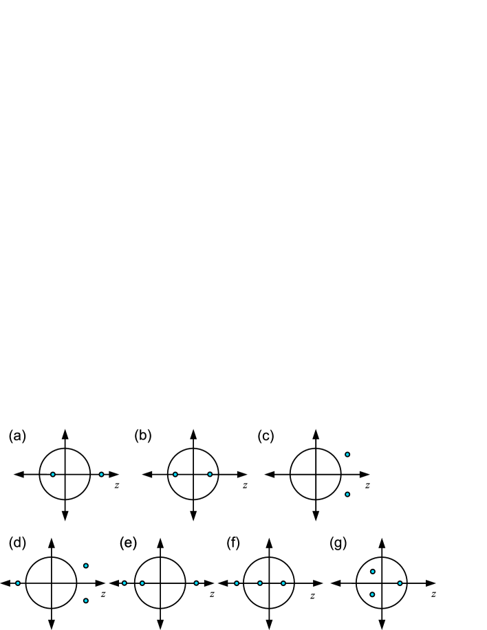
Figure 2: Panels (a-c): Possible locations of the eigenvalues of a $2\times 2$ transfer matrix for Majorana mode $a$ as discussed in Sec. II B. Only one eigenvalue may lie inside the unit circle as in (a), or both eigenvalues may lie inside the unit circle as in (b), or both may lie outside the unit circle as in (c). Panel (d-g): Possible locations of the eigenvalues of a $3\times 3$ transfer matrix for Majorana mode $b$ as analyzed in Sec. V A. As discussed in the text, the number and type of Majorana modes at each end of a long chain is governed by the number of eigenvalues inside the unit circle; cases (a) and (e) give non-topological phases characterized by the absence of end modes, while all the other cases give topological phases with one or more end modes at each end.

The existence of end Majorana modes requires the $\alpha_{n}$ (or $\beta_{n}$) to be normalizable, i.e., $\sum_{n}|\alpha_{n}|^{2}$ (or $\sum_{n}|\beta_{n}|^{2}$) should be finite. The number of eigenvalues of the full transfer matrix $\mathcal{A}\equiv\prod_{n=1}^{\mathcal{N}}A_{n}$ with magnitude less than 1 is denoted by $n_{f}$. The number $n_{f}$ corresponds to the number of roots of the characteristic polynomial for the transfer matrix, $f(z)=\det\left(I-\mathcal{A}z\right)$, that lie within the unit circle. Hence,

$$n_{f}=\frac{1}{2\pi i}\oint_{|z|=1}~{}dz~{}f^{\prime}(z)/f(z),$$ (15)

as was noted in the context of plane wave zero modes in Ref. wen . One can show that the eigenvalues of the full transfer matrix $\mathcal{B}\equiv\prod_{n=1}^{\mathcal{N}}B_{n}$ are inverses of the eigenvalues of $\mathcal{A}$, and therefore the number of eigenvalues of $\mathcal{B}$ with magnitude smaller than 1 is $2-n_{f}$. For $n_{f}=0$ and 2, $\alpha_{n}$ and $\beta_{n}$ are normalizable and therefore the system is topological (with a $\alpha$ mode at one end and a $\beta$ mode at the other end of a long chain), whereas for $n_{f}=1$, $\alpha_{n}$ and $\beta_{n}$ are not normalizable and the system is non-topological.

With $n_{f}$ at hand, we can define a $\mathbb{Z}_{2}$ invariant

$$\nu_{end}~{}=~{}-~{}(-1)^{n_{f}}=-\mbox{sgn}\left(f(1)f(-1)\right),$$ (16)

for which $\nu_{end}=-1$ and $\nu_{end}=1$ reflect an odd versus even number of normalizable end Majorana modes, respectively. For the Kitaev chain of Eq. (1), since there can only be one or zero modes, these values correspond to topological and non-topological phases, respectively. Since the topology of the system depends only on the magnitude of $\Delta$, we take $\Delta$ to be positive; hence $|\det~{}\mathcal{A}|<1$. Then the two eigenvalues of $\mathcal{A}$ obey $|\lambda_{1}\lambda_{2}|<1$. Therefore, for $|\lambda_{1}|<|\lambda_{2}|$, we have $|\lambda_{1}|<1$ and $n_{f}$ is completely determined by the larger eigenvalue $\lambda_{2}$. Thus, we have that $\nu=\mbox{sgn}\left(\ln|\lambda_{2}|\right)$ for $\Delta>0$. We claim that the odd-even Majorana structure denoted by the $\mathbb{Z}_{2}$ invariant $\nu_{end}$ of Eq. (16) matches the form of the bulk invariant $\nu_{bulk}$ of Eq. (11).

Phase Diagram – We can now revisit the Kitaev chain phase diagram in light of these invariants. Considering some special cases, for $\mu=0$ and $\Delta>0$, we find that both eigenvalues of $\mathcal{A}$ have magnitude smaller than 1, so that $n_{f}=2$. Further, we find that there is a zero energy Majorana mode of type $a$ at the left end and of type $b$ at the right end of a long chain. This describes phase I following the discussion after Eq. (9). If $\mu=0$ and $\Delta<0$, both eigenvalues of $\mathcal{A}$ have magnitude larger than 1, so that $n_{f}=0$. We find that there is a zero energy Majorana mode of type $b$ at the left end and of type $a$ at the right end of a long chain. This describes phase II. Finally, let us consider $\Delta=0$ and $|\mu|>2t$. This lies in phase III. We then find that $n_{f}=0$ and that there are no Majorana modes at either end of a long chain. This is summarized in Table I.

Phase	$\nu$	$W$	$n_{f}$	$N_{a}$	$N_{b}$
I	$-1$	$-1$	$2$	$1$	$0$
II	$-1$	$1$	$0$	$0$	$1$
III	$1$	$0$	$1$	$0$	$0$

Table 1: Summary of the topological phases (I and II) and non-topological phase (III) exhibited by the Hamiltonian of Eq. (1) and the different topological invariants. Here $\nu$ refers to both $\nu_{bulk}$ and $\nu_{end}$, consistent with their equivalence.

Note that on the phase transition lines which separate the various phases, the bulk gap closes, i.e., $E_{k}=0$ at certain real values of the momentum $k$. Eqs. (13) and (14) then imply that $A_{n}$ must have an eigenvalue of the form $e^{ik}$ which lies on the unit circle. Thus the eigenvalues of the transfer matrix cross the unit circle as we go across a phase transition line.

The TIs that we have discussed here are related to other invariants which exist in the literature. We refer the reader to Refs. teo ; wen ; ladder .

II.3 Mapping to a Spin-1/2 Chain

The Hamiltonian in Eq. (3) can be mapped to that of a spin-1/2 chain; here we briefly review the mapping and associated physics lieb . We define the Jordan-Wigner (JW) transformation between a spin-1/2 and a spinless fermion at each site $n$ so that the states with $\sigma_{n}^{z}=\pm 1$ correspond to the fermion number $f_{n}^{\dagger}f_{n}=1$ and 0 respectively. The JW transformation takes the form

$$a_{n} = \left(\prod_{i=1}^{n-1}\sigma_{i}^{z}\right)~{}(-1)^{n}~{}\sigma_{n}^{y},~{}~{}~{}~{}~{}~{}b_{n}~{}=~{}\left(\prod_{i=1}^{n-1}\sigma_{i}^{z}\right)~{}(-1)^{n}~{}\sigma_{n}^{x}.$$ (17)

Eq. (3) can then be re-written as

$$H~{}=~{}-~{}\sum_{n=1}^{\mathcal{N}-1}\Big{[}J_{x}\sigma_{n}^{x}\sigma_{n+1}^{x}+J_{y}\sigma_{n}^{y}\sigma_{n+1}^{y}\Bigl{]}~{}-~{}\frac{1}{2}~{}\sum_{n=1}^{\mathcal{N}}~{}h\sigma_{n}^{z},$$ (18)

with

$$J_{x}=\left(w-\Delta\right)/2,\ J_{y}=\left(w+\Delta\right)/2,\ h=\mu.$$ (19)

The Hamiltonian describes a spin chain having nearest-neighbor $xx$ and $yy$ couplings and a magnetic field pointing in the $z$ direction.

In the discussion below Eq. (9), we had stated that there are three phases, I, II and III, depending on the values of the parameters $\mu/w$ and $\Delta/w$. While in the fermionic language the ordering is topological in nature and has no local order, we can see that in the spin language, the corresponding phases are described by ordering of local spin variables. Assuming that $w>0$, let us first consider $\mu=0$. Then the point $\Delta=w$ lies in phase I and corresponds to $J_{x}=0$ and $J_{y}=w>0$. This describes a ferromagnetic Ising model with $yy$ couplings which has long-range order in $\sigma^{y}$. Similarly, $\Delta=-w$ lies in phase II and describes a ferromagnetic Ising model with $xx$ couplings which has long-range order in $\sigma^{x}$. Finally, $\Delta=0$ and $|\mu|\gg 2w$ describes a model with $J_{x}=J_{y}$ and a magnetic field in the $z$ direction whose magnitude is much larger than $J_{x}$. This describes a system with no long-range order in either $\sigma^{x}$ or $\sigma^{y}$. These special points represent the entire phase diagram in that phase III is that of a disordered paramagnet, and phases I and II have Ising ferromagnetic order (along $y$ and $x$, respectively) and are separated by a gapless line ($\Delta=0$, $J_{x}=J_{y}$) describing an $xy$ ordered spin chain in a transverse field.

While the spin chain described above has a venerable history in and of itself, the mapping sets the stage for more complicated spin systems and mappings in the context of topological order, such as with the Kitaev honeycomb model kitaev2 and the Kitaev ladder vish ; ladder . In Sec. IV, we will discuss an interesting generalization of the fermionic model, which has multiple Majorana modes and exhibits a rich phase diagram, that can be elegantly described in terms of spin variables.

III Long-range Hopping and Multiple Majorana End Modes

Here we argue that the presence of longer range hopping that extends beyond the nearest neighbor has the dramatic consequence that in a spinless superconducting wire that preserves TRS, multiple topologically protected Majorana modes can form at the ends of the wire. These modes are stable in that regions in parameter space corresponding to different number of modes are protected by bulk gaps in the energy spectrum and correspond to topologically distinct phases. In the previous analyses of symmetry classes mentioned above, it has been argued in various ways that the TI lies in $\mathbb{Z}$ for the class currently being considered, class BDI. The discussion here in terms of long-range hopping in a single-channel model and of the TIs defined above gives a simple, direct and comprehensive picture for the $\mathbb{Z}$ form by way of multiple Majorana end modes.

Below we introduce the general long-range hopping model and analyze its topological properties based on the presence of multiple Majorana end modes. In the next section, we explore the features of the aforementioned model having four topologically distinct phases and a dual Ising representation in the language of spins.

III.1 Long-range Hopping Model

As a very general case of long-range hopping, we consider a modification to the Kitaev chain of the previous section that takes into account an infinite set of couplings for long-range hopping. Focusing purely on the hopping and pairing, this generalized version of the Majorana Hamiltonian of Eq. (3) for an infinite wire takes the form

$$H~{}=~{}-i\sum_{r=-\infty}^{\infty}~{}\sum_{n=-\infty}^{\infty}~{}J_{r}~{}a_{n}b_{n+r},$$ (20)

where the $J_{r}$ are real parameters. Note that we have chosen to discuss long-range hoppings in a single chain. However, our model is equivalent, for appropriate choices of the $J_{r}$, to a multi-chain system with both interchain and intrachain couplings.

The Hamiltonian in Eq. (20) is invariant under TRS which involves complex conjugating all numbers, taking the time $t\to-t$, changing $a_{n}\to-a_{n}$ and keeping $b_{n}$ unchanged. The transformation of $a_{n}$ is justified by Eq. (17) where we see that complex conjugating reverses the sign of $\sigma_{n}^{y}$ and therefore of $a_{n}$. Note that the square of the time-reversal transformation is equal to $+1$ since it leaves $a_{n}$ and $b_{n}$ unchanged.

In terms of Dirac fermions $f_{n}=(a_{n}+ib_{n})/2$ and $f_{n}^{\dagger}=(a_{n}-ib_{n})/2$, the generalized momentum space version of Eq. (8) momentum space stemming from Eq. (20) takes the form

$$H = \sum_{0<k<\pi}~{}\left(\begin{array}[]{cc}f_{k}^{\dagger}&f_{-k}\end{array}\right)~{}h_{k}~{}\left(\begin{array}[]{c}f_{k}\\ f_{-k}^{\dagger}\end{array}\right),$$ (24)

$$h_{k} = -2\sum_{r=-\infty}^{\infty}~{}[J_{r}\cos(kr)~{}s^{z}~{}+~{}J_{r}\sin(kr)~{}s^{y}],$$ (25)

where the $s^{a}$ are once again Pauli matrices.

Note that the Hamiltonian is time-reversal invariant: $h^{*}_{-k}=h_{k}$. The energy-momentum dispersion follows from Eq. (25),

$$E_{k}~{}=~{}\pm 2\sqrt{\left(\sum_{r}J_{r}\cos(kr)\right)^{2}~{}+~{}\left(\sum_{r}J_{r}\sin(kr)\right)^{2}}.$$ (26)

The phase diagram can, in principle, be found from this expression by demanding that $E_{k}$ should vanish for some value of $k$ lying in the range $[0,\pi]$ or by employing the TIs defined in the previous section. While this is a difficult problem, we will see below that a great deal of insight can be gained by considering situations in which one of the $J_{r}$ is much larger than all the others.

III.2 Multiple Majorana Modes and Topological Phases

To address what phases are exhibited by the model for an infinitely long chain and how many zero energy Majorana modes there are for the ends of a long chain in the different phases, consider a Hamiltonian where one of the $J_{r}$, say $J_{q}$ for some positive integer $q$, is non-zero and positive while all the others are zero fidkowski1 . (From Eq. (20) we see that the ground state is then given by a state in which $ia_{n}b_{n+q}=1$ for each $n$). We show this situation in Fig. 1 (d) for the case of $q=2$. In Fig. 1 (e), we have shown a dotted line which cuts the chain into two; it is clear that the open chain on the right side has $q$ Majorana modes of type $b$ at its left end, while the open chain on the left side has $q$ Majorana modes of type $a$ at its right end. Since we expect the number of Majorana modes and their types to be TIs, this phase will survive for small changes in the values of all the other $J_{r}$. We therefore conclude that the model in Eq. (20) has an infinite number of phases which can be labeled by an integer $q$ which describes the number and types of Majorana modes at the ends of a long chain.

Next, we look at what the $\mathbb{Z}$-valued bulk invariant, $W$, defined in Eq. (10) gives for the Hamiltonian in Eq. (25). As before, we can think of $h_{k}$ as defining a two-dimensional vector. If only one of the couplings $J_{q}$ is non-zero and positive, the vector is given by

$$\vec{V}_{k}~{}=~{}-2~{}[J_{q}~{}\cos(kq)~{}\hat{z}~{}+~{}J_{q}~{}\sin(kq)~{}\hat{y}].$$ (27)

As $k$ goes from $0$ to $2\pi$, this generates a closed curve which encircles the origin of the $z-y$ plane $q$ times in the clockwise direction. Defining $\phi_{k}=\tan^{-1}(V_{y}/V_{z})$ and using Eq. (10), we find that the winding number is equal to $q$ for the configuration given in Eq. (27), i.e., $W=q$. Thus the winding number is also equal to the number of Majorana modes of type $b$ ($a$) at the left (right) end of a long chain. We can now consider what happens if all the $J_{r}$ are allowed to be non-zero; the vector is then given by

$$\vec{V}_{k}~{}=~{}-2\sum_{r}~{}[J_{r}~{}\cos(kr)~{}\hat{z}~{}+~{}J_{r}~{}\sin(kr)~{}\hat{y}].$$ (28)

The winding number is a TI and therefore does not change under small changes in all the $J_{r}$. The system thus continues to remain in the phase $q$ as long as the closed curve does not pass through the origin for any value of $k$. But if the curve passes through the origin for some value of $k$, the energy vanishes at that value of $k$ and the system lies at a quantum critical point separating two phases having different topological values $q$.

Transfer matrix approach with constraint equations – We can also understand the existence of Majorana end modes using the transfer matrix approach. Consider a semi-infinite chain, with sites going from $n=1$ to $\infty$, with a Hamiltonian of the form

$$H~{}=~{}\sum_{n=1}^{\infty}~{}\sum_{m=1}^{q}\left(w_{m}f_{n+m}^{\dagger}f_{n}+\Delta_{m}f_{n+m}^{\dagger}f_{n}^{\dagger}+\mbox{H.c.}\right)~{}-~{}\sum_{n=1}^{\infty}~{}\mu_{n}(f_{n}^{\dagger}f_{n}-1/2),$$ (29)

where $w_{m}$, $\Delta_{m}$ and $\mu_{n}$ are all real, and $q\geq 1$ is an integer. Let us now study the zero energy equations of motion to see if there are Majorana modes localized near $n=1$, i.e., the left end of the chain. To be specific, let us focus on the $a_{n}$ modes. Each site $n\geq q+1$ gives rise to an equation linking $a_{n}$ to all sites from $a_{n-q}$ to $a_{n+q}$; these equations can be described by a $d\times d$ transfer matrix $A$, where $d=2q$. However, for $n=1,2,\cdots,q$, all the sites up to $a_{n-q}$ are not present in the system; hence the corresponding equations are not of the transfer matrix form, but instead provide $q$ constraints on the first $2q$ values of $a_{n}$. Let us now suppose that the parameters $(w_{m},\Delta_{m},\mu_{m})$ are such that the transfer matrix $A$ has $n_{f}$ eigenvalues with magnitude smaller than 1, and the other $d-n_{f}$ eigenvalues have magnitude larger than 1. The eigenvectors corresponding to the first $n_{f}$ eigenvalues are normalizable. However, the presence of $q$ constraints means that there are only $n_{f}-q$ independent and normalizable end modes. Thus, the number of $a$ Majoranas on the left-hand side of the system is

$$N_{a}=n_{f}-q.$$ (30)

If $n_{f}\leq q$, there are no Majorana end modes of type $a$. A similar analysis carried out for the $b_{n}$ modes indeed shows that there are an equal number of $b$ Majoranas localized to the opposite end of the system. Finally, we also note that this argument implies that $a$ and $b$ type Majoranas can never occur on the same side of the system. Such a state is incompatible with TRS. As illustrations, models of the form given in Eq. (29) with next-nearest neighbor hopping and multiple Majorana modes are presented in Fig. 13 as well as in Sec. IV.

While the above analysis gives the exact number of end Majorana modes of types $a$ and $b$, it can also be useful to find an expression for the $\mathbb{Z}_{2}$-valued invariant analogous to Eq. (16). We can derive this as follows. Since the transfer matrix $\mathcal{A}$ is real, its eigenvalues must either be real or must come in complex conjugate pairs. If we define $f(\lambda)=det(\mathcal{A}-\lambda I)$, we have the relation $(-1)^{n_{f}}=\mbox{sgn}\left(f(1)f(-1)\right)$. (This relation holds because if an eigenvalue of $\mathcal{A}$, denoted by $\lambda_{i}$, is a real number not equal to $\pm 1$, then $\lambda_{i}^{2}-1<0~{}(>0)$ depending on whether $\lambda_{i}$ is smaller than (larger than) 1 in magnitude. If $\lambda_{i}$ is complex, then $(\lambda_{i}^{2}-1)(\lambda_{i}^{*2}-1)>0$). If we define

$$\nu_{q}=(-1)^{q}\mbox{sgn}\left(f(1)f(-1)\right),$$ (31)

we see that $\nu_{q}=+1~{}(-1)$ corresponds to having an even (odd) number of Majorana modes of type $a$ at the left end of a chain. In particular, $\nu_{q}=-1$ means that there is at least one Majorana end mode and therefore the system is in a topological phase. Thus Eq. (31) is the appropriate generalization of $\nu_{end}$ (Eq. (16)) to arbitrary values of $q$ and $n_{f}$

Finally, a few comments are in order on the general long-range hopping model. We have seen that when only couplings between $a$ and $b$ modes are present, the system has $\mathbb{Z}$ topological symmetry, allowing for an arbitrary number of end Majorana modes. When TRS is broken, however, intra-couplings between the $a$’s or the $b$’s themselves become manifest and, as seen is following sections, this couples modes near each end, allowing for only a $\mathbb{Z}_{2}$ symmetry. On another note, as for mappings between the fermions and spin outlined in the previous section, Eq. (29) yields spin Hamiltonians typically containing multi-spin terms involving arbitrarily long strings of $\sigma^{z}$. While these general cases are too complex to provide further insight, we present a model having a tractable mapping to a spin model in the next section.

IV Long-range Hopping: Ising Duality and a Four-phase Model

As an illustration of the long-range Majorana hopping model discussed in the previous section, we now make a detailed study of a model with four parameters and four associated phases. We present this model not only as an instance of supporting multiple end Majorana modes but also as a novel spin system that supports an Ising duality and interesting interpretations of phases in terms of spin ordering. The spin Hamiltonian that we introduce not only has usual linear and quadratic terms in the spin language, but also an unusual cubic term, and is of the form

$$H~{}=~{}-~{}\sum_{n}~{}[J_{x}\sigma_{n}^{x}\sigma_{n+1}^{x}+\mu\sigma_{n}^{z}+J_{y}\sigma_{n}^{y}\sigma_{n+1}^{y}-\nu\sigma_{n-1}^{x}\sigma_{n}^{z}\sigma_{n+1}^{x}].$$ (32)

Taking the site label $n$ to run over all integers in Eq. (32), we can define a dual spin-1/2 chain whose site labels run over $n+1/2$, with the mappings

$$\tau_{n+1/2}^{z} = \sigma_{n}^{x}\sigma_{n+1}^{x},~{}~{}~{}~{}~{}~{}\tau_{n-1/2}^{x}\tau_{n+1/2}^{x}~{}=~{}\sigma_{n}^{z},$$

$$\tau_{n-1/2}^{x}\tau_{n+1/2}^{z}\tau_{n+3/2}^{x} = -~{}\sigma_{n}^{y}\sigma_{n+1}^{y},~{}~{}~{}~{}~{}~{}\tau_{n-1/2}^{y}\tau_{n+1/2}^{y}~{}=~{}-~{}\sigma_{n-1}^{x}\sigma_{n}^{z}\sigma_{n+1}^{x}.$$ (33)

Eq. (32) then becomes

$$H~{}=~{}-~{}\sum_{n}~{}[\mu\tau_{n-1/2}^{x}\tau_{n+1/2}^{x}+J_{x}\tau_{n+1/2}^{z}+\nu\tau_{n-1/2}^{y}\tau_{n+1/2}^{y}-J_{y}\tau_{n-1/2}^{x}\tau_{n+1/2}^{z}\tau_{n+3/2}^{x}],$$ (34)

which interchanges $J_{x}\leftrightarrow\mu$ and $J_{y}\leftrightarrow\nu$ with respect to Eq. (32); this is the duality property.

We note here that a model with the Hamiltonian given in Eq. (34) but with only three parameters, $\mu$, $J_{x}$ and $J_{y}$, was elegantly analyzed in Ref. niu . Since that study did not include the parameter $\nu$, it did not enjoy complete duality; further, the transfer matrices considered there were two-dimensional (as in our earlier sections) rather than three-dimensional as we will discuss below.

As a map to a fermion model, we invoke the Jordan-Wigner transformations of Eq. (17), $a_{n}~{}=~{}\left(\prod_{i=-\infty}^{n-1}\sigma_{i}^{z}\right)~{}(-1)^{n}~{}\sigma_{n}^{y}$ and $b_{n}~{}=~{}\left(\prod_{i=-\infty}^{n-1}\sigma_{i}^{z}\right)~{}(-1)^{n}~{}\sigma_{n}^{x}$, to obtain the Hamiltonian

$$H~{}=~{}-i~{}\sum_{n}~{}[\nu a_{n}b_{n+2}+J_{x}a_{n}b_{n+1}+\mu a_{n}b_{n}+J_{y}a_{n}b_{n-1}]$$ (35)

In principle, we can perform a Jordan-Wigner transformation from the $\tau$ variables as well, and the resultant Majorana Hamiltonian also makes the duality manifest.

IV.1 Majorana Modes, Spin Ordering and Phases

As in the previous section, we identify zero energy modes employing Heisenberg equations of motion for the Majorana operators:

$$\nu b_{n+2}+J_{x}b_{n+1}+\mu b_{n}+J_{y}b_{n-1} = 0,$$

$$J_{y}a_{n+1}+\mu a_{n}+J_{x}a_{n-1}+\nu a_{n-2} = 0,$$ (36)

with similar equations for $d_{n+1/2}$ and $c_{n+1/2}$ respectively. Taking $b_{n}=\lambda^{n}$, we obtain the cubic equation

$$\nu\lambda^{3}+J_{x}\lambda^{2}+\mu\lambda+J_{y}=0.$$ (37)

This equation is essentially the characteristic polynomial equation $det(B-\lambda I)=0$ for the $3\times 3$ transfer matrix $B$ which relates $(b_{n+2},b_{n+1},b_{n})$ to $(b_{n+1},b_{n},b_{n-1})$.

This polynomial equation has three roots, at least one of which must be real, and the complex roots must come in complex conjugate pairs. (The corresponding equation for $a_{n}=\kappa^{n}$ is given by $J_{y}\kappa^{3}+\mu\kappa^{2}+J_{x}\kappa+\nu=0$. The roots of this are clearly the inverses of the roots of Eq. (37), and it suffices to know the roots of one equation to deduce that of the other). Note that if all the four parameters in Eq. (37), $\nu,~{}J_{x},~{}\mu,~{}J_{y}$, are scaled by the same factor, the roots remain the same. Further, just as the three roots are completely determined by the values of the four parameters, the four parameters are also completely determined, up to an overall scale factor, by the value of the three roots: if the three roots are $\lambda_{1},~{}\lambda_{2},\lambda_{3}$, we must have

$$(\lambda-\lambda_{1})~{}(\lambda-\lambda_{2})~{}(\lambda-\lambda_{3})~{}=~{}\lambda^{3}+\frac{J_{x}}{\nu}\lambda^{2}+\frac{\mu}{\nu}\lambda+\frac{J_{y}}{\nu}.$$ (38)

Assuming that none of the roots $\lambda_{i}$ lie on the unit circle, there are four possible cases as shown in Fig. 2 (d-g). By considering certain extreme limits of the couplings, based on which spin ordering dominates and on the transfer matrix structure for the $a$ and $b$ modes, we can characterize the four regions as follows.

Phase A– All three roots lie inside the unit circle. This is the case if $|\nu|~{}\gg~{}|J_{x}|,~{}|\mu|,~{}|J_{y}|$. Eq. (34) then implies that the $\mathbb{Z}_{2}$ symmetry $\tau_{n+1/2}^{y}\to-\tau_{n+1/2}^{y}$ is spontaneously broken and $\tau_{n+1/2}^{y}$ develops long-range order. (If $\nu\to\infty$, we have $+1$ or $-1$) at all sites, while if $\nu\to-\infty$, we have an a ferromagnetic state in which $\tau_{n+1/2}^{y}$ has the same value (either antiferromagnetic state in which $\tau_{n+1/2}^{y}$ takes the values $+1$ and $-1$ on alternate sites. In either case, $\tau_{n+1/2}^{y}$ has long-range order). As for the end modes, we can use the arguments based on the transfer matrix approach with constraint equations in Sec. IV B to show that this phase has two Majorana modes of type $b$ at the left end and two of type $a$ at the right end.

Phase B– Two of the roots lie inside the unit circle while one lies outside. This is the case if $|J_{x}|~{}\gg~{}|\nu|,~{}|\mu|,~{}|J_{y}|$. Eq. (32) then implies that the $\mathbb{Z}_{2}$ symmetry $\sigma_{n}^{x}\to-\sigma_{n}^{x}$ is spontaneously broken and $\sigma_{n}^{x}$ develops long-range order. Similar arguments as above show that this phase has one Majorana mode of type $b$ at the left end and one of type $a$ at the right end.

Phase C– One of the roots lies inside the unit circle while two lie outside. This is the case if $|\mu|~{}\gg~{}|J_{x}|,~{}|\nu|,~{}|J_{y}|$. Eq. (34) then implies that the $\mathbb{Z}_{2}$ symmetry $\tau_{n+1/2}^{x}\to-\tau_{n+1/2}^{x}$ is spontaneously broken and $\tau_{n+1/2}^{x}$ develops long-range order. This phase has no end Majorana modes and is therefore non-topological.

Phase D– All three roots lie outside the unit circle. This is the case if $|J_{y}|~{}\gg~{}|J_{x}|,~{}|\mu|,~{}|\nu|$. Eq. (32) then implies that the $\mathbb{Z}_{2}$ symmetry $\sigma_{n}^{y}\to-\sigma_{n}^{y}$ is spontaneously broken and $\sigma_{n}^{y}$ develops long-range order. Here, the end mode structure is switched compared with case (B) in that there is one Majorana mode of type $a$ at the left end and one of type $b$ at the right end.

We remark that this model, which has a duality property in the spin values, is not symmetric under an exchange of $a$ and $b$ Majorana modes; the Hamiltonian in Eq. (35) lacks a term of the form $a_{n}b_{n-2}$. As a result, there is no phase analogous to phase $A$ in which there are two Majorana modes of type $a$ at the left end and two of type $b$ at the right end of a chain.

We now discuss the stability of the phases under changes in the different parameters. Note that all points $(\lambda_{1},\lambda_{2},\lambda_{3})$ in region A can be smoothly taken to each other without any of the roots crossing the unit circle, subject to the restriction that at least one of them is real and the complex roots come in conjugate pairs. (Note that a root can be made to pass through zero from the negative real side to the positive real side by taking $J_{y}$ through zero. Similarly, a root can be made to pass through $\infty$ from the very large positive real side to the very large negative real side by taking $\nu$ through zero. In either case, the root does not pass through the unit circle). Since the three roots and the four parameters (up to a common scale) are related to each other by Eq. (38), we see that it is not necessary that a point in region A must correspond to $\nu$ being much larger than the other three parameters. However, any point in region A can be smoothly taken, without crossing a phase boundary, to a region in which $\nu$ is much larger than the other three parameters.

The unit circle $|\lambda|=1$ corresponds to real values of $k$ in $\lambda=e^{ik}$, i.e., the energy vanishes at some real momentum $k$ lying in the range $[0,2\pi]$. So the condition that none of the roots lie on the unit circle means that the energy is gapped away from zero. The fact that all points in region A are smoothly connected to each other without crossing the unit circle means that they are all in the same phase, i.e., $\tau_{n+1/2}^{y}$ has long-range order. On the other hand, to go from one phase to another (say, from A to B), at least one of the roots must go through the unit circle, so that the energy must at some point touch zero for some real momentum.

To sum up, we have shown that the model at hand has four distinct phases characterized by spin ordering of $\sigma^{x/y}$ or $\tau^{x/y}$ operators. In terms of Majorana end mode structure, phase (A) is the most interesting in that it is the only one distinct from those found in the simple Kitaev chain and it hosts two independent Majorana modes at each end.

IV.2 Phase Diagram

Having identified the phases, we now study the phase diagram for different values in parameter space. Since the phase does not change if all the four parameters are scaled by the same number, we only have a three-dimensional parameter space to consider. For convenience, we recast the four couplings in terms of new parameters:

$$J_{x} = J~{}\cos\phi_{1},~{}~{}~{}~{}~{}~{}J_{y}~{}=~{}J~{}\sin\phi_{1},$$

$$\mu = M~{}\cos\phi_{2},~{}~{}~{}~{}~{}~{}\nu~{}=~{}M~{}\sin\phi_{2},$$ (39)

enabling us to study the phases as functions of $\phi_{1}$, $\phi_{2}$ and $J/M$. We present the resultant phase diagrams in Fig. 3 where the nine panels correspond to different values of $J/M$. In each figure, the $x$ and $y$ axis correspond respectively to $\phi_{1}$ and $\phi_{2}$ lying in the range $0$ to $2\pi$. Note that every figure is invariant under $\phi_{1}\to\phi_{1}+\pi$ or $\phi_{2}\to\phi_{2}+\pi$ or both. This is because these transformations either do not change any of the roots or change the signs of all the roots, as we can see from Eq. (37) and both situations leave the phase unchanged.

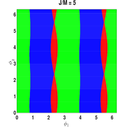
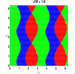
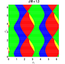
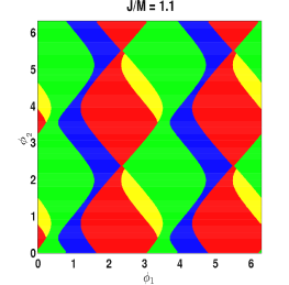
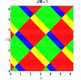
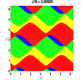
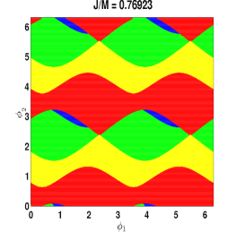
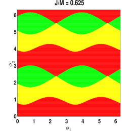
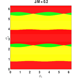
Figure 3: Phase diagrams of Eq. (32) for $J/M~{}=~{}5,~{}1.6,~{}1.3,~{}1.1,~{}1,~{}1/1.1,~{}1/1.3,~{}1/1.6$ and $1/5$. The different colors represent phases characterized by different number of Majorana modes at each end of a finite system in the fermion language and long-range ordering of different operators in the spin language. These phases correspond to A (yellow, two end Majorana modes, $\tau^{y}$ ordering), B (green, one end Majorana mode, $\sigma^{x}$ ordering), C (red, no end Majorana modes, $\tau^{x}$ ordering) and D (blue, one end Majorana mode with roles of $a$ and $b$ interchanged compared to phase B, $\sigma^{y}$ ordering). The panel at the bottom shows the colors of the four phases which would be in increasing shades of darkness in a black and white picture.

We see from Fig. 3 that only phases B (green) and D (yellow) survive for $J/M\to\infty$, and only phases A (blue) and C (red) survive for $J/M\to 0$. There is a critical value of $J/M=(1+\sqrt{5})/2\simeq 1.618$ above which phase A is completely absent. This is given by the fact that if the three roots $\lambda_{1}$, $\lambda_{2}$ and $\lambda_{3}$ all lie on or within the unit circle, then one can show that

$$\frac{J}{M}~{}=~{}\sqrt{\frac{(\lambda_{1}+\lambda_{2}+\lambda_{3})^{2}+(\lambda_{1}\lambda_{2}\lambda_{3})^{2}}{1+(\lambda_{1}\lambda_{2}+\lambda_{2}\lambda_{3}+\lambda_{3}\lambda_{1})^{2}}}$$ (40)

has a maximum value of $(1+\sqrt{5})/2$ corresponding to $(\lambda_{1},\lambda_{2},\lambda_{3})=(1,1,-(3-\sqrt{5})/2)$ or $(-1,-1,(3-\sqrt{5})/2)$. Similarly, there is a critical value of $J/M=(\sqrt{5}-1)/2\simeq 0.618$ below which phase D is completely absent. Hence the golden ratio determines the critical value of $J/M$ for hosting more than three phases.

The most complex figure corresponds to $J/M=1$. We see that the phase boundary lines correspond to straight lines crossing each other at $90^{o}$. This can be understood analytically as follows. On a phase boundary, we have $\lambda=e^{ik}$, with real $k$, in Eq. (37). If $k\neq 0$ or $\pi$, we can take the real and imaginary parts of the equation to obtain

$$(\nu+J_{y})~{}\cos(3k/2)~{}+~{}(\mu+J_{x})~{}\cos(k/2) = 0,$$

$$(\nu-J_{y})~{}\sin(3k/2)~{}-~{}(\mu-J_{x})~{}\sin(k/2) = 0.$$ (41)

Using the identities $\cos(3k/2)/\cos(k/2)=2\cos k-1$ and $\sin(3k/2)/\sin(k/2)=2\cos k+1$, we obtain $\cos k=(\nu+J_{y}-J_{x}-\mu)/(2(\nu+J_{y}))=(\mu-J_{x}+J_{y}-\nu)/(2(\nu-J_{y}))$. Eliminating $\cos k$ from the above equations, we find $J_{x}J_{y}-J_{y}^{2}~{}=~{}\mu\nu-\nu^{2}$. Using Eq. (39), we get $J~{}[\cos(2\phi_{1})+\sin(2\phi_{1})-1]=M~{}[\cos(2\phi_{2})+\sin(2\phi_{2})-1]$ For $J/M=1$, this gives the relationship

$$\sin(2\phi_{1}+\pi/4)~{}=~{}\sin(2\phi_{2}+\pi/4).$$ (42)

This implies that either $\phi_{2}=\phi_{1}+n\pi$ or $\phi_{2}+\phi_{1}=n\phi+\pi/4$, where $n$ is an integer. These describe some of the straight line phase boundaries that one sees in the figure for $J/M=1$. Some other straight lines in that figure come from the conditions that a single root lies at $\lambda=\pm 1$ (corresponding to $k=0$ or $\pi$); these give the conditions $\nu+J_{x}+\mu+J_{y}=0$ and $\nu-J_{x}+\mu-J_{y}=0$ respectively which, for $J/M=1$, give $\sin(\phi_{1}+\pi/4)=\pm\sin(\phi_{2}+\pi/4)$. These give some additional straight lines corresponding to $\phi_{2}+\phi_{1}=2n\pi\pm\pi/2$.

We have thus provided an explicit model of long-ranging hopping which has rich spin features and phase diagrams. The model supports phases that go beyond those of the Kitaev chain in their multiple Majorana structure.

V Broken Time-reversal Symmetry:  Complex Hopping and $\Delta$

In this section, we consider a different generalization of our model, one in which TRS is broken. As discussed in Sec. II B, this model belongs to a different symmetry class from that of the Kitaev chain, namely class D. We find that the fate of the zero energy modes, topology and Majorana structure is unusual in that TRS breaking yields a finite regime in the phase diagram that is gapless.

V.1 Model and Phases

Our model is described by the Hamiltonian

$$H~{}=~{}\sum_{n}~{}\Big{[}-wf_{n}^{\dagger}f_{n+1}-w^{*}f_{n+1}^{\dagger}f_{n}+\Delta f_{n}f_{n+1}+\Delta^{*}f_{n+1}^{\dagger}f_{n}^{\dagger}-\mu(f_{n}^{\dagger}f_{n}-1/2)\Big{]},$$ (43)

where $w$ and $\Delta$ may be complex. We now observe that $\Delta$ can be made real by a phase transformation of $f_{n}$ and $f_{n}^{\dagger}$, namely, changing $f_{n}\to f_{n}e^{i\theta}$ and $f_{n}^{\dagger}\to f_{n}^{\dagger}e^{-i\theta}$ changes the phase of $\Delta$ by $e^{i2\theta}$ without changing the phase of $w$. On the other hand, the phase of $w$ cannot be changed by any transformation without affecting the phase of $\Delta$. We can therefore assume without loss of generality that $\Delta$ is real. Writing $w=w_{0}e^{i\phi}$, where $w_{0}$ is real and positive, we obtain

$$H~{}=~{}\sum_{n}~{}\Big{[}-w_{0}e^{i\phi}f_{n}^{\dagger}f_{n+1}-w_{0}e^{-i\phi}f_{n+1}^{\dagger}f_{n}+\Delta(f_{n}f_{n+1}+f_{n+1}^{\dagger}f_{n}^{\dagger})-\mu(f_{n}^{\dagger}f_{n}-1/2)\Big{]}.$$ (44)

By making appropriate phase transformations, we can ensure that $\phi$ lies in the range $[0,\pi/2]$; we therefore study the properties of this model only within this range. If we use the Jordan-Wigner transformation in Eq. (17), we find that Eq. (44) takes the following form in terms of a spin-1/2 chain

$$H~{}=~{}-~{}\frac{1}{2}\sum_{n}\Big{[}(w_{0}\cos\phi-\Delta)\sigma_{n}^{x}\sigma_{n+1}^{x}~{}+~{}(w_{0}\cos\phi+\Delta)\sigma_{n}^{y}\sigma_{n+1}^{y}~{}+~{}w_{0}\sin\phi~{}(\sigma_{n}^{x}\sigma_{n+1}^{y}-\sigma_{n}^{y}\sigma_{n+1}^{x})~{}+~{}\mu\sigma_{n}^{z}\Bigl{]}.$$ (45)

In momentum space, we find that Eq. (44) takes the form given in the first equation in Eq. (25), where

$$h_{k}~{}=~{}(2w_{0}\sin\phi\sin k)~{}I~{}-~{}(2w_{0}\cos\phi\cos k~{}+~{}\mu)~{}s^{z}~{}+~{}(2\Delta\sin k)~{}s^{y}.$$ (46)

(Note that we have explicit TRS, $h^{*}_{-k}=h_{k}$, only if $\phi=0$ or $\pi$). The energy-momentum dispersion is given by

$$E_{k}~{}=~{}2w_{0}\sin\phi\sin k~{}\pm~{}\sqrt{(2w_{0}\cos\phi\cos k~{}+~{}\mu)^{2}~{}+~{}4\Delta^{2}\sin^{2}k}.$$ (47)

The quantum critical points (or lines) are given by the condition $E_{k}=0$ for some value of $k$ lying in the range $[0,\pi]$, namely,

$$(2w_{0}\cos\phi\cos k~{}+~{}\mu)^{2}~{}+~{}4\Delta^{2}\sin^{2}k~{}=~{}4w_{0}^{2}\sin^{2}\phi\sin^{2}k$$ (48)

for some $k$. To understand the complete phase diagram, we look at the quantum critical points for six values of $\phi$ in the range $[0,\pi/2]$. The resultant phase diagrams are shown in Fig. 4. For all values of $\phi$ (except for $0$ and $\pi/2$), the energy vanishes on two lines and within a two-dimensional region. The two quantum critical lines are given by the vertical lines $\mu/w_{0}=\pm 2\cos\phi$ (shown in red); on these lines, the energy vanishes at $k=0$ or $\pi$. The two-dimensional region (shown in blue) consists of a rectangle whose left and right sides are capped by elliptical regions. The rectangle is bounded by the horizontal lines given by $\Delta/w_{0}=\pm\sin\phi$ and the vertical lines $\mu/w_{0}=\pm 2\cos\phi$. Finally, the elliptical regions on the sides of the rectangle always touch the points $(\mu/w_{0},\Delta/w_{0})=(\pm 2,0)$.

So, to describe the evolution from the TRS preserved case ($\phi=0$) to the full broken case ($\phi=\pi/2$), at $\phi=0$, we have the phase diagram respected by the Kitaev chain (the first figure in Fig. 4). Topological phases exist vertically below and above the gapless line running from $(\mu/w_{0},\Delta/w_{0})=(-2,0)$ to $(2,0)$ while the region $|\mu/w_{0}|>2$ are non-topological. As seen in Fig. 4, as $\phi$ deviates from zero, the vertical phase boundaries ($\mu/w_{0}=\pm 2\cos\phi$) approach one another, the gapless line along $\Delta=0$ grows to a two-dimensional gapless regime that consists of a rectangular region between the vertical phase boundaries and two elliptical caps on the sides. By invoking adiabaticity, and as shown rigorously below, we find that the topological regions persist above and below the gapless regions, and are bound between the vertical phase boundaries while the rest of the gapped regime remains non-topological. Finally, upon reaching $\phi=\pi/2$ (the last figure in Fig. 4), the two vertical lines merge into a single line given by $\mu=0$, shrinking the topological region to non-existence and the two-dimensional region forms a single ellipse given by $\mu^{2}+4\Delta^{2}=4w_{0}^{2}$.

The gapless regions, shown in blue in Fig. 4, are quite unusual. For each value of $k$ (except 0 and $\pi$) and $\phi$, Eq. (48) describes an ellipse in the plane of $\mu/w_{0}$ and $\Delta/w_{0}$. The gapless regions arise when all the ellipses for different values of $k$ are combined. This is reminiscent of the Kitaev model of spin-1/2’s on a hexagonal lattice; that model also has a gapless region in which the energy vanishes at different points in the two-dimensional Brillouin zone kitaev2 .

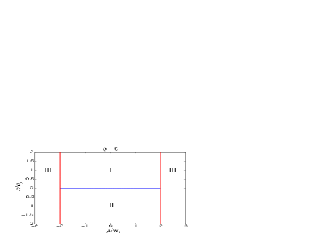
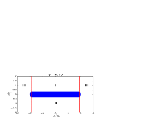
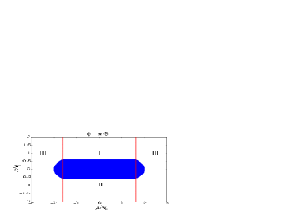
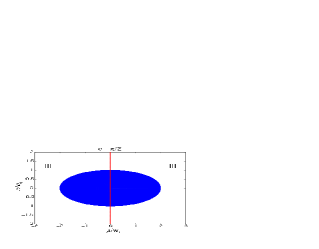
Figure 4: Phase diagrams of Eq. (44) as a function of $\mu/w_{0}$ and $\Delta/w_{0}$, for $\phi~{}=~{}0,~{}\pi/10,~{}\pi/5,~{}3\pi/10,~{}2\pi/5$ and $\pi/2$. The system is gapless on the vertical red lines and everywhere in the blue shaded regions. The figures show the phases I and II which are topological and phase III which is non-topological; the three phases exist in all the figures except for the bottom right figure ($\phi=\pi/2$) where phases I and II do not exist.

Turning to the fate of zero energy end modes, consider Eq. (44) expressed in terms of Majorana fermions:

$$H~{}=~{}-~{}\frac{i}{2}~{}\sum_{n}~{}\Big{[}w_{0}\cos\phi~{}(a_{n}b_{n+1}~{}+~{}a_{n}b_{n-1})~{}-~{}\Delta(a_{n}b_{n+1}-a_{n}b_{n-1})~{}+~{}\mu~{}a_{n}b_{n}~{}+~{}w_{0}\sin\phi~{}(a_{n}a_{n+1}~{}+~{}b_{n}b_{n+1})\Big{]}.$$ (49)

(Based on the time-reversal transformation of $a_{n}$ and $b_{n}$ discussed in Sec. IV B, we again see that that this Hamiltonian does not have TRS unless $\phi=0$ or $\pi$). The Heisenberg equations of motion following from Eq. (49) give

$$w_{0}\cos\phi~{}(b_{n+1}~{}+~{}b_{n-1})~{}-~{}\Delta~{}(b_{n+1}~{}-~{}b_{n-1})~{}+~{}\mu~{}b_{n}~{}+~{}w_{0}\sin\phi~{}(a_{n+1}-a_{n-1}) = 0,$$

$$w_{0}\cos\phi~{}(a_{n+1}~{}+~{}a_{n-1})~{}-~{}\Delta~{}(a_{n-1}~{}-~{}a_{n+1})~{}+~{}\mu~{}a_{n}~{}+~{}w_{0}\sin\phi~{}(b_{n-1}-b_{n+1}) = 0,$$ (50)

for the zero energy modes. Eqs. (50) show that the zero energy modes couple $a_{n}$ and $b_{n}$ if $\sin\phi\neq 0$, i.e., if TRS is broken. In terms of Fig. 4, we find that the the region lying between the two vertical lines but excluding the rectangular region forms a topological phase. In this phase, a long chain has one zero energy Majorana mode at each end; these modes have real wave functions (involving both $a_{n}$ and $b_{n}$), and they are separated from all the other modes by a finite energy gap. We have shown this using numerical calculations but we can also understand it analytically as follows.

Consider a general quadratic Majorana Hamiltonian of the form

$$H~{}=~{}i\sum_{m,n=1}^{2N}~{}c_{m}M_{mn}c_{n},$$ (51)

where $M$ is a real antisymmetric matrix; hence $iM$ is Hermitian. (For instance, this is the Hamiltonian we get for a $N$-site system if we define the operators $c_{n}$ in terms of $a_{n}$ and $b_{n}$ as $c_{2n-1}=a_{n}$ and $c_{2n}=b_{n}$ for $n=1,2,\cdots,N$). One can show that the non-zero eigenvalues of $iM$ come in pairs $\pm\lambda_{j}$ (where $\lambda_{j}>0$), and the corresponding eigenvectors are complex conjugates of each other, $x_{j}$ and $x^{*}_{j}$; this is because $iMx_{j}=\lambda_{j}x_{j}$ implies $iMx^{*}_{j}=-\lambda_{j}x^{*}_{j}$. The number of zero eigenvalues of $iM$ must be even, and one can choose those eigenvectors to be real: if $iMx_{j}=0$, we have $iMx^{*}_{j}=0$, and we can then obtain real eigenvectors by taking the linear combinations $x_{j}+x^{*}_{j}$ and $i(x_{j}-x^{*}_{j})$.

Now, let us consider a Hamiltonian with TRS which has, say, $q$ zero energy Majorana modes at the left end of a long chain. Let us assume that the bulk modes are gapped at zero energy, i.e., there are no bulk states with energies lying in the range $[-E_{0},E_{0}]$, where $E_{0}$ is a positive quantity. Next, let us add a small TRS breaking perturbation to the Hamiltonian. By adiabaticity, the $q$ zero energy modes at the left end continues to lie within the bulk gap, but they need not remain at zero energy. However, we know from the arguments in the previous paragraph, that they can only move away from zero energy in pairs. Hence, if $q$ is odd, one Majorana mode must remain at zero energy with a real eigenvector. Since we know from Sec. II A that the case with $\phi=0$, which has TRS, phases I and II are topological and have one Majorana mode at each end of a chain, this must continue to remain true if we make $\phi$ non-zero, as long as the bulk gap does not close. However, the nature of the end Majorana mode changes from the case with TRS (where it involves only $a_{n}$ or only $b_{n}$) to the case with broken TRS (where it involves both $a_{n}$ and $b_{n}$).

V.2 General Quadratic Majorana Hamiltonian and Topological Phases

As seen above, TRS breaking results in couplings of the $a$ fermions amongst themselves, and similarly couplings amongst the $b$ fermions. In this section, we will consider the most general Hamiltonian which is quadratic in terms of the Majorana fermions $a_{n}$ and $b_{n}$, thus generalizing the arguments presented in Sec. IV A (on long-range hopping) to include TRS breaking. This enables us to discuss the $\mathbb{Z}_{2}$-valued invariant which appears in such a system.

For an infinitely long chain, such a Hamiltonian can be written as

$$H~{}=~{}-i\sum_{r=-\infty}^{\infty}~{}\sum_{n=-\infty}^{\infty}~{}J_{r}~{}a_{n}b_{n+r}~{}-i~{}\sum_{r=1}^{\infty}~{}\sum_{n=-\infty}^{\infty}~{}[K_{r}~{}a_{n}a_{n+r}~{}+~{}L_{r}~{}b_{n}b_{n+r}],$$ (52)

where $J_{r},~{}K_{r},L_{r}$ are all real parameters. In momentum space, this can be written as in the first equation in Eq. (25), where

$$h_{k} = -2\sum_{r=-\infty}^{\infty}~{}[J_{r}~{}\cos(kr)~{}s^{z}~{}+~{}J_{r}\sin(kr)~{}s^{y}]$$ (53)

$$+~{}2~{}\sum_{r=1}^{\infty}~{}[(K_{r}+L_{r})~{}\sin(kr)~{}I~{}+~{}(K_{r}-L_{r})~{}\sin(kr)~{}s^{x}].$$

The energy-momentum dispersion is given by

$$E_{k} = 2~{}\sum_{r=1}^{\infty}~{}[(K_{r}+L_{r})~{}\sin(kr)$$ (54)

$$\pm~{}2~{}\sqrt{\left(\sum_{r=-\infty}^{\infty}~{}J_{r}~{}\cos(kr)\right)^{2}~{}+~{}\left(\sum_{r=-\infty}^{\infty}~{}J_{r}\sin(kr)\right)^{2}~{}+~{}\left(\sum_{r=1}^{\infty}(K_{r}-L_{r})~{}\sin(kr)\right)^{2}}.$$

We now observe that Eq. (53) has TRS, i.e., $h^{*}_{-k}=h_{k}$ for all $k$, only if $K_{r}=L_{r}=0$ for all $r$. In that case, as indicated in Secs. IV A-B, $h_{k}$ defines a vector in the $y-z$ plane as in Eq. (27); since this plane contains the origin, we have already seen that we can define a winding number around the origin as in Eq. (10), and this is a TI taking values in $\mathbb{Z}$ (the set of all integers). However, if some of the $K_{r}$ or $L_{r}$ are non-zero, then $h_{k}$ does not have TRS and has all four components (along $I,~{}s^{x},~{}s^{y}$ and $s^{z}$) in general; one cannot define a winding number around the origin for a closed curve (generated by $k$ going from 0 to $2\pi$) if the curve is in more than two dimensions. On the other hand, at $k=0$ and $\pi$, $h_{k}$ only has a component along $s^{z}$ given by $h(0)=-2\sum_{r}J_{r}$ and $h(\pi)=-2\sum_{r}(-1)^{r}J_{r}$ respectively. Thus, for the gapped regions in parameter space, we explicitly see that we can employ the bulk TI defined in Eq. (11), yielding

$$\nu_{bulk}=\mbox{sgn}\left(4\sum_{r}J_{r}\sum_{q}(-1)^{q}J_{q}\right).$$ (55)

This invariant takes the values $-1$ and 1 in the topological and non-topological phases respectively; its value cannot change unless either $h(0)$ or $h(\pi)$ crosses zero in which case the energy $E_{0}$ or $E_{\pi}$ must vanish. As an example, for the simple system with complex hopping discussed in the previous subsection, Sec. V.1, we see that $\nu_{bulk}=\mbox{sgn}(\mu^{2}-4w_{0}^{2}\cos^{2}\phi)$ is equal to $-1$ in the regions $|\mu|<2w_{0}\cos\phi$. Once we consider the fact that in this regime, the system is gapped only for $|\Delta|>2w_{0}\sin\phi$, the condition $\nu_{bulk}=-1$ captures the correct topological regions shown in Fig. 4.

To explicitly analyze the nature of the end Majorana modes, we have seen that in a system with TRS (with $K_{r}=L_{r}=0$) there can be any number of such modes at each end. For instance, Fig. 1 (e) shows a system in which only $J_{2}$ is non-zero and there are two zero energy modes at each end of an open chain shown by $a_{3}$, $a_{4}$, $b_{5}$ and $b_{6}$. However, if we now break TRS slightly by turning on small values of $K_{1}$ and $L_{1}$ in the Hamiltonian, i.e., introduce terms like $-iK_{1}a_{3}a_{4}-iL_{1}b_{5}b_{6}$, the energies of these modes shift away from zero to $\pm K_{1}$ and $\pm L_{1}$, destroying any zero energy Majorana modes. One can see an odd-even effect manifest in that if there are an odd number of zero energy Majorana modes at one end of the chain in the presence of TRS, breaking the symmetry would in general couple these modes. But given that there are an odd number of states and that the Hamiltonian only permits states to come in $\pm E$ pairs, unlike in the even case, one $E=0$ Majorana end mode has to survive.

To conclude, a system with TRS can have an arbitrary number of zero energy Majorana modes at each end of a long chain. If TRS is then broken, pairs of these end modes move away from zero energy. In general, therefore, we are left with either no Majorana modes or only one Majorana mode depending on whether the parent system with TRS has an even or an odd number of Majorana modes.

VI Spatially Varying Potentials

Having considered the effects of long-range hopping and TRS breaking on the topological features of the Kitaev chain, we now treat the effect of subjecting the chain to a spatially varying potential landscape. For the discretized lattice, the potential landscape can be described in terms of a site-dependent chemical potential. The last term containing the global chemical potential $\mu$ in Eq. (1) can be replaced by one having a local chemical potential $\mu_{n}$. The topology of such systems has been studied before adagideli ; shivamoggi ; sau ; ladder ; niu ; period ; tezuka ; lang ; motrunich ; brouwer1 ; lobos ; cook ; pedrocchi ; degottardi

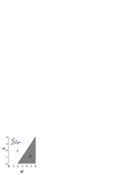
Figure 10: Topological phase diagram for a potential $\mu_{n}=W\cos\left(2\pi\omega n\right)$. The symbols $T$ and $N$ refer to topological and non-topological regions respectively.

The phase diagram in Fig. 4 (a) shows that in the the spatially homogeneous case, topological phases exist in the Kitaev chain even with arbitrarily small superconductivity present ($\Delta\neq 0$) and persist until a chemical potential $\mu$ that is of the order of the bandwidth $w$ is applied kitaev1 . Here we shall see that this is a singular limit and that for spatially varying potential these features no longer persist brouwer1 ; brouwer2 ; brouwer3 . In fact, in general we will see that for any finite potential, a minimum amount of superconductivity is required to reach the topological phase, though there remain interesting counterexamples to this general rule (see Fig. 10) motrunich .

In what follows, we analyze three different kinds of potential landscapes, expanding and building on our recent short work, Ref. degottardi . As the simplest example and a direct application of the transfer matrix techniques presented in Sec. II B, we obtain the phase diagram for periodic potentials having short periods commensurate with the lattice (see also  ladder ; niu ; period ). We then develop our transfer matrix further to enable an extensive study of more complex potentials. In particular, we provide a mapping between the normal state properties of the wire and its topology in the superconducting state. Our result is a more general form of the mappings presented in Refs. sau ; adagideli . However, this transformation becomes singular at $\Delta=1$, and thus cannot by itself be used to obtain the full phase diagram (see Sec. VI. B). The line $\Delta=1$ may be treated separately (this regime corresponds to the random field Ising model). We have also developed a mapping between the topology between the gap function $\Delta$ and $1/\Delta$. Taken together, these procedures allows us to obtain the topological phase diagram and the decay length of the end Majorana wave functions in terms of the normal state localization properties of the system. This mapping enables us to leverage the vast literature on the localization properties of 1D systems to the question of the topology of these systems in the presence of superconductivity.

Given the close connection between normal state properties and topology, we find that a great deal of insight can be gained by briefly reviewing the band structure of simple periodic systems, which is done in Sec. VI A. In Sec. VI B, the mapping between normal state properties and topology will be developed. Finally, Sec. VI C presents an application of these methods to ultra-long periodic and quasiperiodic potentials.

VI.1 Periodic Potentials and band structure

Given that we will forge a connection between the topological and normal state properties of inhomogeneous systems, it is helpful to review some basic properties of the normal state band structure ladder ; degottardi . The problem of an electron hopping in a periodic potential is described by Eq. (1) where we set $\Delta=0$ and take the chemical potential $\mu_{n}$ to depend on $n$ in a periodic way. For a state with energy $E$, we get the discrete form of the Schrödinger equation

$$-w(f_{n+1}+f_{n-1})-\mu_{n}f_{n}~{}=~{}Ef_{n},$$ (56)

This can be written in the transfer matrix form

$$\left(\begin{array}[]{c}f_{n+1}\\ f_{n}\end{array}\right)~{}=~{}\left(\begin{array}[]{cc}-\frac{1}{w}(E+\mu_{n})&-1\\ 1&0\end{array}\right)\left(\begin{array}[]{c}f_{n}\\ f_{n-1}\end{array}\right).$$ (57)

The energy spectrum consists of those values of $E$ which admit plane wave states, $f_{n}\sim e^{\pm ikn}$. For a system with period $q$, the appropriate object to consider is

$$\mathcal{A}=\prod_{n=1}^{q}\left(\begin{array}[]{cc}-\frac{1}{w}(E+\mu_{n})&-1\\ 1&0\end{array}\right).$$ (58)

Since $\mathcal{A}$ is $2\times 2$, its eigenvalues satisfy

$$\lambda^{2}-\left(\mbox{Tr}\mathcal{A}\right)\lambda+\mbox{det}\mathcal{A}=0.$$ (59)

Let $\lambda_{\pm}$ denote the two eigenvalues of $\mathcal{A}$. Since $\mbox{det }\mathcal{A}=1$, we have $\lambda_{+}\lambda_{-}=1$. Further, $\lambda_{+}+\lambda_{-}$ must be real. Hence

$$\lambda_{\pm}=\begin{cases}e^{\pm ir}~{}~{}~{}~{}~{}\mbox{for}~{}~{}|\mbox{Tr}~{}\mathcal{A}|~{}\leq~{}2,\\ e^{\pm r}~{}~{}~{}~{}~{}~{}\mbox{for}~{}~{}\mbox{Tr}~{}\mathcal{A}~{}>~{}2,\\ -e^{\pm r}~{}~{}~{}~{}\mbox{for}~{}~{}\mbox{Tr}~{}\mathcal{A}~{}<~{}-2,\\ \end{cases}$$

where $r$ is real. The object $\mbox{Tr}~{}\mathcal{A}$ is a $q^{th}$ order polynomial in $E$, and the spectrum of the system corresponds to the those values of $E$ for which $|\mbox{Tr}\mathcal{A}|\leq 2$. A useful quantity which quantifies the localization properties of the system is the Lyapunov exponent $\gamma(W)\equiv\lim_{\begin{subarray}{l}\mathcal{N}\to\infty\end{subarray}}\frac{1}{\mathcal{N}}\ln|\max(\lambda_{\pm})|$. Fig. 5 presents a detailed example of the normal state properties of a periodic system at zero energy as well as anticipating the connection between the normal state and the topological properties developed in Sec. IV B.

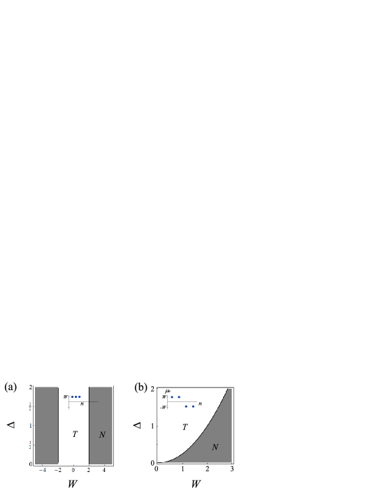
Figure 5: Topological phase diagram showing the topological ($T$) and non-topological ($N$) phases as a function of the potential strength $W$ and the superconducting gap $\Delta$ for (a) a uniform potential $\mu_{n}=W$, and (b) a periodic potential having the pattern $(W,W,-W,-W)$.

It is instructive to consider the case of simple periodic patterns as they offer a great deal of insight into the properties of the phase diagrams in more complicated situations. These features anticipate and provide qualitative understanding of our central results in subsequent sections. For instance, we will consider potentials of the form $\mu_{n}=W\epsilon_{i}$, where $\epsilon_{i}$ is some inhomogeneous potential of fixed strength and zero mean. A (very) naive caricature of such a system would be a period-2 potential of the form $\mu_{n}=...,-W,W,...$ or a period-4 potential $\mu_{n}=...,-W,-W,W,W,...$. The topology of these simple periodic patterns may be obtained by taking the transfer matrix $\mathcal{A}=\prod_{n=1}^{q}\mathcal{A}_{n}$ introduced in Sec. II B, where $q$ is the period of the potential. Given $\mathcal{A}$, TI $\nu$ may be straightforwardly found by applying the methods of Sec. II.2.2 and Eq. (16), in particular. Such simple periodic patterns naturally arise in a spin ladder model in which a vortex degree of freedom controls the sign of the chemical potential in the corresponding fermion system ladder , a one-dimensional version of Kitaev’s celebrated honeycomb model kitaev2 . Several simple examples are given in Fig. 5 and Table 2).

Table 2: Criteria for topological phases for a selection of periodic potentials (we have set $w=1$).

period	pattern	topological for
1	$\ldots,W,W,W,\ldots$	$|W|<2$
2	$\ldots,W,-W,\ldots$	$\Delta>|W|/2$
4	$\ldots,W,W,W,-W,\ldots$	$\Delta^{2}>W^{2}/2-1$
4	$\ldots,W,W,-W,-W,\ldots$	$\Delta>W^{2}/4$

The presence of a phase offset in commensurate periodic potentials can significantly affect the topological phase diagram. As an illustrative example, let us consider the period-4 pattern given by

$$\mu_{n}=\sqrt{2}\mu\cos\left(\frac{\pi}{4}(2n+1)+\phi\right).$$ (60)

Since shifting $\phi\to\phi+\pi/2$ is equivalent to shifting $n\to n+1$, it is sufficient to study this problem in the range $0\leq\phi\leq\pi/2$. Upon finding the eigenvalues of the product of four transfer matrices $A_{4}A_{3}A_{2}A_{1}$ of the form given in Eq. (62) below, we find that the phase boundary between the topological and non-topological phases is given by

$$4\sqrt{2}|w\Delta|=\mu^{2}\sqrt{1+\cos(4\phi)}.$$ (61)

The phase diagram is shown in Fig. 6. The fact that the boundary between the topological and non-topological phases diverges in $\mu$ as $\phi\to\pi/4$ can be understood as follows. For $\phi=0$, we know that the pattern of the chemical potential takes the form $P=++--...$ and thus has the phase boundary given by $\mu=2\sqrt{|w\Delta|}$ (see the last line of Table I). For $\phi=\pi/4$, the pattern assumes the form $Q=+0-0+...$. In the limit $\mu\to\infty$ (in which the hopping plays no role), the eigenstates of the system are localized to each site. Given that $\mu=0$ at every other site, the system must contain bound Majorana modes and therefore must be topological. The general shape of the phase boundary then follows from the fact that it connects the points $(2\sqrt{|w\Delta|},0)$ and $(\infty,\pi/4)$ in the $(\mu,\phi)$ plane. In general we conjecture that for any periodic pattern, $\mu_{n}=\mu\cos(\pi Qn+\phi)$ where $Q$ is a rational number, if the chemical potential vanishes at certain sites for some value of $\phi$, a ‘finger’ of the topological phase will extend up to $\mu=\infty$ for that value of $\phi$. As will be seen in the next section, the sensitivity of the phase diagram to potentials vanishing at certain sites is quite ubiquitous and results in a non-analytic behavior of the phase boundary for disordered systems.

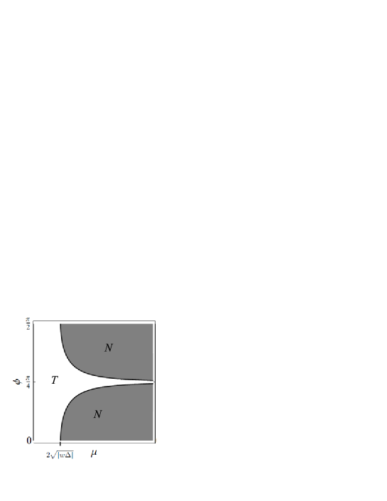
Figure 6: Topological phase diagram for a period-4 potential, showing the topological ($T$) and non-topological ($N$) phases as a function of $\mu$ and $\phi$.

VI.2 Mapping to Normal Systems and Duality

As observed in Ref. motrunich , the product of such transfer matrices, $\mathcal{A}\equiv\prod_{n=1}^{\mathcal{N}}A_{n}$, is strongly reminiscent of that used to determine localization properties of the normal state Anderson disorder problem, i.e. Eq. (57). We build on this observation by explicitly mapping the topological phase diagram to the normal state properties of the system (similar to a procedure developed in sau ). This mapping is performed in two steps. The first allows us to determine topological regions in the superconducting system in the range $0<\Delta<1$ based on a knowledge of its normal counterpart (same spatially varying potential but no superconductivity). The second is a duality which relates the topological phase diagram for a given superconducting gap $\Delta$ to that corresponding to strength $1/\Delta$. Taken together, these provide a complete mapping between the normal state and the topology of the superconducting system.

Mapping to Normal Systems – In Sec. II B, we introduced the transfer matrix relevant to a superconducting wire having spatially varying potentials:

$$A_{n}=\left(\begin{array}[]{cc}-\frac{\mu_{n}}{\Delta+w}&\frac{\Delta-w}{\Delta+w}\\ 1&0\end{array}\right).$$ (62)

For $0<\Delta<1$, we perform a similarity transformation $A_{n}=\sqrt{\delta}S\tilde{A}_{n}S^{-1}$ with $S=\mbox{diag}(\delta^{1/4},1/\delta^{1/4})$ and $\delta=\frac{1-\Delta}{1+\Delta}$. The matrices $\tilde{A}_{n}$ are of the form shown in Eq. (14) with $\Delta\to 0$ and $\mu\to\mu_{n}/\sqrt{1-\Delta^{2}}$. This immediately gives

$$\mathcal{A}(W,\Delta)=\left(\sqrt{\frac{1-\Delta}{1+\Delta}}\right)^{\mathcal{N}}S\mathcal{A}\left(W/\sqrt{1-\Delta^{2}},0\right)S^{-1}.$$ (63)

Taking the logarithm of the eigenvalues of Eq. (63), the condition that $|\lambda_{2}|=1$ is given by

$$\gamma(W,\Delta)=\gamma\left(\frac{W}{\sqrt{1-\Delta^{2}}},0\right)-\frac{1}{2}\ln\left(\frac{1+\Delta}{1-\Delta}\right),$$ (64)

reminiscent of a result in sau , where we have defined the Lyapunov exponent $\gamma(W,\Delta)\equiv\lim_{\begin{subarray}{l}\mathcal{N}\to\infty\end{subarray}}\frac{1}{\mathcal{N}}\ln|\lambda_{2}(W,\Delta)|$; the Lyapunov exponent is the inverse of the localization length, $\gamma(W,\Delta)=1/\ell(W,\Delta)$. In the limit $\gamma(W,\Delta)\to 0$, the system is gapless and Eq. (64) describes the phase boundary separating the topological and non-topological regions of the phase diagram. This relation quantifies the observation in motrunich ; brouwer2 that in general a critical amount of superconductivity must be applied before the system is driven into a topological phase. For the case in which the system is metallic (i.e., $\gamma(W,0)=0$), any non-zero $\Delta$ will give rise to a topological phase.

If $\mu_{n}=0$ for all $n$, we see from Eq. (62) that all the $A_{n}$ are identical and have both eigenvalues less than 1 in magnitude if $\Delta>0$ (we are assuming that $w>0$). This implies that $\gamma(W=0,\Delta)<0$. Thus the line $W=0$ and $\Delta>0$ will always lie in the topological phase.

Duality – The similarity transformation (Eq. (63)) is only valid in the range $0<\Delta<1$. The form of the phase diagram for $\Delta>1$ may be obtained by noting that the transformation

$$\mu_{n}\to\mu_{n}/\Delta,~{}~{}\Delta\to 1/\Delta,~{}~{}\mbox{and}~{}~{}P\to\tilde{P}$$ (65)

$$\mbox{where}~{}~{}P\to\tilde{P}:~{}\{\mu_{n}\}\to\{(-1)^{n}\mu_{n}\},$$

leaves the eigenvalues of $\mathcal{A}$ unchanged for $\mathcal{N}$ even. Thus, if a point $(W_{0},\Delta_{0}<1)$ lies on the phase boundary of $P$, then $(W_{0}/\Delta_{0},1/\Delta_{0})$ lies on the phase boundary of $\tilde{P}$. This duality strongly constrains the form of the phase boundary in the cases in which the distribution is invariant under the transformation in Eq. (65).

An interesting illustration of this duality is provided by the periodic patterns in Table 2. For example, note that the uniform case (period 1) and the period 2 case are dual to each other. Indeed, taking $\Delta\to 1/\Delta$ and $W\to W/\Delta$ for the equation $W=2$ (phase boundary for period 1 case), we obtain the phase boundary $\Delta=W/2$, appropriate for the period 2 case. Similarly, the two period 4 patterns are self-dual. For instance, taking $\Delta^{2}=W^{2}-1$, and applying $\Delta\to 1/\Delta$ and $W\to W/\Delta$ gives $1/\Delta^{2}=W^{2}/\Delta^{2}-1$ which is equivalent. The same holds true for $\Delta=W^{2}/4$.

Random-field quantum Ising Chain – Finally, at the point $\Delta=1$, the system maps to the quantum Ising chain subject to a spatially varying transverse field. As can be seen in Sec. II.3, the Jordan-Winger transformation applies even when the local chemical potential $\mu_{n}$ has a spatial dependence and appears as a spatially varying field along the $z$-direction. Along the line $\Delta/w=1$, we have $J_{y}=0$, and thus for a random distribution of $\mu_{n}$, the system corresponds to the 1D random transverse field Ising model, which has been studied in great depth fisher ; shivamoggi . The matrix $\mathcal{A}(W,1)$ has the eigenvalues $\frac{1}{2^{\mathcal{N}}}\prod_{n=1}^{\mathcal{N}}\mu_{n}$ and 0. Eq. (16) reveals that the phase boundary passes through the point for which

$$\langle\ln|\mu_{n}|\rangle=\ln 2,$$ (66)

where $\langle\ln|\mu_{n}|\rangle\equiv\lim_{\mathcal{N}\to\infty}\frac{1}{\mathcal{N}}\sum_{n=1}^{\mathcal{N}}\ln|\mu_{n}|$.

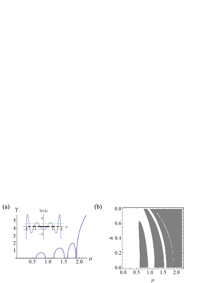
Figure 7: (a) Plot of the Lyapunov exponent $\gamma(\mu)$ for a period 10 potential with $\mu_{n}=\mu$ for $n=0$ mod 10 and $-\mu$ otherwise. Inset shows Tr $\mathcal{A}$. The allowed plane wave states (corresponding to $\eta(\mu)=0$) have $|\mbox{Tr }\mathcal{A}|\leq 2$. (b) The $\mu$-$\Delta$ topological phase diagram (topological region indicated in white, non-topological region in gray). Note that the values of $\mu$ for which $\gamma(\mu)=0$ in (a) are precisely those regions which become topological for arbitrarily small $\Delta$. This relationship is elucidated in Sec. VI B.

VI.3 Ultra-long Period and Quasiperiodic Potentials

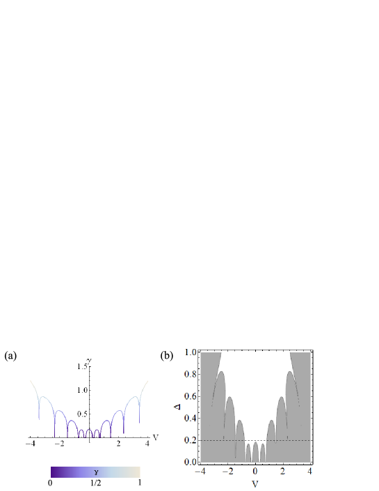
Figure 8: (a) The Lyapunov exponent $\gamma$ of the normal state ($\Delta=0$) for $\mu_{n}=V+2\cos\left(2\pi\omega n\right)$ with $\omega=1/10$. (b) Topological phase boundary showing the merging of the topological regions as described in the text. For $\Delta\ll 1$, there are are 10 distinct regions which are topological. At $\Delta=0.2$, the four central regions have merged to form a single region.

Building on our work in Sec. VI A, we consider periodic potentials of the form $\mu_{n}=B\cos\left(2\pi\omega n-\theta\right)$ but now allow the period of the potential ($q$, for $\omega=2\pi p/q$, for $p,q\in\mathbb{N})$) to be either very long or infinite tezuka ; lang . The Hamiltonian formed from this potential is known as the almost Mathieu operator. For $B=2$, the resultant equations of motion are known as Harper’s equations and arise in the context of a charged particle moving on a 2D square lattice in the presence of an external magnetic field hofstadter .

For $\omega$ irrational, the associated normal state energy spectrum is a fractal known as Hofstadter’s butterfly hofstadter . This fractal structure arises from a property of the quantity Tr $\mathcal{A}$ (with $\Delta=0$, see Sec. VI A) for the operator $\mu_{n}=2\cos\left(2\pi\omega n-\theta\right)$ (see Eq. (14)). This operator has the special property that for $\omega=p/q,p,q\in\mathbb{N}$, there are $q$ distinct bands hofstadter . This is a special property of Harper’s equation. For instance, note that in Fig. 7, although $q=10$, only 5 distinct bands exist. In contrast, Fig. 8 shows that all $q=10$ bands are present for Harper’s equation. For example, if we imagine letting $\omega\rightarrow\sqrt{2}$ by taking a sequence of better and better rational approximations, the number of bands will grow without bound. This is the origin of the unusual point-set topology of the spectrum for irrational $\omega$. A plot of the allowed bands as a function of the energy and $\omega$ leads to a fractal known as Hofstadter’s butterfly hofstadter . The general features of Hofstadter’s butterfly maybe seen in Fig. 9(a). Indeed, for $\omega$ irrational, the total ‘length’ associated with the spectrum is zero (by length, we mean $\int f(V)dV$, where $f$ is 1 if $V$ corresponds to a point in the spectrum, 0 if not). Formally, the Lebesgue measure of the almost Mathieu operator is $|4-2|B||$ last . Very roughly, as $q\to\infty$ for $B=2$, the length of the spectrum (as a function of energy) is zero, although there are still an infinite number of distinct bands! These seemingly paradoxical properties are the features of a so-called Cantor set.

These remarkable properties lead us to consider the topology of a 1D system subject to a potential of the form

$$\mu_{n}=V+2\cos\left(2\pi pn/q\right).$$ (67)

The allowed zero energy plane wave states in the $\omega-V$ plane correspond to Hofstadter’s butterfly. Of interest are the properties of the topological phase diagram as $\Delta$ is ‘turned on’. This problem is easily solved given the Lyapunov exponent $\gamma$ of Harper’s equation which we have plotted in Fig. 9(a). This plot is different from the usual plot of Hofstadter’s butterfly in that it shows the value of the Lyapunov exponent $\gamma$ rather than just the spectrum (the spectrum corresponds to points for which $\gamma=0$). Indeed, a feature of this plot are characteristic horizontal striations, which show the sensitivity of the localization length to the period of the potential ($q$).

We begin by considering the topological properties of a potential with a given $\omega$. Fig. 8 plots the Lyapunov exponent of a particular potential ($\omega=1/10$) as a function of $V$. As shown in Fig. 8(b), for the same potential and $\Delta\ll 1$, there are $q$ topological regions inherited from the normal state. These distinct regions fuse as $\Delta$ is increased. The precise value of $\Delta$ for which two topological regions merge is determined by the strength of the Lyapunov exponent between the gaps. Since this quantity tends to be larger for larger $|V|$, the gaps closer to $V=0$ tend to merge before those with larger $|V|$. We now generalize to the full $\omega-V$ space. As expected from our general analysis, the normal state properties (Fig. 9(a) directly inform the topological phase diagram (Fig. 9(b). We see that as superconductivity is increased, Hofstadter’s butterfly is ‘filled in’ by non-topological regions. The value of $\Delta$ at which the system becomes topological is extremely sensitive to the period $q$ of the potential.

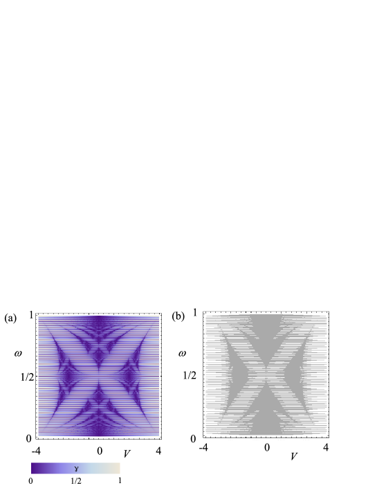
Figure 9: (a) A colorscale plot of $\gamma(V,0)$ for $\omega=n/200$, $0<n\leq 200$. Darker regions correspond to smaller values of $\gamma$. The characteristic striations show the spectrum’s sensitivity to the period of the potential; i.e., small changes in $\omega$ can lead to large changes in the period (which is given by $q$, where $\omega=p/q$, with $p$ and $q$ relatively prime). The resulting figure is reminiscent of the fractal known as Hofstadter’s butterfly. (b) The topological phase diagram for $\Delta=1/5$ mimics the low-lying values of $\gamma$ in (a).

The case of Harper’s equation allows us to study the crossover exhibited from periodic to quasiperiodic potentials. We now consider the case $\mu_{n}=W\cos\left(2\pi\omega n\right)$ with $\omega$ being irrational. The normal state features of this potential have been well-studied; the system is metallic (i.e., there are plane wave states at $E=0$) for $W<2$ and exhibits a metal-insulator transition at the critical value $W=2$ svetlana . The normal state Lyapunov exponent takes the form $\gamma(W,0)=\ln\left(W/2\right)$ for $W>2$ and $0$ for $0\leq W\leq 2$ for $\omega$ irrational delyon ; andre . Eq. (64) then predicts a topological phase for

$$\Delta>\frac{1}{2}W-1.$$ (68)

This result holds for all values of $\Delta>0$ given that the transformation $\omega\to\omega+1/2$ yields Eq. (65) and that the duality transformation, $\Delta\to 1/\Delta$ and $W\to W/\Delta$, leaves Eq. (68) invariant. Finally, Eq. (66) also shows that the point $(W,\Delta)=(4,1)$ lies on the phase boundary.

VII Disordered Potentials

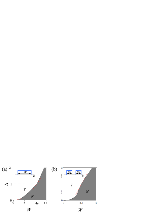
Figure 11: Topological phase diagrams for (a) box and (b) double box potentials. The red dotted lines indicate that at $\Delta=1$, the slope of the phase boundary, $d\Delta/dW$, has a discontinuity in (a) but is continuous in (b).

The topic of disordered superconducting wires that break the SU(2) symmetry associated with spin, namely those of the symmetry classes D and BDI discussed in previous sections, has been actively researched for over a decade altland ; brouwer1 ; gruzberg ; fidkowski1 . One of the highlighting features of these systems is that their symmetry properties greatly alter localization physics. In particular, while Anderson localization dictates that states are always localized in one-dimension in the presence of even the weakest disorder, these systems allow for the presence of a critical disorder point in parameter space that permits a delocalized state at zero energy altland ; brouwer1 ; gruzberg ; fidkowski1 . The point acts as a mobility edge in that it separates two localized regimes. In these systems, a variety of approaches have probed the manner in which the density of states diverges at zero energy, odd-even effects for coupled chains, and conduction properties (since charge is not a conserved quantity for excitations about the superconducting ground state, one studies thermal insulating/conducting properties). In pioneering work by Motrunich et al. motrunich , it was shown that the localized phases separated by the delocalized point are fundamentally different from one another. One phase supports end Majorana modes while the other does not, consistent with the classification of the phases as topological and non-topological, respectively, as in the disorder-free case.

Recent studies have focused on this feature of the presence of Majorana edge modes in the context of disordered systems shivamoggi ; sau ; brouwer1 ; brouwer2 ; brouwer3 ; beenakker ; adagideli ; degottardi . Along these lines, here we exploit the transfer matrix techniques that we have developed in previous subsections to pinpoint the conditions for the existence of these end modes in a full range of models of disorder and disorder strength. The map made to normal systems in Sec. VI B allows us to borrow extensively from literature on Anderson localization and perform a comprehensive study. We derive general features of the phase boundary for disordered superconducting systems, including a characteristic discontinuity of the phase boundary at the point associated with the random field Ising model ($\Delta=1$). We also obtain topological phase diagrams for a variety of disorder distributions based on our mapping to an extensive range of known results from Anderson localization studies of normal systems.

VII.1 Setup and General Results

We consider Eq. (1) with $\mu$ replaced by a spatially dependent $\mu_{n}$. The $\mu_{n}$ is drawn from some distribution and is uncorrelated, i.e. $\langle\mu_{n}\mu_{n^{\prime}}\rangle=U\delta_{n,n^{\prime}}$ and $\langle\mu_{n}\rangle=0$. The quantity $U$ is the standard deviation of the disorder and thus characterizes its strength.

For weak disorder, the Lyapunov exponent may be obtained from perturbation theory for the normal state system derrida ; disorderreview and is given by

$$\gamma(W,\Delta=0)=\left(\frac{\Gamma(3/4)}{\Gamma(1/4)}\right)^{2}U.$$ (69)

Applying Eq. (64), we obtain the condition for the topological phase

$$\Delta>\left(\frac{\Gamma(3/4)}{\Gamma(1/4)}\right)^{2}U\approx 0.114~{}U.$$ (70)

This result may be compared to that of a continuum model based on the Dirac equation, which gives a non-topological phase for $\Delta>\frac{1}{8}U=0.125U$ (see Ref. brouwer2 ). For disorder distributions that are symmetric around 0, the self-duality condition $P=\tilde{P}$ in Eq. (65) is satisfied. In this case, we can employ this duality transformation, $\Delta\to 1/\Delta$ and $U\to U/\Delta^{2}$, to show that Eq. (70) also describes the phase boundary in the limit of strong disorder. Finally, we mention that near the Ising point ($\Delta=1$), the disorder may give rise to a discontinuity in the phase diagram. We describe the physics of this phenomenon in the examples given now.

VII.2 ‘Box’ Disorder

As a generic representative for disorder, we now turn to the case of ‘box’ disorder for which the probability of $\mu_{n}$ falling at any point in the range $-W/2\leq\mu_{n}\leq W/2$ is equally likely. The low-energy behavior as shown in the numerical simulation in Fig. 11(a) is in good agreement with Eq. (70) (for box disorder, $U=W^{2}/12$). Eq. (66) reveals that the phase boundary passes through the point $(W,\Delta)=(W_{c},1)$, where $W_{c}=4e\approx 10.873$ (box disorder) with $e$ being the base of the natural logarithm.

Discontinuity of phase boundary– A noteworthy find is the observed discontinuity suffered by the phase boundary as it passes through the random transverse Ising field point $\Delta/w=1$ discussed in the previous section (Figs. 11(a) and 12). We can calculate the phase boundary near $\Delta/w\approx 1$ by noting that according to Sec. VI.2, $\gamma\left(\frac{W}{\sqrt{1-\Delta^{2}}},0\right)$, the effective Lyapunov exponent that we seek in Eq. (64), corresponds to that of very strong disorder for $\Delta\to 1$. In this limit, we can use the known form of the normal state Lyapunov exponent for $W\gg 1$

$$\gamma(W) \sim \ln\left(W/2+\sqrt{W^{2}/4-4}\right)-\sqrt{W^{2}/4-4}-\ln 2,$$ (71)

$$\sim \ln\left(W/2\right)-1+4/W^{2}+\mathcal{O}\left(1/W^{4}\right),$$

(there is a typo in the expression given in  disorderreview ). Substituting this expression into Eq. (64) and invoking self-duality, we obtain the phase boundary (to linear order around $(W,\Delta)=(4e,1)$))

$$\Delta\approx\begin{cases}\frac{e}{2e^{2}+2}W-\frac{e^{2}-1}{e^{2}+1}\ \ \mbox{for }\Delta\leq 1,\\ \frac{e}{2e^{2}-2}W-\frac{e^{2}+1}{e^{2}-1}\ \ \mbox{for }\Delta\geq 1.\end{cases}$$ (72)

As seen in Fig. 11(a), this result is in reasonable agreement with numerical simulations.

In order to understand the origin of this discontinuity, we investigate the phase boundary by performing perturbation theory in the quantity $(1-\Delta^{2})$. A straightforward calculation shows that the eigenvalues of the matrix $\mathcal{A}$ are 0 and

$$\lambda=\frac{1}{(1+\Delta)^{N}}\prod_{n=1}^{N}\mu_{n}\left[1+\left(1-\Delta^{2}\right)\sum_{m}\frac{1}{\mu_{m}\mu_{m+1}}+\left(1-\Delta^{2}\right)^{2}\sum_{m<m^{\prime}}\frac{1}{\mu_{m}\mu_{m+1}\mu_{m^{\prime}}\mu_{m^{\prime}+1}}+...\right].$$ (73)

From this expression, it is straightforward to obtain the Lyapunov exponent in terms of the disorder distribution. Letting $\Delta=1+\delta$, we get

$$\gamma=\langle\ln\mu\rangle-\ln 2-\frac{1}{2}\left(1+4\langle 1/\mu\rangle^{2}\right)\delta$$ (74)

up to order $\delta^{2}$. Let us define $\tilde{\delta}=\frac{1-\Delta}{1+\Delta}$; we then get that the phase boundary for $\tilde{\delta}\approx 0$ obeys

$$\langle\ln|\mu_{n}|\rangle=\ln 2-\left(1+4\langle 1/\mu\rangle^{2}\right)\tilde{\delta}+\mathcal{O}(\tilde{\delta}^{2}).$$ (75)

This shows that the phase boundary is fragile towards singularities when $\mu_{n}$ is allowed to come arbitrarily close to zero. Indeed, our simulations have shown that the discontinuity is absent for disorder distributions that avoid zero energy. A large class of disorder distributions that cover zero energy give rise to a discontinuity in the slope of the topological phase boundary at $\Delta=1$. This is another manifestation of the sensitivity that the phase diagram shows to $\mu_{n}$’s which are equal to zero (for example, see Eq. (66) or Fig. 7).

VII.3 Other forms of disorder

‘Double Box’ Disorder– A useful test of our hypothesis on the fragility of the phase boundary for arbitrarily small values of $\mu_{n}$ is to examine a system for which the disorder distribution excludes $\mu_{n}=0$ and thus we expect that the phase boundary be continuous near $\Delta=1$. Consider the following distribution for the local chemical potential, $\mu_{n}$:

$$f_{DB}(x;W)=\begin{cases}\frac{2}{W}\ \ \mbox{for }W/4\leq|x|\leq W/2,\\ 0\ \ \mbox{otherwise}.\end{cases}$$ (76)

Here, $W_{c}=2e\approx 5.437$. Note that all the $\langle 1/\mu^{n}\rangle$ exist. We can find the behavior of the phase diagram near $\Delta=1$ using Eq. (75). More directly however, we note that to linear order near $\Delta=1$, the only expression which is invariant under Eq. (65) is

$$\Delta=\alpha W-1.$$ (77)

This expression well describes the phase boundary for $\alpha=1/e$. This phase diagram is shown in Fig. 11(b) and is in good agreement with this prediction, in particular, being devoid of the singularity at $\Delta=1$.

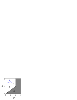
Figure 12: Topological phase diagram for Lorentzian disorder.

Lorentzian Disorder– Finally, we turn to the specific case of disorder which is unbounded and has a diverging standard deviation, the Lorentzian case. The distribution of local chemical potential is drawn from a distribution of the form

$$f_{L}(x;W)=\frac{1}{\pi}\frac{W}{x^{2}+W^{2}}.$$ (78)

The phase diagram is exactly soluble in this case since the normal state density of states is known exactly lloyd . The zero-energy Lyapunov exponent, first obtained by Thouless thoulessdos , takes the form $\gamma_{L}(W,0)=\ln\left(W/2+\sqrt{1+W^{2}/4}\right)$. Once again invoking Eq. (64) and self-duality of the phase diagram yields a phase boundary

$$W=\begin{cases}2\Delta\ \ \mbox{for }\Delta\leq 1,\\ 2\ \ \mbox{for }\Delta\geq 1.\end{cases}$$ (79)

This result, as shown in Fig. 12, is in excellent agreement with numerical simulations. It should be pointed out that the features of this phase diagram are extremely unusual. For instance, Eq. (70) fails to hold because the second moment $\langle\mu_{n}^{2}\rangle$ is ill-defined for $f_{L}$. This example is noteworthy since, for $W>2$ the system is always in a non-topological phase; no amount of $\Delta$ can drive the system topological. Studying these examples has shown us, among other features, that typically the larger the disorder, the more superconductivity is required for Majorana end modes to exist, and that the topological phase diagram is highly sensitive to the nature of the disorder distribution.

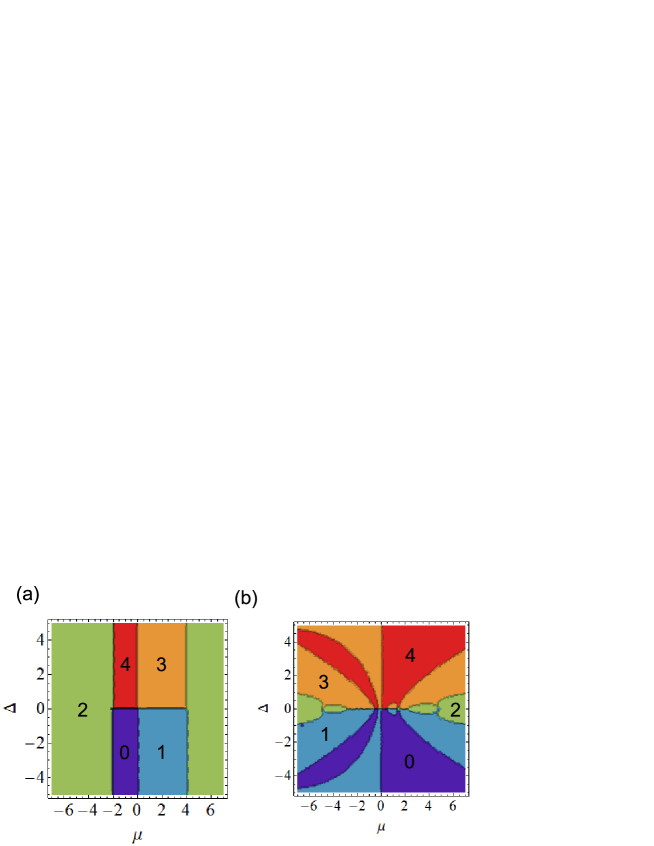
Figure 13: (a) The topological phase diagram of a uniform class BDI system (for which $\Delta$ is constrained to be real) described by Eq. (20) with $J_{0}=\mu/2$, $J_{1}=J_{2}=(w-\Delta)/2$, and $J_{-1}=J_{-2}=(w+\Delta)/2$, with $w=1$. That is, the system is similar to Eq. (1) but with next-nearest neighbor hopping and superconductivity equal to $w$ and $\Delta$. The different regions are labeled according to the topologically protected quantity $n_{f}$, which reflects the Majorana end mode structure as defined in Eq. (15). The phase diagram was obtained using the method presented in Sec. II.2.2. (b) The same phase diagram for a 15-site system with a $\mu_{n}=\mu V_{n}$, where $V_{n}$ is a random real variable between $-1$ and $1$.

We also mention that the method presented here may be applied to a Guassian distribution of disorder where a closed form of the Lyapunov exponent is known (see adagideli for an analysis of this example). However, the result involves Airy functions and is quite complex and we omit this example given that it has the same qualitative behavior as the phase boundary for ‘box’ disorder.

Future Directions – A very natural next step would be to consider spatially inhomogeneous potentials for a system in class BDI. The interplay between such potentials and phases exhibiting multiple Majorana modes should be quite rich. We offer a hint of this in Fig. 13. The figure indicates the intricate behavior which may occur in such cases, including re-entrant phases. Given this exciting behavior, we note that applied potentials offer a very promising route for the engineering of topological phase diagrams. We note however that the simple numerical methods which were applied here for a disordered system ($L\sim 10^{4}$) with nearest neighbor hopping will not work for systems with longer range hopping. This is due to the difficulty in extracting all the eigenvalues of a large product of matrices (and not just the largest one).

VIII Summary and Discussion

In this work we have presented a comprehensive study towards enhancing our understanding of topological phases of one-dimensional superconducting systems, TIs and Majorana end modes. We began with reviewing a prototypical model, the Kitaev chain, which describes spinless electrons hopping with an amplitude $w$ between the sites of a lattice, $p$-wave superconducting order (denoted by a parameter $\Delta$), and an on-site chemical potential $\mu$. This model has attracted a great deal of attention as the simplest model which exhibits topological phases and non-topological phases depending on the parameters appearing in the Hamiltonian. In the topological phases, a long chain with open boundary conditions has one zero energy mode localized at each end. The non-topological phase has no end modes. The model can be mapped, using the Jordan-Wigner transformation, to a spin-1/2 chain with $XY$ couplings and a magnetic field applied along the $z$ direction. There are two topological phases which have long-range order in the $x$ or $y$ components of the spin, while the non-topological phase does not have any long-range order.

Next, we showed that there are a number of TIs which can be used to characterize the different phases for uniform systems. There are different invariants depending on whether the system is time-reversal symmetric or not, commonly referred to as belonging to symmetry classes BDI and D, respectively. The TIs can be defined by invoking the bulk or the boundary properties for a large system with periodic and open boundary conditions respectively. For time-reversal symmetric systems, the bulk invariant is a $\mathbb{Z}$-valued winding number obtained from a closed curve lying in a two-dimensional plane, formed by the set of Hamiltonians spanning momentum space. If time-reversal symmetry is broken, the closed curve no longer lies in a plane and a winding number cannot be defined. However, the Hamiltonians at the points $k=0$ and $\pi$ can be used to define a $\mathbb{Z}_{2}$-valued invariant which can take values $\pm 1$. As for boundary invariants, based on the Heisenberg equations of motion for open chains, we obtained TIs that count the number of Majorana modes (whose components we explicitly argued to be real) at the ends of the system as well as their parity. We showed that in the presence of time-reversal symmetry breaking terms, multiple Majorana modes, while perhaps confined to the ends, disappear by obtaining complex components and moving away from zero energy, thus allowing at most a single Majorana mode at each end. We illustrated the bulk-boundary correspondence which relates the values of the bulk and boundary invariants to each other.

While the Hamiltonian for a Kitaev chain involves only nearest-neighbor hoppings and an on-site potential term, both only have interconnections between two types of Majorana fermions, $a$ and $b$, we generalized this model in several ways. First, we introduced long-range hoppings of the Majorana fermions to construct time-reversal symmetric models which can have any value of the $\mathbb{Z}$-valued TI in the bulk, and therefore any number of Majorana end modes. For a time-reversal symmetric system, we found that each end mode is purely of type $a$ or type $b$. As an illustration of the kind of rich phase diagram that one may have with long-range hoppings, we considered a particular model in detail. This model has four terms in the Hamiltonian one of which describes a next-nearest neighbor hopping. The model has four phases with the number of end modes of types $a$ and $b$ varying from zero to 2. The model can be mapped to a spin-1/2 chain; the corresponding model enjoys a complete duality. All the four phases have long-range order in terms of $x$ and $y$ components of either the original spins or the dual spins; the phases are related pair-wise to each other through duality. Second, we introduced time-reversal breaking hoppings of Majorana fermions on nearest-neighbor sites. We again obtained topological and non-topological phases depending on the parameters. The topological phases have zero energy Majorana end modes but now each end mode involves both $a$ and $b$ operators. Interestingly, we found extended non-topological regions in parameter space having a vanishing bulk gap. It is unusual to have such gapless phases in parameter space; the other example of this that we are aware of is the Kitaev model on the hexagonal lattice in two dimensions kitaev2 .

Next, we explored a number of models in which the chemical potential $\mu_{n}$ varies as a function of the site label $n$. We considered three different situations in increasing order of complexity resulting in a rich variety of phase diagrams. In order to find these phase diagrams, we developed an important connection between the transfer matrix of models with superconductivity and the transfer matrix of non-superconducting models. Namely, we showed that the localization length of the end modes of a model with $\Delta\neq 0$ can be related to the Lyapunov exponent of a model with $\Delta=0$. This connection enabled us to make full use of the vast amount of literature available for non-superconducting systems with complicated patterns of chemical potentials to identify topological regimes when superconductivity is present.

The three kinds of patterns of $\mu_{n}$ that we analyzed are as follows. First, we studied the case where $\mu_{n}$ is a periodic function of $n$ commensurate with the lattice. We found that the boundary between the topological and non-topological phases depends on the period, amplitude and phase of $\mu_{n}$. We noted, interestingly, that the boundary displays a cusp-like structure if $\mu_{n}$ happens to vanish at certain sites in a periodic way. Second, we looked at the case in which $\mu_{n}$ is quasiperiodic. Here we discovered a phase diagram that has a fractal structure reminiscent of Hoftsadter’s butterfly (which appears in the energy spectrum of electrons moving on a square lattice in the presence of a magnetic flux through each square which is an irrational multiple of the flux quantum). Third, we explored the case that $\mu_{n}$ is disordered and is drawn from some probability distributions. Depending on the distribution and the value of the superconducting order parameter $\Delta$, we find a wide variety of phase diagrams. If the disorder distribution includes a range of values around $\mu_{n}=0$, we found that the phase boundary has a discontinuity in the slope at the point where $\Delta$ is equal to the hopping amplitude $w$. We showed this analytically using perturbation theory in the parameter $\Delta/w-1$ and we confirmed this numerically for the box and Lorentzian distributions. In contrast, there is no such discontinuity at $\Delta=w$ if the distribution does not allow the possibility of $\mu_{n}=0$, as we showed for the double box case. (In order to facilitate these studies, we developed a duality relation between regions with $\Delta/w>1$ and $<1$). The relation between the superconducting system and the problem of Anderson localization in normal electronic systems enabled us to analytically find the topological phase diagram in some cases (the quasiperiodic pattern and Lorentzian disorder), and to numerically find the phase diagram in other cases in an efficient manner.

In the future we can consider many other generalizations of our work. As mentioned at the end of Sec. VI, a very natural next step is to consider multiple Majorana modes in disordered systems obeying time-reversal symmetry. Additionally, we can study systems with spinful electrons altland ; motrunich ; brouwer1 ; gruzberg ; fidkowski1 and multi-channel wires potter ; fulga ; stanescu1 ; tewari ; gibertini ; lim . Interactions between electrons are known to play a key role in the behavior of one-dimensional systems, and it would be useful to study the effect of interactions on the Majorana end modes ganga ; sela ; lutchyn2 ; lobos ; fidkowski2 in the generalized systems presented here. Finally, the effects of finite temperature (through electron-phonon interactions) and finite system length (which will lead to mixing between the end modes) also need to be studied in detail.

In part, the interest in realizing Majorana fermions in a condensed matter setting is motivated by the prospect of performing topological quantum computation by manipulating these particles nayak . Recent theoretical work has shown tjunction that the manipulation of Majorana modes in a T-junction geometry enacts unitary transformations on the (nearly) degenerate subspace formed from the Majoranas and the Dirac fermions they share. A crucial element of this proposal is the need to dynamically control the topology of segments of the wire. In the case of a clean uniform wire (as was seen in Sec. II), the magnitude of the chemical potential alone controls the topology. Of particular relevance to such proposals, we have shown that applied potentials allow the superconducting gap to serve as another ‘knob’ for the topology, and thus an engineered potential could be used to exert more precise control over the topology of segments of the system. Many of the theoretical tools introduced here may be applied to questions of the physics deep within the topological phase, not just at the phase boundary. Topological quantum computation requires a careful consideration of the coupling between different Majorana bound states, crucial for the initialization and read-out steps in the protocol as well as understanding the effects of unwanted evolution between states in the ground state subspace nayak . The analysis carried out in Sec. VI to determine the topological phase boundary may be easily modified to find the localization length of the Majorana mode anywhere in the topological phase. This provides a means of estimating the coupling between Majoranas.

Finally, we turn to the possibility of testing our results in experimental systems. The effectively spinless models that we have studied in this paper are generalizations of the experimental proposals of Refs. lutchyn1 ; oreg in the limit in which the Zeeman energy greatly exceeds the superconducting gap and the spin-orbit energy scale, and are applicable to the setting of the pioneering experiment of Ref. kouwenhoven . This experimental setting thus provides a natural playground to explore our generalizations, particularly in the the context of spatially varying potentials. In principle, the predicted rich slew of topological phase diagrams can be explored by a controlled application of periodic and disordered potentials. The effects of time-reversal symmetry breaking can also be studied in a controlled fashion by the application of magnetic fields A highly exciting prospect would be to discover phases with multiple independent Majorana modes at the ends of a wire. While previous studies showed the existence of such phases in multi-channel wires, perhaps potentially realizable by fabricating a system involving several coupled wires, we explicitly show here that they could exist within a single wire in the presence of long-range hopping.

The detection and study of exotic particles was once thought to be the exclusive purview of high energy physics. If the early experimental results are borne out, Majorana fermions give us yet another example of the synergy between quantum mechanics and many-body effects, rescrambling electrons whose identity is so commonly thought inviolable, into new and exotic objects. Our study of the numerous ways in which Majorana modes can be realized in one-dimensional systems has been inspired by the imminent possibility of discovering these fascinating objects. In conclusion, we believe that the studies presented here can be further developed in interesting theoretical directions as well as investigated experimentally.

References

- (1)
- (2) A. Kitaev, Physics-Uspekhi 44, 131 (2001), arXiv:cond-mat/0010440v2 (2000).
- (3) C. W. J. Beenakker, arXiv:1112.1950v2 (2011).
- (4) R. M. Lutchyn, J. D. Sau, S. Das Sarma, Phys. Rev. Lett. 105, 077001 (2010).
- (5) Y. Oreg, G. Refael, and F. von Oppen, Phys. Rev. Lett. 105, 177002 (2010).
- (6) L. Fidkowski, J. Alicea, N. H. Lindner, R. M. Lutchyn, and M. P. A. Fisher, Phys. Rev. B 85, 245121 (2012).
- (7) A. C. Potter and P. A. Lee, Phys. Rev. Lett. 105, 227003 (2010).
- (8) I. C. Fulga, F. Hassler, A. R. Akhmerov, and C. W. J. Beenakker, Phys. Rev. B 83, 155429 (2011).
- (9) T. D. Stanescu, R. M. Lutchyn, and S. Das Sarma, Phys. Rev. B 84, 144522 (2011).
- (10) S. Tewari and J. D. Sau, Phys. Rev. Lett. 109, 150408 (2012).
- (11) M. Gibertini, F. Taddei, M. Polini, and R. Fazio, Phys. Rev. B 85, 144525 (2012).
- (12) J. S. Lim, L. Serra, R. López, and R. Aguado, Phys. Rev. B 86, 121103 (2012).
- (13) M. Tezuka and N. Kawakami, Phys. Rev. B 85, 140508(R) (2012).
- (14) R. Egger and K. Flensberg, Phys. Rev. B 85, 235462 (2012).
- (15) S. Gangadharaiah, B. Braunecker, P. Simon, and D. Loss, Phys. Rev. Lett. 107, 036801 (2011).
- (16) E. Sela, A. Altland, and A. Rosch, Phys. Rev. B 84, 085114 (2011).
- (17) A. M. Lobos, R. M. Lutchyn, and S. Das Sarma, Phys. Rev. Lett. 109, 146403 (2012).
- (18) R. M. Lutchyn and M. P. A. Fisher, Phys. Rev. B 84, 214528 (2011).
- (19) A. M. Cook, M. M. Vazifeh, and M. Franz, Phys. Rev. B 86, 155431 (2012).
- (20) F. L. Pedrocchi, S. Chesi, S. Gangadharaiah, and D. Loss, Phys. Rev. B 86, 205412 (2012).
- (21) D. Sticlet, C. Bena, and P. Simon, Phys. Rev. Lett. 108, 096802 (2012); D. Chevallier, D. Sticlet, P. Simon, and C. Bena, Phys. Rev. B 85, 235307 (2012).
- (22) P. San-Jose, E. Prada, and R. Aguado, Phys. Rev. Lett. 108, 257001 (2012); E. Prada, P. San-Jose, and R. Aguado, Phys. Rev. B 86, 180503 (2012).
- (23) J. Klinovaja and D. Loss, Phys. Rev. B 86, 085408 (2012).
- (24) J. Alicea, Rep. Prog. Phys. 75, 076501 (2012).
- (25) T. D. Stanescu and S. Tewari, arXiv:1302.5433 (2013).
- (26) S. B. Chung, H.-J. Zhang, X.-L. Qi, and S.-C. Zhang, Phys. Rev. B 84, 060510 (2011).
- (27) V. Shivamoggi, G. Refael, and J. E. Moore. Phys. Rev. B 82, 041405(R) (2010).
- (28) I. Adagideli, M. Wimmer, and A. Teker, arXiv:1302.2612 (2013).
- (29) J. D. Sau and S. Das Sarma, Nature Communications 3, 964 (2012).
- (30) A. R. Akhmerov, J. P. Dahlhaus, F. Hassler, M. Wimmer, and C. W. J. Beenakker, Phys. Rev. Lett. 106, 057001 (2011).
- (31) W. DeGottardi, D. Sen, and S. Vishveshwara, arXiv:1208.0015, to appear in Phys. Rev. Lett. (2013).
- (32) W. DeGottardi, D. Sen, and S. Vishveshwara, New. J. Phys. 13, 065028 (2011).
- (33) D. Sen and S. Vishveshwara, EPL 91, 66009 (2010).
- (34) Y. Niu, S. B. Chung, C.-H. Hsu, I. Mandal, S. Raghu, and S. Chakravarty, Phys. Rev. B 85, 035110 (2012).
- (35) J. D. Sau, C. H. Lin, H.-Y. Hui, and S. Das Sarma, Phys. Rev. Lett. 108, 067001 (2012).
- (36) L.-J. Lang and S. Chen, Phys. Rev. B 86, 205135 (2012).
- (37) P. W. Brouwer, M. Duckheim, A. Romito, and F. von Oppen, Phys. Rev. Lett. 107, 196804 (2011).
- (38) P. W. Brouwer, M. Duckheim, A. Romito, and F. von Oppen, Phys. Rev. B 84, 144526 (2011).
- (39) V. Mourik, K. Zuo, S. M. Frolov, S. R. Plissard, E. P. A. M. Bakkers, and L. P. Kouwenhoven, Science 336, 1003 (2012).
- (40) M. T. Deng, C. L. Yu, G. Y. Huang, M. Larsson, P. Caroff, and H. Q. Xu, Nano Lett. 12, 6414 (2012).
- (41) L. P. Rokhinson, X. Liu, and J. K. Furdyna, Nature Phys. 8, 795 (2012).
- (42) A. Das, Y. Ronen, Y. Most, Y. Oreg, M. Heiblum, and H. Shtrikman, Nature Phys. 8, 887 (2012).
- (43) J. Alicea, Y. Oreg, G. Refael, F. von Oppen, M. P. A. Fisher, Nature Phys. 7, 412 (2011).
- (44) S. Vishveshwara, Nature Phys. 7, 450 (2011).
- (45) M. Z. Hasan and C. L. Kane, Rev. Mod. Phys. 82, 3045 (2010).
- (46) X.-L. Qi and S.-C. Zhang, Rev. Mod. Phys. 83, 1057 (2011).
- (47) C. Y. Teo and C. L. Kane, Phys. Rev. B 82, 115120 (2010).
- (48) L. Fidkowski and A. Kitaev, Phys. Rev. B 83, 075103 (2011).
- (49) K. T. Law and P. A. Lee, Phys. Rev. B 84, 081304(R) (2011).
- (50) A. Altland and M. R. Zirnbauer, Phys. Rev. B 55, 1142 (1997).
- (51) P. W. Brouwer, A. Furusaki, I. A. Gruzberg, and C. Mudry, Phys. Rev. Lett. 85, 1064 (2000); P. W. Brouwer, A. Furusaki, and C. Mudry, Phys. Rev. B 67, 014530 (2003).
- (52) I. A. Gruzberg, N. Read, and S. Vishveshwara, Phys. Rev. B 71, 245124 (2005).
- (53) E. Lieb, T. Schultz, and D. Mattis, Ann. Phys. (NY) 16, 407 (1961).
- (54) D. J. Thouless, M. Kohmoto, M. P. Nightingale, and M. den Nijs, Phys. Rev. Lett. 49, 405 (1982).
- (55) O. Motrunich, K. Damle, and D. A. Huse, Phys. Rev. B 63, 224204 (2001).
- (56) Q.-J. Tong, J.-H. An, J. Gong, H.-G. Luo, and C. H. Oh, arXiv:1211.2498 (2012).
- (57) X.-G. Wen and A. Zee, Nucl. Phys. B 316, 641 (1989).
- (58) A. Kitaev, Ann. Phys. (NY) 321, 2 (2006).
- (59) D. S. Fisher, Phys. Rev. B 51, 6411 (1995).
- (60) M. Ya. Azbel, Zh. Eksp. Teor. Fiz. 46, 929 (1964) [Sov. Phys. JETP 19, 634 (1964)]; D. R. Hofstadter, Phys. Rev. B 14, 2239 (1976).
- (61) Y. Last, Commun. Math. Phys 164, 421 (1993).
- (62) S. Y. Jitomirskaya, Annals of Mathematics 150, 1159 (1999).
- (63) F. Delyon, J. Phys. A 20, L21 (1987).
- (64) G. André and S. Aubry, Ann. Israel Phys. Soc. 3, 133 (1980).
- (65) B. Derrida and E. Gardner, J. Physique 45, 1283 (1984).
- (66) F. M. Izrailev, A. A. Krokhin, and N. M. Makarov, Phys. Rep. 512, 125 (2012).
- (67) P. J. Lloyd, J. Phys. C 2, 1717 (1969).
- (68) D. J. Thouless, J. Phys. C 5, 77 (1972).
- (69) C. Nayak, S. H. Simon, A. Stern, M. Freedman, S. Das Sarma. Rev. Mod. Phys. 80, 1083-1159 (2008).