Plasmoid Ejections and Loop Contractions in an Eruptive M7.7 Solar Flare: Evidence of Particle Acceleration and Heating in Magnetic Reconnection Outflows

Abstract

Where particle acceleration and plasma heating take place in relation to magnetic reconnection is a fundamental question for solar flares. We report analysis of an M7.7 flare on 2012 July 19 observed by SDO/AIA and RHESSI. Bi-directional outflows in forms of plasmoid ejections and contracting cusp-shaped loops originate between an erupting flux rope and underlying flare loops at speeds of typically 200–$300\mathrm{\,km}\mathrm{\,s}^{-1}$ up to $1050\mathrm{\,km}\mathrm{\,s}^{-1}$. These outflows are associated with spatially separated double coronal X-ray sources with centroid separation decreasing with energy. The highest temperature is located near the nonthermal X-ray loop-top source well below the original heights of contracting cusps near the inferred reconnection site. These observations suggest that the primary loci of particle acceleration and plasma heating are in the reconnection outflow regions, rather than the reconnection site itself. In addition, there is an initial ascent of the X-ray and EUV loop-top source prior to its recently recognized descent, which we ascribe to the interplay among multiple processes including the upward development of reconnection and the downward contractions of reconnected loops. The impulsive phase onset is delayed by 10 minutes from the start of the descent, but coincides with the rapid speed increases of the upward plasmoids, the individual loop shrinkages, and the overall loop-top descent, suggestive of an intimate relation of the energy release rate and reconnection outflow speed.

1. Introduction

Magnetic reconnection is believed to be the primary energy release mechanism during solar flares, but where and how the released energy is transformed to heat the plasma and accelerate particles remain unclear (for reviews, see Holman et al., 2011; Fletcher et al., 2011; Petrosian, 2012; Raymond et al., 2012). Evidence of magnetic reconnection and current sheets on the Sun has been observed in various situations and wavelengths.

A major advance in the last decade was the discovery of a second coronal source above a commonly observed loop-top source in X-rays and radio wavelengths (Sui & Holman, 2003; Sui et al., 2004; Pick et al., 2005; Veronig et al., 2006; Li & Gan, 2007; Liu et al., 2008, 2009c; Chen & Petrosian, 2012; Su et al., 2012; Bain et al., 2012; Glesener et al., 2012). Such double sources often exhibit higher-energy emission being closer to each other, indicating higher temperatures or harder spectra of accelerated electrons in the inner region nearer to the presumable magnetic reconnection site.

Another surprise has been the descent of the loop-top X-ray source at typically 10–$40\mathrm{\,km}\mathrm{\,s}^{-1}$ early in the impulsive phase before its common ascent through the decay phase (Sui & Holman, 2003; Sui et al., 2004; Liu et al., 2004; Shen et al., 2008). The upper coronal source, however, usually keeps ascending all the time.

Shrinkages of entire flare loops (Švestka et al., 1987) at speeds on the order of $10\mathrm{\,km}\mathrm{\,s}^{-1}$ have been observed in soft X-rays (SXRs; Forbes & Acton, 1996; Reeves et al., 2008), extreme ultraviolet (EUV; Li & Gan, 2006), and microwaves (Li & Gan, 2005; Reznikova et al., 2010). They were interpreted as contractions of newly reconnected loops due to magnetic tension as they evolve from initially cusp shapes toward more relaxed round shapes.

Often after the impulsive phase, bright loops and dark voids seen in SXR or EUV descend onto a flare arcade from above at greater speeds of typically 150$\mathrm{\,km}\mathrm{\,s}^{-1}$ (McKenzie & Hudson, 1999; Savage & McKenzie, 2011). At even greater heights of a few $R_{\sun}$, similar descending loops are seen in white-light coronagraphs, usually hours after a coronal mass ejection (CME; Wang et al., 1999; Sheeley et al., 2004). These features are also interpreted as contracting post-reconnection loops, but their observed speeds are only a small fraction of the expected coronal Alfvén speed on the order of $\sim$$1000\mathrm{\,km}\mathrm{\,s}^{-1}$.

Imaging and Doppler observations have also revealed bi-directional magnetic reconnection inflows (Yokoyama et al., 2001; Milligan et al., 2010; Liu et al., 2010), outflows (Innes et al., 1997; Ko et al., 2003; Wang et al., 2007; Nishizuka et al., 2010; Hara et al., 2011; Watanabe et al., 2012), or both (Lin et al., 2005; Takasao et al., 2012; Savage et al., 2012).

The physics behind descending X-ray loop-top sources and their relationship with slow loop shrinkages, fast supra-arcade loop contractions, and reconnection outflows remain unclear, although some models have been proposed (e.g., Somov & Kosugi, 1997; Karlický & Kosugi, 2004). To fill this gap, we present here observations of a recent eruptive M7.7 flare from the Reuven Ramaty High Energy Solar Spectroscopic Imager (RHESSI; Lin et al., 2002) and Solar Dynamics Observatory Atmospheric Imaging Assembly (SDO/AIA; Lemen et al., 2012). We find in this flare all the above interrelated phenomena, which can be understood in a unified picture as contractions of post-reconnection loops modulated by the interplay between energy release and cooling. The observed highest speed of $\sim$$1000\mathrm{\,km}\mathrm{\,s}^{-1}$ of loop contractions is comparable to the expected Alfvén speed. The maximum temperature and nonthermal loop-top emission being away from the inferred reconnection site suggest that primary heating and particle acceleration take place in the outflow regions, rather than the reconnection site itself.

After an observational overview in Section 2, we present motions of the overall X-ray and EUV emission in Section 3. We examine bi-directional outflows in forms of plasmoids and contracting loops in Section 4. In Section 5, we analyze the spatial distribution of energy and temperature dependent emission, including double coronal X-ray sources. We conclude in Section 6, followed by two appendixes on supplementary AIA and STEREO observations.

Table 1Event Time Line (2012 July 18–19)

22:18, 07/18	Peak of the earlier C4.5 flare
04:17, 07/19	Onset of the M7.7 flare and initial ascent
	of the overall X-ray and EUV loop-top source
05:02–05:07	Onset of overall X-ray and EUV loop-top descent
	and transition from slow to fast rise of the flux rope CME
05:15	Max. velocity ($1050\mathrm{\,km}\mathrm{\,s}^{-1}$) of upward ejections
05:16	Max. velocity ($-58\mathrm{\,km}\mathrm{\,s}^{-1}$) of downward loop shrinkages
05:15–05:20	Max. velocity ($-7$ to $-23\mathrm{\,km}\mathrm{\,s}^{-1}$) of overall
	X-ray and EUV loop-top descent
05:16–05:43	Flare impulsive phase, hard X-ray burst
05:21–05:31	Min. height of overall X-ray and EUV loop-top descent
	and onset of the second ascent
04:17–05:20	Upward ejections; downward, low-altitude fast contractions
05:20–16:00	Downward, high-altitude fast loop contractions
04:17–16:00	Downward slow loop shrinkages
06:52	Max. velocity ($-918\mathrm{\,km}\mathrm{\,s}^{-1}$) of downward fast contractions

2. Overview of Observations

The event under study was an M7.7 flare that occurred at $\sim$04:17 UT on 2012 July 19 in NOAA active region (AR) 11520 on the southwest limb. It was well observed by RHESSI and SDO/AIA, but it was not detected by Fermi and its impulsive phase was missed by the X-ray Telescope on Hinode. Table 1 summarizes the event time line that will be discussed in detail.

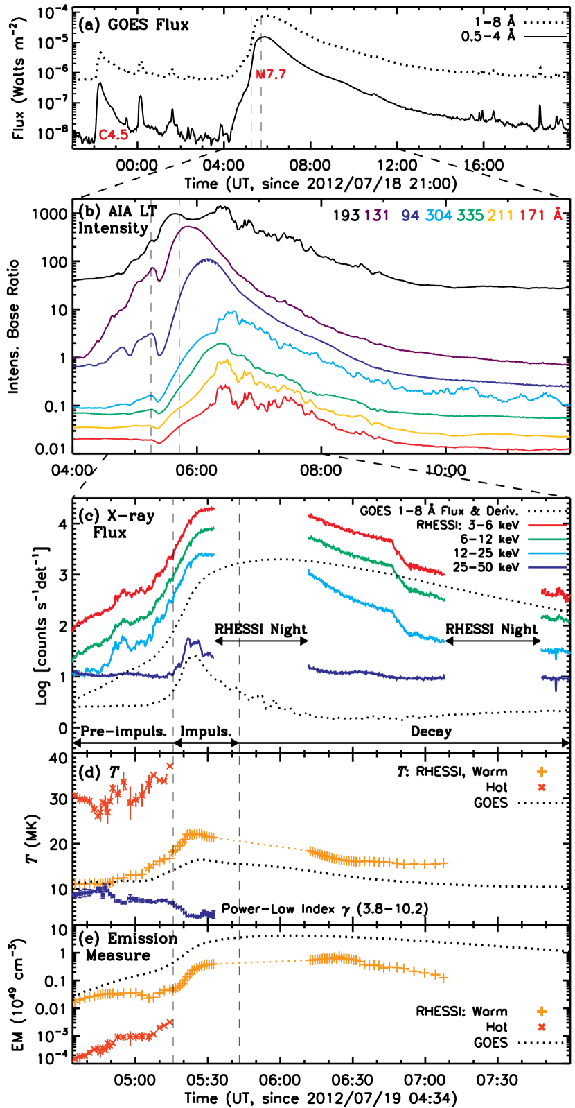
Figure 1.— History of X-ray and EUV flare emission. (a) GOES SXR fluxes showing the preceding C4.5 flare and the main M7.7 flare. (b) SDO/AIA intensity of the loop-top region (at projected height $h_{\rm ref}=60\arcsec$ on Cut 0, as shown in 13) normalized by its initial value (base ratio). Color-coded for AIA channels, the curves are vertically shifted to avoid overlap and arranged from the top to bottom approximately in the temporal order of their initial response to the flare (in progressively cooler channels). (c) RHESSI count rates in colored solid lines and GOES 1–8 Å flux and its time derivative in black dotted lines, arbitrarily shifted vertically. The two vertical dashed lines indicate the impulsive phase. (d) Temperature and (e) emission measure of the flare plasma inferred from RHESSI (orange/red) and GOES (black) spectral fits, together with the power-law index $\gamma$ of the nonthermal component shown in blue in (d).

1 shows the history of the flare emission. The GOES 1–8 Å flux peaks at 05:58 UT followed by a slow decay lasting almost one day. We define the interval of 05:16–05:43 UT as the impulsive phase, as marked by the two vertical dashed lines, which starts at the sudden rise of the RHESSI 25–50 keV flux and ends (during RHESSI night) when the time derivative of the GOES 1–8 Å flux drops to its level at the impulsive phase onset, assuming the Neupert (1968) effect at work. We call the intervals before and after the impulsive phase the pre-impulsive and decay phases. RHESSI has good coverage except for the late impulsive and early decay phases.

2 and its associated Movie A show AIA images of the event. An earlier C4.5 flare occurred in the same location, peaking at 22:18 UT on 2012 July 18 (see 1(a)). This is a confined flare that produces a hot flux rope failing to erupt and cusp-shaped flare loops underneath it (2(a)). This configuration then gradually evolves for hours and finally becomes unstable, initiating the later, eruptive M7.7 flare, when the flux rope is expelled as a fast CME of $>$$1000\mathrm{\,km}\mathrm{\,s}^{-1}$. The flux rope in this two-stage eruption was reported by Patsourakos et al. (2013).

As shown in 2(i), the trailing edge of the CME displays a clear “V-shape”, which, together with the underlying “inverted-V shape” of cusp-like flare loops, suggests two Y-type null points with a vertical current sheet formed in between, as predicted in the classical picture of eruptive flares (Carmichael, 1964; Sturrock, 1966; Hirayama, 1974; Kopp & Pneuman, 1976). Not predicted in that picture is the initial upward growth of the cusp followed by its rapid downward shrinkage around the early impulsive phase, prior to another, expected upward growth through the decay phase in a commonly observed candle-flame shape (Figures 2(a)–(l)). The initial growth and shrinkage are accompanied by the gradual rise and impulsive eruption of the overlying flux rope, respectively. Equally interesting are high-speed bi-directional outflows involving upward-moving plasmoids and downward-contracting pointed cusps (2, bottom; 5). We examine these and related features observed by RHESSI and AIA in next several sections.

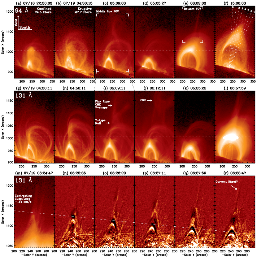
Figure 2.— AIA images of the event, rotated to the solar west up. Top: 94 Å image sequence of the earlier C4.5 flare and the M7.7 flare under study (see the associated online Movie A for composite 94 (red) and 335 Å (green) images). The brackets in (c) and (e) mark the enlarged fields of view (FOV) of the middle and bottom panels, respectively. The numbered dotted lines in (f) mark the cuts for obtaining space-time plots presented in this paper. Middle: Detailed 131 Å image sequence showing the upward growth of the flare cusp, followed by its rapid shrinkage around the early impulsive phase. The horizontal dotted line marks the highest position of the early cusp. Bottom: 131 Å image sequence showing an example of pointed cusps contracting from a ray-like structure, presumably a reconnecting current sheet (see the associated Movie B). The first panel is an original image and the rest are running difference images. The slanted dashed line indicates an average contraction velocity of $-151\mathrm{\,km}\mathrm{\,s}^{-1}$.

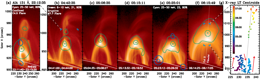
Figure 3.— (a)–(f) Evolution of RHESSI 6–10 keV sources (green contours at 31% and 90% of the maximum) overlaid on concurrent AIA 131 Å images (see the accompanying Movie). The blue contours show 25–50 keV emission, for both the C4.5 and M7.7 flares, at the footpoint(s) and the Masuda-type coronal source $20\arcsec$ above the SXR and EUV loops. (g) Color-coded temporal migration of the 6–10 keV loop-top centroid as marked by the plus sign on the left. The red arrows indicate an initial ascent followed by a descent and then another ascent. The dotted line marks the fiducial line (Cut 0) for obtaining projected heights shown in 4. The first and last panels are enlarged from the bracketed regions shown in their adjacent panels.

3. Overall X-ray and EUV Source Motions

We first follow the evolution of the morphologies and positions of overall X-ray and EUV sources.

3.1. X-ray Source Morphology

We reconstructed RHESSI X-ray images in energy bands from 3 to 50 keV using the CLEAN algorithm and detectors 3–9. Depending on the count rate, we chose variable integration time ranging from 20 s during the impulsive phase to 4 minutes during the decay phase.

3 and its accompanying Movie show examples of RHESSI contours overlaid on AIA images. There is a persistent loop-top source at 6–10 keV (green) near the apex of the cusp-shaped EUV loops. Accompanying the evolution of the EUV loops mentioned above, this loop-top source undergoes a gradual ascent followed by a descent and then another ascent. This can be best seen in the last panel showing the temporal migration of the emission centroid obtained from a contour at 70% of the maximum of each image. Early descents of loop-top X-ray sources have been recognized (e.g., Sui et al., 2004), but this is the first time that an evident preceding ascent is observed.

Early in the event there is an additional, weaker coronal X-ray source (panel (b)) located in the lower portion of the overlying flux rope. It later falls below detection with the eruption of the flux rope. During the impulsive phase (panel (e)) at higher energies (25–50 keV), there are double footpoint sources and a Masuda-type (Masuda et al., 1994; Nitta et al., 2010, e.g.,) coronal source located $20\arcsec=15\mathrm{\,Mm}$ above the SXR (6–10 keV) loop-top. This separation is twice that of the Masuda case.

The earlier C4.5 flare (panel (a)), though more compact, exhibits surprisingly similar emission, including the additional X-ray source within the flux rope and the Masuda-type hard X-ray (HXR) source. This suggests that the end state of the first, confined flare of a failed eruption serves as the initial state of the second, eruptive flare, making them homologous flares. Note that the weaker, southern footpoint emission is (partially) occulted by the limb, especially for the first flare.

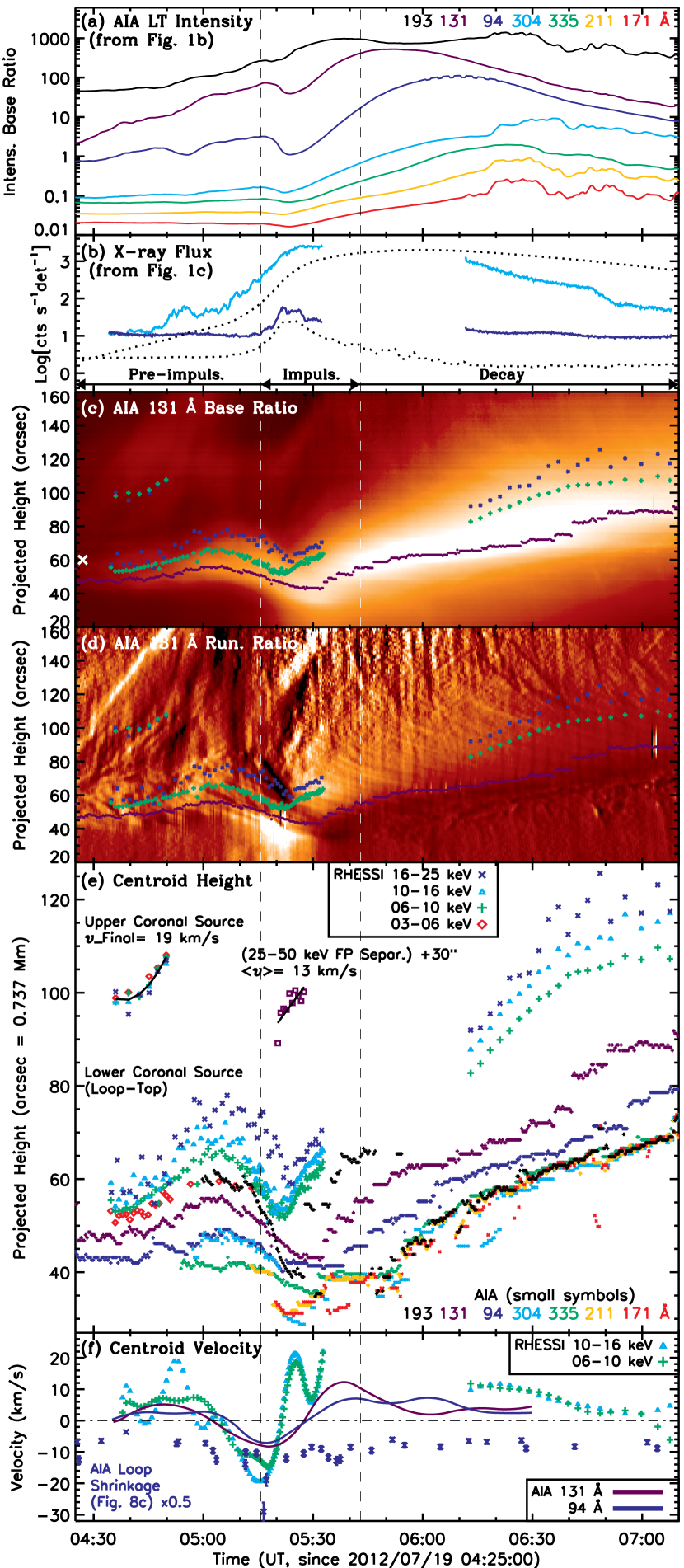
Figure 4.— X-ray and EUV source motions. (a) and (b) Subsets of light curves from Figures 1(b) and (c). (c) and (d) Base and running ratio space-time plots of the AIA 131 Å channel from Cut 0, overlaid with selected centroid positions from (e). (e) Projected heights of the emission centroids of the upper and lower coronal sources from RHESSI (large symbols, greater heights) and of the loop-top peaks from AIA (small symbols, lower heights). Also shown is the 25–50 keV footpoint separation (purple squares) shifted upward by $30\arcsec$. (f) Velocity of centroids from spline fits to selected channels in (e). The blue symbols are the initial velocities of individual but rescaled by a factor of 0.5.

3.2. X-ray and EUV Height-time History

To track various moving features, we placed eight cuts of $10\arcsec$ wide centered on the limb, as shown in 2(f). Cut 0 is positioned along the presumable current sheet between the initial flare cusp and erupting flux rope, and is used as the fiducial line for obtaining projected heights up to $\sim$08:00 UT. Subsequent cuts are evenly spaced by $3^{\circ}$ to capture the cusp at different stages as it gradual turns toward the south. For each cut, we averaged pixels of an AIA image sequence within it in the perpendicular direction to obtain a space-time plot.

4(c) shows, for example, a base-ratio (i.e., normalized by the initial intensity profile) space-time plot from Cut 0 at 131 Å. It shows the eruption of the flux rope and the three-stage development (upward, downward, and upward again) of the underlying flare cusp. The peak emission at each time, marked by the small purple symbols, evidently exhibits this motion. Space-time plots of other AIA channels are shown in 13 and described in Appendix A.

4(e) shows the height-time history of the loop-top emission centroids in four RHESSI X-ray bands from 3 to 25 keV and in all AIA EUV channels. (From now on, we refer to both X-ray centroids and EUV peaks as centroids.) We find that all loop-top centroids follow the same three-stage motions. The AIA 131 and 94 Å channels best exhibit this trend continuously, while in cooler channels, especially 211 and 171 Å, the initial ascent and subsequent descent become obscure. Note that the 3–6 keV centroid (red diamonds) cannot be identified since the impulsive phase because the RHESSI thin attenuator moves in and raises the energy threshold to 6 keV.

Table 2Projected Heights and Velocities of RHESSI and AIA Loop-top (LT) Centroids

Channels

Height (arcsec=0.737 Mm)/Time (UT)

Velocity ($\mathrm{\,km}\mathrm{\,s}^{-1}$)/Time (UT)

Initial

Max

Min

Descent %

Initial Ascent

Descent

2nd Ascent

($\sim$04:35)

Mean

Max

–6:00

6:00–7:00

7:00–8:00

RHESSI

16–25 keV

59″

77″/05:07

60″/05:24

22%

8.9

$-12$

$-23$/05:20

14

12

1.5

10–16 keV

55″

69″/05:06

54″/05:21

22%

7.1

$-15$

$-19$/05:15

14

10

3.6

6–10 keV

53″

66″/05:05

52″/05:22

21%

6.0

$-11$

$-15$/05:18

13

9.6

2.1

3–6 keV

52″

60″/05:04

…

…

4.1

…

…

…

…

…

AIA

193 Å

…

61″/05:03

35″/05:31

(43%)

…

$-13$

$-20$/05:19

…

4.9

3.0

131 Å

47″

56″/05:02

43″/05:30

23%

4.3

$-5.9$

$-8.3$/05:18

11

3.6

2.6

94 Å

43″

49″/05:06

41″/05:29

16%

2.5

$-4.7$

$-7.1$/05:17

5.9

3.2

2.6

304 Å

…

48″/05:04

29″/05:27

(40%)

…

$-5.1$

…

4.6

4.1

2.4

335 Å

…

41″/05:07

36″/05:29

12%

…

$-3.9$

…

4.1

3.5

3.2

211 Å

…

…

31″/05:23

…

…

$-6.9$

…

5.0

4.3

3.2

171 Å

…

…

31″/05:24

…

…

$-6.0$

…

5.6

5.0

3.5

We also notice a clear energy dispersion that the loop-top emissions at higher temperatures or photon energies are located at greater heights, with all X-ray centroids situated above EUV centroids. For example, at its greatest height prior to the impulsive phase, the 16–25 keV centroid is $35\arcsec=26\mathrm{\,Mm}$ above its 335 Å counterpart. This energy dispersion is consistent with previous observations (e.g., Veronig et al., 2006) and in line with the expected picture that higher loops are newly energized and thus are hotter and/or host nonthermal electrons of harder spectra, while lower loops are previously energized and have undergone cooling. We suggest that the so-called above-the-loop-top Masuda-type sources, including the 25–50 keV coronal source in 3(d), could be extreme cases of this general trend.

In Table 2, we list the initial heights of X-ray and EUV loop-top centroids around 04:35 UT, together with the maximum and minimum heights during their descents and the percentage height reductions. In general, the above noted energy dispersion persists and the 10–20% descents are in agreement with earlier reports (Veronig et al., 2006). An exception is the 193 and 304 Å channels because of their response to both hot and cool emissions (see Appendix A). There is a weak trend that higher energy X-ray descents start (at the maximum heights) later, but still within 5 minutes during 05:02–05:07 UT, and X-ray descents end (at the minimum heights) earlier than EUV descents by up to 10 minutes.

We measured the average velocities of the loop-top centroids by fitting a piecewise linear function to the height-time data during their initial ascent, subsequent descent, and second ascent stages. As listed on the right hand side of Table 2, the result shows a general trend of higher velocities at higher energies. The X-ray descents of $-11$ to $-15\mathrm{\,km}\mathrm{\,s}^{-1}$ are about twice faster than the EUV descents except for 193 Å because of its dual temperature response. There is also a gradual decrease in velocity with time during the second ascent stage through the decay phase. These trends generally agree with previous observations (Liu et al., 2004; Veronig et al., 2006).

To follow the temporal variations of the loop-top velocities, we took time derivatives of spline fits to the centroid heights of selected channels. The resulting velocities vs. time are shown in 4(c) for the 6–10 & 10–16 keV and 131 & 94 Å channels. The outstanding feature is that the maximum descent velocities (also tabulated in Table 2) in the range of $-7$ to $-23\mathrm{\,km}\mathrm{\,s}^{-1}$ are all attained during 05:15–05:20 UT, near the onset of the impulsive phase at 05:16 UT marked by a vertical dashed line. This time is delayed from the initial descent by about 10 minutes. This indicates that the loop-top descent velocity, rather than its height, is more intimately correlated with the energy release rate.

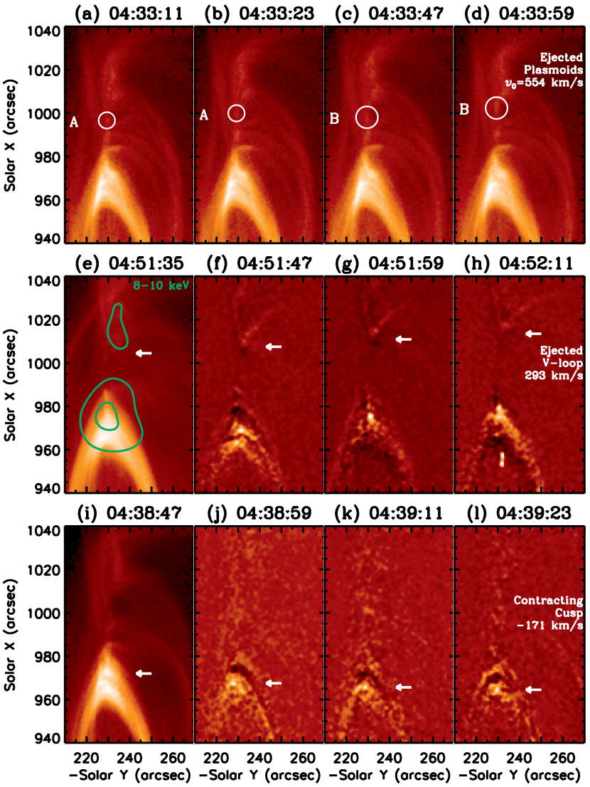
Figure 5.— AIA 131 Å images (see the accompanying Movie) showing upward moving blobs (top, labeled A and B) and V-shapes (middle) and downward contracting cusps (bottom). Their space-time fits are shown in 7(a). The green contours show two distinct 8-10 keV RHESSI sources from 10(c). The first row and column are original images and the rest are running difference images.

We also show in 4(e) the centroid heights of the upper coronal X-ray source located in the lower portion of the flux rope. A parabolic fit indicates a final velocity of $19\mathrm{\,km}\mathrm{\,s}^{-1}$ at 04:50 UT, comparable to or slower than those in other events (Liu et al., 2008, 2009c; Sui & Holman, 2003). It is also 50% slower than the middle portion of the then accelerating flux rope, as indicated by the parabolic fit in 13(e), which reaches $153\pm 3\mathrm{\,km}\mathrm{\,s}^{-1}$ later at 05:07 UT near the edge of AIA’s FOV.

The conjugate footpoints at 25–50 keV during the impulsive phase move away from each other at an average velocity of $13\mathrm{\,km}\mathrm{\,s}^{-1}$ (see 4(e)), almost identical to the velocity of the simultaneous loop-top ascent (see Table 2). This is consistent with previous observations (Liu et al., 2004) and the classical picture of eruptive flares during the arcade growth phase.

4. Bi-directional Plasma Outflows

We now turn our attention to the bi-directional plasma outflows observed by AIA. As shown in 5 and its accompanying Movie, emission features move both upward and downward from above the cusp-shaped flare loops. The upward outflows, observed only when the flux rope rises toward its eruption, are mainly bright blobs (interpreted as plasmoids, top row), while the downward outflows are primarily in the form of retracting cusp-shaped loops (bottom row) observed throughout the event well into the decay phase. Among the downward retracting loops, those seen at low altitudes tend to have lower speeds ($\lesssim$$60\mathrm{\,km}\mathrm{\,s}^{-1}$) and gradually decelerate when approaching and piling up onto the apex of the flare arcade, while those originating from high altitudes tend to have higher speeds ($\gtrsim$$100\mathrm{\,km}\mathrm{\,s}^{-1}$) and decelerate more rapidly. According to these observational distinctions, we call the former slow loop shrinkages and the latter fast loop contractions, although they might share a common physical origin as discussed in Section 6. The former are likely analogous to shrinkages observed at SXR and other wavelengths (Švestka et al., 1987), while the latter, especially those occurring after the flare arcade has formed, are likely so-called supra-arcade downflow loops (Savage & McKenzie, 2011).

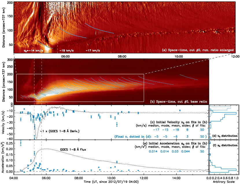
Figure 6.— Kinematic measurements of slow loop shrinkages. (a) Running ratio space-time plot enlarged for the boxed region in (b), overlaid with examples of fits to shrinkage tracks labeled with their initial velocities. (b) Base ratio 131 Å space-time plot from Cut 0 overlaid with all 50 fits performed. (c) Initial velocities $v_{0}$ of the fitted tracks in (b) as a function of time. (d) Histograms of $v_{0}$ (solid) and the final velocity $v_{f}$ (dotted) measured at the end of each track, with their statistical properties (median, mode, mean, standard deviation, and total number of fits) listed in (c). (e) and (f) same as (c) and (d), but for the initial acceleration $a_{0}$. The black dotted lines in (c) and (e) are the time derivative (inverted) and original GOES 1–8 Å flux. The two vertical dashed lines mark the impulsive phase.

To track these moving features, we obtained space-time plots from the cuts defined in 2(f) using the 131 Å channel because it provides the best coverage of these features. We then applied running ratio, namely, dividing the intensity profile at each time by its previous neighbor, which highlights moving features as intensity tracks (see, e.g., 4(d)). We exhaustively identified such tracks of more than $10\arcsec$ long corresponding to unique moving features. If one feature is captured by multiple cuts, we included only the most complete track. Following Warren et al. (2011), we fitted the projected height $h$ of each track by a function of time $t$,

$$h(t)=h_{0}+v_{T}t+a_{0}\tau^{2}(e^{-t/\tau}-1),$$ (1)

which gives the instantaneous velocity

$$v(t)=v_{T}-a_{0}\tau e^{-t/\tau},$$ (2)

and acceleration

$$a(t)=a_{0}e^{-t/\tau},$$ (3)

where $h_{0}$ and $a_{0}$ are the initial height and acceleration, $v_{T}$ is the terminal velocity, and $\tau$ is the $e$-folding decay time that characterizes the observed decreasing acceleration (or deceleration) with time. We present below the kinematics of the features categorized above and focus on their initial velocities $v_{0}=v_{T}-a_{0}\tau$ and accelerations $a_{0}$.

4.1. Slow Downward Loop Shrinkages

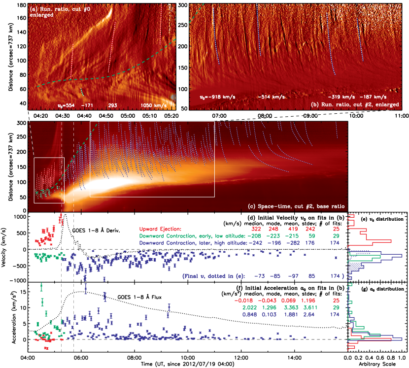
Figure 7.— Same as 6 but for fast upward plasmoid ejections and downward loop contractions. (a) and (b) Running ratio space-time plots obtained from Cuts 0 and 2, enlarged for the two boxed regions in (c). Overlaid with examples of color-coded fits, (a) shows simultaneous upward ejections (red dotted) and downward contractions of early, low-lying loops (green dotted), and (b) shows downward contractions of later, high-lying loops (blue dotted) from well above the flare arcade. Example images corresponding to the fits in (a) and (b) are shown in Figures 5 and 2 (bottom), respectively. (c) Base ratio 131 Å space-time plot from Cut 2 overlaid with all fits to these identified features. The thick green dashed line is a spline fit to the initial heights of bi-directional outflows, as an estimate to the position of reconnection. (d)–(g) Initial velocities $v_{0}$ and accelerations $a_{0}$ of the color-coded fits in (c) as a function of time, together with their histograms on the right. The blue dotted line in (e) is for the final velocities of the late, high-lying loop contractions. The short, vertical stripes in (a) with a periodicity of $\sim$1 minute between 04:45–05:15 UT are possibly due to quasi-periodic flare pulsations (Nakariakov & Melnikov, 2009), not to be confused with the tracks of steep slopes of plasma outflows.

6 shows kinematic measurements of the slow loop shrinkages. These loops traverse a hot (up to $T\sim 30\mathrm{\,MK}$; see 11) loop-top region, which is bright only in the hottest channels of 193, 131, and 94 Å, and descend toward the apex of the flare arcade seen in cooler channels, where they fade below detection (see 13). They generally start at a low velocity with a median of $-17\mathrm{\,km}\mathrm{\,s}^{-1}$ ($+/-$ for upward/downward) and decelerate to typically $-5\mathrm{\,km}\mathrm{\,s}^{-1}$ within 0.5–2.5 h. Their median initial deceleration is $0.014\mathrm{\,km}\mathrm{\,s}^{-2}$.

Such shrinkages are persistent throughout the flare, not only during the decay phase when the overall loop-top emission develops upward as previously observed (Forbes & Acton, 1996), but also during the pre-impulsive and impulsive phases when the loop-top undergoes its initial ascent and subsequent descent. 50 shrinkages are identified during 04:00–16:00 UT with an average occurrence rate of once per 7.7 minutes up to 10:00 UT but more frequent around the impulsive phase (6(b)).

Regardless of the direction of motion of the loop-top emission, the initial height of loop shrinkage generally increases with time. The initial velocity $v_{0}$ exhibits more variability, as shown in 6(c), and appears to be positively correlated with the flare energy release rate indicated by the time derivative of the GOES flux (black dotted line). In particular, near the onset of the impulsive phase at 05:16 UT (vertical dashed line), $v_{0}$ increases rapidly and reaches a maximum of $-58\mathrm{\,km}\mathrm{\,s}^{-1}$. There is a similar temporal correlation with the initial deceleration $a_{0}$ (panel (d)) that also generally correlates with $v_{0}$.

4.2. Fast Downward Loop Contractions

7 shows, in the same form as 6, kinematic measurements of fast downward loop contractions as well as upward plasmoid ejections that will be examined in Section 4.3. We color-code fits to tracks of different categories: upward ejections in red and downward contractions in cooler colors. For the latter, we use green for early contractions that occur simultaneously with upward ejections and originate from lower heights $h<100\arcsec$, and blue for later contractions that occur without observed upward counterparts (possibly out of AIA’s FOV, after the flux rope has erupted) and originate from greater heights $h>100\arcsec$. We identified 29 green tracks and 174 blue tracks during 04:00–16:00 UT.

As shown in 7(c), the fast downward contractions, especially those later blue-colored ones, start well above the hot loop-top region and travel into it with deceleration for some distance before fading below detection. Their final heights are generally above the original heights of slow loop shrinkages (see 6(b)).

In original AIA images, the fast contracting features are usually bright, cusp-shaped loops (see 2, bottom), but occasionally dark, tadpole-like voids (McKenzie & Hudson, 1999; Innes et al., 2003; Cassak & Drake, 2013). In running ratio space-time plots (7, top), the former each produce a bright track followed by a recovering dark track, while the latter produce tracks of reversed order. We treat them all as contracting loops and do not distinguish their differences that are beyond our scope.

Table 3Kinematic Statistics of Bi-directional Outflows

Features	Interval(a)	Initial Velocity ($\mathrm{\,km}\mathrm{\,s}^{-1}$)						Final Velocity ($\mathrm{\,km}\mathrm{\,s}^{-1}$)						Initial Acceleration ($\mathrm{\,km}\mathrm{\,s}^{-2}$)
(# of Fits)	(minutes)	Med.	Mod.	$\sigma$	Max/Time	Min		Med.	Mod.	$\sigma$	Max/Time	Min		Med.	Mod.	$\sigma$	Max/Time	Min
Ejected Plasmoids (25)	2.4	$322$	$248$	$242$	$1050$/05:15	$121$		$343$	$320$	$250$	$1070$/05:13	$70$		$-0.018$	$-0.043$	$1.2$	$2.89$/05:12	$-2.84$
Shrinking Loops (50)	7.7	$-17$	$-15$	$8$	$-58$/05:16	$-7$		$-5$	$-5$	$3$	$-18$/04:26	$-2$		$0.014$	$0.014$	$0.044$	$0.252$/04:26	$-0.008$
Contracting Cups:
Early, Low Altit.(29)	2.2	$-208$	$-231$	$59$	$-351$/04:30	$-110$		$-89$	$-68$	$58$	$-226$/04:30	$-26$		$2.022$	$1.30$	$3.61$	$16.9$/04:30	$0.096$
Late, High Altit.(174)	2.0	$-242$	$-158$	$176$	$-918$/06:52	$-34$		$-73$	$-113$	$85$	$-553$/05:32	$-1$		$0.848$	$0.103$	$2.64$	$15.9$/06:10	$-0.297$

As shown in 7(c), the early, green-colored contractions have short ranges of $10\arcsec$–$20\arcsec$, because of the compactness of the flare at this time, while the later, blue-colored contractions travel great distances up to $200\arcsec=150\mathrm{\,Mm}$. However, their statistical medians, modes, and means of the initial velocities are quite similar within $200$–$300\mathrm{\,km}\mathrm{\,s}^{-1}$ (Figures 7(d) and (e); Table 3), suggestive of a common origin of these contractions possibly as reconnection outflows. The initial decelerations of the early contractions are, on the other hand, about twice higher than those of the later ones, with a median of 2.022 vs. $0.848\mathrm{\,km}\mathrm{\,s}^{-2}$ (Figures 7(f) and (g)).

The later, high-altitude contractions have a mode velocity $-158\mathrm{\,km}\mathrm{\,s}^{-1}$ that is similar to the median velocity $-150\mathrm{\,km}\mathrm{\,s}^{-1}$ of supra-arcade downflows (Savage & McKenzie, 2011; Warren et al., 2011). However, their median and mean velocities, $-242$ and $-282\mathrm{\,km}\mathrm{\,s}^{-1}$, are nearly twice greater. This is due to the high velocity tail with 36 out of 174 or 21% contractions being faster than $-400\mathrm{\,km}\mathrm{\,s}^{-1}$ (hatched area in 7(e)), reaching a maximum of $-918\mathrm{\,km}\mathrm{\,s}^{-1}$. We ascribe this difference to AIA’s improved capabilities that allow us to detect such contractions in their early stages when their velocities are high and emissions are weak.

The initial velocities and decelerations of the earlier and later fast contractions, when taken together, generally increase with time up to $\sim$06:10 UT and then decrease. This maximum time is delayed by almost 1 h from that of the slow loop shrinkages and the onset of the HXR burst represented by the GOES flux derivative shown in 6(c). The temporal variations here seem to be more closely correlated with the GOES flux itself. The late-phase decreases of the initial velocities and decelerations are physically reasonable as energy release subsides, but there is an observational bias for those tracks starting at the edge of AIA’s FOV which may have decelerated before they are first detected.

8 shows the distributions of fractional height reductions of the downward loop shrinkages and contractions, defined as $(h_{0}-h_{f})/h_{0}$, where $h_{0}$ and $h_{f}$ are the initial and final projected heights. The slow shrinkages (light blue) and later, high-altitude fast contractions (blue) have similar distributions with medians of 0.3 and 0.26, respectively, which are comparable to those observed in SXRs (Forbes & Acton, 1996; Reeves et al., 2008) and predicted theoretically (Lin, 2004). The early, low-altitude fast contractions (green) have a median of twice smaller, but comparable to the 10–20% descent of the overall loop-top emission (Table 2). Meanwhile, the later fast contractions have a sizable fraction of 16% (27 out of 174) with height reductions more than 0.4 (up to 0.7), which is larger than predicted. Note that these observed values are lower limits, because loops, especially those detected at the edge of AIA’s FOV, could continue contraction before and after their observed intervals when their emission remains below detection.

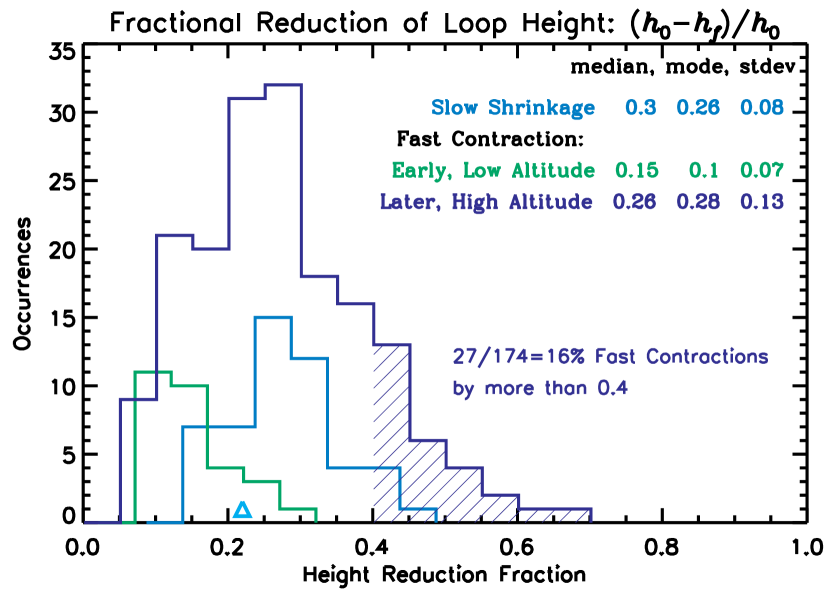
Figure 8.— Histograms of fractional height reductions of slow shrinkages (light blue) and early, low-altitude (green) and later, high-altitude (blue) fast contractions. The hatched area indicates 16% of the later fast contractions with reductions greater than 0.4. The cyan triangle marks the descent fraction of the 10–16 keV loop-top from Table 2.

4.3. Fast Upward Plasmoid Ejections

As shown in 7, upward plasmoid ejections appear as steep, elongated tracks (red fits). Compared with the downward loop contractions (green fits) at the same time, they travel greater distances ($20\arcsec$–$80\arcsec$ vs. $10\arcsec$–$20\arcsec$), with larger initial velocities (median: 322 vs. $-208\mathrm{\,km}\mathrm{\,s}^{-1}$) but smaller decelerations (median: $-0.018$ vs. $2.022\mathrm{\,km}\mathrm{\,s}^{-2}$). (The opposite signs of the acceleration and velocity here indicate deceleration.) Some upward ejections even experience acceleration. Such differences, especially the ratio of their median velocities of $208/322=2/3$, are consistent with previous observations and simulations of oppositely directed reconnection outflows (Takasao et al., 2012; Bárta et al., 2008; Shen et al., 2011; Murphy et al., 2012; Karpen et al., 2012). These differences are likely due to different environments: the upflow runs into a region of (partially) open field lines with low plasma density, while the downflow impinges on high density, closed flare loops that can cause strong deceleration.

The starting heights of these upward ejections and their downward counterparts (7 (c)) both increase with time. This suggests an upward development of the reconnection site situated between the opposite outflows (e.g., Shen et al., 2011). We estimated the height of the reconnection site from a spline fit, shown as the green dashed line in Figures 7(a)–(c), to the initial heights of the bi-directional fast outflows. Its initial velocity of a few $\mathrm{\,km}\mathrm{\,s}^{-1}$ is similar to that of the initial loop-top ascent, suggesting the upward development of reconnection being its underlying mechanism. This estimated reconnection site leaves the AIA FOV at about 06:40 UT.

During 04:15–05:25 UT, we identified 25 upward ejections (red) and 29 downward, early fast contractions (green), at average occurrence rates of once every 2.4 and 2.2 minutes, respectively. These rates are comparable to that of the later fast contractions (blue, up to 10:00 UT) of once every 2.0 minutes and to those in MHD simulations (Bárta et al., 2008). The persistence throughout the entire flare of such contractions also agrees with the statistical result from Yohkoh (Khan et al., 2007).

The initial velocity of upward ejections, as shown in 7(d), increases with time and seems to be correlated with the height of the overlying flux rope as it evolves into eruption. In particular, there is a rapid velocity increase at the onset of the impulsive phase, reaching $1050\mathrm{\,km}\mathrm{\,s}^{-1}$. This aspect of this event is independently studied by R. Liu (2013).

5. Spatial Distribution of Energy and Temperature Dependent Emission

5.1. RHESSI X-ray Spectra

To infer the overall properties of nonthermal particles and thermal plasma, we analyzed spatially integrated RHESSI spectra of individual detectors following the procedures detailed in Liu et al. (2008) and Milligan & Dennis (2009).

9 shows example spectra in three phases of the flare. (1) During the pre-impulsive phase (04:59:00–05:01:32 UT), we fitted the spectrum with two isothermal functions combined: a warm component (red dotted) of temperature $T=13\mathrm{\,MK}$ and emission measure ${\rm EM}=0.37\times 10^{48}\mathrm{\,cm}^{-3}$ plus a hot component (green dotted) of $30\mathrm{\,MK}$ (also called super-hot, Caspi & Lin, 2010) and a 40 times smaller EM. If we were to replace the hot component with a power-law $\propto E^{-\gamma}$, we would have a steep slope of $\gamma=7.6$. (2) During the impulsive phase (05:25–05:26 UT), we used an isothermal ($T=22\mathrm{\,MK}$, ${\rm EM}=2.8\times 10^{48}\mathrm{\,cm}^{-3}$) plus power-law (blue dotted, $\gamma=3.8$) model. (3) During the decay phase, the data can be fitted with one isothermal function of a slightly reduced temperature of $18\mathrm{\,MK}$ but twice higher EM of $5.5\times 10^{48}\mathrm{\,cm}^{-3}$. Note that at $E$$>$25 keV, the power law in the impulsive phase is more than an order of magnitude higher than the thermal component. This indicates that the 25–50 keV Masuda-type loop-top source shown in 3 is primarily nonthermal and likely a particle acceleration region itself (e.g., Liu et al., 2008; Krucker et al., 2010).

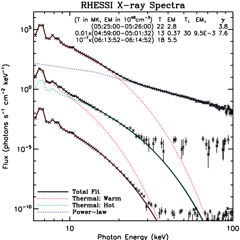
Figure 9.— RHESSI spectra at three selected times before, during, and after the impulsive phase. The lower two spectra are vertically shifted by decades to avoid overlap. Colored dotted lines are isothermal and power-law fits whose parameters are listed on the top. The black solid lines are the total fits.

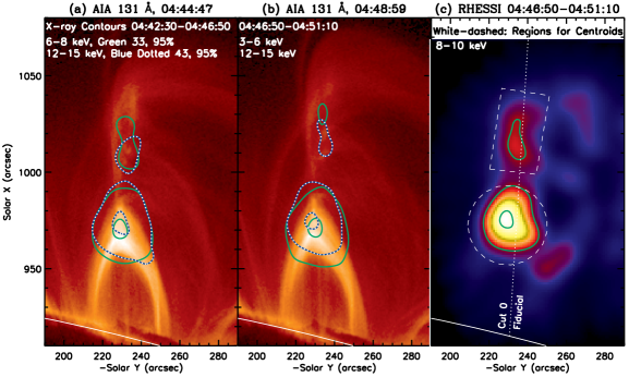
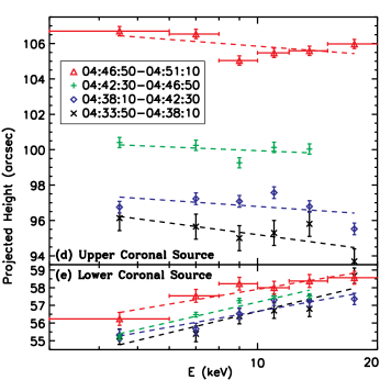
Figure 10.— Energy dependence of the double coronal X-ray sources likely located in the oppositely directed reconnection outflows. (a) and (b) RHESSI contours overlaid on AIA 131 Å images. The higher energy sources (blue dotted contours at 43% and 95% of the image maximum) are closer toward one another than the lower energy sources (green contours). (c) Contoured 6–8 keV image at the time of (b). (d) and (e) Projected heights along the fiducial Cut 0 of the centroids of the two sources enclosed by the white dashed lines in (c). The result is color-coded for four consecutive times overlaid with linear fits in dashed line. The red horizontal error bars indicate energy bins.

We applied such spectral fits throughout the flare and the temporal variations of the fitting parameters are shown in Figures 1(d) and (e). In general, the warm thermal component is persistent in time, and both its $T$ and EM (orange plus signs) increase through the HXR burst followed by a more gradual decrease. A similar trend is present for the hot thermal component (red crosses) during the pre-impulsive phase. A thermal fit to GOES data gives a somewhat lower $T$ but higher EM (black dotted lines), because of its well-known preferential response to relatively cooler plasma. The power-law component (blue) displays a common hardening trend before the RHESSI night data gap.

5.2. Energy Dependence of Double Coronal Sources

In Section 3.2 we have examined the energy-dependent height distribution of the loop-top X-ray source (lower coronal source). Here we extend this analysis to the upper coronal source during the pre-impulsive phase and compare the two sources together.

As shown in Figures 10(a) and (b), the higher-energy emission (12–15 keV, blue contours) of the lower source is located at higher altitudes than lower-energy emission (3–8 keV, green contours), while the upper source has an opposite trend. That is, the two sources are closer to each other at higher energies, as can be better seen in panel (d) from the linear fits to their centroid heights as a function of logarithmic energy. This implies higher temperatures of the thermal plasma and/or harder spectra of the nonthermal particles within the inner regions. Similar RHESSI observations have been reported (Sui & Holman, 2003; Liu et al., 2008, 2009c) and interpreted as evidence of magnetic reconnection and associated energy release being located between the double coronal sources.

At the highest energies ($\gtrsim$10 keV), this trend seems to be reversed, especially for the upper source. In previous observations (e.g., Figure 4 in Liu et al. 2008), more obvious reversals occurred at slightly higher energies of 15–20 keV and were interpreted as a transition from the low-energy thermal regime to the high-energy nonthermal regime, in which greater stopping distances of higher energy electrons can cause higher energy bremsstrahlung X-rays being located farther away. We further suggest that this reversal may be an indication of the two X-ray sources being spatially separated, instead of merging together at the highest energies; so are the locations of primary heating and particle acceleration from magnetic reconnection. This is supported by the separate temperature peaks at the two sources as shown in Figures 11(a) and (h) and discussed in Section 5.3.

5.3. AIA Temperature Maps

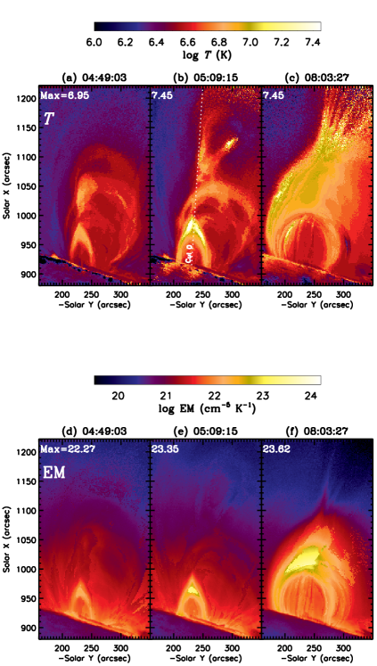
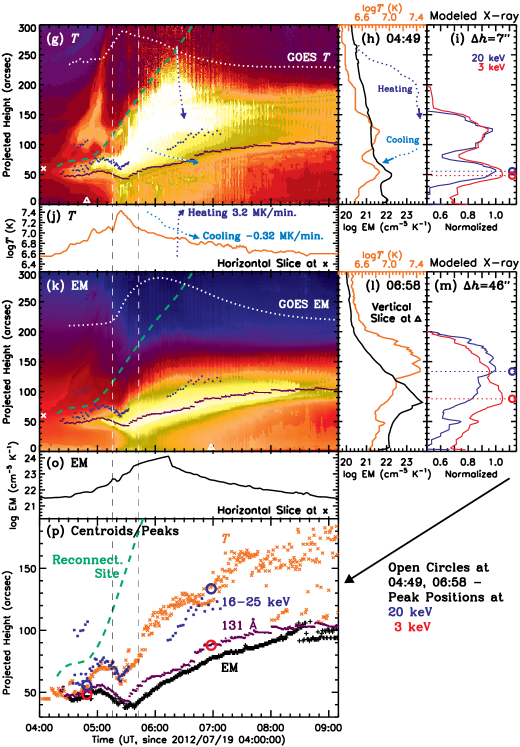
Figure 11.— Maps of temperature $T$ (a–c) and emission measure EM (d–f) inferred from AIA filter ratios at three selected times on logarithmic scales. (g) and (k) Space-time plots of $T$ and EM maps from Cut 0 as shown in (b). The white dotted lines are temperature and emission measure from GOES data as shown in Figures 1(d) and (e). The first side panels ((h) and (l)) on the right show the height distributions of $T$ (red, top scale) and EM (black, bottom scale) at the time marked by the triangle on the left. The second side panels ((i) and (m)) show the modeled corresponding thermal X-ray emission at two photon energies, 3 and 20 keV. The open circles mark the heights of the emission peaks that are also shown in (p). (j) and (o) Temporal profiles $T$ and EM, obtained from a horizontal slice of the corresponding space-time plots above at height $h_{\rm ref}=60\arcsec$ marked by the cross. The arrowed blue and light blue dotted lines in (g) are selected tracks of a fast contraction and slow shrinkage from Figures 7 and 6. The temperatures sampled by these tracks are shown as a function of time and distance in (j) and (h), respectively, indicating heating and cooling experienced by these loops as they travel. (p) Projected heights of the maxima of $T$ (orange) and EM (black) at each time in the corresponding space-time plots. Overlaid here and in the above space-time plots are the heights of the 16-25 keV (blue) and 131 Å (purple) loop-top centroids in small symbols from 4(e), and of the inferred reconnection site in green dashed line from 7(c). The vertical dashed lines mark the impulsive phase.

To infer the spatial distributions of temperature $T$ and emission measure (EM), we employed a forward-fitting algorithm using AIA filter ratios (Aschwanden et al. 2011; for a different approach, see Battaglia & Kontar 2012). This algorithm assumes a Gaussian differential emission measure that has a peak EM at temperature $T$. Such a model provides the simplest description of the EM weighted temperature distribution along the line of sight.

11 (left) shows examples of $T$ and EM maps. Early in the event at 04:49 UT, the highest temperature of $\log T=6.95$ or $T=8.9\mathrm{\,MK}$ is located in the rising flux rope and the underlying flare cusp, but EM is highly concentrated in the latter. The temperature then increases with time especially in the flare cusp, reaching $\log T=7.45$ or $T=28.2\mathrm{\,MK}$ at 05:09 UT, close to the 35 MK of the hot RHESSI component at this time (see 1(d), red crosses). In the decay phase, the highest temperatures are located in the outer layer of the flare arcade and the lower portion of the contracting cusps (ray-like features) above it. The EM in the latter is nearly four orders of magnitude lower than in the central arcade, similar to those of hot fans of rays observed by Yohkoh (Švestka et al., 1998). The considerable increase of EM and thus density in the flare loops from panel (d) to (e), prior to the impulsive phase, suggests chromospheric evaporation driven by thermal conduction (Liu et al., 2009b; Battaglia et al., 2009) or by Alfvén waves (Haerendel, 2009), rather than electron beam heating that may be important later in the presence of HXR footpoints.

To better follow the history of $T$ and EM, we obtained their space-time plots, as shown in Figures 11(g) and (k), from corresponding maps using Cut 0. We identified the maximum temperature and EM at each time and show their projected heights as orange and black symbols in panel (p). In general, both peaks follow the same upward-downward-upward motions as the loop-top emission centroids. The temperature peaks are near the RHESSI 16–25 keV centroids (blue), while the EM peaks are close to or slightly lower than the AIA 131 Å centroids (purple) at lower heights.

The peak offset of the temperature and EM can be better seen in their height distributions at selected times shown in Figures 11(h) and (l). It explains the observed energy dispersion of the X-ray loop-top centroids shown in 4(e) because of the exponential shape of thermal bremsstrahlung spectra (equation (4)). As shown by the green and red lines in the middle of 9, a higher temperature but lower EM produces a harder (shallower) spectrum of lower normalization that dominates at high energies, while a lower temperature but higher EM produces a softer (steeper) spectrum of higher normalization that dominates at low energies. The temperature peak being located above the EM peak thus shifts the higher energy X-rays toward greater heights. Otherwise, if the temperature and EM peaks are cospatial, they would dominate X-rays at all energies and there would be no separation of centroids with energy. We note in Figures 11(h) that the EM decreases more gradually near the flux rope. This may lead to the less pronounced energy dispersion of the upper coronal source there than the lower (loop-top) source (see 10).

As a proof of concept, we modeled the observed X-rays of energy $E$ with thermal bremsstrahlung radiation (Tandberg-Hanssen & Emslie, 1988, p. 114):

$$I_{\rm SXR}\propto({\rm EM}){\exp(-E/kT)\over E\sqrt{T}}g(E/kT),$$ (4)

where ${\rm EM}$ is the emission measure and $g(E/kT)=(kT/E)^{2/5}$ is the Gaunt factor. The resulting X-ray profiles at two selected times are shown in Figures 11(i) and (m) for the corresponding $T$ and EM profiles. As expected, the higher energy 20 keV emission (blue) is dominated by the temperature peak at a higher altitude, while the 3 keV emission (red) is dominated by the EM peak at a lower altitude. Their emission peaks, marked by open circles, differ in height by $\Delta h=7\arcsec$ and $46\arcsec$ for the two times. Their peak heights are repeated in panel (p) and are close to those of observed loop-top centroids.

As shown in Figures 11(g) and (p), the high temperature region and particularly the temperature peak are close to the X-ray loop-top centroids but always below the reconnection site (green dashed line). This indicates that primary plasma heating takes place in reconnection outflows. To illustrate this, we can follow a contracting loop and the temperature variation it senses as it travels away from the reconnection site. A selected track from 7(c) is shown here as the blue dotted arrow. The temperature history on its path, as shown in Figures 11(h) and (j), indicates rapid heating at an average rate of $3.2\mathrm{\,MK}\,{\rm min}^{-1}$ from 3.5 to 28 MK over 8 minutes and $\Delta h=90\mathrm{\,Mm}$. This example gives us a sense of the heating rate averaged along the line of sight, not necessarily of a specific loop.

Likewise, the track of a slow loop shrinkage at lower altitudes reveals cooling at an average rate of $-0.32\mathrm{\,MK}\,{\rm min}^{-1}$ from 25 to 7.9 MK within 54 minutes. The rate is $-1\mathrm{\,MK}\,{\rm min}^{-1}$ earlier during the impulsive phase in the 28–9 MK range and $-0.1\mathrm{\,MK}\,{\rm min}^{-1}$ later during 07:00–08:30 UT in the 14–7 MK range. These cooling rates are somewhat lower than previously found at even lower temperatures (Vršnak et al., 2006).

6. Conclusion

6.1. Summary

We have presented detailed EUV and X-ray observations of the 2012 July 19 M7.7 flare, focusing on the signatures of magnetic reconnection and associated energy release. We summarize our findings and discuss their implications as follows.

1. The V-shaped EUV emission on the trailing edge of the flux rope CME and the underlying, inverted V-shaped flare loops, both associated with distinct X-ray emission, suggest two oppositely oriented Y-type null points with a vertical current sheet formed in between (Figures 2 and 5).

2. Originating from the inferred magnetic reconnection site within the current sheet are bi-directional outflows in the forms of plasmoids and cusp-shaped loops. The upward ejections have a median initial velocity of $320\mathrm{\,km}\mathrm{\,s}^{-1}$ and a maximum of $1050\mathrm{\,km}\mathrm{\,s}^{-1}$, while the concurrent downward cusp contractions are $\sim$$2/3$ slower with a median of $-210\mathrm{\,km}\mathrm{\,s}^{-1}$. Even faster contractions up to $-920\mathrm{\,km}\mathrm{\,s}^{-1}$ occur after the flux rope eruption for another 10 h, and a sizable fraction of 21% of them have speeds $\geq$$400\mathrm{\,km}\mathrm{\,s}^{-1}$, twice faster than previously reported (Savage & McKenzie, 2011). Such high velocities are comparable to expected coronal Alfvén speeds of $\sim$$1000\mathrm{\,km}\mathrm{\,s}^{-1}$ and sound speeds of 520–$910\mathrm{\,km}\mathrm{\,s}^{-1}$ for a 10–30 MK flaring plasma. At lower altitudes, flare loops persistently shrink at typical initial velocity of $-17\mathrm{\,km}\mathrm{\,s}^{-1}$ and gradually decelerate to about $-5\mathrm{\,km}\mathrm{\,s}^{-1}$ within 0.5–2.5 h. They are all evidence of reconnection outflows during different stages (Figures 6 and 7).

3. The double coronal X-ray sources are spatially separated and located in the regions of bi-directional plasma outflows. The highest temperature is found near the loop-top X-ray source well below the reconnection site. This suggests that primary plasma heating and particle acceleration take place in the reconnection outflow regions (Holman, 2012), rather than at the reconnection site itself. Models with this ingredient were proposed long ago (e.g., Forbes & Priest, 1983), but solid observational evidence as presented here has been lacking (Figures 10 and 11).

4. An energy dispersion is present in the loop-top position with higher-energy X-ray and hotter EUV emission located at greater heights over a large range of $\Delta h\geq 26\mathrm{\,Mm}$. The 25–50 keV nonthermal emission lies $15\mathrm{\,Mm}$ (twice that of the Masuda flare) above the 6–10 keV thermal emission. This agrees with the expected trend of softer electron spectra in the nonthermal regime and lower temperatures in the thermal regime being associated with earlier energized loops, which are located further below the primary locus of energy release. The upper coronal X-ray source has an opposite trend because it is located in the oppositely directed reconnection outflow (Figures 3, 4, and 10).

5. Prior to the recently recognized descent followed by a continuous ascent, the overall loop-top emission experiences an initial ascent for nearly an hour. This is the first time that such motions, including the descent, are observed simultaneously from EUV to HXRs covering a wide range of temperatures of 1–30 MK. The transition from ascent to descent coincides with the rapid acceleration of the flux rope CME. The loop-top descends at $\sim$$10\mathrm{\,km}\mathrm{\,s}^{-1}$, about 50% slower in EUV than in X-ray (4).

6. The flare impulsive phase starts when a rapid velocity increases occur for the overall loop-top descent, the individual loop shrinkages, and the upward plasmoid ejections. This is delayed by 10 minutes from the initial loop-top descent, implying that the energy release rate is more intimately correlated with these velocities than the loop-top position (4).

6.2. Proposed Physical Picture

We propose the following physical picture to tie together the observations. The major points, including the location of particle acceleration and the three-stage (up-down-up) motion of the loop-top X-ray source, are sketched in 12.

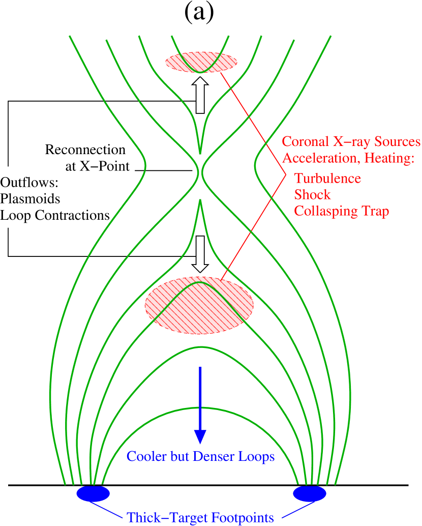
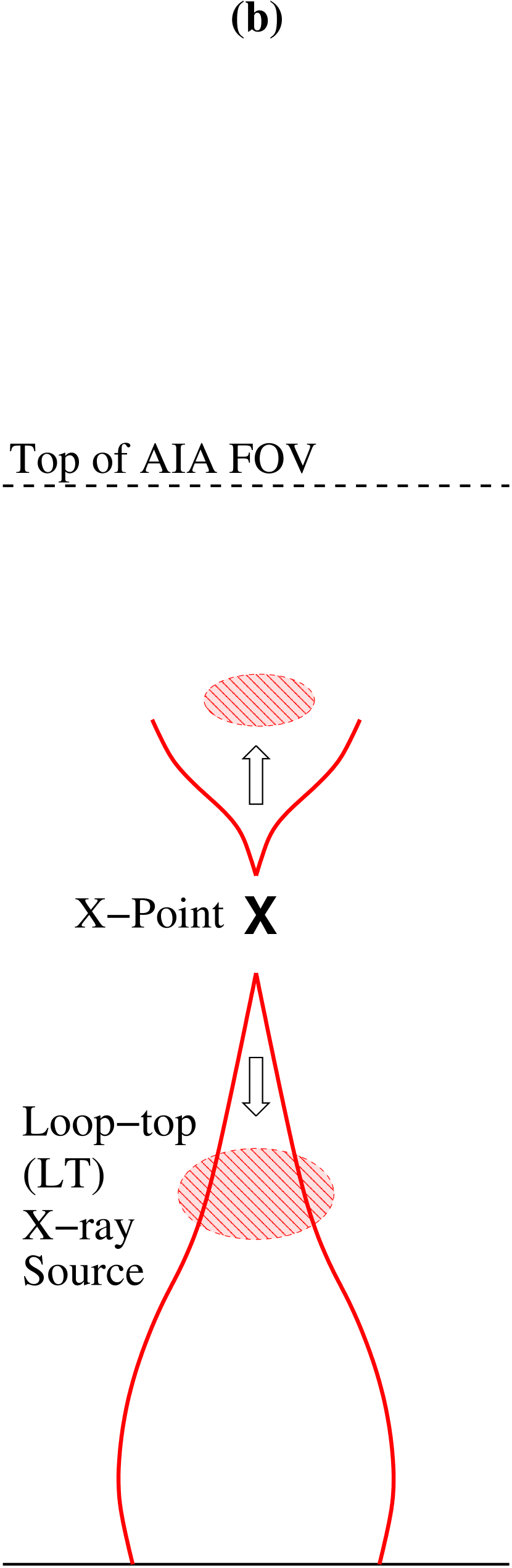
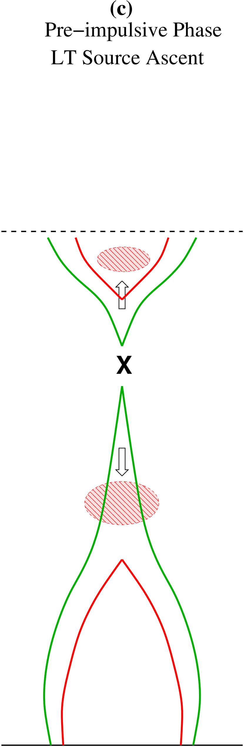
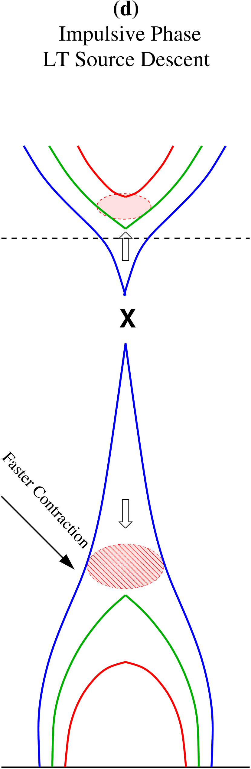
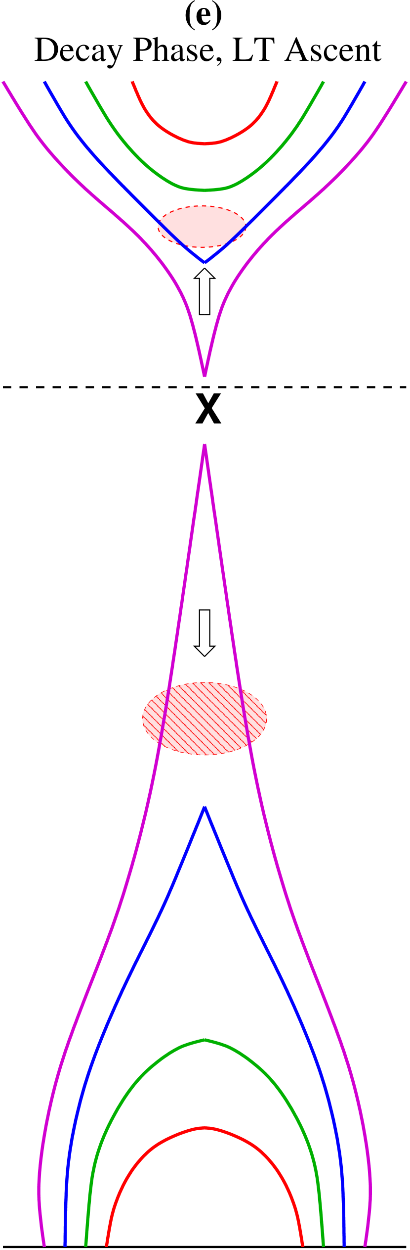
Figure 12.— (a) Schematic of the proposed flare model in which particle acceleration and plasma heating take place in the reconnection outflow regions away from the reconnection site. (b)–(e) Temporal development of reconnection and the up-down-up three-stage motion of the loop-top (LT) X-ray source. We show only the portions of reconnected magnetic field lines near the reconnection site, above and below which each pair of field lines are identified by the same color during their relaxations. Note that the higher contraction speeds (e.g., of the green loop) from (c) to (d) is associated with the loop-top source descent. The upper coronal source is not hatched during the impulsive and decay phases, indicating its non-detection due to weak emission. We assume that bi-directional reconnection outflows and relaxations of field lines persist throughout the event, but the upward component is beyond the AIA FOV during the late phase and thus not observed.

The earlier confined C4.5 flare leads to the formation of a flux rope and cusp-shaped loops underneath it. After six hours of slow evolution, the flux rope becomes unstable and rises (Patsourakos et al., 2013). A vertical current sheet forms between two Y-type null points at the lower tip of the flux rope and the upper tip of the underlying cusp. Magnetic reconnection ensues within the current sheet, leading to the eruptive M7.7 flare.

Magnetic reconnection produces bi-directional outflows in forms of the observed plasmoids and contracting loops. Plasmoids are flux tubes formed by the tearing mode (Furth et al., 1963) with a guiding field along the current sheet. They are magnetic islands in two dimension or when the current sheet is seen edge-on. These outflows are driven by the magnetic tension force of the highly bent, newly reconnected field lines, as in those pointed cusps. The outflows generally decelerate, as observed here, when they run into the ambient corona and when the contracting loops relax to less bent shapes with reduced magnetic tension. This implies that the low-altitude slow shrinkages could be the late stages of decelerated high-altitude fast contractions.

Several mechanisms can operate in the reconnection outflows and contribute to particle acceleration and plasma heating. Turbulence or plasma waves, for example, can be generated by the interaction of the high speed flows with the ambient corona. Upon cascading to smaller scales (comparable to the gyro-radii of background particles) at some distance from the reconnection site, turbulence can accelerate the particles and heat the plasma (Hamilton & Petrosian, 1992; Miller et al., 1996; Chandran, 2003; Petrosian & Liu, 2004; Petrosian et al., 2006; Jiang et al., 2009; Fleishman & Toptygin, 2013). Additional contribution to particle acceleration and/or heating can come from fast-mode shocks in the outflow regions (Forbes & Priest, 1983; Tsuneta & Naito, 1998; Guo & Giacalone, 2012; Nishizuka & Shibata, 2013), gas dynamic shocks within contracting flux tubes (Longcope et al., 2009), and the first-order Fermi and betatron mechanisms within the collapsing traps formed by contracting loops (Somov & Kosugi, 1997; Karlický & Kosugi, 2004; Karlický, 2006; Grady et al., 2012).

As the flux rope evolves into its fast rise and eruption stage, the current sheet could become sufficiently long causing significant tearing instability (e.g., Bárta et al., 2008), and/or become thinner than the ion skin depth leading to a transition from Sweet-Parker reconnection to collisionless Hall reconnection (Cassak et al., 2006). Both can result in enhanced rates of reconnection and energy release. The outflow velocity will also increase, producing stronger heating and particle acceleration by one or a combination of the above three mechanisms (turbulence, shock, and betatron) whose efficiency is expected to be positively correlated with the outflow velocity. For example, faster outflows can generate stronger turbulence that can lead to stronger particle acceleration (see Petrosian, 2012, for a comparison between acceleration by turbulence and shocks). This explains the observed temporal correlation of the increase in outflow velocity and the onset of the impulse phase and HXR burst.

The loop-top source seen in X-ray and EUV represents the collective emission of the ensemble of flare loops, each of which undergoes post-reconnection contraction or shrinkage. The loop-top emission centroid is the average position of this ensemble, which in the thermal regime is determined by the convolution of the spatial distributions of temperature and emission measure. Such distributions are influenced by several competing processes, including energization of new loops produced by the upward developing reconnection, and downward contractions and cooling of previously reconnected loops. We suggest that the interplay of these processes results in the up-down-up migration of the loop-top source. Around the early impulsive phase, the observed higher velocities of loop contractions tend to shift the overall loop-top source downward, as depicted in Figures 12(c) and (d). Within the contracting loops, conductive cooling can be considerably reduced by stronger turbulence produced by faster reconnection outflows (Chandran & Cowley, 1998; Jiang et al., 2006). Slower cooling helps the X-ray/EUV emission of these hot loops last longer during their contractions and further contribute to the loop-top descent. Before and after the early impulsive phase, the situation could be different. Loop contractions are slower and associated faster cooling can make these loops cool below the instrumental temperature passband more rapidly. The upward development of reconnection could thus dominate, leading to the upward loop-top migration. This interpretation is supported by the observed temporal coincidence of the highest velocities of individual loop shrinkages and of the loop-top descent at the impulsive phase onset. Like cooling, chromospheric evaporation can also play a role. After the initial chromospheric evaporation associated with energization of newly reconnected loops, if it continues operating during the subsequent loop contractions, the densities and thus emission measures of these loops would keep rising and contribute to the downward loop-top drift. Otherwise, if it rapidly subsides, it would assist the upward loop-top drift. Investigating such a complex interplay would require detailed numerical modeling, which is beyond our scope here.

6.3. Discussion

The fast downward contractions of EUV loops are best seen during the decay phase, likely because of their greater distances traveled making them easier to be detected. Likewise, different environments may explain the factor of two difference in the median deceleration between the early and later fast contractions (Figures 7(f) and (g)). The earlier, compact flare loops of stronger magnetic field can produce stronger resistance (e.g., by the Lorentz force from a reverse current; Bárta et al., 2008) to quickly brake the contracting loops impinging on them from above, while the later, large flare arcade of weaker field at greater heights and greater travel distances may allow more gradual deceleration.

The X-ray spectra are essentially thermal during the decay phase. This suggests that the late phase contractions are associated with plasma heating rather than particle acceleration. This is expected because the magnetic field strength decreases with height, and so does the available magnetic energy to be released by reconnection. Such prolonged heating may contribute to the well-known slower than expected cooling of flare plasma (see 1(d); McTiernan et al. 1993; Jiang et al. 2006).

The fast high-altitude contractions and slow low-altitude shrinkages appear as two statistically distinct populations. The median final velocity of the former is more than four times the median initial velocity of the latter ($-73$ vs. $-17\mathrm{\,km}\mathrm{\,s}^{-1}$; Figures 6 and 7). We have interpreted the latter as the late stages of the former that have decelerated, but we rarely see a continuous track decelerating from $>$$400\mathrm{\,km}\mathrm{\,s}^{-1}$ to a few $\mathrm{\,km}\mathrm{\,s}^{-1}$. Alternatively, this distinction may be due to inhomogeneity of reconnection (see, e.g., Asai et al., 2004) in the current sheet above the flare arcade that is primarily oriented along the line of sight. The persistent slow shrinkages could result from reconnection at a moderate rate throughout the current sheet, which produces flare loops forming the arcade and double ribbons at their footpoints. The episodic fast contractions could be signatures of plasmoids within the current sheet, associated with enhanced reconnection and energy release rates. These fast contracting loops are dispersed along the line of sight amidst slowly shrinking loops, producing the observed effects (e.g., 7(b)).

There are other physically different (though not necessarily unrelated) phenomena that share similar observational signatures and should not be confused with the contractions of newly reconnected loops studied here. For example, pre-existing coronal loops can contract at typical speeds $<$$100\mathrm{\,km}\mathrm{\,s}^{-1}$ during eruptions (Liu & Wang, 2010; Liu et al., 2012a; Sun et al., 2012), interpreted as implosion (Hudson, 2000; Janse & Low, 2007) due to the rapid release of magnetic energy and thus reduction of magnetic pressure within the eruption volume. When a CME eruption initiates at an elevated height, it can produces a downward push to displace ambient coronal loops (e.g., Liu et al., 2012c, see their Figure 12(h), at $-60\mathrm{\,km}\mathrm{\,s}^{-1}$). Even slower shrinkage at $-3\mathrm{\,km}\mathrm{\,s}^{-1}$ can occur in active region loops due to gradual cooling (Wang et al., 1997). Sometimes, conjugate X-ray footpoints approach each other while the loop-top source descends (Ji et al., 2006; Liu et al., 2009a; Yang et al., 2009), likely because of reconnection progressing toward less sheared loops at lower altitudes. We have not found these signatures in the flare under study here, except for a few overlying existing loops that contract at about $-150\mathrm{\,km}\mathrm{\,s}^{-1}$ during 05:40–05:50 UT near the end of the impulsive phase. In addition, some high-lying loops continue to expand and erupt at $\sim$$100\mathrm{\,km}\mathrm{\,s}^{-1}$ up to 08:00 UT, three hours after the original flux rope eruption. Examination of such features and quantitative comparison of these observations with particle acceleration models will be subjects of future investigations.

Appendix A
Observations of All AIA Channels

In the main text, we focused on the 131 Å channel. For a complete temperature coverage, we examine all AIA channels here. As shown in 13 (top), each channel has a generally broad response with one to a few peaks. In the order of approximately decreasing temperature response are 193, 131, 94, 304, 335, 211, and 171 Å channels.

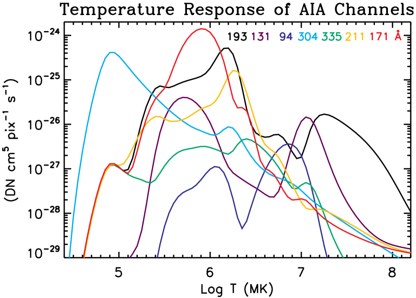
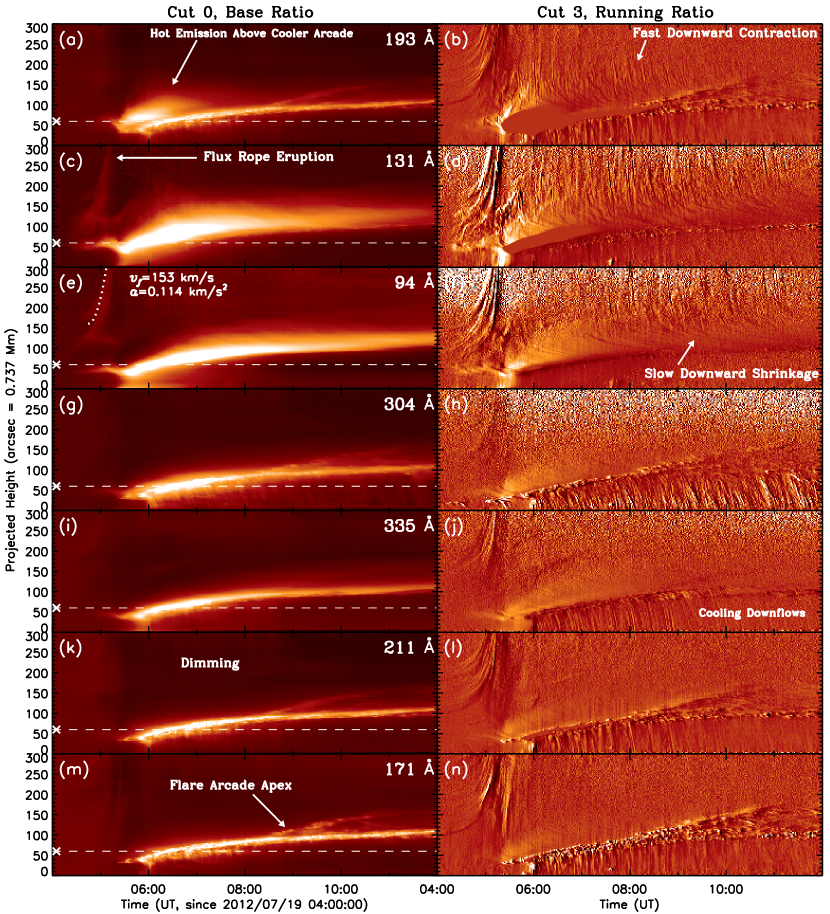
Figure 13.— Top: Temperature response of AIA EUV channels. Other panels: Space-time plots of all AIA EUV channels in base ratio from Cut 0 on the left and in running ratio from Cut 3 on the right. The panels are arranged approximately in the order from high to low temperature response. The cross and horizontal dash line on the left mark the slice for obtaining the temporal profiles shown in 1(b). The dotted line in (e) is a parabolic fit to the central portion of the erupting flux rope CME that has an average acceleration of $a=0.114\pm 0.002\mathrm{\,km}\mathrm{\,s}^{-2}$ and achieves a velocity of $v_{f}=153\pm 3\mathrm{\,km}\mathrm{\,s}^{-1}$ at the edge of AIA’s FOV.

13 shows space-time plots of all EUV channels. On the left are base ratio from every other frame of short exposure so that bright flare loops are not over-exposed, while on the right are running ratio from frames of regular exposure that is needed for detecting faint emission, including fast loop contractions, above the flare arcade. On the left, the 131 and 94 Å channels capture the hot, diffuse loop-top emission, while the flare arcade underneath it is best seen in cooler channels. Both regions appear in the 193 Å channel because of its dual response to hot Fe XXIV emission peaking at $18\mathrm{\,MK}$ and cool Fe XII emission at $1.6\mathrm{\,MK}$ (O’Dwyer et al., 2010). On the right-hand side, downward fast contractions and slow shrinkages can be identified in the three hottest channels. In cooler channels, cooling condensations rain down the arcade loops since 06:00 UT at up to $\sim$$170\mathrm{\,km}\mathrm{\,s}^{-1}$ or 90% of the free fall speed, faster than typical coronal rain (Antolin & Rouppe van der Voort, 2012).

In 13 (left), the erupting flux rope is best seen in the hot 131 and 94 Å channels as a bright, accelerating track, indicating its high temperature, as also shown in 11. Its evolution from gradual rise to impulsive eruption is accompanied by the rapid increase in X-ray flux and the loop-top’s ascent-to-descent transition. This is in line with observed synchronous eruption accelerations and flare onsets (Zhang et al., 2001, 2002; Temmer et al., 2008; Liu et al., 2011a).

Figures 1(b) and 4(a) show temporal emission profiles taken from the base-ratio space-time plots at $h_{\rm ref}=60\arcsec$ marked by a cross. Since 04:17 UT, the 131 and 94 Å emission increases considerably, while other emission remains essentially flat. This indicates gentle heating early in the flare, as seen in the temperature history at this position shown in 11(j). The dip in all channels at the onset of the impulsive phase (vertical dashed line) is due to the descent of the loop-top source. The large hump afterwards results from the growth of the flare arcade toward greater heights. This hump generally progresses toward cooler channels, indicating a cooling sequence, similar to those recently observed in flares, AR loops, and prominence condensations (Woods et al., 2011; Viall & Klimchuk, 2012; Liu et al., 2012b; Berger et al., 2012). The double humps at 193 Å are again due to its dual temperature response.

Like 193 Å, the 304 Å channel responds to both hot Ca XVIII emission at $7.1~{}\mathrm{\,MK}$ and cool He II emission at $0.05\mathrm{\,MK}$. The dual response of these two channels leads to their unusually large descent of about 40% of the loop-top centroids (see Table 2). This is because their maximum loop-top heights are dominated by hot emission, while the minimum heights are dominated by cool emission at even lower heights (4).

Appendix B
Disambiguation With STEREO Observations

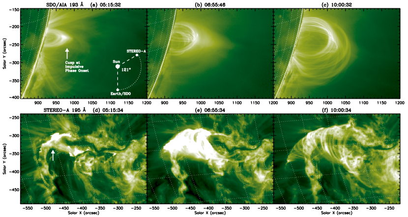
Figure 14.— Comparison of SDO/AIA 193 Å (top) and STEREO-A 195 Å (bottom) images of the flare. The STEREO images are scaled as if they are viewed from the same heliocentric distance as SDO. The heliographic grids are spaced at $5^{\circ}$. Note the compact brightening at the impulsive phase onset (pointed by the arrow), in contrast to the extended arcade system later.

The limb view of SDO/AIA leaves an alternative possibility of the loop-top descent as the progression of energization from high- to low-lying loops along the arcade in the east-west direction. This possibility is not supported by STEREO-A (STA) that was $121^{\circ}$ ahead of the Earth and observed the flare on the disk. When the X-ray loop-top descent occurs, the STA 195 Å image (14(d)) shows a compact cusp-shaped loop, while the arcade system develops later (panels (e) and (f)). One could further argue that a temperature effect, i.e., cooling or heating, can make a progression appear as a compact source rather than an arcade. If so, the loops being cooled or heated would have appeared at the same location and been captured by AIA in cooler or hotter EUV channels or by RHESSI in X-rays. Instead, all available EUV and X-ray data covering a wide temperature range of $10^{5}$–$10^{7}\mathrm{\,K}$ show a consistent loop-top descent, which must be a real mass motion.

References

- Antolin & Rouppe van der Voort (2012) Antolin, P. & Rouppe van der Voort, L. 2012, ApJ, 745, 152
- Asai et al. (2004) Asai, A., Yokoyama, T., Shimojo, M., & Shibata, K. 2004, ApJ, 605, L77
- Aschwanden et al. (2011) Aschwanden, M. J., Boerner, P., Schrijver, C. J., & Malanushenko, A. 2011, Sol. Phys., 384
- Bain et al. (2012) Bain, H. M., Krucker, S., Glesener, L., & Lin, R. P. 2012, ApJ, 750, 44
- Bárta et al. (2008) Bárta, M., Vršnak, B., & Karlický, M. 2008, A&A, 477, 649
- Battaglia et al. (2009) Battaglia, M., Fletcher, L., & Benz, A. O. 2009, A&A, 498, 891
- Battaglia & Kontar (2012) Battaglia, M. & Kontar, E. P. 2012, ApJ, 760, 142
- Berger et al. (2012) Berger, T. E., Liu, W., & Low, B. C. 2012, ApJ, 758, L37
- Carmichael (1964) Carmichael, H. 1964, in The Physics of Solar Flares, ed. W. N. Hess, 451
- Caspi & Lin (2010) Caspi, A. & Lin, R. P. 2010, ApJ, 725, L161
- Cassak & Drake (2013) Cassak, P. A. & Drake, J. F. 2013, submitted to ApJ
- Cassak et al. (2006) Cassak, P. A., Drake, J. F., & Shay, M. A. 2006, ApJ, 644, L145
- Chandran (2003) Chandran, B. D. G. 2003, ApJ, 599, 1426
- Chandran & Cowley (1998) Chandran, B. D. G. & Cowley, S. C. 1998, Physical Review Letters, 80, 3077
- Chen & Petrosian (2012) Chen, Q. & Petrosian, V. 2012, ApJ, 748, 33
- Fleishman & Toptygin (2013) Fleishman, G. D. & Toptygin, I. N. 2013, MNRAS, 447
- Fletcher et al. (2011) Fletcher, L., Dennis, B. R., Hudson, H. S., et al. 2011, Space Sci. Rev., 159, 19
- Forbes & Acton (1996) Forbes, T. G. & Acton, L. W. 1996, ApJ, 459, 330
- Forbes & Priest (1983) Forbes, T. G. & Priest, E. R. 1983, Sol. Phys., 84, 169
- Furth et al. (1963) Furth, H. P., Killeen, J., & Rosenbluth, M. N. 1963, Physics of Fluids, 6, 459
- Glesener et al. (2012) Glesener, L., Krucker, S., & Lin, R. P. 2012, ApJ, 754, 9
- Grady et al. (2012) Grady, K. J., Neukirch, T., & Giuliani, P. 2012, A&A, 546, A85
- Guo & Giacalone (2012) Guo, F. & Giacalone, J. 2012, ApJ, 753, 28
- Haerendel (2009) Haerendel, G. 2009, ApJ, 707, 903
- Hamilton & Petrosian (1992) Hamilton, R. J. & Petrosian, V. 1992, ApJ, 398, 350
- Hara et al. (2011) Hara, H., Watanabe, T., Harra, L. K., Culhane, J. L., & Young, P. R. 2011, ApJ, 741, 107
- Hirayama (1974) Hirayama, T. 1974, Sol. Phys., 34, 323
- Holman (2012) Holman, G. D. 2012, Physics Today, 65, 56
- Holman et al. (2011) Holman, G. D., Aschwanden, M. J., Aurass, H., Battaglia, M., Grigis, P. C., Kontar, E. P., Liu, W., Saint-Hilaire, P., & Zharkova, V. V. 2011, Space Sci. Rev., 159, 107
- Hudson (2000) Hudson, H. S. 2000, ApJ, 531, L75
- Innes et al. (1997) Innes, D. E., Inhester, B., Axford, W. I., & Wilhelm, K. 1997, Nature, 386, 811
- Innes et al. (2003) Innes, D. E., McKenzie, D. E., & Wang, T. 2003, Sol. Phys., 217, 247
- Janse & Low (2007) Janse, Å. M. & Low, B. C. 2007, A&A, 472, 957
- Ji et al. (2006) Ji, H., Huang, G., Wang, H., Zhou, T., Li, Y., Zhang, Y., & Song, M. 2006, ApJ, 636, L173
- Jiang et al. (2006) Jiang, Y. W., Liu, S., Liu, W., & Petrosian, V. 2006, ApJ, 638, 1140
- Jiang et al. (2009) Jiang, Y. W., Liu, S., & Petrosian, V. 2009, ApJ, 698, 163
- Karlický (2006) Karlický, M. 2006, Space Sci. Rev., 122, 161
- Karlický & Kosugi (2004) Karlický, M. & Kosugi, T. 2004, A&A, 419, 1159
- Karpen et al. (2012) Karpen, J. T., Antiochos, S. K., & DeVore, C. R. 2012, ApJ, 760, 81
- Khan et al. (2007) Khan, J. I., Bain, H. M., & Fletcher, L. 2007, A&A, 475, 333
- Ko et al. (2003) Ko, Y.-K., Raymond, J. C., Lin, J., Lawrence, G., Li, J., & Fludra, A. 2003, ApJ, 594, 1068
- Kopp & Pneuman (1976) Kopp, R. A. & Pneuman, G. W. 1976, Sol. Phys., 50, 85
- Krucker et al. (2010) Krucker, S., Hudson, H. S., Glesener, L., White, S. M., Masuda, S., Wuelser, J.-P., & Lin, R. P. 2010, ApJ, 714, 1108
- Lemen et al. (2012) Lemen, J. R., Title, A. M., Akin, D. J., et al. 2012, Sol. Phys., 275, 17
- Li & Gan (2005) Li, Y. P. & Gan, W. Q. 2005, ApJ, 629, L137
- Li & Gan (2006) —. 2006, ApJ, 644, L97
- Li & Gan (2007) —. 2007, Advances in Space Research, 39, 1389
- Lin (2004) Lin, J. 2004, Sol. Phys., 222, 115
- Lin et al. (2005) Lin, J., Ko, Y.-K., Sui, L., Raymond, J. C., Stenborg, G. A., Jiang, Y., Zhao, S., & Mancuso, S. 2005, ApJ, 622, 1251
- Lin et al. (2002) Lin, R. P., Dennis, B. R., Hurford, G. J., et al. 2002, Sol. Phys., 210, 3
- Liu (2013) Liu, R. 2013, submitted to ApJ
- Liu et al. (2010) Liu, R., Lee, J., Wang, T., Stenborg, G., Liu, C., & Wang, H. 2010, ApJ, 723, L28
- Liu et al. (2012a) Liu, R., Liu, C., Török, T., Wang, Y., & Wang, H. 2012a, ApJ, 757, 150
- Liu & Wang (2010) Liu, R. & Wang, H. 2010, ApJ, 714, L41
- Liu et al. (2012b) Liu, W., Berger, T. E., & Low, B. C. 2012b, ApJ, 745, L21
- Liu et al. (2011a) Liu, W., Berger, T. E., Title, A. M., Tarbell, T. D., & Low, B. C. 2011a, ApJ, 728, 103
- Liu et al. (2004) Liu, W., Jiang, Y. W., Liu, S., & Petrosian, V. 2004, ApJ, 611, L53
- Liu et al. (2012c) Liu, W., Ofman, L., Nitta, N. V., Aschwanden, M. J., Schrijver, C. J., Title, A. M., & Tarbell, T. D. 2012c, ApJ, 753, 52
- Liu et al. (2009a) Liu, W., Petrosian, V., Dennis, B. R., & Holman, G. D. 2009a, ApJ, 693, 847
- Liu et al. (2008) Liu, W., Petrosian, V., Dennis, B. R., & Jiang, Y. W. 2008, ApJ, 676, 704
- Liu et al. (2009b) Liu, W., Petrosian, V., & Mariska, J. T. 2009b, ApJ, 702, 1553
- Liu et al. (2011b) Liu, W., Title, A. M., Zhao, J., Ofman, L., Schrijver, C. J., Aschwanden, M. J., De Pontieu, B., & Tarbell, T. D. 2011b, ApJ, 736, L13
- Liu et al. (2009c) Liu, W., Wang, T.-J., Dennis, B. R., & Holman, G. D. 2009c, ApJ, 698, 632
- Longcope et al. (2009) Longcope, D. W., Guidoni, S. E., & Linton, M. G. 2009, ApJ, 690, L18
- Masuda et al. (1994) Masuda, S., Kosugi, T., Hara, H., Tsuneta, S., & Ogawara, Y. 1994, Nature, 371, 495
- McKenzie & Hudson (1999) McKenzie, D. E. & Hudson, H. S. 1999, ApJ, 519, L93
- McTiernan et al. (1993) McTiernan, J. M., Kane, S. R., Loran, J. M., Lemen, J. R., Acton, L. W., Hara, H., Tsuneta, S., & Kosugi, T. 1993, ApJ, 416, L91
- Miller et al. (1996) Miller, J. A., Larosa, T. N., & Moore, R. L. 1996, ApJ, 461, 445
- Milligan & Dennis (2009) Milligan, R. O. & Dennis, B. R. 2009, ApJ, 699, 968
- Milligan et al. (2010) Milligan, R. O., McAteer, R. T. J., Dennis, B. R., & Young, C. A. 2010, ApJ, 713, 1292
- Murphy et al. (2012) Murphy, N. A., Miralles, M. P., Pope, C. L., et al. 2012, ApJ, 751, 56
- Nakariakov & Melnikov (2009) Nakariakov, V. M. & Melnikov, V. F. 2009, Space Sci. Rev., 149, 119
- Neupert (1968) Neupert, W. M. 1968, ApJ, 153, L59
- Nishizuka & Shibata (2013) Nishizuka, N. & Shibata, K. 2013, ArXiv e-prints
- Nishizuka et al. (2010) Nishizuka, N., Takasaki, H., Asai, A., & Shibata, K. 2010, ApJ, 711, 1062
- Nitta et al. (2010) Nitta, N. V., Freeland, S. L., & Liu, W. 2010, ApJ, 725, L28
- O’Dwyer et al. (2010) O’Dwyer, B., Del Zanna, G., Mason, H. E., Weber, M. A., & Tripathi, D. 2010, A&A, 521, A21
- Ofman et al. (2011) Ofman, L., Liu, W., Title, A., & Aschwanden, M. 2011, ApJ, 740, L33
- Patsourakos et al. (2013) Patsourakos, S., Vourlidas, A., & Stenborg, G. 2013, ApJ, 764, 125
- Petrosian (2012) Petrosian, V. 2012, Space Sci. Rev., 173, 535
- Petrosian & Liu (2004) Petrosian, V. & Liu, S. 2004, ApJ, 610, 550
- Petrosian et al. (2006) Petrosian, V., Yan, H., & Lazarian, A. 2006, ApJ, 644, 603
- Pick et al. (2005) Pick, M., Démoulin, P., Krucker, S., Malandraki, O., & Maia, D. 2005, ApJ, 625, 1019
- Raymond et al. (2012) Raymond, J. C., Krucker, S., Lin, R. P., & Petrosian, V. 2012, Space Sci. Rev., 173, 197
- Reeves et al. (2008) Reeves, K. K., Seaton, D. B., & Forbes, T. G. 2008, ApJ, 675, 868
- Reznikova et al. (2010) Reznikova, V. E., Melnikov, V. F., Ji, H., & Shibasaki, K. 2010, ApJ, 724, 171
- Savage et al. (2012) Savage, S. L., Holman, G., Reeves, K. K., Seaton, D. B., McKenzie, D. E., & Su, Y. 2012, ApJ, 754, 13
- Savage & McKenzie (2011) Savage, S. L. & McKenzie, D. E. 2011, ApJ, 730, 98
- Sheeley et al. (2004) Sheeley, Jr., N. R., Warren, H. P., & Wang, Y.-M. 2004, ApJ, 616, 1224
- Shen et al. (2011) Shen, C., Lin, J., & Murphy, N. A. 2011, ApJ, 737, 14
- Shen et al. (2008) Shen, J., Zhou, T., Ji, H., Wang, N., Cao, W., & Wang, H. 2008, ApJ, 686, L37
- Shen & Liu (2012) Shen, Y. & Liu, Y. 2012, ApJ, 753, 53
- Somov & Kosugi (1997) Somov, B. V. & Kosugi, T. 1997, ApJ, 485, 859
- Sturrock (1966) Sturrock, P. A. 1966, Nature, 211, 695
- Su et al. (2012) Su, Y., Dennis, B. R., Holman, G. D., Wang, T., Chamberlin, P. C., Savage, S., & Veronig, A. 2012, ApJ, 746, L5
- Sui & Holman (2003) Sui, L. & Holman, G. D. 2003, ApJ, 596, L251
- Sui et al. (2004) Sui, L., Holman, G. D., & Dennis, B. R. 2004, ApJ, 612, 546
- Sun et al. (2012) Sun, X., Hoeksema, J. T., Liu, Y., Wiegelmann, T., Hayashi, K., Chen, Q., & Thalmann, J. 2012, ApJ, 748, 77
- Švestka et al. (1998) Švestka, Z., Fárník, F., Hudson, H. S., & Hick, P. 1998, Sol. Phys., 182, 179
- Švestka et al. (1987) Švestka, Z. F., Fontenla, J. M., Machado, M. E., Martin, S. F., & Neidig, D. F. 1987, Sol. Phys., 108, 237
- Takasao et al. (2012) Takasao, S., Asai, A., Isobe, H., & Shibata, K. 2012, ApJ, 745, L6
- Tandberg-Hanssen & Emslie (1988) Tandberg-Hanssen, E. & Emslie, A. G. 1988, The physics of solar flares (Cambridge and New York: Cambridge University Press, 286 p.)
- Temmer et al. (2008) Temmer, M., Veronig, A. M., Vršnak, B., Rybák, J., Gömöry, P., Stoiser, S., & Maričić, D. 2008, ApJ, 673, L95
- Tsuneta & Naito (1998) Tsuneta, S. & Naito, T. 1998, ApJ, 495, L67
- Veronig et al. (2006) Veronig, A. M., Karlický, M., Vršnak, B., Temmer, M., Magdalenić, J., Dennis, B. R., Otruba, W., & Pötzi, W. 2006, A&A, 446, 675
- Viall & Klimchuk (2012) Viall, N. M. & Klimchuk, J. A. 2012, ApJ, 753, 35
- Vršnak et al. (2006) Vršnak, B., Temmer, M., Veronig, A., Karlický, M., & Lin, J. 2006, Sol. Phys., 234, 273
- Wang et al. (1997) Wang, J., Shibata, K., Nitta, N., Slater, G. L., Savy, S. K., & Ogawara, Y. 1997, ApJ, 478, L41
- Wang et al. (2007) Wang, T. J., Sui, L., & Qiu, J. 2007, ApJ, 661, L207
- Wang et al. (1999) Wang, Y.-M., Sheeley, N. R., Howard, R. A., St. Cyr, O. C., & Simnett, G. M. 1999, Geophys. Res. Lett., 26, 1203
- Warren et al. (2011) Warren, H. P., O’Brien, C. M., & Sheeley, Jr., N. R. 2011, ApJ, 742, 92
- Watanabe et al. (2012) Watanabe, T., Hara, H., Sterling, A. C., & Harra, L. K. 2012, Sol. Phys., 185
- Woods et al. (2011) Woods, T. N., Hock, R., Eparvier, F., et al. 2011, ApJ, 739, 59
- Yang et al. (2009) Yang, Y.-H., Cheng, C. Z., Krucker, S., Lin, R. P., & Ip, W. H. 2009, ApJ, 693, 132
- Yokoyama et al. (2001) Yokoyama, T., Akita, K., Morimoto, T., Inoue, K., & Newmark, J. 2001, ApJ, 546, L69
- Zhang et al. (2001) Zhang, J., Dere, K. P., Howard, R. A., Kundu, M. R., & White, S. M. 2001, ApJ, 559, 452
- Zhang et al. (2002) Zhang, M., Golub, L., DeLuca, E., & Burkepile, J. 2002, ApJ, 574, L97