Delay-induced cluster patterns in coupled Cayley tree networks

Abstract

We study effects of delay in diffusively coupled logistic maps on the Cayley tree networks. We find that smaller coupling values exhibit sensitiveness to value of delay, and lead to different cluster patterns of self-organized and driven types. Whereas larger coupling strengths exhibit robustness against change in delay values, and lead to stable driven clusters comprising nodes from last generation of the Calaye tree. Furthermore, introduction of delay exhibits suppression as well as enhancement of synchronization depending upon coupling strength values. To the end we discuss the importance of results to understand conflicts and cooperations observed in family business.

1 Introduction

Many real-world networks display local co-ordination among nodes leading to cluster synchronization Nature2010 ; Science2010 ; SJ_prl2003 ; Kurths_prl2006 . Formation of clusters, which are based on the dynamical properties of the coupled system, typically depends on the underlying network structure. The interplay between the structure and the dynamics of complex networks has been a focus of intense research interest in last decades functional_net . Furthermore, delay naturally arises in extended systems due to the finite speed of information transmission book_delay . For example, in neural networks, propagation delays of electrical signals connecting different neurons and local neurovascular couplings lead to time delays book_neural1 ; book_neural3 . A delay may give rise to many new phenomena in dynamical systems such as oscillation death, enhancement or suppression of synchronization, chimera state, etc osc_death_delay ; delay_supress_syn ; delay_enhance_syn ; delay_coup_osc ; chimera . The existence of delay can completely change the behavior of a system as observed for undelayed case book_delay . What follows that time delay might be deliberately implemented in order to achieve desired functions such as secure communication secure_comm and to control neural disturbances, e.g., suppression of undesired synchrony of firing neurons in Parkinson’s disease or epilepsy neural_disease_delay1 ; neural_disease_delay2 ; neural_disease_delay3 .

Our recent work demonstrated that delay plays a crucial role in formation of synchronized clusters and mechanism behind the synchronization. We presented results for cluster formation in delayed coupled maps on 1-d lattice, small-world, scale-free, random and complete bipartite networks Singh2012 . In this paper we investigate delay-induced cluster patterns in diffusively coupled logistic maps on Cayley tree networks.

The Cayley tree is an infinite dimensional regular graph with an idealized hierarchical structure rev_network . Its rich hierarchal structure turns out to be an ideal model network to investigate driven patterns in details. Furthermore, regularity of Cayley trees makes analytical understanding or origin of driven patterns easier to understand using Lyapunov function analysis.

Cayley trees provide a simple model to do exact analysis for stability of synchronized states CML_tree , to study localization criteria in impurity atom solving_prob , to derive expression for magnetization and zero field susceptibility cayley_Ising , etc.. Biologically oriented work on Cayley tree networks include modeling of immune networks with antibody dynamics cayley_immune . In a recent paper, Cayley trees have been used to investigate Bose-Einstein condensation cayley_bose-condensation .

2 Model

We use well known delayed coupled maps model Singh2012 :

$$x_{i}(t+1)=(1-\varepsilon)f(x_{i}(t))+\frac{\varepsilon}{k_{i}}\sum_{j=1}^{N}A_{ij}g(x_{j}(t-\tau))$$ (1)

Here $k_{i}$ = $\sum_{j=1}^{N}A_{ij}$ is degree, and $x_{i}(t)$ is the dynamical variable of the $i-th$ node ($1\leq i\leq N$) at time $t$, $A$ is the adjacency matrix with elements $A_{ij}$ taking values $1$ and $0$ depending upon whether there is a connection between $i$ and $j$ or not. The delay $\tau$ is the time it takes for the information from a unit to reach its neighbors and be processed. The function $f(x)$ defines the local nonlinear map and the function $g(x)$ defines the nature of coupling between the nodes. We present the results for the local dynamics given by the logistic map $f(x)=\mu x(1-x)$ and for diffusive coupling $g(x)=f(x)$. We take $\mu=4$, for which logistic map exhibits chaotic behavior.

3 Phase synchronization and synchronized clusters

Synchronization of coupled dynamical systems is defined by the appearance of some relation between the functional of different dynamical variables. The exact synchronization corresponds to the situation where the dynamical variables for different nodes have identical values. The phase synchronization corresponds to the situation where the dynamical variables for different nodes have some definite relation between their phases phase_syn . We consider phase synchronization as defined in SJ_prl2003 ; phase_syn_prl1998 .

Phase synchronized clusters: Let $n_{i}$ and $n_{j}$ denote the number of times the variables $x_{i}(t)$ and $x_{j}(t)$, $t=1,2,\ldots T$ for the nodes $i$ and $j$, show local minima during the time interval $T$. Let $n_{ij}$ denote the number of times these local minima match with each other. Phase distance between two nodes $i$ and $j$ is given as $d_{ij}=1-2n_{ij}/(n_{i}+n_{j})$. Clearly, $d_{ij}=0$ when all minima of variables $x_{i}$ and $x_{j}$ match with each other $d_{ij}=1$ when none of the minima match. Nodes $i$ and $j$ are phase synchronized if $d_{ij}=0$. A cluster of nodes is phase synchronized if all pairs of nodes of the cluster are phase synchronized.

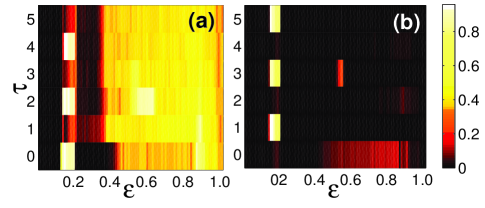
Figure 1: (Color online) Phase diagram demonstrating different values of (a) $f_{inter}$ and (b) $f_{intra}$ in two parameter space of $\varepsilon$ and $\tau$ ((a) and (b) ) with $N=127$, $<k>=2$. Local dynamics is governed by logistic map $f(x)=4x(1-x)$ and coupling function $g(x)=f(x)$. The figure is obtained by averaging over 20 random initial conditions. The color-scale encoding represents values of $f_{inter}$ and $f_{intra}$. The regions, which are black in both graphs (a) and (b), correspond to states of no cluster formation. The regions, where both subfigures have gray shades (yellow), correspond to states where clusters with both inter- and intra-couplings are formed. The regions in (a), which are lighter as compared to the corresponding $\varepsilon$ and $\tau$ values in (b), refer to dominant D phase synchronized clusters states, and the reverse refer to dominant SO phase synchronized clusters state. White (light yellow) regions in (a) and (b) refer to ideal D and ideal SO clusters state respectively. The regions, which are dark gray in (a) and black in (b) or vice-versa, correspond to states where very few nodes are forming the cluster.

4 Mechanisms of cluster formation

Depending upon the asymptotic dynamical behavior the nodes of the network can be divided into the following three types pre2005a .
(a) Cluster node synchronizes with other nodes and forms a synchronized cluster. Once this node enters a synchronized cluster it remains in that cluster afterwards.
(b) Isolated node does not synchronized with any other node and remains isolated all the time.
(c) Floating node keeps on switching intermittently between an independent evolution and a synchronized evolution attached to a cluster.

The study of relation between the synchronized clusters and the coupling between the nodes represented by the adjacency matrix exhibits following two different phenomena of cluster formation.
(1) Self-organized clusters: The nodes of a cluster can be synchronized because of intra-cluster couplings. We refer to this as the self-organized (SO) synchronization and the corresponding synchronized clusters as SO clusters. Ideal SO synchronization refers to a state when clusters do not have any connection outside the cluster, except one. Dominant SO synchronization corresponds to the state when most of the connections lie inside the cluster.
͑(2) Driven clusters: The nodes of a cluster can be synchronized because of inter-cluster couplings. We refer this as driven (D) synchronization and the corresponding cluster as D cluster. The ideal D synchronization refers to the state when clusters do not have any connections within them, and all connections are outside. Dominant D synchronization corresponds to the state when most of the connections lie outside the cluster and very few inside.

To get a clear picture of self-organized and driven behavior we consider two quantities $f_{intra}$ and $f_{inter}$ as measures for intra-cluster and inter-cluster couplings as follows:

$$f_{intra}=\frac{N_{intra}}{N_{c}},\,\,\,\,\,\,\,f_{inter}=\frac{N_{inter}}{N_{c}}$$ (2)

where $N_{intra}$ and $N_{inter}$ are the numbers of intra- and inter- cluster couplings, respectively. In $N_{inter}$, coupling between two isolated nodes are not included.

We define one more important state which forms basic backbone of the present investigation.
Cluster patterns: A cluster pattern refers to a particular phase synchronized state, which contains information of all the pairs of phase synchronized nodes distributed in various clusters. A cluster pattern can be static or dynamical. Static pattern has all nodes fixed, except few floating nodes, in a cluster with respect to change in time, delay value or initial condition. Dynamical pattern exhibits changes with time evolution, or with initial condition or with change in delay value. A change in the pattern refers to the state when members of a cluster get changed. Furthermore, patterns can be of D or SO type, which respectively refers to a particular D or SO phase synchronized state.

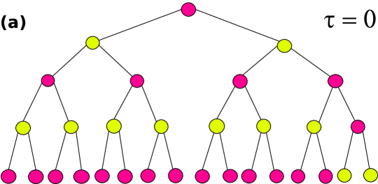
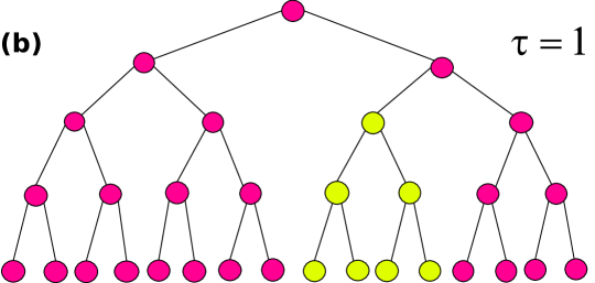
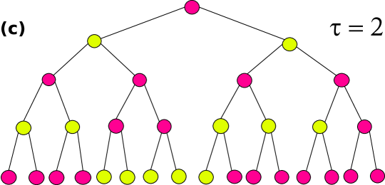
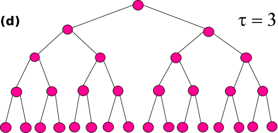
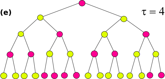
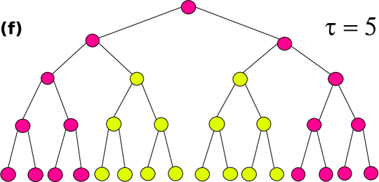
Figure 2: (Color online) Schematic network diagrams illustrating different cluster patterns observed for different delay values at lower coupling strength region. The examples are for $N=31,<k>=2$ and $\varepsilon=0.16$. The closed circles of same shade (color) imply that the corresponding nodes are phase synchronized (i.e. $C_{ij}=1$), and the open circles imply that the corresponding nodes are not phase synchronized.The D chaotic clusters for $\tau=0,2$ and $4$. The SO periodic clusters for $\tau=1$, $3$ and $5$.

5 Numerical Results

We evolve Equation (1) starting from random initial conditions, and study the dynamical behavior of nodes after an initial transient. We study phase synchronized clusters for $100$ time steps after the initial transient, and calculate values of $f_{inter}$ and $f_{intra}$ as described earlier.

Phase diagrams Figs.(1a) and (1b) are plotted for network size $N=127$ and average degree $<k>=2$. Undelayed Cayley tree exhibits dominant D clusters in the range $0.12\lesssim\varepsilon\lesssim 0.19$ with a periodic dynamical evolution. With a further increase in coupling strength, there is no phase synchronization till $\varepsilon=0.4$, after which dominant D clusters are obtained as elucidated by light gray (yellow) regions in Fig. (1a) and dark gray (red) regions in Fig. (1b). At very high coupling strengths, persistence of light gray (yellow) regions in (1a) and appearance of black regions in (1b) indicate ideal D clusters.

On introduction of a delay $\tau=1$ in the evolution equation Eq. 1, after very small coupling values for which there is no phase synchronization (black color for the subfigures  (1a) and (1b)), SO phase synchronized clusters are formed for $0.12{\lesssim}\varepsilon\lesssim 0.19$ as elucidated by white regions in (1b). As coupling strength increases, in the range $0.36\lesssim\varepsilon\lesssim 0.42$, where undelayed system exhibits no or very less cluster formation, delayed evolution manifests dominant D clusters as depicted by gray (yellow) regions in Fig. (1a). With a further increase in coupling strength, appearance of gray (yellow) regions in Fig. (1a) and black regions in Fig. (1b) indicate ideal D clusters.

For $\tau=2$, appearance of white (light yellow) window in Fig. (1a) and corresponding window in (1b) with dark gray (red) to black shades indicate formation of dominant and ideal D clusters respectively in lower coupling values. This description is same as observed for $\tau=0$. Larger coupling strengths lead to ideal D clusters as elucidated by black and light gray (yellow) regions in Figs. (1b) and (1a) respectively.

For a further increase in delay, at lower coupling strength odd delay values exhibit similar behavior as observed for $\tau=1$, while even delay values manifest similar behavior as observed for $\tau=0$ and $\tau=2$. At higher coupling values, coupled dynamics for all delays demonstrate either ideal or dominant D clusters.

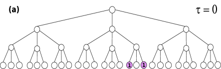
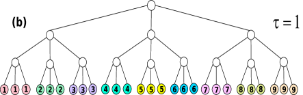
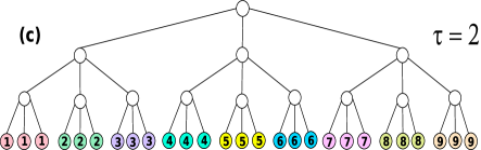
Figure 3: (Color online) Schematic diagrams illustrating delay-induced driven patterns for larger coupling values. The examples are for $N=40,<k>=3$ and $\varepsilon=0.37$. The closed circles of same number (same color) imply that the corresponding nodes are phase synchronized (i.e. $A_{ij}=1$), and the open circles imply that the corresponding nodes are not phase synchronized.The D chaotic clusters for $\tau=1,2$

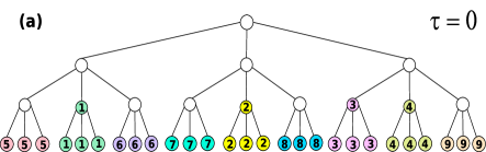
Figure 4: (Color online) Schematic diagrams illustrating effects on delay on phase synchronized patterns. The examples are for $N=30,<k>=3$ and $\varepsilon=0.7$. Closed circles having same number (same color) imply that corresponding nodes are phase synchronized in same cluster, and open circles imply that corresponding nodes are not phase synchronized.

5.1 Delay-induced change in mechanism of cluster formation:

Above discussions indicate that at the lower coupling values, change in delay values are related with the change in mechanism behind the cluster formation. Odd delay values lead to ideal or dominant SO clusters, whereas even delay values are associated with ideal or dominant D clusters. Figs. (2a), (2c) and (2e) illustrate that for $\tau=0$, $\tau=2$ and $\tau=4$, nodes in alternate generations are synchronized with each other, except few cases where nodes in two consecutive generations (parents and children) too exhibit synchronization. Figs. (2b), (2d) and (2f) demonstrate that for $\tau=1$, $\tau=3$ and $\tau=5$, either one single cluster is formed spanning all nodes, or several clusters are formed with clusters consisting of nodes in consecutive generations.

The cluster patterns observed here are dynamical with respect to intimal condition as well as with delay value, but for a particular value of delay the phenomenon behind the synchronization in cluster-pattern is static and same parity of delay leads to same phenomenon of cluster synchronization. The dynamical evolution in this range of coupling strength is periodic for all delay values.

5.2 Delay-induced driven patterns

As described in earlier sections, for coupling range $0.35\lesssim\varepsilon{\lesssim}0.42$, undelayed coupled maps do not exhibit cluster formation, whereas delayed evolution leads to dominant D clusters. In order to explain different these dynamical cluster patterns clearly we make schematic diagram of dynamical clusters in Fig. (3). For undelayed evolution there is no co-ordination between any pair of nodes, and hence there is no cluster pattern as depicted by all empty circles in Fig. (3a). Introduction of delay induces co-ordination between nodes in the same sub-family of the last generation, as depicted by different clusters in Fig.( 3b). Further change in delay value does not have any measure impact on synchronized clusters state. These cluster patterns are stable with respect to time evolution, initial condition as well as change in delay value.

For a further increase in $\varepsilon$, delay destroys the co-ordination between the nodes which are connected, giving rise to ideal D patterns with again only last generation nodes being synchronized in several clusters (Fig.( 4b)). These patterns are too stable with respect to change in initial condition or change in delay value. Furthermore, delayed as well undelayed dynamical evolution in this range are associated with the chaotic evolution.

6 Lyapunov function analysis

As demonstrated above, while undelayed evolution in middle coupling strength exhibits some synchrony between children in last generation and their parents, and hence giving rise to SO clusters, delayed evolution yields only D cluster indicating loss of synchrony between parent and children. Introduction of delay destroys the synchronization between parents and children while keeping the co-ordination between children unaffected. In order to understand this behavior let us write down Lyapunov function for a pair of synchronized nodes as,

$$V_{ij}(t+1)=[(1-\epsilon)(f(x_{i}(t))-f(x_{j}(t)))+$$

$$\frac{\varepsilon}{\sum_{k=1}^{N}A_{ij}}\sum_{k=1}^{N}A_{ik}{g}(x_{k}(t-\tau))-$$

$$\frac{\varepsilon}{\sum_{k=1}^{N}A_{ij}}\sum_{k=1}^{N}A_{ik}{g}(x_{k}(t-\tau))]^{2}$$

Lyapunov function takes following simple form for two nodes originated from the same parent node,

$$V_{ij}(t+1)=[(1-\epsilon)(f(x_{i}(t))-f(x_{j}(t)))]^{2}$$

Above equation does not have any delay term. All this leads to the conclusion that if a pair of nodes originated from same parent are synchronized, the introduction of delay would not affect the synchrony between them. Introduction of delay only affects the connected nodes such as parent and children, as it removes the common term in their evolution equations, and hence may be a reason behind the destruction of co-ordination between them Singh2012 .

7 Conclusion

We have studied delay-induced patterns in coupled maps on Cayley tree networks. We demonstrate that different delay values manifest different cluster patterns at lower coupling values, where change in delay not only leads to a completely new pattern but also associated with different mechanisms behind the cluster formation. In middle coupling range, delayed evolution always exhibits D clusters. Though we always find either ideal or dominant D clusters in this range, the role of delay on evolution and co-ordinations among nodes are very different for different coupling values. For some coupling values where undelayed evolution does not exhibit any synchronization, a introduction of delay enhances synchronization between children in last generation yielding D clusters, whereas for some coupling values delay destroys existing synchrony between parents and children while keeping children coordinated, again giving rise to D clusters. These delay induced D clusters are stable with respect to the change in delay value and consists only last generation nodes. Lyapunov function analysis provides some hints about formation of stable D clusters in this region.

The model which we have considered here demonstrates that lower coupling strength in general favors synchronization in various generations in the family, as indicated by larger cluster size and by large number of nodes (almost all) participating in clusters. These clusters are sensitive with respect to external conditions such a time delay. Where as higher coupling strength leads to very drastic behavior such as formation of stable D clusters comprising only last generations. The origin of these stable D clusters for last generation nodes can be very well understood for Calaye three, where coupling environment of the last generation nodes belonging to same sub-family remains same, and hence gives rise to a stable driven cluster Singh2012 , whereas nodes originated from the same parent in any previous generation can not have same coupling environment unless their all children are synchronized with each other.

Coupling strengths can be interpreted as closeness or bonding among family members, for example lower coupling strengths can correspond to a situation where members live in nuclear families and do not share much details apart that they belong to a same big family. Where as larger coupling strengths can be treated as a situation where all members of a family live together as a joint family joint_family_India . Our results may be used to understand conflicts in brothers running a successful family business family_business , which on very simple terms can be attributed to the conflicts between their children (as shown in Figs.(3) and (4)), where as lower coupling strength keeps a warmer relation leading to cooperation in family (as seen for Fig. (2)). Lower coupling strength here can be considered as separating the business of siblings and cousins, which have been proven to increase cooperation between them family_business_conflict .

To conclude, we demonstrate that delay in spatially extended systems may lead to a completely different relation between the functional clusters and topology than exhibited by undelayed evolution, and hence provide an additional step towards ongoing research attributed to understand relation between these two. Since delay has already been emphasized to be important for many real world networks book_delay , the results presented in the paper is important to understand various different behaviors exhibited by these systems. Furthermore, observation of different cluster patterns as a function of delay may shed some light in understanding conflicts or cooperation in family business family_business_conflict_book .

References

- (1) T. Danino, O. Mondragón-Palomino, L. Tsimirin and J. Hasty, Nature 462, 326 (2010).
- (2) T. Gregor, K. Fujimoto, N. Masaki and S. Sawai, Science 328, 1021 (2010).
- (3) S. Jalan and R. E. Amritkar, Phys. Rev. Lett. 90, 014101, (2003).
- (4) C. Zhou, L. Zamora, C. C. Hilgetag and J. Kurths, Phys. Rev. Lett. 97 238103 (2006).
- (5) V. Eguiluz et. al., Phys Rev E 83, 056113 (2011); C. Zhou et. al. Phys. Rev. Lett. 97, 238103 (2006); P. Oikonomou and P. Cluzel, Nature Physics 2, 532 (2006); A. Rad et. al., Phys. Rev. Lett. 108, 228701 (2012).
- (6) M. Lakshmanan and D. Senthilkumar Dynamics of Nonlinear Time-Delay Systems, (Springer Berlin, 2010).
- (7) H. Haken, Brain Dynamics: Synchronization and Activity Pattern in Pulse-Coupled Neural Nets with Delays and Noise (Springer Verlag GmbH, Berlin 2006).
- (8) W. Gerstner and W. Kistler, Spiking neuron models (Cambridge University Press, Cambridge, 2002).
- (9) D. Reddy et. al., Phys. Rev. Lett. 80, 5109 (1998); N. Punetha et al, Phys. Rev. E 85, 046204 (2012).
- (10) E. Schöll et. al., Phil Trans. R. Soc. A 367, 1079 (2009).
- (11) M. Dhamala . et. al., Phys. Rev. Lett. 92, 0741404 (2004); F. Atay et. al., Phys. Rev. Lett. 92, 144101 (2004); M. Shrii et. al., EPL 98, 10003 (2012).
- (12) M. K. Sen et. al., J. Stat. Mech. 10 1742 (2010).
- (13) G. Sethia et. al., Phys. Rev. Lett. 100, 144102 (2008); S. Jalan et. al., Chaos 16, 033124 (2007); J. Sheeba et. al., Phys. Rev. E 81, 046203 (2010).
- (14) B. Mensour and A. Longtin, Phys. Lett. A 244, 59 (1998); T. M. Hoang, IEEE 4, 3 (2010).
- (15) S. J. Schiff, K. Jerger, D. H. Duong, T. Chang, M. L. Spano and W. L. Ditto, Nature (London) 370, 615 (1994).
- (16) M. G. Rosenblum and A. Pikovsky, Phys. Rev. Lett. 92 114102 (2004).
- (17) O. V. Popovych, C. Hauptmann and P. A. Tass, Phys. Rev. Lett. 94, 164102 (2005).
- (18) A. Singh, S. Jalan and J. Kurths (Submitted).
- (19) R. Albert and A.-L. Barabasi, Rev. Mod. Phys. 74, 47 (2002).
- (20) P. M. Gade, H. A. Cerdeira and R. Ramaswamy, Phys. Rev. E 52, 3 (1995).
- (21) R. A. van Saten, J. Phys. C:Solid State Phys. 15, L513 (1982).
- (22) T. Hasegawa and K. Nemoto, Phys. Rev. E 75, 026105 (2007).
- (23) R. W. Anderson, A. U. Neumann and A. S. Perelson, Bulletin of Mathematical Biology, 55, 1091 (1993).
- (24) F. Fidaleo, arXiv:1203.5522v2 (2012).
- (25) M. G. Rosenblum, A. S. Pikovsky and J. Kurths, Phys. Rev. Lett. 76, 1804 (1996).
- (26) F. S. de San Roman, S. Boccaletti, D. Maza and H. Mancini, Phys. Rev. Lett. 81, 3639 (1998).
- (27) S. Jalan, R. E. Amritkar and C. K. Hu. Phys. Rev. E 72, 016211 (2005).
- (28) R. Owens, Ethnology 10, 223 (1971).
- (29) J. L. Ward and S. Waichler, Families in Business 20 (2005); D. Denison, C. Lief and J. L. Ward, SAGE 17, 61 (2004).
- (30) J. L. Ward, Family Business Review 13, 271 (2000).
- (31) P. Z. poutziouris, K. X. Smyrnios and S. B. Klein, Handbook of Research on family Business ( Edward Elgar Publishing, 2008 ).