Perturbative Bottom-up Approach for Neutrino Mass Matrix in Light of Large $\theta_{13}$ and Role of Lightest Neutrino Mass

Abstract

We discuss the role of lightest neutrino mass ($m_{0}$) in the neutrino mass matrix, defined in a flavor basis, through a bottom-up approach using the current neutrino oscillation data. We find that if $m_{0}<10^{-3}{\rm eV}$, then the deviation $\delta M_{\nu}$ in the neutrino mass matrix from a tree-level, say tribimaximal neutrino mass matrix, does not depend on $m_{0}$. As a result $\delta M_{\nu}$’s are exactly predicted in terms of the experimentally determined quantities such as solar and atmospheric mass squared differences and the mixing angles. On the other hand for $m_{0}\mbox{\raisebox{-2.58334pt}{~{}$\stackrel{{\scriptstyle>}}{{\sim}}$~{}}}10^{-3}{\rm eV}$, $\delta M_{\nu}$ strongly depends on $m_{0}$ and hence can not be determined within the knowledge of oscillation parameters alone. In this limit, we provide an exponential parameterization for $\delta M_{\nu}$ for all values of $m_{0}$ such that it can factorize the $m_{0}$ dependency of $\delta M_{\nu}$ from rest of the oscillation parameters. This helps us in finding $\delta M_{\nu}$ as a function of the solar and atmospheric mass squared differences and the mixing angles for all values of $m_{0}$. We use this information to build up a model of neutrino masses and mixings in a top-down scenario which can predict large $\theta_{13}$ perturbatively.

I Introduction

Compelling evidences of neutrino oscillations observed in solar, atmospheric and reactor experiments indicate that neutrinos are massive and hence they mix with each other pontecorvo . In the basis where the charged lepton masses are real and diagonal, the mixing matrix is given by pmns :

$$U_{{\rm PMNS}}=\left(\begin{array}[]{ccc}c_{12}\,c_{13}&s_{12}\,c_{13}&s_{13}\,e^{-i\delta_{\rm CP}}\\ -c_{23}\,s_{12}-s_{23}\,c_{12}\,s_{13}\,e^{i\delta_{\rm CP}}&c_{23}\,c_{12}-s_{23}\,s_{12}\,s_{13}\,e^{i\delta_{\rm CP}}&s_{23}\,c_{13}\\ s_{23}\,s_{12}-c_{23}\,c_{12}\,s_{13}\,e^{i\delta_{\rm CP}}&-s_{23}\,c_{12}-c_{23}\,s_{12}\,s_{13}\,e^{i\delta_{\rm CP}}&c_{23}\,c_{13}\end{array}\right)P,$$ (4)

where $c_{ij}=\cos\theta_{ij}$, $s_{ij}=\sin\theta_{ij}$ and $\delta_{\rm CP}$ is the Dirac CP violating phase on which the oscillation probability depends. The diagonal matrix $P={\rm diag}(e^{i\phi_{1}},\,e^{i\phi_{2}},\,1)$, consists of two Majorana phases $\phi_{1}$ and $\phi_{2}$ which are not relevant in neutrino oscillation experiments Bilenky ; Langacker . However, they affect lepton number violating amplitudes such as neutrinoless double beta decay. Thus in a flavor basis, where charged leptons are real and diagonal, the neutrino mass matrix is given by:

$$M_{\nu}=U^{\ast}_{{\rm PMNS}}\,{\rm diag}(m_{1},\,m_{2},\,m_{3})\,U^{\dagger}_{{\rm PMNS}},$$ (5)

where $m_{1},\,m_{2},\,m_{3}$ are the mass eigenvalues.

In the last decade, data from solar and reactor neutrino experiments have provided information on the sign and magnitude of $\Delta m_{\odot}^{2}$ and a precise value of $\theta_{12}$ sno ; kamland . The atmospheric parameters $|\Delta m_{\rm atm}^{2}|$ and $\theta_{23}$ have been measured and their precision will be increased by T2K t2k and NO$\nu$A nova . The sign of solar mass splitting $\Delta m_{\odot}^{2}$ is precisely known, while the sign of atmospheric mass splitting $\Delta m_{\rm atm}^{2}$ is still unknown. This opens up a possibility of whether neutrino masses follow normal ordering, i.e., $m_{1}<m_{2}<m_{3}$ or inverted ordering, i.e., $m_{3}<m_{1}<m_{2}$. In other words, the lightest mass, either $m_{1}$ (normal ordering) or $m_{3}$ (inverted ordering) is yet to be determined. Recent measurement from T2K t2k2 , MINOS minos , Double Chooz DC , Daya Bay daya , and RENO reno confirms a non-zero value of $\theta_{13}$ at $5\sigma$ confidence level. This opens up a range of possibilities to measure the sign of the atmospheric mass splitting and the unknown CP phase $\delta_{CP}$.

The absolute mass scale of neutrino is hitherto not known and can only be measured in a tritium beta decay experiment. The KATRIN experiment, which will investigate the kinematics of tritium beta decay, aims to measure the neutrino mass with a sensitivity of $0.2\,{\rm eV}$ katrin . At present the best upper limit at $95\%$ confidence level on the sum of the neutrino masses comes from the cosmic microwave background data and is given by wmap9 :

$$\sum_{i}m_{i}<0.44eV\,.$$ (6)

Once the absolute mass scale of the lightest neutrino, either $m_{1}$ in normal ordering or $m_{3}$ in inverted ordering, is determined one can reconstruct the neutrino mass matrix in the flavor basis using the experimental values of the elements of $U_{{\rm PMNS}}$ matrix. This may unravel exact flavor structure in the neutrino mass matrix.

In light of recent non-zero $\theta_{13}$, a large number of flavor models have been proposed by using the top-down approach, where one assumes a specific symmetry symmetry_1 ; symmetry_2 ; symmetry_3 ; symmetry_4 ; symmetry_5 ; reviews to explain the observed masses and mixings of the light neutrinos. However, it is worth exploring the symmetries of neutrino mass matrix through a data driven approach data_drive_approach . But as we discussed above the mass of lightest neutrino is yet to be known and therefore, the low energy neutrino data may not unravel the full flavour structure.

In this paper we develop a perturbative bottom-up approach to unravel the flavor structure of neutrino mass matrix and discuss the role of lightest neutrino mass. We set the full neutrino mass matrix: $M_{\nu}=(M_{\nu})_{0}+\delta M_{\nu}$, where $\delta M_{\nu}$ is the perturbation around the tree-level mass matrix $(M_{\nu})_{0}$, which is determined using some of the well known mixing scenarios such as tribimaximal (TBM) mixing tbm , bimaximal (BM) mixing bm and/or democratic (DC) mixing dcm . Among all these, the TBM is closer to the experimentally observed mixing pattern and hence mostly studied. All these mixing scenarios, however, predict $\theta_{13}$ to be zero and hence ruled out by the recent measurement on the reactor neutrino angle. However, a perturbative approach to realize a large value of $\theta_{13}$ is still a viable option. So, we assume that the non-zero value of $\theta_{13}$ is generated perturbatively. Using the $3\sigma$ range of values of the elements of $U_{{\rm PMNS}}$ matrix we determine $\delta M_{\nu}$ as a function of the lightest neutrino mass, say $m_{0}$, where $m_{0}=m_{1}$ in the normal ordering and $m_{0}=m_{3}$ in the inverted ordering. In this way we find that for $m_{0}<10^{-3}$ eV, all the $\delta M_{\nu}$ are independent of $m_{0}$ and hence the lightest neutrino mass does not play any role in the perturbative determination of neutrino mass matrix. Such models, for example, can be generated in two right-handed neutrino extensions of the standard model (SM). However, for $m_{0}\mbox{\raisebox{-2.58334pt}{~{}$\stackrel{{\scriptstyle>}}{{\sim}}$~{}}}10^{-3}$ eV the lightest neutrino mass plays an important role in the perturbative determination of neutrino mass matrix. We factorize the $m_{0}$ dependency of $\delta M_{\nu}$ using an exponential parameterization: $\delta M_{\nu}(m_{0})\propto\delta M_{\nu}|_{m_{0}=0}{\rm Exp}[-m_{0}/0.1\,{\rm eV}]$. This helps us in finding the required perturbations of $\delta M_{\nu}$ as a function of experimentally determined quantities such as solar and atmospheric mass squared differences and the mixing angles. To this end we apply the result of bottom-up approach to develop a model which predict large $\theta_{13}$ perturbatively.

The paper is organized as follows. In section II.1, we start with a brief description of the bottom-up approach that is developed in this paper to find the desired perturbation of the mass matrix in the flavor basis. Then, in section II.2, we use the knowledge of our current experimental results to find the deviation in the tree-level mass matrix of the neutrinos, obtained by using TBM mixing ansatz. In section III, we use the result of bottom-up approach to develop a model in which the perturbation to the TBM mixing is obtained. We then fit the model parameters using the data from the bottom-up approach of section II.2 and conclude in section IV.

II Phenomenology

II.1 Bottom up approach

The recent global fit to the neutrino oscillation data has ruled out the possibility of a zero reactor angle at $10.2\sigma$ confidence level Tortola ; Schwetz . Evidence of non zero $\theta_{13}$ at $3\sigma$ level was first established by data from T2K t2k , MINOS minos and Double Chooz DC . More recently, Daya Bay daya and RENO reno experiments confirm large $\theta_{13}$ at more than $5\sigma$ confidence level (CL) from the reactor $\bar{\nu}_{e}\to\bar{\nu}_{e}$ oscillations. The current best fit values and the $3\sigma$ allowed values of all the mixing parameters are summarized in Table. 1.

Oscillation parameters	Best fit value	$3\sigma$ range
$\Delta m_{\odot}^{2}\left[10^{-5}\,{\rm eV^{2}}\right]$	$7.62$	$[7.12-8.20]$
$|\Delta m_{\rm atm}^{2}|\left[10^{-3}\,{\rm eV^{2}}\right]$	$2.55~{}(2.43)$	$[2.31-2.74]~{}([2.21-2.64])$
$\sin^{2}\,\theta_{12}$	$0.320$	$[0.27-0.37]$
$\sin^{2}\,\theta_{23}$	$0.613~{}(0.600)$	$[0.36-0.68]~{}([0.37-0.67])$
$\sin^{2}\,\theta_{13}$	$0.0246~{}(0.0250)$	$[0.017-0.033]$

Table 1: Current status of oscillation parameters taken from Ref. Tortola .

The values written within brackets are for inverted ordering of the neutrino mass spectrum. At this juncture we note that the only unknown quantity in the neutrino mass matrix is the lightest neutrino mass apart from the CP violating phases (one Dirac and two Majorana phases).

The neutrino mixing matrix derived from the current best fit parameters is

$$U^{c}_{{\rm EXPT}}=\left(\begin{array}[]{ccc}0.81442&0.55868&0.15684\\ -0.45317&0.44353&0.77325\\ 0.36244&-0.70083&0.61439\end{array}\right),$$ (10)

and the corresponding $3\sigma$ allowed values of the mixing matrix is

$$U_{{\rm EXPT}}=\left(\begin{array}[]{ccc}0.78-0.85&0.51-0.60&0.13-0.18\\ -(0.39-0.57)&0.36-0.64&0.59-0.82\\ 0.19-0.44&-(0.54-0.76)&0.56-0.79\end{array}\right)\,,$$ (14)

where we have assumed $\delta_{CP}$ to be zero for simplicity. The corresponding neutrino mass matrix in the flavor basis can be written as

$$(M_{\nu})_{{\rm EXPT}}=U_{{\rm EXPT}}\,{\rm diag}(m_{1},\,m_{2},\,m_{3})\,U^{T}_{{\rm EXPT}}$$ (15)

where $(M_{\nu})_{{\rm EXPT}}$ is a real symmetric matrix. Therefore, it is described by three masses: $m_{1},\,m_{2},\,m_{3}$ and three mixing angles: $\theta_{12},\,\theta_{23},\,\theta_{13}$. The mass eigenvalues $m_{1},\,m_{2},\,m_{3}$ in the basis where the charged leptons are real and diagonal can be expressed as: $m_{2}=\sqrt{\Delta m_{\odot}^{2}+m_{1}^{2}}$ and $m_{3}=\sqrt{\Delta m_{\rm atm}^{2}+m_{1}^{2}}$ for normal hierarchy and $m_{1}=\sqrt{m_{3}^{2}+\Delta m_{\rm atm}^{2}}$ and $m_{2}=\sqrt{m_{3}^{2}+\Delta m_{\rm atm}^{2}+\Delta m_{\odot}^{2}}$ for inverted hierarchy.

We define the perturbed neutrino mass matrix $\delta M_{\nu}$ as

$$\delta M_{\nu} = (M_{\nu})_{{\rm EXPT}}-(M_{\nu})_{0}\,,$$ (16)

where $(M_{\nu})_{{\rm EXPT}}$ is the neutrino mass matrix given by Eq. 15 and $(M_{\nu})_{0}$ is the neutrino mass matrix corresponding to a mixing matrix $U_{0}$, that is obtained in a specific model such as TBM mixing, BM mixing and/or DC mixing etc. This $\delta M_{\nu}$ is a symmetric matrix whose elements denote the amount of perturbation that is needed to add to the $(M_{\nu})_{0}$ so that it is consistent within the $3\sigma$ of the experimental results. In order to gauge the size of the $\delta M_{\nu}$ matrix, we do a random scan of all the parameters: $\theta_{13}$, $\theta_{23}$, $\theta_{12}$, $\Delta m_{\odot}^{2}$ and $|\Delta m_{\rm atm}^{2}|$ within their $3\sigma$ allowed range of values. Note that $(M_{\nu})_{0}$ depends only on the value of the lightest neutrino mass $m_{0}$ as the mixing angles are expected to be fixed via certain symmetries as done in TBM, BM and/or DC mixing scenarios. Hence, to see the effect of $m_{0}$ on the elements of $\delta M_{\nu}$ we vary $m_{0}$ in the range $[10^{-9},10]\,{\rm eV}$. We then define the predicted neutrino mass matrix $(M_{\nu})_{M}$ of any model as:

$$(M_{\nu})_{M} = (M_{\nu})_{0}+\delta M_{\nu}\,.$$ (17)

Note that the matrix elements of $(M_{\nu})_{M}$ and $\delta M_{\nu}$ are function of the oscillation parameters $\theta_{12}$, $\theta_{23}$, and $\theta_{13}$ as well as of the lightest neutrino mass $m_{0}$. We then perform a naive statistical analysis and compare the elements of the $(M_{\nu})_{M}$ to the experimental data of Eq. 15 by a $\chi^{2}$ function which is defined by:

$$\chi^{2} = \Big{[}(M_{\nu}^{c})_{{\rm EXPT}}-(M_{\nu})_{M}\Big{]}^{2}/m_{0}\sigma^{2}=\Big{[}\delta M_{\nu}^{c}-\delta M_{\nu}\Big{]}^{2}/m_{0}\sigma^{2}\,,$$ (18)

where $\sigma=\sqrt{(M_{\nu}^{c})_{{\rm EXPT}}}$ and $\delta M_{\nu}^{c}=(M_{\nu}^{c})_{{\rm EXPT}}-(M_{\nu})_{0}$. Note that $(M_{\nu}^{c})_{{\rm EXPT}}$ is the experimental mass matrix corresponding to the best fit values of the oscillation parameters and is diagonalized by the mixing matrix of Eq. 10. It is worth noting that as $\delta M_{\nu}\to\delta M_{\nu}^{c}$, we get the minimum $\chi^{2}$ and hence $\delta M_{\nu}^{c}$ is the required amount of perturbation that should be added to $(M_{\nu})_{0}$. We will discuss the properties of the $\delta M_{\nu}$ matrix using the TBM mixing ansatz. Although we focus mainly on the TBM mixing, some of the features presented here are applicable to other tree-level mass matrix.

II.2 Perturbation in Tribimaximal mixing Scenario

We now proceed to discuss the tribimaximal (TBM) mixing scenario. For the TBM mixing , we have $s_{12}=1/\sqrt{3}$, $s_{23}=1/\sqrt{2}$, and $s_{13}=0$. We know that apart from the recently measured value of $\theta_{13}$, the solar and atmospheric mixing angles are in a very good agreement with the TBM ansatz. Modifications to this TBM scenario have been studied by many authors tbmprtb .

We begin by writing the TBM mixing matrix in the standard parameterization of Eq. 4, that is

$$U_{{\rm TBM}} = \left(\begin{array}[]{ccc}\sqrt{2/3}&\sqrt{1/3}&0\\ -\sqrt{1/6}&\sqrt{1/3}&\sqrt{1/2}\\ \sqrt{1/6}&-\sqrt{1/3}&\sqrt{1/2}\end{array}\right)=\left(\begin{array}[]{ccc}0.81650&0.57735&0\\ -0.40825&0.57735&0.70711\\ 0.40825&-0.57735&0.70711\end{array}\right).$$ (25)

The corresponding neutrino mass matrix in the flavor basis and the perturbed matrix $\delta M_{\nu}$ are

$$(M_{\nu})_{{\rm TBM}} = U_{{\rm TBM}}\,{\rm diag}(m_{1},\,m_{2},\,m_{3})\,U^{T}_{{\rm TBM}}\,,\qquad\qquad\delta M_{\nu}=(M_{\nu})_{{\rm EXPT}}-(M_{\nu})_{{\rm TBM}}.$$ (26)

We wish to determine the elements of this $\delta M_{\nu}$ matrix in a bottom-up approach. We follow the procedure given in section II.1 and perform a random scan over all the oscillation parameters within their $3\sigma$ range of values. In Fig. 1, we show $\delta M_{\nu}(i,j)$ versus $\chi^{2}$ for $m_{0}=10^{-9}\,{\rm eV}$. The minimum of each curve corresponds to the value of $\delta M_{\nu}^{c}(i,j)$. A similar plot is shown in Fig. 2 for inverted hierarchy as well.

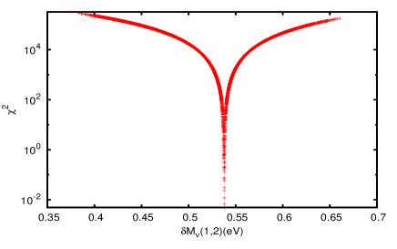
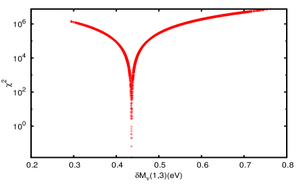
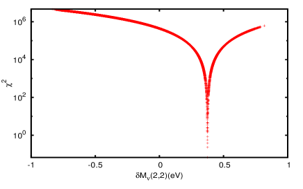
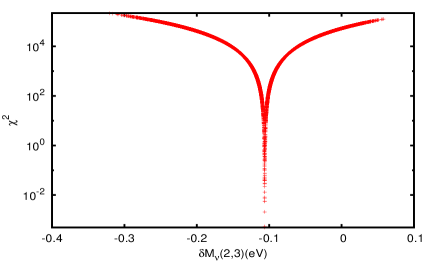
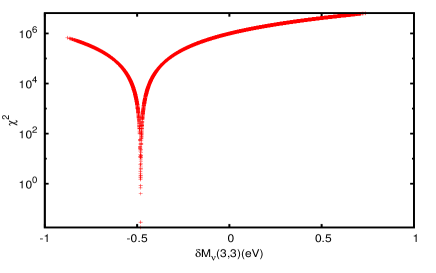
Figure 1: $\chi^{2}$ of $(\delta M_{\nu}(i,j)\times 10^{2})$ for normal ordering of neutrino masses with TBM mixing in tree-level.

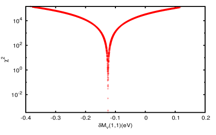
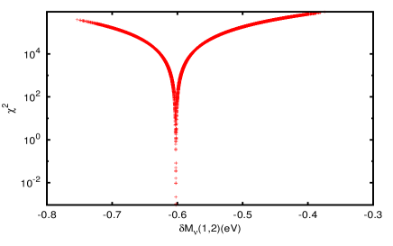
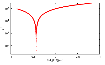
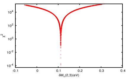
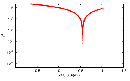
Figure 2: $\chi^{2}$ of $(\delta M_{\nu}(i,j)\times 10^{2})$ for inverted ordering of neutrino masses with TBM mixing in tree-level.

We know that the neutrino mass matrix in the flavor basis does depend on the value of the lightest mass eigenvalue $m_{0}$. In order to see the effect of $m_{0}$ on the value of $\delta M_{\nu}^{c}(i,j)$ qualitatively, we vary $m_{0}$ in the range $(10^{-10}$, $10)\,{\rm eV}$ while keeping other parameters such as $\theta_{12}$, $\theta_{13}$, $\theta_{23}$, $|\Delta m_{\rm atm}^{2}|$, and $\Delta m_{\odot}^{2}$ fixed at their best fit values. In Fig. 3, we plot $\delta M_{\nu}^{c}(i,j)$ versus $m_{0}$ and it is clear that for $m_{0}<10^{-3}\,{\rm eV}$, the value of $\delta M_{\nu}^{c}(i,j)$ remains constant. In other words, $\delta M_{\nu}(i,j)$ are independent of the value of $m_{0}$. However, for $m_{0}\mbox{\raisebox{-2.58334pt}{~{}$\stackrel{{\scriptstyle>}}{{\sim}}$~{}}}10^{-3}\,{\rm eV}$, the value of $\delta M_{\nu}(i,j)$ keeps changing. In the limit, $m_{0}>>\sqrt{|\Delta m_{\rm atm}^{2}|}=4.9\times 10^{-2}\,{\rm eV}$, we have $m_{3}=m_{2}=m_{1}=m_{0}$ and hence $\delta M_{\nu}(i,j)$ become zero. This particular feature is common to both normal and inverted hierarchies as can be seen from Fig. 3.

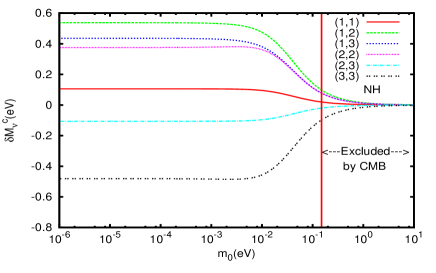
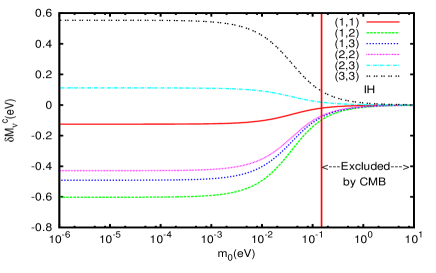
Figure 3: Variation of $(\delta M_{\nu}^{c}\times 10^{2})$ with respect to the lightest neutrino mass for NH (left) and IH (right) of neutrino masses with TBM mixing. An upper cut-off at $m_{0}\approx 0.15{\rm eV}$ wmap9 is put to ensure that $\delta M_{\nu}(i,j)\neq 0$ for all $m_{0}<0.15{\rm eV}$.

To appreciate the plots in Fig. 3, we write down $\delta M_{\nu}(i,j)$ as a function of neutrino masses and mixing angles:

$$\delta M_{\nu}(1,1) = ({(c_{12}c_{13})}^{2}-2/3)m_{1}+({(s_{12}c_{13})}^{2}-1/3)m_{2}+s^{2}_{13}m_{3}$$

$$\delta M_{\nu}(1,2) = (c_{12}c_{13}(-s_{12}c_{23}-c_{12}s_{23}s_{13})+1/3)m_{1}$$

$$+ (s_{12}c_{13}(c_{12}c_{23}-s_{12}s_{23}s_{13})-1/3)m_{2}+s_{13}c_{13}s_{23}m_{3}$$

$$\delta M_{\nu}(1,3) = (c_{12}c_{13}(s_{12}s_{23}-c_{12}c_{23}s_{13})-1/3)m_{1}$$

$$+ (s_{12}c_{13}(-c_{12}s_{23}-s_{12}c_{23}s_{13})+1/3)m_{2}+s_{13}c_{13}c_{23}m_{3}$$

$$\delta M_{\nu}(2,2) = ({(-s_{12}c_{23}-c_{12}s_{23}s_{13})}^{2}-1/6)m_{1}$$

$$+ ({(c_{12}c_{23}-s_{12}s_{23}s_{13})}^{2}-1/3)m_{2}+({(c_{13}s_{23})}^{2}-1/2)m_{3}$$

$$\delta M_{\nu}(2,3) = ((-s_{12}c_{23}-c_{12}s_{23}s_{13})(s_{12}s_{23}-c_{12}c_{23}s_{13})+1/6)m_{1}$$

$$+ ((c_{12}c_{23}-s_{12}s_{23}s_{13})(-c_{12}s_{23}-s_{12}c_{23}s_{13})+1/3)m_{2}+(s_{23}c_{13}c_{23}c_{13}-1/2)m_{3}$$

$$\delta M_{\nu}(3,3) = ({(s_{12}s_{23}-c_{12}c_{23}s_{13})}^{2}-1/6)m_{1}$$ (27)

$$+ ({(-c_{12}s_{23}-s_{12}c_{23}s_{13})}^{2}-1/3)m_{2}+({(c_{13}c_{23})}^{2}-1/2)m_{3}\,.$$

Note that the higher eigenvalues $m_{2}$ and $m_{3}(m_{1})$ can be re-expressed as a function of lightest neutrino mass $m_{0}\equiv m_{1}(m_{3})$. Therefore, it is obvious that all the elements: $\delta M_{\nu}(i,j)$ are function of the only unknown quantity $m_{0}$. From Fig. 3 we see that $\delta M_{\nu}(1,1)$, $\delta M_{\nu}(1,2)$, $\delta M_{\nu}(1,3)$, $\delta M_{\nu}(2,2)$ start with a positive value, while $\delta M_{\nu}(2,3)$ and $\delta M_{\nu}(3,3)$ start with a negative value. An exactly opposite spectrum is observed in case of inverted hierarchy as expected. In either case we observe that for $m_{0}<<10^{-3}{\rm eV}$, $\delta M_{\nu}(i,j)$ are independent of $m_{0}$. Therefore, in this limit it is reasonable to set $m_{0}\approx 0$.

In the opposite limit when $m_{0}>>\sqrt{|\Delta m_{\rm atm}^{2}|}=4.9\times 10^{-2}\,{\rm eV}$, we have $m_{3}=m_{2}=m_{1}=m_{0}$. In this limit we get $M_{\nu}(i,j)=m_{0}\,(I)$, where $I$ is the identity matrix. Hence all the $\delta M_{\nu}(i,j)$ are zero as expected . This feature can be easily read from Fig. 3. However, the observation tells us that this should not be the case and we need small mass splittings between the mass eigenvalues in order to satisfy the solar and atmospheric mass differences. Therefore, we put an upper cut-off at $m_{0}\approx 0.15{\rm eV}$ wmap9 , as required by CMB data, to ensure that $\delta M_{\nu}(i,j)\neq 0$ for all $m_{0}<0.15{\rm eV}$. In this region $m_{1}\neq m_{2}\neq m_{3}$.

For $10^{-3}\,{\rm eV}<m_{0}<0.15{\rm eV}$, which is comparable to solar and atmospheric values, we observe appreciable effect of $m_{0}$ on various $\delta M_{\nu}(i,j)$ as shown in Fig. 3. We have factored out this dependency of all $\delta M_{\nu}(i,j)$ on $m_{0}$ using an exponential parameterization:

$$\left|\delta M_{\nu}(m_{0},\,\sqrt{\Delta m^{2}_{\odot}},\,\sqrt{|\Delta m^{2}_{\rm atm}|},\,\theta_{12},\,\theta_{13},\,\theta_{23})\right| = \left|\delta M_{\nu}(m_{0}=0,\,\sqrt{\Delta m^{2}_{\odot}},\,\sqrt{|\Delta m^{2}_{\rm atm}|},\,\theta_{12},\,\theta_{13},\,\theta_{23})\right|$$ (28)

$$\times{\rm Exp}(-m_{0}/a)\,.$$

where $a$ is determined from a fit to the recent experimental data and found to be $a\approx 0.1\,{\rm eV}$. As a result we could do all our analysis for $m_{0}\leq 10^{-3}\,{\rm eV}$ which is equivalent to setting $m_{0}=0$. Then we generalize it to any value of $m_{0}$ using Eq. 28.

We first compare the perturbed matrix elements $\delta M_{\nu}^{c}(i,j)$ with the elements of tree level mass matrix $(M_{\nu})_{{\rm TBM}}(i,j)$. In case of normal hierarchy, the experimental mass matrix, the tree-level neutrino mass matrix, and its deviations from the central values are given by:

$$\frac{(M_{\nu}^{c})_{{\rm EXPT}}}{10^{-2}\,{\rm eV}}=\left(\begin{array}[]{ccc}0.397&0.829&0.145\\ 0.829&3.191&2.128\\ 0.145&2.128&2.335\end{array}\right),\qquad\qquad\frac{(M_{\nu})_{{\rm TBM}}}{10^{-2}\,{\rm eV}}=\left(\begin{array}[]{ccc}0.291&0.291&-0.291\\ 0.291&2.816&2.234\\ -0.291&2.234&2.816\end{array}\right)\,,$$ (35)

and

$$\frac{\delta M_{\nu}^{c}}{10^{-2}\,{\rm eV}}=\left(\begin{array}[]{ccc}0.106&0.538&0.436\\ 0.538&0.375&-0.106\\ 0.436&-0.106&-0.481\end{array}\right)\,.$$ (39)

Similarly, for inverted hierarchy, the mass matrix $(M_{\nu}^{c})_{{\rm EXPT}}$ and $(M_{\nu})_{{\rm TBM}}$ are,

$$\frac{(M_{\nu}^{c})_{{\rm EXPT}}}{10^{-2}\,{\rm eV}}=\left(\begin{array}[]{ccc}4.830&-0.577&-0.517\\ -0.577&2.061&-2.379\\ -0.517&-2.379&3.044\end{array}\right),\qquad\frac{(M_{\nu})_{{\rm TBM}}}{10^{-2}\,{\rm eV}}=\left(\begin{array}[]{ccc}4.956&0.026&-0.026\\ 0.026&2.490&-2.490\\ -0.026&-2.490&2.490\end{array}\right)$$ (46)

and the corresponding perturbed matrix is

$$\frac{\delta M_{\nu}^{c}}{10^{-2}\,{\rm eV}}=\left(\begin{array}[]{ccc}-0.125&-0.602&-0.491\\ -0.602&-0.429&0.112\\ -0.491&0.112&0.554\end{array}\right).$$ (50)

We introduce a new parameter $\epsilon$ as:

$$\epsilon^{c}(i,j)=\frac{\delta M_{\nu}^{c}(i,j)}{(M_{\nu})_{{\rm TBM}}(i,j)}$$ (51)

such that it will give a measure of required perturbation with respect to the corresponding tree-level value. Thus for normal and inverted hierarchies of neutrino mass spectrum, we get:

$$(\epsilon^{c})_{\rm NH}=\left(\begin{array}[]{ccc}0.364&1.848&-1.848\\ 1.848&0.133&-0.047\\ -1.848&-0.047&0.171\end{array}\right)\qquad\qquad(\epsilon^{c})_{\rm IH}=\left(\begin{array}[]{ccc}0.02&23.154&18.885\\ 23.154&0.172&0.045\\ 18.885&0.045&0.222\end{array}\right)\,.$$ (58)

From Eq. (58), it is clear that $(1,2)$, and $(1,3)$ elements of the TBM mass matrix needs to be modified largely to be consistent with the experiment. The perturbations of rest of the elements are small in comparison to their tree-level masses. In case of NH the modification is mild, while it is significant in case of IH case.

We now try to explore the $\theta_{13}$, $\theta_{23}$, and $\theta_{12}$ dependency of all the elements of the neutrino mass matrix in the flavor basis where the charged lepton is assumed to be diagonal. In order to see the effect of a particular oscillation parameter on the value of $\delta M_{\nu}$, we vary that parameter in the $3\sigma$ allowed range and do a marginalization over the other oscillation parameters. From Eq. (27) we see that in either case of NH and IH the dependency of $\delta M_{\nu}(1,2)$ and $\delta M_{\nu}(1,3)$ on $\theta_{12}$ is almost negligible because of the cancellation in the second term of each expression. However, both $\delta M_{\nu}(1,2)$ and $\delta M_{\nu}(1,3)$ do depend on $\theta_{23}$ and $\theta_{13}$ in either case of NH and IH as can be seen from Fig. 4.

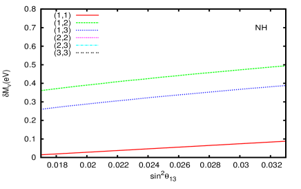
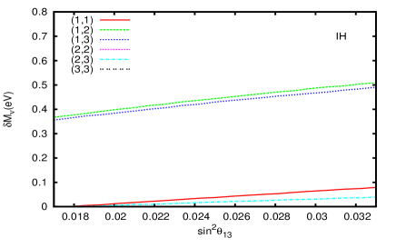
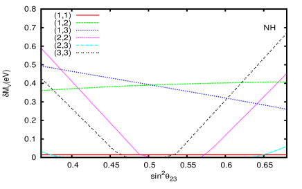
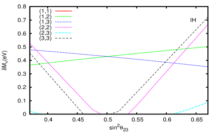
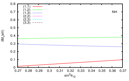
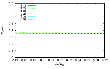
Figure 4: $(\delta M_{\nu}(i,j)\times 10^{2})$ as function of mixing angles for $m_{0}=0$ in case of NH (left) and IH (right) of neutrino mass matrix.

The dependency of $\delta M_{\nu}(1,2)$ and $\delta M_{\nu}(1,3)$ elements on $\theta_{13}$ and $\theta_{23}$ can be understood from the following analytical approximation. In case of NH, $m_{0}\equiv m_{1}\to 0$. Hence we have $m_{3}=\sqrt{\Delta m^{2}_{\rm atm}}$ and $m_{2}=\sqrt{\Delta m^{2}_{\odot}}$. As a result from Eq. (27) we get

$$|\delta M_{\nu}(1,2)| = \left[(s_{12}c_{13}(c_{12}c_{23}-s_{12}s_{23}s_{13})-1/3)\sqrt{\Delta m^{2}_{\odot}}+s_{13}c_{13}s_{23}\sqrt{\Delta m^{2}_{\rm atm}}\right]\,{\rm Exp}[-m_{0}/a]$$

$$|\delta M_{\nu}(1,3)| = \left[(s_{12}c_{13}(-c_{12}s_{23}-s_{12}c_{23}s_{13})+1/3)\sqrt{\Delta m^{2}_{\odot}}+s_{13}c_{13}c_{23}\sqrt{\Delta m^{2}_{\rm atm}}\right]\,{\rm Exp}[-m_{0}/a]$$ (59)

where the exponential factor in $|\delta M_{\nu}(1,2)|$ and $|\delta M_{\nu}(1,3)|$ gives the lightest neutrino mass dependency. Because of the cancellation, the 1st term in the square bracket is always suppressed in comparison to the second term. Therefore, we get:

$$|\delta M_{\nu}(1,2)| \approx \sqrt{\Delta m^{2}_{\rm atm}}\sin\theta_{13}\cos\theta_{13}\sin\theta_{23}\,{\rm Exp}[-m_{0}/a]$$

$$|\delta M_{\nu}(1,3)| \approx \sqrt{\Delta m^{2}_{\rm atm}}\sin\theta_{13}\cos\theta_{13}\cos\theta_{23}\,{\rm Exp}[-m_{0}/a]\,.$$ (60)

On the other hand in case of IH, $m_{0}\equiv m_{3}\to 0$. Hence we have $m_{2}\approx m_{1}=\sqrt{\Delta m^{2}_{\rm atm}}$. As a result, in the same analogy of Eq. (60), we get

$$|\delta M_{\nu}(1,2)| \approx \sqrt{\Delta m^{2}_{\rm atm}}\sin\theta_{13}\cos\theta_{13}\sin\theta_{23}\,{\rm Exp}[-m_{0}/a]$$

$$|\delta M_{\nu}(1,3)| \approx \sqrt{\Delta m^{2}_{\rm atm}}\sin\theta_{13}\cos\theta_{13}\cos\theta_{23}\,{\rm Exp}[-m_{0}/a]\,.$$ (61)

Thus in either cases the dependency of $\delta M_{\nu}(1,2)$ and $\delta M_{\nu}(1,3)$ elements on $\theta_{13}$ and $\theta_{23}$ are very similar. This can be checked from Fig. 4. It is evident from Fig. 4 that $\delta M_{\nu}(2,2)$, $\delta M_{\nu}(2,3)$, and $\delta M_{\nu}(3,3)$ elements don’t depend on $\theta_{12}$. Those elements depend mostly on the value of $\theta_{23}$. To understand this feature quantitatively, we write down the matrix elements $\delta M_{\nu}(2,2)$, $\delta M_{\nu}(2,3)$, and $\delta M_{\nu}(3,3)$ in the following. For normal ordering of the neutrino mass spectrum, we have $m_{0}\equiv m_{1}\to 0$. As a result, in the same analogy of Eq. (60), we have:

$$\delta M_{\nu}(2,2) \approx (\cos^{2}\theta_{13}\,\sin^{2}\theta_{23}-\frac{1}{2})\,\sqrt{\Delta m^{2}_{\rm atm}}\,{\rm Exp}[-m_{0}/a]\,,$$

$$\delta M_{\nu}(2,3) \approx (\sin\theta_{23}\,\cos\theta_{23}\,\cos^{2}\theta_{13}-\frac{1}{2})\,\sqrt{\Delta m^{2}_{\rm atm}}\,{\rm Exp}[-m_{0}/a]\,,$$

$$\delta M_{\nu}(3,3) \approx (\cos^{2}\theta_{13}\,\cos^{2}\theta_{23}-\frac{1}{2})\,\sqrt{\Delta m^{2}_{\rm atm}}\,{\rm Exp}[-m_{0}/a]$$ (62)

Clearly, $\delta M_{\nu}(2,2)$, $\delta M_{\nu}(2,3)$, and $\delta M_{\nu}(3,3)$ don’t depend on $\theta_{12}$ at all. There is a $\theta_{13}$ dependency and is of similar order if $\theta_{23}$ is near to its TBM value. However, once the value of $\theta_{23}$ deviates away from its TBM value, all these matrix elements mainly depend on the value of $\theta_{23}$. Moreover, all these $\delta M_{\nu}(i,j)$ increases as we move away from the TBM value. In case of IH, $m_{0}\equiv m_{3}\to 0$ and a similar pattern for all the $\delta M_{\nu}(i,j)$ is expected. This can be easily read from the right panel of Fig. 4.

III Application to Top-down approach

Now that we know the perturbed matrix from the bottom-up approach, we wish to construct models of neutrino masses and mixings in a top-down approach and elucidate the role of lightest neutrino mass. Our main objective here is that we will use the predictions of bottom-up approach as guide lines for building neutrino mass matrix whose tree-level mixing is governed by a symmetry. We then modify this using some perturbation so that the resulting values are consistent with the results that are obtained using the bottom up approach of section. II.2. We begin by proposing a model where the neutrino mixing is described by $U_{M}=U_{0}\,V$, where $V$ is the perturbed mixing matrix around the tree-level value and in general is given by:

$$V=V(1,2)\,V(1,3)\,V(2,3)\,,$$ (63)

with $V(i,j)$ being given by an orthogonal rotation matrix in the $(i,j)$ plane of neutrino mass matrix. Let us write down $V(i,j)$ explicitly such that the perturbed mixing matrix is

$$V=V(1,2)\,V(1,3)\,V(2,3) = \left(\begin{array}[]{ccc}1&\beta&0\\ -\beta&1&0\\ 0&0&1\end{array}\right)\left(\begin{array}[]{ccc}1&0&\alpha\\ 0&1&0\\ -\alpha&0&1\end{array}\right)\left(\begin{array}[]{ccc}1&0&0\\ 0&1&\gamma\\ 0&-\gamma&1\end{array}\right)$$ (77)

$$=\left(\begin{array}[]{ccc}1&\beta-\alpha\gamma&\alpha+\beta\gamma\\ -\beta&1&\gamma-\beta\alpha\\ -\alpha&-\gamma&1\end{array}\right),$$

where the determinant of $V(i,j)$ matrix is assumed to be unity. Since $U_{M}$ is the diagonalising matrix of the proposed neutrino mass matrix, we get

$$M_{\nu}^{D} = U^{T}_{M}\,(M_{\nu})_{M}\,U_{M}=U^{T}_{M}\,((M_{\nu})_{0}+\delta M_{\nu})\,U_{M}$$ (78)

$$=V^{T}\,U^{T}_{0}\,((M_{\nu})_{0}+\delta M_{\nu})\,U_{0}\,V\,,$$

where, $(M_{\nu})_{M}$ is the mass matrix in a flavor basis where charged leptons are real and diagonal. We now define a matrix $X$ such that

$$X \equiv V\,M_{\nu}^{D}\,V^{T}=U^{T}_{0}\,((M_{\nu})_{0}+\delta M_{\nu})\,U_{0}\,,$$ (79)

where the right-hand-side is determined through the bottom-up approach for a specific value of $m_{0}$, where as the left-hand-side involves six parameters, namely $m_{0}$, $\Delta m_{\rm atm}^{2}$, $\Delta m_{\odot}^{2}$, $\alpha,\beta$ and $\gamma$. Note that for $m_{0}<10^{-3}{\rm eV}$ we can neglect $m_{0}$ dependency as we discussed earlier in Section. II.2.

III.1 Application to Tri-bi-maximal mixing

Let us identify the tree-level mixing matrix as a tri-bi-maximal one, predicted by certain symmetry, then $U_{0}=U_{\rm TBM}$. As a result from Eq. (79) we get

$$X \equiv V\,M_{\nu}^{D}\,V^{T}=U^{T}_{\rm TBM}\,((M_{\nu})_{\rm TBM}+\delta M_{\nu})\,U_{\rm TBM}\,.$$ (80)

The matrix elements $X(i,j)$ can be expressed in terms of $m_{1},\,m_{2},\,m_{3},\,\alpha,\,\beta,\,\gamma$ as

$$X(1,1)=m_{1}+m_{2}\,\beta^{2}+m_{3}\,\alpha^{2}\,,$$

$$X(1,2)=(m_{2}-m_{1})\,\beta+(m_{3}-m_{2})\alpha\,\gamma\,,$$

$$X(1,3)=(m_{3}-m_{1})\,\alpha\,+(m_{3}-m_{2})\beta\gamma\,,$$

$$X(2,2)=m_{1}\,\beta^{2}+m_{2}+m_{3}\,\gamma^{2}\,,$$

$$X(2,3)=-(m_{3}-m_{1})\,\alpha\,\beta\,+(m_{3}-m_{2})\gamma\,,$$

$$X(3,3)=m_{1}\,\alpha^{2}+m_{2}\gamma^{2}+m_{3}\,,$$ (81)

where $m_{2}=\sqrt{m_{1}^{2}+\Delta m_{\odot}^{2}}$ and $m_{3}=\sqrt{m_{1}^{2}+\Delta m_{\rm atm}^{2}}$, respectively. Here we assume normal ordering of the neutrino masses. We have ignored higher order terms in $\alpha,\,\beta,\,{\rm and}\,\gamma$. We wish to determine the range of $\alpha,\,\beta,\,\gamma$ such that $X(i,j)$ computed from Eq. (81) is compatible within the $3\sigma$ ranges of $X(i,j)$ derived from the bottom-up approach, i.e, from the right hand side of Eq. (80), for $m_{0}\equiv m_{1}=0$ (i.e., $m_{0}<10^{-3}$ eV) as well as for $m_{0}\equiv m_{1}\neq 0$ (i.e. $m_{0}>10^{-3}$ eV).

III.1.1 Case-I: $m_{0}\equiv m_{1}\to 0$

In Table. 2, we report all the elements of the matrix $X$ obtained using the bottom up approach for the TBM mixing scenario.

TBM	X(1,1)/eV	X(1,2)/eV	X(1,3)/eV	X(2,2)/eV	X(2,3)/eV	X(3,3)eV
Central values	$0.0203$	$0.0487$	$0.315$	$1.01$	$0.747$	$4.89$
$3\sigma$ range	$[0.87\times 10^{-4},0.269]$	$[-0.0937,0.118]$	$[0.0141,1.15]$	$[0.839,1.17]$	$[-0.153,1.05]$	$[4.57,5.14]$

Table 2: Values of $X(i,j)\times 10^{2}$ for TBM mixing from the bottom up approach for $m_{0}=0$.

We need to find the range of $\alpha$, $\beta$, and $\gamma$ so that $X(i,j)$ values computed from Eq. (81) are consistent with the values reported in Table. 2. We get the range of $\alpha$, $\beta$, and $\gamma$ by fitting $X(1,2)$, $X(1,3)$ and $X(2,2)$ in Eq. 81 with the corresponding $X(1,2)$, $X(1,3)$, and $X(2,2)$ ranges from Table. 2. Once the range of $\alpha$, $\beta$, and $\gamma$ are known, we then plug those in Eq. 81 to get the range of $X(1,1)$, $X(2,3)$, and $X(3,3)$ and are shown in Fig. 5.

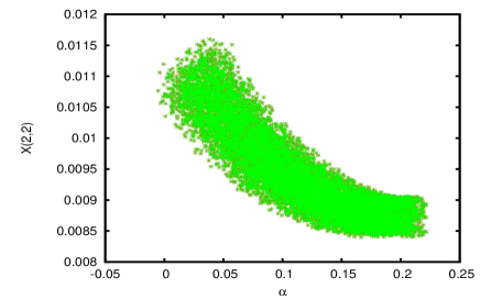
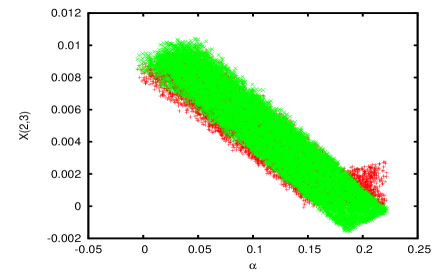
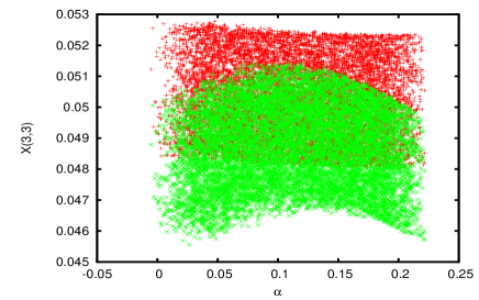
Figure 5: Range of $X(i,j)$ as a function of $\alpha$ for $\alpha,\,\beta,\,\gamma\neq 0$. The theory ranges are denoted by red whereas the experimental ranges from the bottom up approach are denoted by green.

Since $\alpha$, $\beta$ and $\gamma$ are non-zero, it is obvious that all the six $X(i,j)$ elements can be fitted within their experimental ranges. However, if more parameters are set to zero then it is not clear if all the six $X(i,j)$ elements can be fitted to their experimental values.

In order to realize the dependence of Eq. (81) on number of parameters, we analyze six different possibilities: Firstly, we set one of the three parameters to zero while keeping other two non zero (3 ways) and secondly, we set two of the three parameters to zero while keeping the third one non-zero (3 ways).

• First we set $\gamma=0$ and find the range of $\alpha$ and $\beta$ by comparing $X(1,2)$ and $X(1,3)$ with their experimental values given in Table. 2. Then we check the consistency of remaining four elements and shown in Fig. 6. It is clear that, although, the resulting range of $X(i,j)$s are compatible within their $3\sigma$ ranges, we do not get a very good fit for $X(2,3)$ because $\gamma$ is a perturbation in the $(2,3)$ plane. This in turn can be understood from Eq. (81) by setting $m_{1}=0$ and $\gamma=0$. Since $X(2,3)\propto m_{3}\alpha\beta$ and $\alpha$ is required to be small from fitting with $X(1,3)$, it is clear that theoretical values of $X(2,3)$ has minimal overlap with its experimental range of values.

  

  

  

  

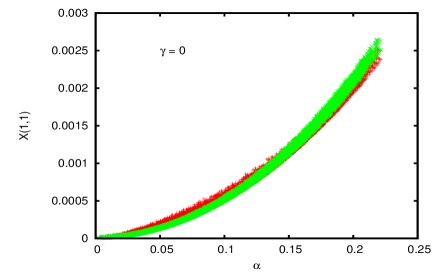
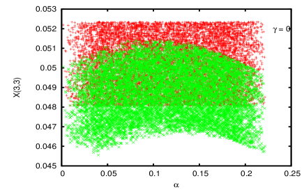
  Figure 6: Range of $X(i,j)$ as a function of $\alpha$ with $\gamma=0$. The theory ranges are denoted by red whereas the experimental ranges from the bottom up approach are denoted by green.

• We perform the same exercise by setting $\beta=0$. We fix the range of $\alpha$ and $\gamma$ from $X(1,3)$ and $X(2,2)$. Once the range of $\alpha$ and $\gamma$ are obtained, we then check the consistency of remaining four elements $X(1,1)$, $X(1,2)$, $X(2,3)$, $X(3,3)$. This is shown in Fig. 7. Since $\beta$ gives the perturbation in $(1,2)$ plane and the perturbations have minimal dependencies on $\beta$, we expect a better fit for all the elements. In fact this can be quickly checked from Eq. (81) by setting $m_{1}=0$ and $\beta=0$.

  

  

  

  

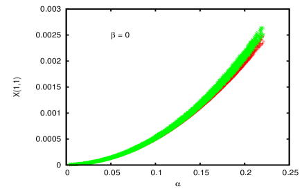
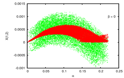
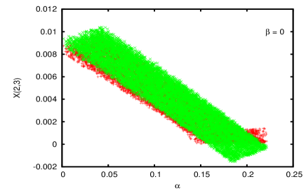
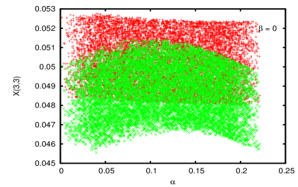
  Figure 7: Range of $X(i,j)$ as a function of $\alpha$ with $\beta=0$. The theory ranges are denoted by red whereas the experimental ranges from the bottom up approach are denoted by green.

• Next we set $\alpha=0$ and fix the range of $\beta$ and $\gamma$ from $X(1,2)$ and $X(2,2)$. Then we check the consistency of remaining four elements $X(1,1)$, $X(1,3)$, $X(2,3)$, $X(3,3)$ and are shown in Fig. 8. Since $\alpha$ is the perturbation in $(1,3)$ plane and it is set to zero, it is obvious that the theoretical values $X(1,3)$ has a minimal overlap with its $3\sigma$ range of experimental values. Note that $X(1,3)$ is not exactly zero even if $\alpha=0$. This in fact can be understood from Eq. (81) by setting $m_{1}=0$ and $\alpha=0$. In this limit $X(1,3)=(m_{3}-m_{2})\beta\gamma$ which is not zero. Thus we can get a required $\theta_{13}$ by doing perturbation in $(1,2)$ and $(2,3)$ plane.

  

  

  

  

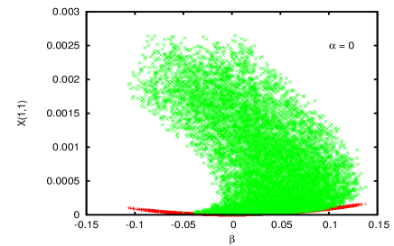
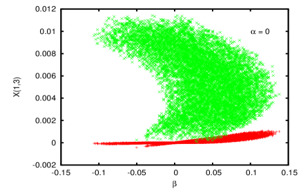
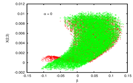
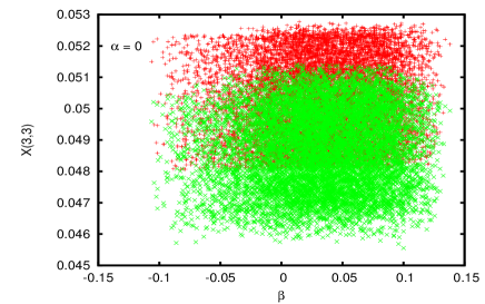
  Figure 8: Range of $X(i,j)$ as a function of $\beta$ for $\alpha=0$. The theory ranges are denoted by red whereas the experimental ranges from the bottom up approach are denoted by green.

Since we can set $\alpha$, $\beta$, and $\gamma$ to be zero individually, the order in which we do the rotations to construct the perturbed matrix $V$ is not very important. We further note that if $V$ is product of at least two matrices (that is $V$ is parameterized by at least two variables) then the parameters in $V$-matrix can not be considered as true-perturbation around their tree-level values. Therefore, the new parameters $\alpha,\beta,\gamma$… are arbitrary.

Now let us concentrate on the second case where we put two model parameters to zero while keeping third one to be non-zero. It is clear from Eq. (81) that setting either $(\alpha,\,\beta=0)$ or $(\alpha,\,\gamma=0)$ will give $X(1,3)=0$ which is not compatible with its $3\sigma$ range of experimental values reported in Table. 2. However, a non zero $\alpha$ with $(\beta,\,\gamma=0)$ is still a solution and is compatible with the experimental data set. In this case, we fix the range of $\alpha$ from $X(1,3)$ and check the consistency of remaining five elements. In the limit $m_{1}=0$ and $\beta=\gamma=0$, from Eq. (81) we see that $X(1,2)=X(2,3)=0$ and are compatible with their $3\sigma$ range of experimental values . The $\alpha$ dependency of remaining elements $X(1,1)$, $X(2,2)$, and $X(3,3)$ are shown in Fig. 9.

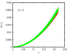
Figure 9: Range of $X(i,j)$ as a function of $\alpha$ for $(\beta,\,\gamma=0)$. The theory ranges are denoted by red whereas the experimental ranges from the bottom up approach are denoted by green.

III.1.2 Case-II: $m_{0}\equiv m_{1}>10^{-3}{\rm eV}$

Now we discuss the role of the non-zero lightest neutrino mass in determining the form of the perturbed matrix $V$. In Table. 3 and Table. 4, we report all the elements of the matrix $X$ for $m_{0}=0.01\,{\rm and}\,0.1\,{\rm eV}$ obtained using the bottom up approach for the TBM mixing scenario.

TBM	X(1,1)/eV	X(1,2)/eV	X(1,3)/eV	X(2,2)/eV	X(2,3)/eV	X(3,3)/eV
Central values	$1.02$	$0.044$	$0.26$	$1.45$	$0.68$	$5.00$
$3\sigma$ range	$[1.0,1.22]$	$[-0.054,0.086]$	$[0.0079,0.95]$	$[1.31,1.60]$	$[-0.15,0.96]$	$[4.68,5.26]$

Table 3: Values of $X(i,j)\times 10^{2}$ for TBM mixing from the bottom up approach for $m_{0}=0.01\,{\rm eV}$.

TBM	X(1,1)/eV	X(1,2)/eV	X(1,3)/eV	X(2,2)/eV	X(2,3)/eV	X(3,3)/eV
Central values	$10.0$	$0.013$	$0.075$	$10.08$	$0.21$	$11.16$
$3\sigma$ range	$[10.0,10.06]$	$[-0.0012,0.023]$	$[0.00028,0.28]$	$[10.03,10.11]$	$[-0.046,0.30]$	$[11.02,11.26]$

Table 4: Values of $X(i,j)\times 10^{2}$ for TBM mixing from the bottom up approach for $m_{0}=0.1\,{\rm eV}$.

To demonstrate the dependency of $X(i,j)$ on $m_{0}$ we consider only one out of six set of solutions discussed above. In particular, we choose the most non-trivial one with $\alpha=0$ and $\beta,\,\gamma\neq 0$. Because from Fig. 8 we see that, in this case, we can get the required values of $\theta_{13}$ even in the absence of perturbation in $(1,3)$ plane. We fix the range of $\beta$, $\gamma$ from the experimental values of $X(1,2)$ and $X(2,2)$ given in Table. 3 and Table. 4 for two different values of $m_{0}$. We then check the consistency of remaining four elements. It is evident from Fig. 8 that, in the limit $m_{0}=m_{1}\to 0$, the theoretical values of $X(1,3)$ has minimal overlapping with experimental values. Therefore, we choose this case to further study the dependency of $X(1,3)$ on non-zero values of $m_{0}$ and the result is shown in Fig. 10. It is clear that the fitting with the experimental data improves once we go from $m_{0}=0$ to non zero values of $m_{0}$.

We summarize our findings in Table. 5. It is clear from our analysis that any perturbation to the TBM mass matrix where two parameters are non zero can reproduce the experimental data. It is not necessary to have perturbation in $(1,3)$ plane to reproduce the experimental data as frequently discussed in the literature. Perturbations in $(1,2)$ and $(2,3)$ plane are equally good to get a reasonable fit within $3\sigma$ of the experimental data. However, once we set two parameters in $(1,2)$ and $(2,3)$ plane to zero, then perturbation along the $(1,3)$ plane is necessary to get compatible results with the experimental data.

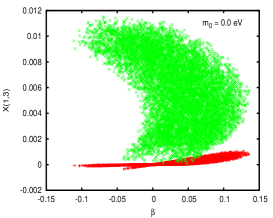
Figure 10: Range of $X(1,3)$ as a function of $\beta$ for $\alpha=0$ at $m_{0}=0.0,\,0.01,\,0.1\,{\rm eV}$, respectively. The theory ranges are denoted by red whereas the experimental ranges from the bottom up approach are denoted by green.

$\alpha=0$	$\beta,\,\gamma\neq 0$	$\surd$
$\beta=0$	$\alpha,\,\gamma\neq 0$	$\surd$
$\gamma=0$	$\alpha,\,\beta\neq 0$	$\surd$
$\alpha,\,\beta=0$	$\gamma\neq 0$	$\times$
$\alpha,\,\gamma=0$	$\beta\neq 0$	$\times$
$\gamma,\,\beta=0$	$\alpha\neq 0$	$\surd$

Table 5: Six different possibilities out of which four are consistent with data. These are true irrespective of the value of the lightest neutrino mass $m_{0}$.

IV Conclusion

The large value of $\theta_{13}$ predicted by Daya Bay and RENO put a stringent constraint on theoretical model buildings for neutrino mixing. All the well known mixing ansatzs such as TBM mixing, BM mixing, and DC mixing predict $\theta_{13}$ to be zero and hence not consistent with experiment. However, a lot of phenomenological models in the top-down scenario have been proposed in order to explain the non zero $\theta_{13}$, where a large value of the 1-3 mixing angle $\theta_{13}$ is generated through a perturbation to these mixing scenarios. In this paper we propose a perturbative bottom-up approach to quantify accurately the perturbation required for each element around a tree level mass matrix that is determined using the TBM mixing ansatz. Using the inputs from bottom-up approach we propose a model for neutrino masses and mixings. Though we used TBM mixing as an example, our analysis is more general and can be applied to any other ansatz which predicts $\theta_{13}=0$ at the tree-level.

We first summarize our results for the bottom-up approach:

• It is known that in a flavor basis the elements of the neutrino mass matrix can be written in terms of the oscillation parameters and the absolute value of lightest neutrino mass ($m_{0}$). In this context we point out that for $m_{0}\ll 10^{-3}\,{\rm eV}$, the perturbed elements don’t depend on the value of $m_{0}$. Therefore, all the perturbed elements can be determined exactly in terms of the oscillation parameters. However, in the opposite limit, where $m_{0}\mbox{\raisebox{-2.58334pt}{~{}$\stackrel{{\scriptstyle>}}{{\sim}}$~{}}}10^{-3}\,{\rm eV}$, we find that the perturbed elements have exponential dependency on the value of $m_{0}$. We factor out the $m_{0}$ dependency of all $\delta M_{\nu}(i,j)$ using an exponential parameterization as given in Eq. (28). This helps us in determining the exact dependency of the perturbed matrix elements on the value of $\theta_{13}$, $\theta_{23}$ and $\theta_{12}$ for all values of $m_{0}$.

• In order to gauge the size of the perturbation to each element of the mass matrix, we first compare the perturbed matrix elements with the corresponding tree level mass matrix derived from the TBM mixing ansatz and find that only the $(1,2)$ and $(1,3)$ elements needs to be significantly modified to be consistent with the experimental data. This is true for normal as well as inverted ordering of the neutrino mass spectrum.

• We show the exact dependency of the perturbed matrix elements on the value of $\theta_{13}$, $\theta_{23}$ and $\theta_{12}$. We find that $(1,1)$, $(1,2)$ and $(1,3)$ elements of the perturbed matrix do depend on all the three mixing angles. However, their dependency on $\theta_{12}$ is quite small as compared to that of $\theta_{13}$ and $\theta_{23}$. This, in act, is true for normal as well as inverted hierarchy of the neutrino mass spectrum. However, the $(2,2)$, $(2,3)$, and $(3,3)$ elements depend only on the value of $\theta_{23}$. Similar conclusions can be drawn for inverted hierarchy as well.

We use the results of bottom-up approach as guide-lines for determining a perturbative model of neutrino masses and mixings. We introduce a typical mixing matrix $U_{M}=U_{\rm TBM}\,V$ for the neutrino mass matrix, where $V(\alpha,\beta,\gamma)$ is the perturbed mixing matrix. We fix the parameters $\alpha$, $\beta$, and $\gamma$ from the oscillation data obtained using the bottom up approach, where $\alpha$, $\beta$ and $\gamma$ are the rotation angles in (1,3), (1,2) and (2,3) planes respectively. Here are some important observations from our top down analysis.

• We find that we can set any one parameter to zero, i.e, $(\alpha,\,\beta,\,{\rm or}\,\gamma=0)$ and still get a reasonably good fit with the experimental data that are derived using the bottom up approach. Although, keeping $\beta=0$ and $\alpha,\,\gamma\neq 0$ gives a much better fit, it is worth mentioning that $\alpha=0$ and $\beta,\,\gamma\neq 0$ also gives a reasonably good fit with the experimental data set. Thus, it is not necessary to have a perturbation in the $(1,3)$ plane in order to be compatible with the experimental data. This is one feature that was not explored in any earlier work.

• Once we set $(\alpha,\,\beta=0)$ or $(\alpha,\,\gamma=0)$, our results are not compatible within $3\sigma$ range of the experimental data. We, however, can set $\alpha\neq 0$ and $(\beta,\,\gamma=0)$ and still get a reasonably good fit with the experimental data. This case has been explored extensively in the literature.

• It is worth mentioning that the lightest neutrino mass plays an important role in the parameter fitting. The fitting improves once we go from a zero to non zero values of lightest neutrino mass. In particular for $m_{0}\mbox{\raisebox{-2.58334pt}{~{}$\stackrel{{\scriptstyle>}}{{\sim}}$~{}}}10^{-3}{\rm eV}$ we get large overlapings between the theoretical values of $X(i,j)$ with their experimental values.

• Since $\alpha$, $\beta$, and $\gamma$ can be set to zero separately, their ordering is not important. We further note that, if $V$ is parameterized by more than one variable then the perturbations are arbitrary. In other words, those can not be treated as true perturbations with respect to their tree level mixing angles.

- (1) B. Pontecorvo, Sov. Phys. JETP 7, 172 (1958) [Zh. Eksp. Teor. Fiz. 34, 247 (1957)]; B. Pontecorvo, Sov. Phys. JETP 26 (1968) 984–988; V. N. Gribov and B. Pontecorvo, Phys. Lett. B28 (1969) 493 .
- (2) Z. Maki, M. Nakagawa and S. Sakata, Prog. Theor. Phys. 28, 870 (1962) ; M. Kobayashi and T. Maskawa, Prog. Theor. Phys. 49 (1973) 652–657 .
- (3) S. M. Bilenky, J. Hosek, and S. T. Petcov, Phys. Lett. B94 (1980) 495 .
- (4) P. Langacker, S. T. Petcov, G. Steigman, and S. Toshev, Nucl. Phys. B282 (1987) 589 .
- (5) Q. R. Ahmad et al [SNO collaboration], Phys. Rev. Lett. 87, 071301 (2001) [arXiv:nucl-ex/0106015] .
- (6) K. Eguchi et al [KamLAND collaboration], Phys. Rev. Lett. 92, 071301 (2004) [arXiv:hep-ex/0310047] .
- (7) Y. Itow et al [T2K collaboration], [arXiv:hep-ex/0106019] .
- (8) D. S. Ayres et al [NOA collaboration], [arXiv:hep-ex/0503053] .
- (9) K. Abe et al. [T2K Collaboration], Phys. Rev. Lett. 107, 041801 (2011) [arXiv:1106.2822 [hep-ex]] .
- (10) P. Adamson et al. [MINOS Collaboration], Phys. Rev. Lett. 107, 181802 (2011) [arXiv:1108.0015 [hep-ex]] .
- (11) Y. Abe et al. (Double Chooz Collaboration), Phys. Rev. Lett. 108, 131801 (2012) .
- (12) F. P. An et al. [DAYA-BAY Collaboration], arXiv:1203.1669 [hep-ex] .
- (13) J. K. Ahn et al. [RENO Collaboration], arXiv:1204.0626 [hep-ex] .
- (14) T. Thummler [KATRIN Collaboration], arXiv:1012.2282 [hep-ex] .
- (15) C. L. Bennett, D. Larson, J. L. Weiland, N. Jarosik, G. Hinshaw, N. Odegard, K. M. Smith and R. S. Hill et al., arXiv:1212.5225 [astro-ph.CO] .
- (16) R. N. Mohapatra and W. Rodejohann, Phys. Rev. D 72, 053001 (2005) [hep-ph/0507312]; A. S. Joshipura and A. Y. .Smirnov, Nucl. Phys. B 750, 28 (2006) [hep-ph/0512024]; Z. -z. Xing, H. Zhang and S. Zhou, Phys. Lett. B 641, 189 (2006) [hep-ph/0607091];
- (17) H. Ishimori, T. Kobayashi, H. Ohki, Y. Omura, R. Takahashi and M. Tanimoto, Phys. Lett. B 662, 178 (2008) [arXiv:0802.2310 [hep-ph]].
- (18) R. N. Mohapatra, S. Nasri and H. -B. Yu, Phys. Lett. B 639, 318 (2006) [hep-ph/0605020].
- (19) C. Hagedorn, M. Lindner and R. N. Mohapatra, JHEP 0606, 042 (2006) [hep-ph/0602244]; C. S. Lam, Phys. Rev. Lett. 101, 121602 (2008) [arXiv:0804.2622 [hep-ph]]; F. Bazzocchi and S. Morisi, Phys. Rev. D 80, 096005 (2009) [arXiv:0811.0345 [hep-ph]] .
- (20) E. Ma and G. Rajasekaran, Phys. Rev. D 64, 113012 (2001) [hep-ph/0106291]; S. F. King and M. Malinsky, Phys. Lett. B 645, 351 (2007) [hep-ph/0610250]; G. Altarelli and F. Feruglio, Nucl. Phys. B 741, 215 (2006) [hep-ph/0512103]; M. Hirsch, A. S. Joshipura, S. Kaneko and J. W. F. Valle, Phys. Rev. Lett. 99, 151802 (2007) [hep-ph/0703046 [HEP-PH]]. B. Brahmachari, S. Choubey and M. Mitra, Phys. Rev. D 77, 073008 (2008) [Erratum-ibid. D 77, 119901 (2008)] [arXiv:0801.3554 [hep-ph]]; F. Feruglio, C. Hagedorn, Y. Lin and L. Merlo, Nucl. Phys. B 832, 251 (2010) [arXiv:0911.3874 [hep-ph]] .
- (21) H. Ishimori, T. Kobayashi, H. Ohki, Y. Shimizu, H. Okada and M. Tanimoto, Prog. Theor. Phys. Suppl. 183, 1 (2010) [arXiv:1003.3552 [hep-th]]; S. F. King and C. Luhn, Rept. Prog. Phys. 76, 056201 (2013) [arXiv:1301.1340 [hep-ph]]; G. Altarelli and F. Feruglio, New J. Phys. 6, 106 (2004) [hep-ph/0405048].
- (22) A. Dighe and N. Sahu, arXiv:0812.0695 [hep-ph]; G. Couture, C. Hamzaoui, S. S. Y. Lu and M. Toharia, Phys. Rev. D 81, 033010 (2010) [arXiv:0910.3132 [hep-ph]]; E. Bertuzzo, P. A. N. Machado and R. Z. Funchal, JHEP 1306, 097 (2013) [arXiv:1302.0653 [hep-ph]].
- (23) E. Ma, Phys. Rev. D 70, 031901 (2004) [hep-ph/0404199] ; P. F. Harrison, D. H. Perkins and W. G. Scott, Phys. Lett. B 530, 167 (2002) [hep-ph/0202074] ; Z. -z. Xing, Phys. Lett. B 533, 85 (2002) [hep-ph/0204049] ; X. G. He and A. Zee, Phys. Lett. B 560, 87 (2003) [hep-ph/0301092] .
- (24) V. D. Barger, S. Pakvasa, T. J. Weiler and K. Whisnant, Phys. Lett. B 437, 107 (1998) [hep-ph/9806387] ; G. Altarelli and F. Feruglio, JHEP 9811, 021 (1998) [hep-ph/9809596] ; R. N. Mohapatra and S. Nussinov, Phys. Rev. D 60, 013002 (1999) [hep-ph/9809415] .
- (25) H. Fritzsch and Z. -Z. Xing, Phys. Lett. B 372, 265 (1996) [hep-ph/9509389] ; H. Fritzsch and Z. -z. Xing, Phys. Lett. B 440, 313 (1998) [hep-ph/9808272] .
- (26) D. V. Forero, M. Tortola and J. W. F. Valle, Phys. Rev. D 86, 073012 (2012) [arXiv:1205.4018 [hep-ph]] .
- (27) M. C. Gonzalez-Garcia, M. Maltoni, J. Salvado and T. Schwetz, [arXiv:1209.3023 [hep-ph]] .
- (28) B. Brahmachari and A. Raychaudhuri, Phys. Rev. D 86, 051302 (2012) [arXiv:1204.5619 [hep-ph]] ; X. -G. He and A. Zee, Phys. Rev. D 84, 053004 (2011) [arXiv:1106.4359 [hep-ph]] ; B. Grinstein and M. Trott, JHEP 1209, 005 (2012) [arXiv:1203.4410 [hep-ph]] ; S. F. King, Phys. Lett. B 659, 244 (2008) [arXiv:0710.0530 [hep-ph]] ; S. Boudjemaa and S. F. King, Phys. Rev. D 79, 033001 (2009) [arXiv:0808.2782 [hep-ph]] ; D. Meloni, F. Plentinger and W. Winter, Phys. Lett. B 699, 354 (2011) [arXiv:1012.1618 [hep-ph]] ; E. Ma and D. Wegman, Phys. Rev. Lett. 107, 061803 (2011) [arXiv:1106.4269 [hep-ph]] ; S. Gupta, A. S. Joshipura and K. M. Patel, Phys. Rev. D 85, 031903 (2012) [arXiv:1112.6113 [hep-ph]] ; E. Ma, Phys. Lett. B 660, 505 (2008) [arXiv:0709.0507 [hep-ph]] ; B. Adhikary, B. Brahmachari, A. Ghosal, E. Ma and M. K. Parida, Phys. Lett. B 638, 345 (2006) [hep-ph/0603059] ; E. Bertuzzo, P. A. N. Machado, R. Z. Funchal and , arXiv:1302.0653 [hep-ph] ; J. A. Acosta, A. Aranda, M. A. Buen-Abad, A. D. Rojas and , Phys. Lett. B 718, 1413 (2013) [arXiv:1207.6093 [hep-ph]] .