Photometric AGN reverberation mapping of 3C120

We present the results of a five month monitoring campaign of the local active galactic nuclei (AGN) 3C120. Observations with a median sampling of two days were conducted with the robotic 15cm telescope VYSOS-6 located near Cerro Armazones in Chile. Broad band ($B$,$V$) and narrow band (NB) filters were used in order to measure fluxes of the AGN and the H$\beta$ broad line region (BLR) emission line. The NB flux is constituted by about 50% continuum and 50% H$\beta$ emission line. To disentangle line and continuum flux, a synthetic H$\beta$ light curve was created by subtracting a scaled $V$-band light curve from the NB light curve. Here we show that the H$\beta$ emission line responds to continuum variations with a rest frame lag of $23.6\pm 1.69$ days. We estimate a virial mass of the central black hole $M_{\rm BH}=57\pm 27\cdot 10^{6}\,M_{\odot}$, by combining the obtained lag with the velocity dispersion of a single contemporaneous spectrum. Using the flux variation gradient (FVG) method, we determined the host galaxy subtracted rest frame 5100Å  luminosity at the time of our monitoring campaign with an uncertainty of 10% ($L_{\rm{AGN}}=(6.94\pm 0.71)\times 10^{43}erg\leavevmode\nobreak\ s^{-1}$). Compared with recent spectroscopic reverberation results, 3C120 shifts in the $R_{BLR}$ - $L_{AGN}$ diagram remarkably close to the theoretically expected relation of $R\propto L^{0.5}$. Our results demonstrate the performance of photometric AGN reverberation mapping, in particular for efficiently determining the BLR size and the AGN luminosity.

1 Introduction

Reverberation mapping (Blandford & McKee 1982), where spectroscopic monitoring is used to measure the response delay $\tau$ of the broad emission lines to nuclear continuum variations, has proven to be a powerful tool to measure the average distance of the BLR clouds to the central source $R_{\rm{BLR}}=\tau\cdot c$.

The spectroscopy provides us also with a velocity dispersion $\sigma_{\rm{v}}$ of the emitting gas. Then, adopting Keplerian motion, one may estimate the enclosed mass, dominated by the supermassive black hole (Peterson et al. 2004 and references therein).

From theoretical considerations (Netzer 1990), the relationship $R_{\rm{BLR}}\propto L_{\rm{AGN}}^{\alpha}$, between H$\beta$ BLR size and nuclear luminosity (5100Å), should have $\alpha=0.5$. This has been investigated intensively (Koratkar & Gaskell 1991; Kaspi et al. 2000, 2005; Bentz et al. 2006, 2009a), with the latest result being $\alpha=0.519^{+0.063}_{-0.066}$.

Notably a new technique for distance determination based on dust-reverberation mapping has been presented (Yoshii 2002). Modifying these concepts, it has recently been proposed that the $R_{\rm{BLR}}\propto L_{\rm{AGN}}^{\alpha}$ relationship can be used as an alternative luminosity distance indicator. The intrinsic luminosity of the AGN ($L_{\rm{AGN}}$) can be inferred from the radius of the BLR ($R_{\rm{BLR}}$), resulting in the determination of the AGN distance. Moreover, due to the large luminosity and the extensive range of redshift at which the AGNs can be observed, the $R_{\rm{BLR}}-L_{\rm{AGN}}$ relationship offers the opportunity to discriminate between different cosmologies and to probe the dark energy (Haas et al. 2011; Watson et al. 2011). However, these methods require that the large scatter of the current $R_{\rm{BLR}}-L_{\rm{AGN}}$ relation can be reduced significantly, i.e. by factors up to 10, and that reverberation mapping of large samples can be performed efficiently.

Recently, Haas et al. (2011) have revisited photometric reverberation mapping. They demonstrated for Ark120 and PG0003+199 (Mrk335) that this method is very efficient and even applicable using very small telescopes. Broad filters are used to measure the triggering continuum, while suitable narrow band filters catch the emission line response.

The estimation of the host-subtracted nuclear luminosity $L_{\rm{AGN}}$ is challenging as well. One may use high-resolution imaging data and model the host galaxy profile in order to disentangle the nuclear flux (Bentz et al. 2009a, using HST imaging). An alternative approach is provided by the flux variation gradient method (FVG, by Choloniewski 1981; Winkler 1997). This method can be easily applied to monitoring data and does not require high spatial resolution.

Table 1: Characteristics of 3C120

$\alpha$ (2000)(1)	$\delta$ (2000)(1)	z(1)	$D_{L}^{(2)}$	H$\beta lag^{(3)}$	$M_{BH}^{(3)}$	$A_{B}^{(4)}$	$A_{V}^{(4)}$
			(Mpc)	(days)	($M_{\odot}$)	(mag)	(mag)
04:33:11.095	+05:21:15.620	0.03301	145.0	38.5 ${}^{+21.3}_{-15.3}$	$55.5\pm 26.9\times 10^{6}$	1.283	0.986

,

3C120 is a nearby Seyfert 1 galaxy known to be strongly variable in the optical, characterized by short and long term variations with amplitudes of up to 2 mag on a timescale of 10 years (Lyutyi 1979; Webb et al. 1988). Subsequent studies showed amplitude variations of about 0.4 mag (Winkler 1997) and 1.5 mag (Sakata et al. 2010) on a timescale of 4 years monitoring. Furthermore, 3C120 was included in a complete eight years AGNs spectroscopic monitoring campaign conducted by Peterson et al. (1998a). Although 3C120 was a lower priority object (with 50 days average intervals between observations) the spectroscopic reverberation mapping results have shown that the H$\beta$ emission line time response allows one to determine the BLR size with an uncertainty of about 50% (Peterson et al. 2004). Through 3C120’s redshift of $z=0.0331$, the H$\beta$ line falls into the OIII filter at 5007Å. Consequently, it is an ideal candidate for our instrumentation, a robotic 15 cm refractor.

Here we present new measurements of the BLR size, host-subtracted AGN luminosity and black hole mass based on a well-sampled photometric reverberation mapping campaign, allowing us to revisit the position of 3C120 in the BLR size - luminosity relationship. As a lucky coincidence, Grier et al. (2012) have carefully monitored 3C120 spectroscopically one year after our campaign allowing us to directly compare our photometric monitoring results with their spectroscopic results.

Figure 1: CAFOS spectrum of 3C120 obtained on Oct.$27^{th}$ 2009. For illustration, the band passes of the filters used for the photometric monitoring are shaded (blue $B$-band, green $V$-band). The transmission of the narrow band ([OIII] 5007Å filter) is indicated by the red dotted line. While narrow band catches the redshifted H$\beta$ line, its flux is composed of about 50% H$\beta$ line (red shaded) and 50% the continuum (black shaded). Note that for actual flux calculations the filter curves are convolved with the transmission curve of the Alta U16 CCD camera.

2 Observations and data reduction

The photometric monitoring campaign was conducted between October 2009 and March 2010 using the robotic 15 cm VYSOS-6 telescope of the Universitätssternwarte Bochum, located near Cerro Armazones in Chile

The images were reduced using IRAF packages and custom written tools, following the standard procedures for image reduction. Light curves were obtained with a median sampling of 2 days in the $B$-band (Johnson band pass = $4330\pm 500$ Å), $V$-band (Johnson band pass = $5500\pm 500$ Å) and the redshifted H$\beta$ (NB = $5007\pm 30$ Å) line. Photometry was performed using a 7$\aas@@fstack{\prime\prime}$5 aperture. The light curves are calculated relative to $\sim$ 20 nearby non-variables reference stars located on the same field, having similar brightness as the AGN. The absolute calibration was obtained using the measured fluxes of reference stars from SA095 field (Landolt 2009) observed on the same nights as the AGN.

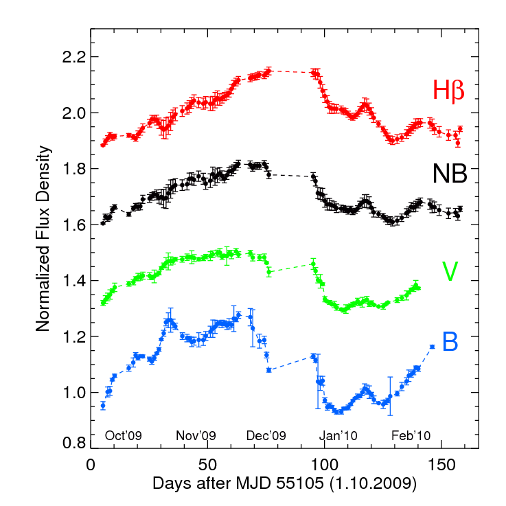
Figure 2: Observed light curves for 3C120 between Oct. 2009 and March 2010. The H$\beta$ light curve is computed by subtracting a scaled $V$ curve from the NB curve and re-normalizing it to mean $=1$. The light curves are vertically shifted by multiples of $0.2$ for clarity. The data gap between the end of December 2009 and the beginning of January 2010 is mostly due to strong wind preventing observations.

Additionally, we obtained an single epoch spectrum using the Calar Alto Faint Object Spectrograph (CAFOS) instrument at the 2.2 m telescope on Calar Alto observatory, Spain. The spectrograph’s slit width was 1$\aas@@fstack{\prime\prime}$54. The reduced spectrum is shown in Figure 1. 3C120 lies at redshift $z=0.0331$ so that the H$\beta$ line falls into the NB $5007\pm 30\AA$ filter. The NB filter effectively covers the line between velocities -3800km/s and +2200km/s. We determined that about 95% of the line flux is contained in the NB filter (red shaded line in Figure 1) through line profile deconvolution.

The characteristics of the source and a summary of the photometry results are listed in Table 1 and Table 2 respectively. Note that the magnitudes and the mean of the total flux have been corrected for galactic foreground extinction according to Schlegel et al. (1998). Observed fluxes in all bands are listed in Table 5.

3 Results and discussion

3.1 Light curves and BLR size

Table 2: Photometry results of 3C120

$B$	$V$	$OIII$	$fB_{total}^{(1)}$	$fV_{total}^{(1)}$	$fOIII_{total}^{(1)}$
(mag)	(mag)	(mag)	(mJy)	(mJy)	(mJy)
14.27-14.66	13.92-14.18	13.09-13.42	7.02$\pm$0.11	9.27$\pm$0.10	18.03$\pm$0.26

The light curves of 3C120 are shown in Figure 2. The $B$-band shows a gradual increase from the beginning of October to the beginning of December by 30%. Afterwards, the flux undergoes an abrupt drop by about 20% until mid-December 2009. Between the end of January and early February, the variability is more regular and the flux increases again to reach a third maximum at the end of February 2010. In contrast to the steep $B$ band flux increase, the narrow band (NB) flux increase is stretched until December 2009 to its first maximum. The sharp $B$ band flux decrease in December 2009, is reflected in the NB in early January 2010. Thus, at a first glance, the time delay of the H$\beta$ line against the continuum variations is 20 – 30 days.

Figure 3: Flux-flux diagram for the NB (OIII) and $V$ filter. Black dots denote the measurement pair of each night. The red and green lines represent the average flux in the OIII and $V$ band respectively. Fluxes were measured using circular 7.5” apertures. The data are as observed and not corrected for extinction.

As usual, the precise lag determination is done via cross correlation of light curves. However, as pointed out by Haas et al. (2011), the NB contains not only the emission line flux, but also a contribution of the varying continuum. Then cross correlating $B$ and NB, in principle, will result in two peaks, one peak from the emission line lag and one peak at zero lag from the auto-correlation of the continuum. These two peaks can only be discerned, if their separation is larger than the width of the auto-correlation. As illustrated in the top panel of Figure 4, in our case of 3C120 the two peaks are not separated, rather the $B/NB$ cross correlation shows only a very broad distribution. As proposed by Chelouche & Daniel (2012), one could try to disentangle the peaks in the correlation domain, for instance by subtracting a $B/V$ autocorrelation from the $B/NB$ cross correlation. But this requires a very precise normalization of the correlations. Therefore, we prefer a more straight forward approach by directly removing the continuum contribution from the NB light curve before applying the correlation techniques.

Figure 4: Cross correlation of $B$ and NB light curves (top) and of $B$ and H$\beta$ light curves (bottom). The dotted lines indicate the error range ($\pm 1\sigma$) around the cross correlation. The red shaded area marks the range used to calculate the centroid of the lag (vertical red dashed line).

From the spectrum we estimate that about 50% continuum and 50% H$\beta$ emission line contributes to the narrow band filter. The spectrum, however, was obtained with a much smaller aperture (slit width 1$\aas@@fstack{\prime\prime}$54) than the photometric light curves (7$\aas@@fstack{\prime\prime}$5 diameter). Moreover, we have only one single epoch spectrum, which does not allow us to easily determine the varying continuum contribution to the NB light curve. Therefore we consider the NB and V band light curves. Figure 3 shows for each night the narrow band (OIII) and $V$ band fluxes, calibrated to mJy. If the flux errors of each night are sufficiently small, then in principle one could subtract the $V$ band mJy light curve from the NB mJy light curve to obtain the H$\beta$ mJy light curve. However, our experience shows that this results in a rather noisy H$\beta$ light curve. Therefore, we used an average scaling of the NB and V band light curves, which turned out to yield good results. In fact, the results, i.e. the derived lags, do not depend sensitively on the precise choice of the average scaling factor.

The $V$ band flux, on average, corresponds to $\sim$ 56% of the narrow band flux (Fig. 3). Considering that the $V$ flux comprises the contributions from the continuum, the H$\beta$ and the OIII lines, our choice of 50% continuum flux in the NB is justifiable. Thus, we computed a synthetic H$\beta$ light curve by subtracting a scaled $V$ curve from the NB curve, i.e. H$\beta$ = NB $-$ 0.5 $V$.

We used the discrete correlation function (DCF, Edelson & Krolik 1988) to cross correlate the light curves. The cross correlation of $B$-band and H$\beta$ yields a time delay of 25.1 days defined by the centroid $\tau_{cent}$ (Fig. 4).

As usual we adopted the median sampling value (2 days) for the bin size in the DCF. In addition we checked whether the lag depends on the bin size. As discussed in detail by Rodriguez-Pascual et al. (1989), such dependencies could be caused by the scatter of the points in the light curves (bin size smaller than the median sampling) or by systematic noise structures (bin size grater than the median sampling). Figure 5 shows the lag as a function of bin size. Any deviation is clearly less than 2%, arguing in favour of our adopted bin size of 2 days.

Figure 5: Lag determined by the DCF versus bin size. The square symbol indicates the value used in this work (bin size of 2 days) and the dashed line represents the average value of 24.85. The data points are here connected by a line to guide the eye.

To determine the uncertainty in the time delay we applied the flux randomization and random subset selection method (FR/RSS, Peterson et al. 1998b, Peterson et al. 2004). From the observed light curves we create 2000 randomly selected subset light curves, each containing 63% of the original data. The flux value of each data point was randomly altered consistent with its (normal-distributed) measurement error. We calculated the discrete correlation function for the 2000 pairs of subset light curves and the corresponding centroid (Fig. 6). This yields a median lag $\tau_{cent}$ = 24.4 ${}^{+1.4}_{-2.1}$ days. Note the small lag uncertainty of less than 10%. Correcting for the time dilation factor we obtain a rest frame lag $\tau_{rest}$ = 23.6 $\pm 1.7$ days. This lag is somewhat smaller than the lag $\tau_{rest}$ = 27 $\pm 1$ days obtained by Grier et al. (2012), from their one year later spectroscopic reverberation mapping campaign. We will see below, that the lag difference nicely fits to the luminosity difference of 3C120 at the two campaigns (Sect. 3.1.3).

Figure 6: Results of the lag error analysis. The histogram shows the distribution of the centroid lag obtained by cross correlating 2000 flux randomized and randomly selected subset light curves (FR/RSS method). The red area marks the 68% confidence range used to calculate the errors of the centroid.

3.1.1 Virial mass of the central black hole

Using the velocity dispersion of the emitting gas together with the BLR size, it is possible to determine the mass of the central black hole following the virial theorem:

$${M_{BH}}=f\frac{R\cdot\sigma_{V}^{2}}{G}$$ (1)

where $\sigma_{V}$ is the emission-line velocity dispersion (assuming Keplerian orbits of the BLR clouds), $R=c\cdot\tau$ is the BLR size and the factor $f$ depends on the geometry and kinematics of the BLR (Peterson et al. 2004 and references therein). Most of the results presented in previous reverberation studies have been carried out considering only the virial product $c\tau\sigma_{V}^{2}/G$, ie. assuming a scaling factor $f=1$.

The first empirical calibration of the factor $f$ was obtained by Onken et al. (2004) who determined an average value of 5.5$\pm$1.8, assuming that AGNs and quiescent galaxies follow the same $M_{BH}-\sigma_{*}$ relationship. On the other hand, studies by Collin et al. (2006) show that the H$\beta$ profile is narrower in the rms spectra than in the mean spectra. Therefore, a higher velocity dispersion is expected in the mean spectra. Hence, they suggest a scaling factor $f=3.85$ (his table 2). Subsequents studies by Graham et al. (2011) (based on the method established by Onken et al. 2004) suggest a different scenario, reducing this first value to half (2.8$\pm$0.6). Therefore, the determination of the factor $f$ is an open issue involving theoretical models and empirical relationsh.png. Nevertheless, we here calculated the black hole mass ($M_{BH}$) adopting the value obtained by Onken et al. (2004), in order to compare our results with the literature.

Figure 7: CAFOS spectrum of 3C120, zoomed onto the H$\beta$ line. The solid black curve represents the spectrum after subtracting the narrow [OIII]$\lambda\lambda$4959,5007 emission lines (red dashed lines). The four dashed red lines (at the bottom of the H$\beta$ profile) show the narrow H$\beta$ models, for four intensities between 7% and 10% of the [OIII]$\lambda$5007 line. The four solid blue lines represent the spectrum after subtracting the narrow H$\beta$ models. Note that the broad faint HeII$\lambda$4686 emission line can be clearly seen, but its possible contribution to the H$\beta$ profile is negligible.

The velocity dispersion is determined from the width of the emission-line. It can be characterized by the second moment of the line profile ($\sigma_{\rm line}$) or by its full width at half maximum (FWHM). The first appears to be the most robust against measurement uncertainties (Peterson et al. 2004) and is widely used in subsequent reverberation studies. Usually - for spectroscopic monitoring data - the line dispersion $\sigma_{\rm line}$ is measured from the root-mean-square (rms) spectrum, in which the contribution of the narrow emission lines components disappears.

The feasibility of the use of single-epoch (SE) spectra for the black hole mass determination has been established in previous investigations (e.g. Vestergaard 2002, Woo et al. 2007, Denney et al. 2009a). On average, uncertainties of $\sim$30% have been reported for black hole mass determination from single epoch spectra measurements. However, the results of these studies have detected systematic sources of uncertainties, which arise mainly from the emission-line velocity dispersion and narrow line contamination (see Denney et al. 2009a, for details).

We here try to determine the black hole mass of 3C120 from our BLR size and the contemporaneous single epoch CAFOS spectrum.

The narrow emission lines [OIII]$\lambda\lambda$4959,5007 were modeled by single Gaussian profile and subtracted from the (SE) spectra (following Denney et al. 2009a). We also considered the theoretical intensity ratio for this doublet of 2.98 determined by Storey & Zeippen (2000) which is consistent with observational measurements and exhibit a negligible intensity variation (Dimitrijević et al. 2007). A challenge is to remove the narrow component of the H$\beta$ profile. Under the assumption of standard emission-line ratios, we model this contribution (following Denney et al. 2009a). The [OIII]$\lambda$5007 line profile was used to create the model of the narrow H$\beta$ emission, adopting a narrow H$\beta$ strength between 7% and 10% of the [OIII]$\lambda$5007 strength (following Woo et al. 2007). This narrow H$\beta$ model was then scaled and subtracted from the observed H$\beta$ line profile. Figure 7 shows the original H$\beta\lambda$4861 profile together with the narrow emission lines subtracted.

After removing the narrow H$\beta$ line (and the [OIII] lines), the H$\beta$ profile was isolated by the subtraction of a linear continuum fit, obtained through interpolation between two continuum segments on either end of the line, taking into account the possibility of local continuum contamination by FeII contribution and the red wing of the HeII$\lambda$4686 emission line (which may be blended with the blue wing of H$\beta$). Fig. 7 shows the original H$\beta\lambda$4861 profile together with the narrow emission lines subtracted. The velocity dispersion after removal of narrow lines is $\sigma_{\rm line}=1504\,km/s$.

From their recent spectroscopic reverberation campaign, Grier et al. (2012) determined $\sigma_{\rm line}(mean)=1687\pm 4\,km/s$ and $\sigma_{\rm line}(rms)=1514\pm 65\,km/s$. Note that in their mean spectra (their Fig. 1) the narrow H$\beta$ component appears stronger than in our spectrum, suggesting that our velocity dispersion may be underestimated. If true, this would be one of the possible systematic effects of single epoch spectra (Denney et al. 2009a). On the other hand, our time lag is about 40% smaller than the result derived by Peterson et al. (2004). Hence, according to photo-ionization physics, during our campaign the H$\beta$ region is closer to the ionizing source and in consequence higher velocities of the gas clouds are expected.

One shoud keep in mind that the black hole mass determination relies on the assumption that the BLR emitting gas clouds are in virialized motion. Although this has been shown for a large sample of AGNs, there are a few exceptions that have emerged as a fundamental limitation for black hole mass determination via reverberation mapping (e.g. Denney et al. 2009b, Gaskell 2010). Single epoch spectra can not identify such different velocity signatures of H$\beta$ clouds with a complex kinematical behavior.

Using the previous value (with 25% uncertainty adopted and our rest frame time lag $\tau=23.6$d, the virial black hole mass is $M_{virial}=(10\pm 5)\times 10^{6}M_{\odot}$ which is consistent, inside the margins of errors, with $M_{virial}=(12\pm 1)\times 10^{6}M_{\odot}$ derived by Grier et al. (2012) from their recent spectroscopic monitoring campaign and with $M_{virial}=(10\pm 5)\times 10^{6}M_{\odot}$ derived via spectroscopic reverberation mapping by Peterson et al. (2004). Considering the factor $f=5.5\pm 1.8$, we determine a central black hole mass $M_{BH}=(57\pm 27)\times 10^{6}M_{\odot}$.

3.1.2 Host-subtracted AGN luminosity

In order to determine the pure AGN luminosity, commonly at 5100Å, the contribution of the host galaxy to the nuclear flux has to be subtracted. The contribution of the host galaxy to the nuclear flux of 3C120 has been studied by Bentz et al. (2006, 2009a) using high resolution HST imaging as well as by Winkler et al. (1992), Winkler (1997) and Sakata et al. (2010) using the so-called flux variation gradient method, which was originally proposed by Choloniewski (1981). We here apply the FVG method to our 3C120 data and compare our results with the previous ones. Because the FVG method appears to be not widely known, we start with some comprehensive explanations here.

3.1.2.1 On the flux variation gradient method  

For multi-band AGN monitoring data, Choloniewski noticed a linear relationship between the fluxes obtained in two differents filters taken at different epochs. Using this relationship he demonstrated the existence of two component structure to the spectra of Seyfert galaxies. The two component structure assumes that one component (the host) is constant in time and that the second component (the AGN) has a strong variability. Despite of this strong variability the spectral energy distribution (SED) of the AGN does not change. Choloniewski plotted the observed UVB fluxes for 40 Seyfert galaxies as 3 dimensional vectors. This gave a clear geometrical interpretation of the total flux variations and allowed for the decomposition of the total vector flux $\@vec{\phi}(t)$ into a constant vector $\@vec{F}$ and a variable vector $\@vec{f}(t)$ (his figure 1).

Following the geometrical representation from Choloniewski (1981), is possible to write the two component structure using two different filters $(i,j)$ as:

$${\@vec{\phi}_{i,j}(\nu,t)}={\@vec{F}_{i,j}(\nu)}+{\@vec{f}_{i,j}(\nu,t)}$$ (2)

where the observed flux $\@vec{F}_{i,j}(\nu)$ and $\@vec{f}_{i,j}(\nu,t)$ are the constant and variable components in two arbitrary filters respectively.

With the - at optical wavelengths observationally corroborated - assumption that the shape of spectrum of the variable component does not change, one deduces:

$${{\@vec{f}_{j}(\nu,t)\over\@vec{f}_{i}(\nu,t)}}=a_{ji}$$ (3)

where $a_{ji}$ is a constant. Using equations (2) and (3) one obtains the equation of a straight line in the plane ($\@vec{\phi}_{i}$, $\@vec{\phi}_{j}$):

$${\@vec{\phi}_{j}(\nu,t)}={a_{ji}}{\@vec{\phi}_{i}(\nu,t)}+{b_{ji}}$$ (4)

where ${b_{ji}}$ = ${\@vec{F}_{j}(\nu)}-{a_{ji}}{\@vec{F}_{i}(\nu)}$

Thus the coefficient $a_{ji}$ represents the color index of the variable component. This coefficient of proportionality has also been called the flux variation gradient (FVG). It is denoted by the symbol $\Gamma$ by Winkler et al. (1992). Both, $a_{ji}$ and $b_{ji}$ coefficients have to be determined by a linear regression analysis.

The choice of which regression method to use depends on the degree of knowledge about the data, especially on how well separated the dependent and independent variables are, the measurement errors, the intrinsic dispersion of data around the best fit and others factors (see Isobe et al. 1990, for details).

Figure 8: Flux variation gradient diagram of 3C120. The solid lines delineate the bisector regression model yielding the range of the AGN slope. The dashed lines indicate the range of host slopes determined by Sakata et al. (2010) for 11 nearby AGN. The intersection between the host galaxy and AGN slope (red area) gives the host galaxy flux in both bands. The two vertical dotted and dashed lines show the host flux determined by Bentz et al. (2006) and Bentz et al. (2009a) respectively. The solid line shows the host flux obtained by Sakata et al. (2010). The dash-dotted blue lines represent the range of the AGN flux in both filters. Fluxes (black dots) were measured in a 7.5” aperture photometry and corrected for galactic foreground extinction.

Winkler et al. (1992) proposed a new method to separate the nuclear flux from the host galaxy, based on the flux-flux diagrams by Choloniewski (1981). Winkler et al. monitored 35 southern Seyfert galaxies using UBVRI multi-aperture photometry to estimate the colors of the host galaxy. They plotted the total fluxes obtained through 20^′′ and 30^′′ apertures, together with a line representing the fluxes from a component having the same colors as the host galaxy. The intersection of this line with the linear regression fit obtained from the total flux represents then the contribution from the host galaxy. As the observed source varies in luminosity, the fluxes in the FVG diagram will follow a slope representing the AGN color while the host will show no variation. The nuclear flux is then calculated by subtracting the constant host galaxy component (obtained by the FVGs method) from the total flux.

The studies by Choloniewski (1981) and Winkler et al. (1992) observationally established at optical wavelengths like in the BVRI bands that the AGN and host colors, i.e. flux ratios, are different but stay constant with time. Although these results have been corroborated by numerous authors (e.g., Yoshii et al. 2003; Suganuma et al. 2006; Doroshenko et al. 2008; Sakata et al. 2010), they are still a matter of a debate. For a more extensive discussion we refer the reader to Sakata et al. 2010.

A valuable study on the determination of the nuclear flux contribution was conducted by Sakata et al. (2010), using both HST imaging and the FVG method. In this study the flux of the host galaxy was estimated for 11 nearby Seyfert galaxies and QSOs. These fluxes were measured in B, V and I bands by using surface brightness fitting to the high resolution Hubble Space Telescope (HST) images and from the MAGNUM observations. The authors find a well defined range for the host galaxy slope of $0.4<\Gamma^{host}_{BV}<0.53$, which corresponds to host galaxy colors of $0.8<B-V<1.1$. The results - in particular on 3C120 - obtained by Sakata et al. (2010) are consistent (within measurement errors) with those obtained by Winkler (1997), Bentz et al. (2006) and Bentz et al. (2009a).

3.1.2.2 Application to 3C120  

Figure 8 shows the $B$ and $V$ fluxes obtained during the same nights and through the same aperture in a flux-flux diagram. The host color range is taken from Sakata et al. (2010) and drawn from the origin of ordinates (dashed lines). For the varying AGN flux (black dots), we use linear regression in order to determine a range of possible AGN colors (solid thin lines). The cross-section of the host and AGN slope allows us now to split the superposition of fluxes in both filters. Note that the $B$ and $V$ fluxes have been corrected for galactic foreground extinction according to Schlegel et al. (1998).

In both filters, the total flux (AGN+Host) contains a contribution from the emission lines originating in the narrow line region (NLR). However, this contribution is less than 10% of the host galaxy flux in the $B$ and $V$ band (Sakata et al. 2010). We here define the host galaxy to include the NLR line contribution.

Flux Variations Gradients (FVGs) were evaluated by fitting a straight line to the data using five methods of linear regression; OLS(Y/X), OLS(X/Y), OLS bisector, Orthogonal regression and Reduced Major-Axis (RMA) were used, depending on the corresponding error treatment of each method. Our regression algorithms are based on the formulas of Isobe et al. (1990) (their Table 1) and the variance for each method was calculated using the same formulation. The statistics of each linear regression fit are listed in Table 3.

Table 3: Linear regression results.

Method	$a^{a}$	$\sigma_{a}$	$b^{b}$	$\sigma_{b}$
OLS(Y/X)	1.04	0.04	-2.60	0.53
OLS(X/Y)	1.21	0.05	-4.22	0.33
OLS Bisector	1.12	0.04	-3.38	0.39
Orthogonal Regression	1.13	0.05	-3.48	0.41
RMA	1.22	0.06	-4.18	0.49

The bisector linear regression line and the OLS(X/Y) method yields a linear gradient of $\Gamma_{BV}=1.12\pm 0.04$ and $\Gamma_{BV}=1.04\pm 0.04$ respectively. The results are consistent, within the uncertainties, with $\Gamma_{BV}=1.11\pm 0.02$ determined by Sakata et al. (2010) and $\Gamma_{BV}=1.02\pm 0.07$ obtained by Winkler (1997). While the uncertainties to the OLS bisector and OLS(Y/X) regression slopes are lower (about 4%). According to Isobe et al. (1990), the OLS bisector method is the most suitable in order to determine the underlying relationship between the variables and it was also considered in previous studies of FVG method by Winkler (1997). Therefore, we adopted the OLS bisector linear regression to define the range of AGN slope.

Averaging over the intersection area between the AGN and the host galaxy slopes, we obtain a mean host galaxy flux of $(2.17\pm 0.33)$ mJy in $B$ and $(4.58\pm 0.40)$ mJy in $V$. Our host galaxy flux derived with the FVG method is consistent with the values $f_{B}\approx{2.10}$ mJy and $f_{V}\approx{4.73}$ mJy obtained by Sakata et al. (2010). Note that one has to coadd the values of Tables 5 and 8 of Sakata et al., in order to include the flux contribution of the narrow lines ([OIII]$\lambda$4959, 5007, H$\beta$, H$\gamma$) to each filter.

We have also compared our results with those obtained by Bentz et al. (2006) and Bentz et al. (2009a) through modeling of the host galaxy profile (GALFIT, Peng et al. 2002) from the high-resolution HST images. On the nucleus-free image and through an aperture of $5\arcsec\times 7\aas@@fstack{\prime\prime}6$, Bentz et al. (2006) determined a rest-frame 5100Å  host-flux $F_{5100\AA\leavevmode\nobreak\ }$ =$1.82\times 10^{-15}ergs^{-1}cm^{-2}\AA^{-1}$. Using the color term factor from the HST-F550M filter to 5100Å (their Table 3) we deduced the flux for the F550M filter to be $F_{F550M}$ =$1.74\times 10^{-15}ergs^{-1}cm^{-2}\AA^{-1}$. This corresponds after exinction correction to $4.62mJy$. Moreover, considering the contribution of the narrow lines in the $V$-band ($1.235mJy$), determined by Sakata et al. (2010), the previous value translates to $5.86mJy$. In a subsequent investigation, Bentz et al. (2009a) determined a host galaxy flux of $0.78\times 10^{-15}ergs^{-1}cm^{-2}\AA^{-1}$, which after extinction correction and adding the contribution of the narrow lines yield a value of $3.31mJy$. The difference between the two results by Bentz et al. lies mainly in the type of model used for the decomposition of the galaxy. The first study considered a general Sersic function for modeling bulges (Bentz et al. 2006). The second study performed the modeling with variations and improvements to the original profile (Bentz et al. 2009a). Our value ($fV_{host}=4.58mJy$) falls exactly in the middle between both values, simply suggesting that our determination is consistent, within the error margins, with those determined by Bentz et al.

Figure 9: Interpolated rest frame flux at 5100Å  from $fB_{AGN}$ and $fV_{AGN}$ fluxes (black dots) for an AGN continuum with power law spectral shape ($F_{\nu}\propto\nu^{\alpha}$) (solid lines).

The AGN fluxes at the time of our monitoring can be determined by subtracting the host galaxy fluxes from the total fluxes. During our monitoring campaign, the total $B$ fluxes lie in the range between 5.81-8.39 mJy with a mean of $(7.02\pm 0.11)$ mJy. The total $V$ fluxes lie in the range between 8.17-10.38 mJy with a mean $(9.27\pm 0.11)$ mJy. The host galaxy subtracted average AGN fluxes and the host galaxy flux contribution of 3C120 are listed in Table 4.

Also listed in Table 4 are the interpolated rest frame $5100\AA\leavevmode\nobreak\$ fluxes and the monochromatic AGN luminosity $\lambda L_{\rm{\lambda(AGN)}}$ at $5100\AA\leavevmode\nobreak\$. The rest frame flux at 5100Å  was interpolated from the host-subtracted AGN fluxes in both bands, adopting for the interpolation that the AGN has a power law SED ($F_{\nu}\propto\nu^{\alpha}$) with an spectral index $\alpha=\log(fB_{AGN}/fV_{AGN})/\log(\nu_{B}/\nu_{V})$, where $\nu_{B}$ and $\nu_{V}$ are the effective frequencies in the B and V bands, respectively. The error was determined by interpolation between the ranges of the AGN fluxes $\pm\sigma$ in both filters, respectively, as illustrated in Fig. 9.

To determine the luminosity, we used the distance of 145 Mpc (Bentz et al. 2009a). This yields $L_{\rm{AGN}}=(6.94\pm 0.71)\times 10^{43}ergs^{-1}$. The AGN luminosity during our campaign is about half the mean value of $(12.40\pm 2.6)\times 10^{43}ergs^{-1}$ found by Bentz et al. (2009a) for their campaign about 15 years ago and slightly lower than the value $(9\pm 1)\times 10^{43}ergs^{-1}$ found by Grier et al. (2012) for their campaign one year after ours.

Figure 10: $R_{BLR}-L$ relationship from data of Bentz et al. (2009a) (black dots) with a fitted slope $\alpha=0.519$ (dotted line). The diagram is zoomed to contain the objects of this work (3C120, blue dot) and Haas et al. (2011) (Ark120 and PG0003, green dots). The blue arrows show the positional shift of the new measurements with respect to the previous ones from Bentz et al. (2009a). The red arrow shows the shift of 3C120 between our result and that obtained by Grier et al. (2012). The slope $\alpha$ of this shift is remarkably close to the theoretically expected value of $\alpha=0.5$. The original position of 3C120 by Bentz et al. is in the center of the plot and marked by the square surrounding the fat dot.

3.1.3 The BLR size - luminosity relationship

From spectroscopic reverberation mapping, the relationship between the H$\beta$ BLR size and the luminosity (5100Å) of the AGN $R_{{\rm BLR}}\propto L^{\alpha}$ has been established by Kaspi et al. (2000). Bentz et al. (2009a) determined an improved slope of $\alpha=$ 0.519${}^{0.063}_{-0.066}$ from several spectroscopic reverberation mapping campaigns.

Figure 10 shows the $R_{{\rm BLR}}$ and $L_{AGN}$ values obtained by Bentz et al. (2009a), the result for 3C120 obtained by Grier et al. (2012) and the two objects Ark120 and PG0003 studied with well sampled photometric reverberation mapping by Haas et al. (2011). While the relationship appears to be well defined, many objects have large uncertainties yet and/or lie quite off the regression line. Part of this may simply be due to the fact that AGN are complex objects, but part of the dispersion may be due to poor early reverberation data. We just note that the new position of both Ark120 and PG0003 lies closer to the regression line in Fig. 10.

For 3C120 we have now three positions in the R-L diagram: one from Peterson’s spectroscopic monitoring campaign in 1998, quite on the regression line but having large uncertainties presumably due to sparse sampling; one from the spectroscopic monitoring campaign in 2010/2011 by Grier et al. (2012); and one from our photometric monitoring campaign in 2009/2010. The last two campaigns both have a good time sampling and small uncertainties. The striking result from these two campaigns is that the slope between these positions of 3C120 is $\alpha=0.504$, hence dueing the brightness changes 3C120 moves parallel to the theoretically expected slope (red arrow in Fig. 10). With increasing luminosity the BLR size grows proportional to the square root of the luminosity, and these changes appear to occur rather quickly, i.e. within days or weeks. However, this does not mean that the BLR gas clouds move that rapidly in- or outwards. Baldwin et al. (1995) have presented a model of locally optimally emitting clouds.

Table 4: Host galaxy subtracted AGN fluxes of 3C120

$fB_{host}$	$fB_{AGN}^{1}$	$fV_{host}$	$fV_{AGN}^{1}$	$f_{AGN}((1+z)5100$Å	$\lambda L_{\lambda,AGN}5100$Å
(mJy)	(mJy)	(mJy)	(mJy)	(mJy)	($10^{43}ergs^{-1}$)
2.17$\pm$0.33	4.85$\pm$0.35	4.58$\pm$0.40	4.68$\pm$0.41	4.72$\pm$0.40	6.94$\pm$0.71

It successfully explains the emission line characteristics of quasar spectra. This model provides also a nice explanation for the R-L relation. In the BLR the gas clouds actually populate a large range of radii, but, depending on the density and ionisation parameter, only at a suited narrow distance range (from the illuminating central power house) the gas clouds efficiently convert the nuclear continuum radiation into line emission. In this picture, a central continuum brightness variation can quickly change the BLR size proportional to $L^{0.5}$.

4 Summary and conclusions

Using a robotic 15 cm telescope located at an excellent site, we have performed a five months monitoring campaign for the Seyfert 1 galaxy 3C120. We determined the broad line region size, the virial black hole mass and the host-subtracted AGN luminosity. The results are:

1. The time lag $\tau_{rest}$ = 23.6 $\pm 1.69$ days, obtained from cross correlation of the H$\beta$ emission line with the optical continuum light curve, has changed over one decade, but the physical relation $R_{{\rm BLR}}\propto L_{{\rm AGN,\lambda 5100}}^{1/2}$ still holds. The small uncertainty in our measurements (7%) is presumably due to the well sampled photometric reverberation data.

2. The black hole mass $M_{BH}=57\pm 27\times 10^{6}M_{\odot}$ is consistent with the value of $55.5\pm 26.9\times 10^{6}M_{\odot}$ derived by Peterson et al. (2004) from spectroscopic reverberation mapping data and with the value of $M_{BH}=67\pm 6\times 10^{6}$ determined by Grier et al. (2012). However, the high uncertainties in the black hole mass, with respect to the most contemporaneus result, are attributed to the adopted 25% uncertainty for the line velocity dispersion and also considering the uncertainty introduced by the scale factor $f$.

3. Using the flux variation gradient method (FVG) and a conservatively limited host galaxy color range, it is possible to find the host galaxy subtracted AGN luminosity of 3C120 at the time of our monitoring campaign to be $L_{\rm{AGN}}=(6.94\pm 0.71)\times 10^{43}ergs^{-1}$.

The new results obtained for the BLR size and AGN luminosity of 3C120 fit well into the BLR size-luminosity diagram. We conclude that photometric reverberation mapping is an attractive method with the advantage to efficiently measure the BLR and the host-subtracted luminosities for large samples of quasars and AGNs. Not only applicable with small telescopes, photometric AGN reverberation mapping could become a key tool for the upcoming large monitoring campaigns, for instance with the Large Synoptic Survey Telescope (LSST). This could be an important step forward in order to constrain cosmologial parameters from the $R_{{\rm BLR}}\propto L_{{\rm AGN,\lambda 5100}}^{1/2}$ relationship in order to determine quasar distances and to probe the dark energy (Haas et al. 2011;Watson et al. 2011) as well as to enlarge the current statistics for black hole masses.

5

Table 5: $B$, $V$, $OIII$ and H$\beta$ Fluxes in mJy.

JD-2,450,000	$F_{B}$	$F_{V}$	$F_{OIII}$	$F_{H\beta}$
55110.250	$1.870\pm 0.032$	$3.443\pm 0.033$	$5.896\pm 0.018$	$4.174\pm 0.038$
55111.250	$-\pm-$	$3.487\pm 0.053$	$6.051\pm 0.060$	$4.308\pm 0.081$
55112.250	$1.978\pm 0.038$	$3.524\pm 0.051$	$6.009\pm 0.065$	$4.247\pm 0.083$
55113.238	$1.985\pm 0.034$	$3.555\pm 0.062$	$6.047\pm 0.069$	$4.269\pm 0.093$
55114.230	$2.074\pm 0.010$	$3.606\pm 0.027$	$6.216\pm 0.065$	$4.413\pm 0.070$
55115.230	$2.104\pm 0.012$	$3.653\pm 0.055$	$6.276\pm 0.054$	$4.450\pm 0.077$
55121.289	$2.165\pm 0.024$	$3.700\pm 0.031$	$6.108\pm 0.043$	$4.258\pm 0.053$
55123.211	$2.208\pm 0.035$	$3.721\pm 0.036$	$6.240\pm 0.055$	$4.379\pm 0.066$
55124.219	$2.265\pm 0.019$	$3.769\pm 0.026$	$6.299\pm 0.058$	$4.414\pm 0.064$
55125.219	$2.242\pm 0.014$	$3.789\pm 0.050$	$6.283\pm 0.080$	$4.388\pm 0.094$
55126.219	$2.257\pm 0.010$	$3.790\pm 0.042$	$6.293\pm 0.083$	$4.398\pm 0.093$
55127.270	$2.256\pm 0.011$	$3.808\pm 0.046$	$6.456\pm 0.096$	$4.552\pm 0.107$
55130.172	$2.235\pm 0.015$	$3.805\pm 0.043$	$6.475\pm 0.091$	$4.573\pm 0.100$
55131.180	$2.216\pm 0.022$	$3.786\pm 0.030$	$6.523\pm 0.088$	$4.629\pm 0.094$
55132.172	$2.245\pm 0.020$	$3.798\pm 0.084$	$6.569\pm 0.073$	$4.670\pm 0.112$
55133.211	$2.280\pm 0.008$	$3.824\pm 0.018$	$6.558\pm 0.116$	$4.646\pm 0.118$
55134.180	$2.311\pm 0.014$	$3.843\pm 0.024$	$6.487\pm 0.123$	$4.565\pm 0.126$
55135.180	$2.389\pm 0.006$	$3.911\pm 0.018$	$6.510\pm 0.176$	$4.555\pm 0.177$
55136.172	$2.438\pm 0.023$	$3.947\pm 0.029$	$6.471\pm 0.211$	$4.498\pm 0.213$
55137.191	$2.523\pm 0.027$	$3.980\pm 0.065$	$6.489\pm 0.245$	$4.498\pm 0.254$
55138.172	$2.539\pm 0.058$	$4.000\pm 0.111$	$6.595\pm 0.203$	$4.595\pm 0.232$
55139.172	$2.540\pm 0.094$	$4.005\pm 0.053$	$6.696\pm 0.212$	$4.693\pm 0.218$
55140.191	$2.513\pm 0.034$	$4.004\pm 0.038$	$6.750\pm 0.167$	$4.748\pm 0.171$
55141.191	$2.492\pm 0.024$	$4.028\pm 0.022$	$6.786\pm 0.149$	$4.771\pm 0.150$
55144.148	$2.415\pm 0.026$	$4.027\pm 0.038$	$6.788\pm 0.124$	$4.774\pm 0.130$
55146.191	$2.400\pm 0.029$	$4.055\pm 0.042$	$6.806\pm 0.129$	$4.778\pm 0.135$
55147.160	$2.394\pm 0.020$	$4.056\pm 0.024$	$6.930\pm 0.135$	$4.902\pm 0.137$
55148.180	$2.370\pm 0.036$	$4.054\pm 0.085$	$6.942\pm 0.132$	$4.915\pm 0.157$
55149.191	$2.375\pm 0.031$	$4.042\pm 0.045$	$6.912\pm 0.131$	$4.891\pm 0.139$
55151.180	$2.386\pm 0.056$	$4.028\pm 0.021$	$6.994\pm 0.120$	$4.980\pm 0.122$
55153.160	$2.385\pm 0.042$	$4.041\pm 0.032$	$6.935\pm 0.129$	$4.914\pm 0.133$
55154.180	$2.416\pm 0.034$	$4.064\pm 0.028$	$6.820\pm 0.131$	$4.788\pm 0.134$
55156.141	$2.449\pm 0.043$	$4.069\pm 0.059$	$6.892\pm 0.159$	$4.857\pm 0.170$
55157.180	$2.473\pm 0.068$	$4.095\pm 0.045$	$7.043\pm 0.164$	$4.995\pm 0.170$
55158.180	$2.488\pm 0.052$	$-\pm-$	$6.962\pm 0.179$	$4.915\pm 0.183$
55159.160	$2.511\pm 0.024$	$4.111\pm 0.038$	$7.013\pm 0.167$	$4.957\pm 0.176$
55160.230	$2.516\pm 0.015$	$4.116\pm 0.055$	$7.063\pm 0.134$	$5.004\pm 0.138$
55161.160	$2.510\pm 0.029$	$4.061\pm 0.034$	$7.007\pm 0.111$	$4.977\pm 0.112$
55162.148	$2.516\pm 0.020$	$4.073\pm 0.012$	$6.937\pm 0.095$	$4.900\pm 0.155$
55163.211	$2.497\pm 0.030$	$4.070\pm 0.122$	$7.016\pm 0.097$	$4.980\pm 0.103$
55164.160	$2.512\pm 0.039$	$4.110\pm 0.036$	$7.108\pm 0.094$	$5.053\pm 0.109$
55165.172	$2.505\pm 0.023$	$4.090\pm 0.055$	$7.116\pm 0.110$	$5.071\pm 0.116$
55166.148	$2.552\pm 0.101$	$-\pm-$	$7.158\pm 0.100$	$5.112\pm 0.107$
55167.141	$2.546\pm 0.018$	$4.132\pm 0.038$	$7.226\pm 0.090$	$5.159\pm 0.098$
55168.180	$2.581\pm 0.025$	$4.090\pm 0.038$	$7.281\pm 0.086$	$5.235\pm 0.097$
55173.180	$2.564\pm 0.067$	$4.109\pm 0.036$	$7.265\pm 0.083$	$5.211\pm 0.092$
55174.262	$2.477\pm 0.144$	$4.051\pm 0.045$	$7.188\pm 0.076$	$5.163\pm 0.088$
55175.172	$-\pm-$	$-\pm-$	$7.235\pm 0.068$	$5.210\pm 0.070$
55176.219	$-\pm-$	$-\pm-$	$7.233\pm 0.078$	$5.208\pm 0.101$
55177.180	$2.376\pm 0.055$	$4.051\pm 0.038$	$7.235\pm 0.073$	$5.209\pm 0.103$
55179.199	$2.384\pm 0.029$	$4.053\pm 0.044$	$7.281\pm 0.078$	$5.254\pm 0.091$
55180.180	$2.266\pm 0.022$	$3.979\pm 0.012$	$7.199\pm 0.087$	$5.210\pm 0.094$
55181.180	$2.147\pm 0.015$	$3.857\pm 0.064$	$7.028\pm 0.091$	$5.099\pm 0.128$
55200.160	$2.258\pm 0.019$	$3.910\pm 0.072$	$6.988\pm 0.090$	$5.033\pm 0.092$
55201.141	$2.226\pm 0.017$	$3.815\pm 0.046$	$6.880\pm 0.112$	$4.972\pm 0.118$
55202.160	$2.059\pm 0.213$	$3.693\pm 0.036$	$6.602\pm 0.130$	$4.755\pm 0.130$
55203.141	$2.045\pm 0.056$	$3.677\pm 0.089$	$6.586\pm 0.135$	$4.748\pm 0.137$
55204.172	$2.065\pm 0.034$	$3.639\pm 0.017$	$6.563\pm 0.148$	$4.744\pm 0.148$
55205.129	$1.912\pm 0.019$	$3.494\pm 0.035$	$6.420\pm 0.149$	$4.673\pm 0.156$
55206.148	$1.858\pm 0.022$	$3.463\pm 0.008$	$6.340\pm 0.134$	$4.608\pm 0.139$
55207.141	$1.869\pm 0.020$	$3.450\pm 0.025$	$6.342\pm 0.135$	$4.617\pm 0.136$
55208.141	$1.860\pm 0.011$	$3.425\pm 0.007$	$6.315\pm 0.116$	$4.602\pm 0.119$
55209.148	$1.834\pm 0.015$	$3.421\pm 0.043$	$6.299\pm 0.100$	$4.588\pm 0.115$
55210.148	$1.819\pm 0.015$	$3.383\pm 0.037$	$6.250\pm 0.101$	$4.559\pm 0.105$
55212.129	$1.822\pm 0.017$	$3.357\pm 0.015$	$6.241\pm 0.081$	$4.562\pm 0.083$
55213.141	$1.847\pm 0.011$	$3.347\pm 0.025$	$6.239\pm 0.072$	$4.565\pm 0.077$
55214.129	$1.849\pm 0.010$	$3.361\pm 0.055$	$6.222\pm 0.072$	$4.541\pm 0.076$
55215.129	$1.856\pm 0.018$	$3.383\pm 0.029$	$6.179\pm 0.068$	$4.487\pm 0.078$
55216.141	$1.880\pm 0.008$	$3.409\pm 0.021$	$6.230\pm 0.066$	$4.526\pm 0.070$
55217.109	$1.908\pm 0.008$	$3.423\pm 0.027$	$6.162\pm 0.062$	$4.450\pm 0.090$
55218.109	$1.929\pm 0.007$	$3.436\pm 0.023$	$6.190\pm 0.058$	$4.472\pm 0.058$
55219.129	$1.941\pm 0.020$	$3.468\pm 0.037$	$6.242\pm 0.066$	$4.508\pm 0.080$
55220.109	$1.945\pm 0.012$	$3.434\pm 0.023$	$6.327\pm 0.084$	$4.610\pm 0.090$
55221.121	$1.974\pm 0.026$	$3.452\pm 0.065$	$6.381\pm 0.104$	$4.655\pm 0.108$
55222.121	$2.005\pm 0.035$	$3.474\pm 0.009$	$6.414\pm 0.148$	$4.677\pm 0.148$
55223.090	$1.995\pm 0.035$	$3.486\pm 0.045$	$6.414\pm 0.154$	$4.671\pm 0.154$
55224.102	$1.975\pm 0.049$	$3.431\pm 0.033$	$6.375\pm 0.139$	$4.660\pm 0.144$
55225.109	$1.956\pm 0.018$	$3.444\pm 0.027$	$6.259\pm 0.125$	$4.537\pm 0.125$
55226.090	$1.917\pm 0.030$	$3.418\pm 0.006$	$6.152\pm 0.107$	$4.443\pm 0.107$
55228.109	$1.890\pm 0.006$	$3.395\pm 0.004$	$6.113\pm 0.071$	$4.415\pm 0.078$
55230.078	$1.880\pm 0.032$	$3.397\pm 0.036$	$6.062\pm 0.063$	$4.363\pm 0.072$
55231.090	$1.897\pm 0.019$	$3.418\pm 0.010$	$6.005\pm 0.072$	$4.296\pm 0.093$
55232.078	$1.911\pm 0.017$	$3.431\pm 0.009$	$5.954\pm 0.084$	$4.238\pm 0.086$
55233.078	$1.944\pm 0.151$	$3.448\pm 0.032$	$5.960\pm 0.092$	$4.236\pm 0.093$
55234.121	$-\pm-$	$-\pm-$	$5.928\pm 0.094$	$4.204\pm 0.101$
55236.070	$1.966\pm 0.018$	$3.484\pm 0.034$	$5.957\pm 0.103$	$4.215\pm 0.120$
55238.070	$2.019\pm 0.032$	$3.494\pm 0.059$	$6.027\pm 0.089$	$4.280\pm 0.090$
55240.070	$2.061\pm 0.028$	$3.544\pm 0.018$	$6.136\pm 0.101$	$4.364\pm 0.101$
55241.051	$2.105\pm 0.044$	$3.585\pm 0.017$	$6.174\pm 0.106$	$4.381\pm 0.106$
55242.051	$2.114\pm 0.021$	$3.622\pm 0.038$	$6.281\pm 0.102$	$4.470\pm 0.102$
55243.059	$2.131\pm 0.018$	$3.635\pm 0.061$	$6.261\pm 0.099$	$4.444\pm 0.099$
55244.039	$2.168\pm 0.011$	$3.654\pm 0.015$	$6.296\pm 0.116$	$4.469\pm 0.116$
55245.059	$2.159\pm 0.020$	$3.643\pm 0.014$	$6.355\pm 0.099$	$4.533\pm 0.099$
55246.059	$-\pm-$	$-\pm-$	$6.394\pm 0.092$	$4.572\pm 0.092$
55250.051	$-\pm-$	$-\pm-$	$6.343\pm 0.121$	$4.523\pm 0.121$
55251.051	$2.332\pm 0.013$	$-\pm-$	$6.282\pm 0.137$	$4.462\pm 0.137$
55252.051	$-\pm-$	$3.640\pm 0.017$	$6.273\pm 0.123$	$4.453\pm 0.123$
55254.039	$-\pm-$	$3.608\pm 0.013$	$6.203\pm 0.122$	$4.399\pm 0.122$
55258.051	$-\pm-$	$-\pm-$	$6.130\pm 0.121$	$4.326\pm 0.121$
55261.051	$-\pm-$	$-\pm-$	$6.148\pm 0.094$	$4.343\pm 0.094$
55262.039	$-\pm-$	$-\pm-$	$6.067\pm 0.097$	$4.263\pm 0.097$
55263.039	$-\pm-$	$-\pm-$	$6.232\pm 0.063$	$4.428\pm 0.063$