Angular momentum blockade in nanoscale high-$T_{c}$ superconducting grains

Abstract

We discuss the angular momentum blockade in small $d$-wave superconducting grains in an external field. We find that abrupt changes in angular momentum state of the condensate, angular momentum blockade, occur as a result of changes in the angular momentum of the condensate in an external magnetic field. The effect represents a direct analogy with the Coulomb blockade. We use the Ginzburg-Landau formalism to illustrate how a magnetic field induces a deviation from the $d$-wave symmetry which is described by a ($d_{x^{2}-y^{2}}+id_{xy}$)-order parameter. We derive the behavior of the volume magnetic susceptibility as a function of the magnetic field, and corresponding magnetization jumps at critical values of the field that should be experimentally observable in superconducting grains.

PACS number: 74.20.Rp, 74.25.-q, 74.78.Na

Contact information

Corresponding author: Francesco Mancarella; e-mail: framan@kth.se ; Fax: +46 8 5537 8404; Address: NORDITA, Roslagstullsbacken 23, 106 91 Stockholm, Sweden

I Introduction

The precise nature of the superconducting state in cuprate superconductors has been discussed extensively since the discovery of high-$T_{c}$ superconductivity Bednorz86 . While most of the data can be well covered assuming a pure $d$-wave symmetry of the order parameter Wollman93 ; Hardy93 ; Shen93 ; Tsuei98 , the identification of the precise symmetry of the order parameter remains one of the active areas of research. One can imagine that the pairing state symmetry is affected by the crystal field and, as is the case of YBCO, by the presence of oxygen chains Xiang96 ; Muller02 . Moreover, even if the pairing state symmetry is a simple $d$-wave, it can be modified and distorted by application of an external field Laughlin98 and by scattering off defects Balatsky95 ; Movshovich98 ; Balatsky06 . These distortions can also depend on the doping and the nature of correlation effects in these materials Muller95 . One might for example expect that the symmetry of the superconducting order changes as a function of doping and therefore this pairing symmetry contains useful information about the microscopic interactions responsible for pairing. Indeed recent results suggest that nanoscale $d$-wave superconductors can be fully gapped and this minimal gap (on the scale of 10 mK) can be modified by an external magnetic field Gustafsson13 . We thus feel that the whole subject warrants a fresh look in the light of recent findings.

We would like to revisit the question of the gap induction by a magnetic field in a nanoscale $d$-wave superconductor. While the general expectation that a magnetic field will induce additional components of the order parameter remains, the specific case of a small superconducting grain allows for sharp transitions between states with different orbital magnetic moment carried by pairs. These changes in magnetization can be observable in the case of small $d$-wave grains, as we will point out. Therefore qualitatively new effects can be expected in investigating small grains of $d$-wave superconductors. Earlier it was pointed out by Laughlin that the presence of nodes makes the $d$-wave superconducting states inherently unstable to the induction of novel components of the gap Laughlin98 . Similar effects of induction of additional components are expected in the presence of a steady supercurrent Fogelstrom97 ; Volovik97 . The general source of instability of the pure $d$-wave gap is the presence of the nodes. A secondary component allows these nodes to be completely lifted. The most probable secondary components proposed in this context are $d+is$ Fogelstrom97 and $d+id^{\prime}$ Laughlin98 states. Both of these states will ”seal the node of the gap”. Both of the states break time reversal symmetry and thus will induce edge currents. The key difference between these two proposed states is that a $d+id^{\prime}$ state is chiral and hence will have an orbital moment carried by Cooper pairs.

The appearance of an $id^{\prime}$-wave competing order component is expected in the presence of an external magnetic field Laughlin98 ; Balatsky2000 , and has been used to explain some experiments Krishana97 ; Aubin99 ; Leibovitch08 . In the present paper we will consider values $H\sim H_{c2}$ for the external magnetic field, such that the high density of produced vortices almost destroys the superconducting state. In this region of the parameter space, the action of the external field is able to induce a distortion of the original $d$-wave state into a $d_{x^{2}-y^{2}}+id_{xy}$ (briefly referred to as $d+id^{\prime}$) bulk state, having an intrinsic angular momentum. That induces a movement across ground states with different symmetries, and consequent jumps in thermodynamic quantities. The low-energy quasiparticles sitting in the nodes of the $d$-wave superconductor (SC) have a vanishingly small gap and allow for the generation of a secondary component; this feature of $d$-wave SCs is called marginal stability, which is prevented in the $s$-wave SC by the presence of a finite gap on the Fermi surface Balatsky99 . The changes from the zero angular momentum state to a state with finite angular momentum will occur via a set of steps corresponding to $L_{z}=0,2\hbar,4\hbar,...$. These steps are small and are not observable in a bulk system since the number of Cooper pairs is large and the effect is therefore $\propto 1/N_{pairs}$. Only in a sufficiently small grain, this staircase of angular momentum jumps becomes evident. In this paper we will analyze the angular momentum jumps in a $d$-wave grain as one sweeps the applied magnetic field. These jumps are similar to the Coulomb blockade charge jumps seen in quantum dots Kouwenhoven98 , see Table 1. The underlying energy that controls these jumps is the energy of orbital moments in magnetic fields and thus is much smaller than the Coulomb energy controlling charge blockade phenomena. So in analogy with the Coulomb blockade we propose that the field-induced angular momentum changes in the Cooper pair states represent an angular momentum blockade that can still be seen in the susceptibility for a small superconducting grain. This is the main finding of this paper.

Existing results Gladilin04 allow us to exclude a similar blockade effect in ordinary $s$-wave superconductors, in agreement with a vanishing contribution of the angular momentum term to their free energy. Indeed, the magnetic susceptibility is therein proven to show a maximum for a well-defined value of the magnetic field as soon as ultra small SC grains are considered.

We also point out that the effects discussed in this paper will equally be present in the $p$-wave superconductors. The obvious analogy will be the induction of $p+ip^{\prime}$ superconductivity in the presence of a magnetic field due to the magnetic moment coupling to an external field. We will not specifically elaborate on that case but wish to point this obvious extension of the calculations presented.

The plan of this paper is as follows. First we will connect the field-induced component of the order parameter to the angular momentum. This will allow us to express the magnetic observables in terms of the angular momentum itself, by adopting the Ginzburg-Landau description for the superconductor. We will conclude by analyzing the dependence of these observables on the external magnetic field, and by estimating the orders of magnitude involved in the effect. All the relevant numerical values and some technical details can be found in the Appendices.

II Angular momentum blockade

First we elaborate on the notion of angular momentum blockade. The low energy gaps induced by the magnetic field translate into very long length scales relevant for the formation of the new component of condensate. Therefore the formation of the induced gaps can be described by a continuum theory. In that limit the total angular momentum $L_{z}$ of the condensate is a good quantum number. Simple inspection shows (see below) that the pure $d$-wave state has zero angular momentum. The $d+id^{\prime}$ state is a chiral state and has a finite angular momentum $\neq 0$. Therefore any changes from the ground state with zero quantum number to a ground state with nonzero quantum number would proceed as a set of steps in $L_{z}$. The smallest steps of total angular momentum one can get in the SC grain will be in units of $2\hbar$. Indeed we envision the set of incremental steps by which Cooper pairs convert from $d$ to $d+id^{\prime}$ as a set of jumps in $L_{z}$. These jumps result in jumps of magnetization that can be seen only if the relative change is large. Hence it is expected that these changes will be seen only in small samples. This discussion is analogous to the Coulomb blockade that describes single electron charge jumps, Table 1.

To illustrate the mechanism we will use the Ginzburg-Landau theory for an high-$T_{c}$ SC in an external magnetic field, which is written in terms of the complex order parameter

$$\Delta(\vec{r},\theta)=\exp[i\Phi(\vec{r})]\Delta(\theta)\;,$$ (1)

where $\Phi(\vec{r})$ is the phase of the order parameter, and $\theta$ refers to the dependence of the pair wave function on the position on the (2D) Fermi surface. The physical origin for the generation of the second component $id^{\prime}$ resides in the induced bulk magnetic moment $\langle M_{z}\rangle$, and the relevant interaction is the $\langle M_{z}\rangle B$ coupling to the magnetic field $B\parallel z$, where $B$ is the magnetic induction in presence of an external field $H$. The $d$-wave state before turning on the magnetic field can be regarded as a superposition of the pairs with orbital momentum $L_{z}=\pm 2\hbar$:

$$\Delta_{0}(\theta)=\Delta_{0}\,\cos 2\theta=\frac{\Delta_{0}}{2}\left[\exp(2i\theta)+\exp(-2i\theta)\right]\;,$$ (2)

where $\Delta_{0}$ is the gap magnitude of the $d$ component, and a 2D geometry of the Fermi surface is considered in the model, because of the layered structure of the cuprates. The external field $H$ has the effect of shifting these two $L_{z}=\pm 2\hbar$ components, linearly and with opposite signs as:

$$\Delta_{0}(\theta)\rightarrow\frac{\Delta_{0}}{2}\left[(1+\eta B)\exp(2i\theta)+(1-\eta B)\exp(-2i\theta)\right]=\Delta_{0}(\theta)+iB|\Delta_{1}(\theta)|\;,$$ (3)

where $|\Delta_{1}(\theta)|\propto\eta\sin 2\theta$ is the modulus of the $d^{\prime}$ component and $\eta$ is the coupling constant. Unlike each of its two components taken alone (having nodes of the gap), the full $d+id^{\prime}$ state is fully gapped Balatsky2000 ; Balatsky97 , see Fig. 1.

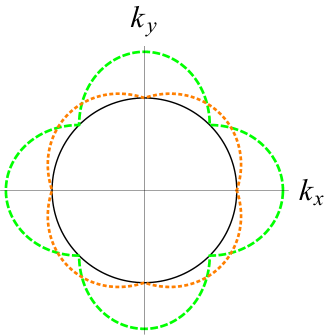
(a)  Competing order

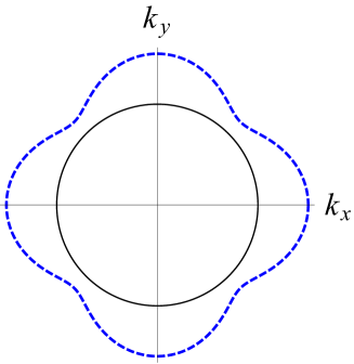
(b)  Full gap

Figure 1: (a) The black circle representing the Fermi surface is shown together with the angular dependent gap amplitudes. The dashed green curve is the $d$-wave gap $\Delta_{0}$, and the smaller dotted orange curve is the induced $d^{\prime}$-wave gap $\Delta_{1}$. For display purposes, the relative proportion of the gaps has not been preserved in the plot.  (b) Outside the black circular Fermi surface, the total gap $\sqrt{|\Delta_{0}|^{2}+|\Delta_{1}|^{2}}$ of the fully gapped $d+id^{\prime}$ state is shown in blue. The former gapless node lines of the $d$-state, which are the diagonals w.r.t. the $[100]$ and $[010]$ crystallographic directions, are sealed by the induced imaginary component $id^{\prime}$, which renders the overall $d+id^{\prime}$ state fully gapped.

To a good approximation, the angular momentum $L_{z}$ of the whole sample about $z$ is related to $\Delta_{0},\Delta_{1}$ (see Appendix A for derivation) by:

$$|\Delta_{1}|=|\Delta_{0}|\frac{|\langle L_{z}\rangle|}{\,2\hbar\;g\;(V/a^{2}c)}\;.$$ (4)

Here the components of the order parameter have been assumed to be spatially uniform within the sample, which is justified to a good approximation for sample sizes much smaller than the characteristic length of variation of the SC wave function; $(a^{2}c)$ denotes the unit cell volume of the SC’s crystal structure (being $c$ the edge $\parallel\hat{z}\parallel B$ field, $a\approx 4$Å, $c\approx 10$Å), $V$ the volume of the SC sample, and $g\sim 0.1$ the superconducting fraction of the material.

COULOMB BLOCKADE	ANGULAR MOMENTUM BLOCKADE
Charge $Q$ = deposit of electric potential energy	Angular momentum $L$ = deposit of mechanical energy
Electrostatic potential $V_{\text{max}}$: beyond which there is spontaneous discharge	Angular velocity $\omega_{\text{max}}$: beyond which the centrifugal stress results in breaking
Discharge: decreasing $V$	Discharge: decreasing $\omega$
Capacitance $C\,\propto$ area of the plates	Moment of intertia $I_{\text{in}}$ : increasing with spreading of the mass distribution about the rotation axis
$Q=C\;V$	$L=I_{\text{in}}\;\omega$
Energy $E=CV^{2}/2$	Energy $E=I_{\text{in}}\;\omega^{2}/2$
Current $i$	Torque $\tau$

Table 1: Mapping of the fundamental quantities and relations relevant to the Coulomb blockade to their corresponding quantities for the angular momentum blockade.

Let us define the non-negative integer variable $l\equiv|\langle L_{z}\rangle|/(2\hbar)$ and the characteristic area $S_{0}\equiv a^{2}c/(d\cdot g)$, where $d$ is the sample thickness and $V=Ad$ is the volume. This gives

$$|\Delta_{1}|=l\;|\Delta_{0}|\frac{S_{0}}{A}\;.$$ (5)

In the case of an isotropic gradient tensor $K_{ij}$, and if the grain is small enough to allow us neglect the spatial dependence of $\Delta_{0}(\vec{r}),\Delta_{1}(\vec{r})$, the GL functional takes the form

$$F=\int_{V=Ad}{d^{3}r\;\left[\alpha\,|\Delta_{0}|^{2}+\frac{\beta_{0}}{4}|\Delta_{0}|^{4}+K\left|(-i\frac{e}{c}\vec{A})\Delta_{0}\right|^{2}-\eta B|\Delta_{0}||\Delta_{1}|+\frac{N_{0}}{2}|\Delta_{1}|^{2}\right]}\;,$$ (6)

provided that we omit the magnetic field self-energy term, which does not affect the behavior of the magnetization or the susceptibility that we are going to describe. In the Coulomb gauge $\vec{A}(\vec{r})=\frac{B}{2}(-y,x)$, Eq. (5) gives

$$F(B,\langle L_{z}\rangle)=\int_{V=Ad}{d^{3}r\;\left[\alpha\,|\Delta_{0}|^{2}+\frac{\beta_{0}}{4}|\Delta_{0}|^{4}+K\frac{e^{2}}{c^{2}}\frac{B^{2}}{4}r^{2}\left|\Delta_{0}\right|^{2}-\eta B\;|\Delta_{0}|^{2}\frac{S_{0}}{A}\,l+\frac{N_{0}}{2}|\Delta_{0}|^{2}\frac{S_{0}^{2}}{A^{2}}\,l^{2}\right]}\;.$$ (7)

The coupling constant $\eta$ is derived and discussed in the Appendix of Ref. Balatsky2000 .

In the same way as the Coulomb blockade leads to jumps in charges and in charging energy, the analogous phenomena for the angular momentum blockade involve changes in angular momentum and magnetization. There will be jumps and spikes in magnetization and susceptibility, respectively, which we will now consider. The free energy $F$ is minimized by an optimal integer value of $l$ for each value of the applied field $B$. Hence $l$ forms a stepwise function of $B$ with steps at the switching fields $B=B_{l}$. The derivative $\partial l/\partial B$ is a sequence of delta function spikes at the switching fields that should be experimentally measurable. We will now consider these phenomena in detail.

The free energy density can be rewritten as

$$F_{v}(|\langle L_{z}\rangle|=2\hbar l,B)\equiv\frac{F(|\langle L_{z}\rangle|=2\hbar l,B)}{V}=const+aB^{2}-bBl+cl^{2}\;,$$ (8)

forming a piecewise parabolic function, where the following constants were introduced for convenience: $a\equiv K\frac{e^{2}}{c^{2}}\frac{A|\Delta_{0}|^{2}}{8\pi},b\equiv\eta|\Delta_{0}|^{2}\frac{S_{0}}{A},c\equiv\frac{N_{0}}{2}|\Delta_{0}|^{2}\frac{S_{0}^{2}}{A^{2}}$. The critical values $B_{n}$ where the optimal $l$ switches from $l=n$ to $l=n+1$ are obtained from the level crossings of the functions $F(l=n,B)$ and $F(l=n+1,B)$, which gives

$$B_{n}=\frac{c}{b}(2n+1)\;.$$ (9)

Hence the angular momentum value $\langle L_{z}\rangle=n\,(2\hbar)$ is attained for $B_{n-1}<B<B_{n}$. The integer $n$ will henceforth denote the integer that minimizes $F_{v}$, which is given by the integer part of $(1+(b/c)B)/2$. The magnetization and the susceptibility then become

$$M_{v}=-\frac{\partial F_{v}}{\partial B}=-2aB+bn\;,$$ (10)

and

$$\chi_{v}=\frac{\partial M_{v}}{\partial B}=-2a+b\sum_{n}\delta(B-B_{n})\;.$$ (11)

Except for the non-regular behavior at critical values (9) of the field, the magnetic susceptibility should have the constant value $\chi=-\frac{1}{4\pi}K\frac{e^{2}}{c^{2}}A|\Delta_{0}|^{2}$. The free energy density has cusps joining different parabolic arcs at each critical value for the magnetic field. The magnetization has constant jumps inversely proportional to $V$ (connecting regions of linear behavior). Finally, the susceptibility has $\delta$-like spikes inversely proportional to $V$.

III Behavior of magnetic observables

Let $x\equiv\frac{A}{S_{0}}$ be the dimensionless area and $y\equiv\frac{b}{c}B$ the dimensionless magnetic field. In terms of these quantities we have $a=\frac{1}{8\pi}K\frac{e^{2}}{c^{2}}S_{0}|\Delta_{0}|^{2}x,b=\eta|\Delta_{0}|^{2}\frac{1}{x},c=\frac{N_{0}}{2}|\Delta_{0}|^{2}\frac{1}{x^{2}},B=\frac{c}{b}y=\frac{N_{0}}{2\eta}\frac{y}{x}\approx\frac{E_{\rm F}}{2\mu_{\rm B}}\frac{y}{x}\;\,.$ Then the free energy density, magnetization, and susceptibility are given by

$$F_{v}=const+\frac{1}{8\pi}K\frac{e^{2}}{c^{2}}S_{0}|\Delta_{0}|^{2}\left(\frac{E_{\rm F}}{2\mu_{\rm B}}\right)^{2}\frac{y^{2}}{x}-\frac{N_{0}|\Delta_{0}|^{2}}{2}\frac{yn-n^{2}}{x^{2}}\;,$$ (12)

$$M_{v}=-\frac{1}{8\pi}K\frac{e^{2}}{c^{2}}S_{0}|\Delta_{0}|^{2}\frac{E_{\rm F}}{\mu_{\rm B}}\;y+\frac{N_{0}|\Delta_{0}|^{2}\mu_{\rm B}}{E_{\rm F}}\frac{n}{x}\;,$$ (13)

$$\chi_{v}=-\frac{1}{4\pi}K\frac{e^{2}}{c^{2}}S_{0}|\Delta_{0}|^{2}x+\frac{2\eta^{2}|\Delta_{0}|^{2}}{N_{0}}\sum_{n}\delta(y-(2n+1))\;.$$ (14)

The magnetization (13) in terms of the original dimensionful parameters takes the form

$$\quad M_{v}(B)=-\frac{1}{8\pi}K\frac{e^{2}}{c^{2}}\frac{(a^{2}c)}{g\cdot d}|\Delta_{0}|^{2}\frac{E_{\rm F}}{\mu_{\rm B}}\;y+\frac{N_{0}|\Delta_{0}|^{2}\mu_{\rm B}}{E_{\rm F}}\frac{a^{2}c}{gAd}n\;.$$ (15)

The second term is responsible for jumps of $M_{v}$ at each critical value of the magnetic field. All these jumps have the same amplitude and mutual spacing. The first term is due to the minimal coupling between the magnetic gauge potential and the order parameter. This contains the gradient tensor, and leads to a smooth monotonic variation of the magnetization between consecutive jumps.

The magnitude of the magnetization jumps $\Delta M_{\rm blockade}$ associated to the blockade mechanism increases if the sample area $A$ decreases. In fact, the jump size grows as $A^{-1}$ although remaining subleading with respect to the continuous variation $\Delta M_{\text{cont}}$ between jumps, even for tiny areas $A$. The first term in Eq. (15) is unaffected by $A$.

The ratio between the two contributions to $M_{v}(B)$ is

$$\frac{\left|\Delta M_{\rm blockade}\right|}{\left|\Delta M_{\rm cont}\right|}=\frac{A_{\rm cr}}{A}\;,$$ (16)

where $A_{\rm cr}\equiv\frac{4\pi N_{0}}{K}\left(\frac{c\,\mu_{\rm B}}{eE_{\rm F}}\right)^{2}\sim 1.20\;\text{\AA}^{2}$ is a critical area independent of any macroscopic feature of the SC sample. The magnetization and susceptibility given by Eqs. (13)-(14) are plotted in Figs. 2-4. In the plots a cylindrical sample is assumed with dimensions $V=d\cdot A\equiv 100\text{ \AA}\times(100\text{ nm})^{2}$. The blockade contribution alone to the magnetization is depicted in Fig. 3. The dimensionless term $K\frac{e^{2}}{c^{2}}S_{0}|\Delta_{0}|^{2}x$ is proportional to the area $A$, this is the only parameter on which it depends (among the parameters thickness $d$, area $A$ and magnetic field $B$), and its value affects the plot of the volume susceptibility in Fig. 4.

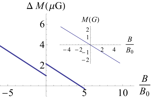
Figure 2: Magnetization $\Delta M$ of the sample (up to an additive constant), plotted in microgauss for the example case of area $A=(100\text{ nm})^{2}$ and thickness $d=100\text{ \AA}$, as a function of the magnetic field $B/B_{0}$, where $B_{0}\equiv N_{0}(a^{2}c)/(2\,\eta\,g\,A\,d)\sim 0.7\text{ tesla}$ for such a grain volume. In this plot, the field variable $B/B_{0}$ is centered about a critical level crossing point (i.e. any odd integer) and then zoomed by a $10^{6}$ factor. It is evident how this sample volume entails magnetization jumps $\sim 1\mu\text{G}$ . The background gradient tensor contribution to the magnetization is by far the leading one, being the jumps comparatively micro-scopic (see formula (16)): it is represented in units of gauss (with no scaling for the axis) in the inset at the top right, for a sample of thickness $d=100\text{ \AA}$ .

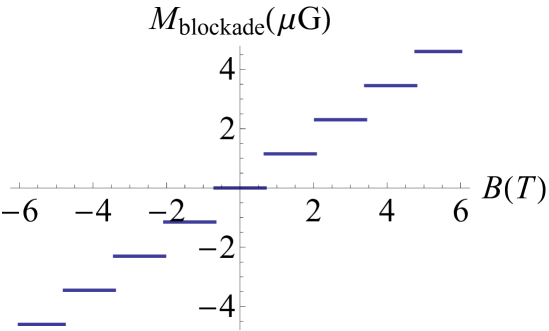
Figure 3: Blockade contribution to the magnetization of the sample, as a function of the magnetic field $B$ expressed in tesla, for a cylindrical grain of thickness $d=100$ Å and area $A=(100\text{ nm})^{2}$. The system displays a staircase of magnetization jumps of the order of $\sim 1\mu$ G, which are mutually spaced by regular intervals $\Delta B\sim 1.4$ T.

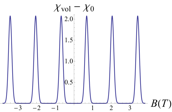
Figure 4: (Dimensionless) volume susceptibility of the sample, plotted againts the magnetic field $B$ for a cylindrical sample of thickness $d=100\text{\AA}$ and area $A=(100\text{ nm})^{2}$; the vertical axis is in units of $10^{-9}$. There is a background smooth contribution $\chi_{0}$ to the susceptibility (about $-3\cdot 10^{-4}$ for this grain) due to the gradient term of the GL functional, which is proportional to the area $A$ of the sample, and $\delta$-like spikes above it, due to the angular momentum blockade, which are $\propto\,V^{-1}$, and mutually spaced by regular intervals $\Delta B\sim$ 1.4 T .

IV Conclusions

In conclusion we propose the notion of angular momentum blockade in granular $d$-wave superconductors. The effect is due to abrupt changes in the angular momentum of the electron liquid in the condensate. The pure $d$-wave state has $L_{z}=0$. As an out-of-plane magnetic field is applied to the sample, a chiral $d^{\prime}$-component is induced. The angular momentum of Cooper pairs has to vary accordingly. This process of conversion of momentum, from $L_{z}=0$ to a finite value given by the induced $d^{\prime}$ component, proceeds in a series of steps where individual Cooper pairs acquire finite angular momentum. These steps are what we call angular momentum blockade. Jumps in the angular momentum of the condensate result in jumps of the magnetization, which we calculate. We find that these steps occur at well-defined values of magnetic field. We also have defined a ”characteristic area” $S_{0}$ ($\propto$ inverse thickness $d^{-1}$), providing a scale for the change of induced gaps $|\Delta_{1}|$ between two critical fields causing steps in magnetization, in units of the $d$-wave gap amplitude $|\Delta_{0}|$. On the other hand, we have provided a ”critical area” $A_{\text{cr}}$, which is the area scale related to the relevant weight between the two distinct contributions entering the magnetization variation (within the same magnetic field range considered above): the blockade contribution w.r.t. the gradient tensor one.
As illustrated in Figs. 2,3, a nanoscale grain of typical volume $10^{5}\,\text{nm}^{3}$ should exhibit significant magnetization jumps of the order of 1 microgauss, which are encountered at critical magnetic fields whose uniform mutual spacings we estimate being of the order of $\sim$ 1 tesla. These results suggest that sensitive magnetization experiments might be able to see these jumps. Finally in Fig. 4 two different contributions to the magnetic susceptibility are highlighted: the gradient term contribution, which is a constant background value proportional to the area $A$ of the sample, and the angular momentum blockade contribution, consisting of $\delta$-like spikes $\propto\,V^{-1}$, and mutually spaced by regular intervals $\Delta B$ ($\sim$ 1 tesla for the example grain).

Acknowledgements This work has been supported by the Swedish Research Council grants VR 621-2012-298, VR 621-2012-3984, ERC and DOE. We are grateful to B. Altshuler for an earlier discussion of angular momentum blockade.

Appendix A Relation between the angular momentum and the gaps for the $d$ and the $d^{\prime}$ components

We refer to the components of the SC wave function, having $d_{x^{2}-y^{2}}$ and $d_{xy}$ symmetry respectively, as $\psi_{0}$ and $\psi_{1}$. The angular momentum becomes

$$\langle L_{z}\rangle=\langle\psi_{0}(\theta)+\psi_{1}(\theta)|-i\hbar\partial_{\theta}|\psi_{0}(\theta)+\psi_{1}(\theta)\rangle=$$

$$=-i\hbar\int{dV\,\frac{d\theta}{2\pi}2[\psi_{0}^{*}\psi_{1}\cos(2\theta)^{2}-\psi_{0}\psi_{1}^{*}\sin(2\theta)^{2}]}=-i\hbar\int\,dV\;[\psi_{0}^{*}\psi_{1}-\psi_{0}\psi_{1}^{*}]\;.$$ (17)

In terms of respective moduli and phases $\psi_{0}=|\psi_{0}|\exp(i\nu_{0})$, $\psi_{1}=|\psi_{1}|\exp(i\nu_{1})$, the above equation becomes

$$\langle L_{z}\rangle=\int dV{[-\hbar 2|\psi_{0}||\psi_{1}|\sin(\nu_{0}-\nu_{1})]}\;.$$ (18)

Because of the global U(1) symmetry we can arbitrarily choose $\nu_{0}=0$ for this discussion, and the free energy is minimized when the relative phase $(\nu_{0}-\nu_{1})=\pm\pi/2$. For a spatially uniform wave function, i.e., a spatially uniform order parameter, it is

$$\langle L_{z}\rangle=V{[-\hbar 2|\psi_{0}||\psi_{1}|\sin(\nu_{0}-\nu_{1})]}\;.$$ (19)

For the minimizing relative phase $\pm\pi/2$ this gives

$$\langle L_{z}\rangle=V\left[{-\hbar 2|\psi_{0}|^{2}\frac{|\Delta_{1}|}{|\Delta_{0}|}}\right]\;,$$ (20)

since $|\Delta_{1}|/|\Delta_{0}|=|\psi_{1}|/|\psi_{0}|$. With $a^{2}c$ the unit cell volume, $d$ the sample thickness, and $V=Ad$ the sample volume, the number of Cooper pairs $N_{\text{sc}}$ in the grain is approximately

$$V|\psi_{0}|^{2}=N_{\text{sc}}=g\,\frac{V}{a^{2}c}\;,$$ (21)

where $g\sim 0.1$ is the high-$T_{c}$ superconducting fraction. This gives the estimate

$$|\Delta_{1}|=|\Delta_{0}|\frac{|\langle L_{z}\rangle|}{2\hbar gV/(a^{2}c)}\;.$$ (22)

Appendix B Numerical values

For allowing better checks, numerical values listed below come with more digits than the significative ones.

$$\begin{array}[]{lr}\text{Edges of the SC unit cell}&a\sim 4\text{\AA},\;c\sim 10\text{\AA}\\ \text{Coherence length}&\xi\sim 10\text{\AA}=10^{-7}\text{cm}\\ \text{Superconducting fraction}&g\sim 10^{-1}\\ \text{Unperturbed }d_{x^{2}-y^{2}}\text{-wave gap}&|\Delta_{0}|\sim 50\text{ meV}=8.011\times 10^{-14}\text{ erg}\\ \text{Density of states}&N_{0}\sim 2.4\times 10^{33}\text{ erg}^{-1}\text{ cm}^{-3}\\ \text{Fermi energy }&E_{F}\sim 1.98\times 10^{-12}\text{ erg}\\ \text{Thickness }&d\equiv 100\text{ \AA}=10^{-6}\text{cm}\\ \text{"Characteristic area"}&S_{0}\equiv\frac{(a^{2}c)}{d\cdot g}\sim 1.6\times 10^{-15}\text{cm}^{2}=16\text{ \AA}^{2}\\ \text{Modulus of the gradient tensor}&K\sim\hbar^{-2}\xi^{2}N_{0}\sim 2.156\times 10^{73}\text{ cm}^{-1}\text{s}^{-2}\text{erg}^{-3}\\ \text{Dimensionless recurrent combination}&K\frac{e^{2}}{c^{2}}S_{0}|\Delta_{0}|^{2}\sim 5.68\times 10^{-8}\\ \text{"Critical area"}&A_{\text{cr}}\sim 1.20\times 10^{-16}\text{cm}^{2}=1.20\;\text{\AA}^{2}\\ \end{array}$$

References

- (1) J. G. Bednorz and K. A. Müller, Zeitschrift für Physik B 64, 189 (1986)
- (2) D. A. Wollman, D. J. Van Harlingen, W. C. Lee, D. M. Ginsberg, and A. J. Leggett, Phys. Rev. Lett. 71, 2134 (1993)
- (3) W. N. Hardy, D. A. Bonn, D. C. Morgan, Ruixing Liang, and Kuan Zhang, Phys. Rev. Lett. 70, 3999 (1993)
- (4) Z. X. Shen, D. S. Dessau, B. O. Wells, D. M. King, W. E. Spicer, A. J. Arko, D. Marshall, L. W. Lombardo, A. Kapitulnik, P. Dickinson, S. Doniach, J. DiCarlo, A. G. Loeser, and C. H. Park, Phys. Rev. Lett. 70, 1553 (1993)
- (5) C. C. Tsuei and J. R. Kirtley, J. Phys. Chem. Solids 59, 2045 (1998)
- (6) T. Xiang and J. M. Wheatley, Phys. Rev. Lett. 76, 134 (1996)
- (7) K. A. Müller, Phil. Mag. Lett. 82, 279 (2002)
- (8) R. B. Laughlin, Phys. Rev. Lett. 80, 5188 (1998)
- (9) A. V. Balatsky, M. I. Salkola, and A. Rosengren, Phys. Rev. B 51, 15547 (1995)
- (10) R. Movshovich, M. A. Hubbard, M. B. Salamon, A. V. Balatsky, R. Yoshizaki, J. L. Sarrao, and M. Jaime, Phys. Rev. Lett. 80, 1968 (1998)
- (11) A. V. Balatsky, I. Vekhter, and Jian-Xin Zhu, Rev. Mod. Phys. 78, 373 (2006)
- (12) K. A. Müller, Nature 377, 133 (1995)
- (13) D. Gustafsson, D. Golubev, M. Fogelström, T. Claeson, S. Kubatkin, T. Bauch, and F. Lombardi, Nature Nanotech. 8, 25 (2013)
- (14) M. Fogelström, D. Rainer, and J. A. Sauls, Phys. Rev. Lett. 79, 281 (1997)
- (15) G. E. Volovik, JETP Lett. 66, 522 (1997)
- (16) A. V. Balatsky, Phys. Rev. B 61, 6940 (2000)
- (17) K. Krishana, N. P. Ong, Q. Li, G. D. Gu, and N. Koshizuka, Science 277, 83 (1997)
- (18) H. Aubin, K. Behnia, S. Ooi, and T. Tamegai, Phys. Rev. Lett. 82, 624 (1999)
- (19) G. Leibovitch, R. Beck, Y. Dagan, S. Hacohen, and G. Deutscher, Phys. Rev. B 77, 094522 (2008)
- (20) A. V. Balatsky and R. Movshovich, Physica B 259-261, 446 (1999); A.V. Balatsky and R. Movshovich, cond-mat/9805345 (unpublished).
- (21) L. Kouwenhoven and C. Marcus, Physics World 11, 35 (1998)
- (22) V. N. Gladilin, V. M. Fomin, and J. T. Devreese, Phys. Rev. B 70, 144506 (2004)
- (23) A. V. Balatsky, Phys. Rev. Lett. 80, 1972 (1998)