C IV Line-Width Anomalies: The Perils of Low $S/N$ Spectra

Abstract

Comparison of six high-redshift quasar spectra obtained with the Large Binocular Telescope with previous observations from the Sloan Digital Sky Survey shows that failure to correctly identify absorption and other problems with accurate characterization of the C iv $\lambda 1549$ emission line profile in low $S/N$ data can severely limit the reliability of single-epoch mass estimates based on the C iv emission line. We combine the analysis of these new high-quality data with a reanalysis of three other samples based on high $S/N$ spectra of the C iv emission line region. We find that a large scatter between the H$\beta$- and C iv-based masses remains even for this high $S/N$ sample when using the FWHM to characterize the BLR velocity dispersion and the standard virial assumption to calculate the mass. However, we demonstrate that using high-quality data and the line dispersion to characterize the C iv line width leads to a high level of consistency between C iv- and H$\beta$-based masses, with $<0.3$  dex of observed scatter, and an estimated $\sim$0.2  dex intrinsic scatter, in the mass residuals.

1. INTRODUCTION

In the well-accepted paradigm of galaxy formation and evolution from hierarchical structure growth, it is simple enough to reach the conclusion that all massive galaxies should house supermassive black holes (BHs; see also Sołtan 1982). Unfortunately, it is not as simple a task to measure BH masses, growth rates, and their evolution. BH mass measurements using dynamical methods in quiescent galaxies (see e.g., Gebhardt et al. 2003 and compilations such as Ferrarese & Ford 2005; Graham 2008; Gültekin et al. 2009) require high spatial resolution and are thus restricted to the local universe. On the other hand, reverberation mapping (RM; Blandford & McKee, 1982; Peterson, 1993) is a successful method for directly measuring BH masses in active galaxies. While not restricted by spatial resolution, reverberation mapping is dependent on temporal resolution. Thus, distance is not a fundamental restriction, but obtaining the long-term observing resources to meet the temporal sampling requirements has logistically driven most reverberation experiments to target lower-luminosity, faster varying AGNs in the local universe, $z\lesssim 0.3$. Nonetheless, scaling relationships derived from reverberation mapping results of the local AGN population (e.g. Vestergaard & Peterson, 2006; McGill et al., 2008; Rafiee & Hall, 2011b; Bentz et al., 2013) enable a means for studying BH masses in Type 1 (broad-line) AGNs at all redshifts based on single-epoch (SE) mass estimates (see, e.g., Vestergaard, 2004; Vestergaard & Osmer, 2009; Kelly et al., 2010; Shen et al., 2011).

These SE BH mass estimates depend on several assumptions. First, the luminosity of the AGN continuum, measured from the spectrum near a broad emission line of interest, must be a valid proxy for the broad line region radius (BLR). In theory, this is expected because photoionization physics regulates the production of line-emitting photons in such a way that the characteristic radius of emission, $R_{\rm BLR}$, scales tightly with the nuclear luminosity, $L$ (Davidson, 1972; Krolik & McKee, 1978). More importantly, direct reverberation mapping measurements of $R_{\rm BLR}$ show the expected correlation and provide an empirically well-calibrated $R_{\rm BLR}-L$ relation (Kaspi et al., 2000; Bentz et al., 2009a, 2013). The indirect BLR radius is then combined with a broad emission-line width from at least one broad emission line (H$\alpha$, H$\beta$, Mg ii $\lambda 2800$, or C iv $\lambda 1549$) with a calibrated scaling relation. This width is assumed to be representative of the BLR gas velocity under the influence of the gravity of the central black hole. Given these assumptions, the virial BH mass is estimated by $M_{\rm BH}=fR_{\rm BLR}(\Delta V)^{2}/G$, where $R_{\rm BLR}$ scales as $\sim L^{1/2}$, $\Delta V$ is the velocity dispersion of the BLR gas, $G$ is the gravitational constant, and $f$ is a dimensionless factor of order unity accounting for the unknown BLR geometry and kinematics and determined from local calibrations (cf. Onken et al., 2004; Woo et al., 2010; Park et al., 2012a; Grier et al., 2013a).

At redshifts $z\gtrsim 2$, all emission lines but C iv $\lambda 1549$ have redshifted out of the optical observing window, making it the only emission line available for high-$z$ BH and galaxy evolution studies using ground-based optical data. However, several past studies have claimed that C iv is an unreliable virial mass indicator (e.g., Baskin & Laor 2005; Sulentic et al. 2007; Netzer et al. 2007, hereafter N07; Shen & Liu 2012; Trakhtenbrot & Netzer 2012) due to large scatter and possible offsets in the C iv based masses compared to H$\alpha$, H$\beta$, or Mg ii. The most wide-spread, physically motivated argument against C iv is tied to the commonly observed blueward asymmetries, enhancements, and velocity shifts of the C iv line profile. It has been suggested that these observed properties are the result of non-virial motions of the C iv-emitting gas (i.e., outflows, winds, and non-gravitational forces; Gaskell, 1982; Wilkes, 1984; Richards et al., 2002; Leighly & Moore, 2004), rendering C iv velocity width measurements unsuitable for estimating BH masses. We should note, however, that as with stellar winds, any radiatively driven wind will result in a velocity comparable to the escape velocity (Cassinelli & Castor, 1973), which is close enough to the virial velocity that it is unlikely to be a considerable issue given the other uncertainties in the problem. Other studies have found general consistency between single-epoch C iv and H$\beta$ masses (e.g., Vestergaard & Peterson 2006, hereafter VP06; Greene et al. 2010; Assef et al. 2011, hereafter A11), suggesting that any biases are modest. The only way to definitively probe the C iv BLR kinematics and search for potential non-virial motions is using reverberation mapping experiments of the C iv emission. These experiments isolate the photoionized, and apparently virialized (Peterson & Wandel, 1999, 2000), gas in the BLR that is responding to the continuum variability from other non-variable emission components. Further constraints on the geometry and kinematics are then possible with two-dimensional velocity–delay maps (see, e.g., Horne et al., 2004; Bentz et al., 2010; Pancoast et al., 2012; Grier et al., 2013b), but unambiguous maps have yet to be constructed for this emission line (though see Ulrich & Horne, 1996). Nonetheless, available reverberation mapping results for C iv yield consistent results with those of the other emission lines observed in the same objects (Peterson & Wandel, 1999, 2000; Peterson et al., 2004), so any issues are restricted to SE estimates using C iv, rather than C iv in general.

One concern contributing to the C iv debate is that sample selection may be a problem. For example, VP06 studied only local reverberation-mapped AGNs. Richards et al. (2011) show that this sample does not span the full C iv equivalent width/blueshift parameter space observed for Sloan Digital Sky Survey (SDSS) quasars, suggesting that the results may not be representative of the overall high-redshift quasar population, and raise the concern that BH mass scaling relationships calibrated only with low blueshift sources may not be applicable to the large blueshift, low equivalent width (“wind-dominated”) sources. On the other hand, the VP06 reverberation mapping sample spans a rest-UV luminosity range of 3 orders of magnitude. This is much larger than most studies (e.g., N07; Dietrich et al. 2009, hereafter D09; Shen & Liu 2012; Ho et al. 2012), making it far easier to recognize the existence of an underlying correlation in the presence of noise. Indeed, the studies finding little or no correlation (e.g., D09; Greene et al. 2010; Shen & Liu 2012; Ho et al. 2012) first restrict the sample to such a narrow luminosity range that no correlation would be found for any estimator, including H$\beta$. A11 pointed out that roughly half of the ‘problem’ has nothing to do with the line widths but comes from the variance between the continuum estimates rather than the line structure. Denney (2012) then argued that much of the discrepancy due to the line widths between H$\beta$ and C iv-based SE BH mass estimates is due to a non-variable component of the C iv emission-line that biases the full width at half maximum (FWHM) line widths often used to derive the SE BH mass. Since the component biasing the FWHM seems not to reverberate, direct BH mass measurements based on reverberation mapping are unaffected, leading to the better agreement with results for H$\beta$.

C iv supporters also argue that data quality is a key factor: VP06 largely used high-$S/N$ HST spectra or an average reverberation mapping campaign spectrum, and A11 obtained new or previously published high-$S/N$ C iv spectra of all their targets. Most studies instead use C iv observations in lower $S/N$ survey spectra, such as from SDSS. VP06, A11, and Denney (2012) demonstrate (1) that the scatter in the C iv-to-H$\beta$ masses or line widths is reduced when low-$S/N$ spectral data are removed, and (2) that low $S/N$ can mask absorption in the C iv line profile, leading to some of the highly discrepant C iv-to-H$\beta$ masses of N07 and Baskin & Laor (2005). Even without these complicating issues, the uncertainty in the velocity field of the BLR gas, as derived from a SE line-width characterization, is already the largest source of systematic uncertainty in SE mass estimates due to the unknown geometry, kinematics, and inclination of the BLR (Woo et al., 2010). When width measurements are routinely made from survey data of varying quality, these uncertainties are enhanced. These fractional velocity errors are magnified in the mass estimates that depend on $\Delta V^{2}$.

SE BH mass measurements are used to draw conclusions about black hole demographics, growth rates, BLR gas kinematics, accretion and feedback physics, and the evolution of all these properties across cosmic time (Vestergaard & Osmer, 2009; Kelly et al., 2010; Conroy & White, 2013; Shankar et al., 2013; Trump et al., 2013). A clear understanding of the effects that data quality and analysis practices have on the accuracy and precision of these line width measurements and BH mass estimates is therefore crucial. In this work, we attempt to reconcile the evidence and arguments on both sides of this debate as to the reliability of BH mass estimates based on C iv in the context of data quality. We first select one of the studies that (1) conclude that C iv is a poor virial mass estimator based on a large scatter between C iv- and H$\beta$-based black hole masses (albeit over a very limited dynamic range in luminosity), and (2) base their conclusion solely on survey-quality (i.e., typically low $S/N$) data of the C iv line. For this, we select the work of N07, who present a sample of 15 high-$z$ quasars with C iv masses based on spectra from SDSS and H$\beta$ masses determined using Gemini Near-Infrared Spectrograph observations. By obtaining new, high-$S/N$ spectra of a portion of this sample and combining it with other high-quality data from the literature, we investigate whether data quality can explain the discrepancy between C iv- and H$\beta$-based BH mass estimates. We define high-quality spectra as those with $S/N\geq$10 pixel^-1 measured in an emission-line-free region of the continuum ($\sim$1450Å or $\sim$1700Å in the rest frame).

In Section 2, we present spectra of six high-redshift quasars from the N07 sample observed with the first of the Multi-Object Double Spectrographs (MODS1; Pogge et al., 2010) on the Large Binocular Telescope (LBT) and give details of the additional samples we select from the literature and public archives to increase our total sample size to 47 AGNs. In Section 3 we describe how we fit the C iv line profiles, and Section 4 describes our line width, luminosity, and BH mass measurements. We then compare the C iv and H$\beta$ masses derived from our high-quality sample in Section 5. In Section 6 we discuss the impact data quality has on (1) the presence of absorption in the C iv profile, (2) the C iv line width measurements, and (3) the SE C iv BH masses in relation to H$\beta$ masses. A summary and concluding remarks are given in Section 7.

2. Sample Selection and Observations

2.1. N07 Sample

Figure 1.— Restframe UV spectra of the six high-redshift quasars observed with MODS1 on LBT. These are all SDSS targets from N07. The arrows indicate the location of atmospheric O₂ A-band and B-band absorption observed at observed wavelengths 7620Å and 6880Å, respectively.

We used the MODS1 spectrograph on the LBT to obtain rest-frame UV spectra of six of the 15 high-redshift quasars presented by N07 (Table 1; we will refer to targets by the leading digits in their names, e.g., J0254 for SDSS J025438.37+002132.8). These six quasars were chosen from the full N07 sample because of their favorable location on the sky during our observing runs rather than their particular spectral properties or C iv versus H$\beta$ mass estimates.

For each quasar we used either the red or blue channel of MODS1 without the dichroic, depending on the observed wavelength of the redshifted C IV $\lambda$1549 emission line. The blue-channel spectra used the G400L grating (400 lines mm^-1 in first order), and the red-channel spectra used the G670L grating (250 lines mm^-1 in first order) with a GG495 order blocking filter. For all spectra we used the 0$\farcs$6 segmented long-slit mask (LS5x60x0.6), centering the quasar in the slit. This slit width gives a nominal resolution of $\lambda/\Delta\lambda\approx$2000, with wavelength coverage from 3200$-$6000Å in the blue channel and 6000$-$10000Å in the red channel. All of the quasars were observed near meridian crossing so we did not need to orient the slit along the parallactic angle to minimize the effects of differential atmospheric refraction (MODS does not have an atmospheric dispersion corrector). Multiple exposures (3 or 4) were used to control for cosmic rays. The observations and observing conditions are summarized in Table 1.

After processing the images using MODS-specific two-dimensional calibration procedures (bias and flat field), the spectra were extracted and then wavelength and flux calibrated using standard procedures in the IRAF twodspec and onedspec packages. The spectral resolution of the MODS1-Blue (-Red) channel targets is roughly 2.2Å (3.5Å) near the C IV emission line. We resampled the spectra of J0254, J1055, J1159, and J1537 onto a linear wavelengths scale with 0.5Å pixel^-1, and J2102 and J2103 onto a linear wavelength scale with 0.75Å pixel^-1. Figure 1 shows the MODS1 spectra of our six targets.

Although spectrophotometric standard stars were observed as part of the overall queue observing programs for the nights, the variable observing conditions resulted in an unreliable absolute flux calibration. Thus, the spectra in Figure 1 are in uncalibrated $F_{\lambda}$ units. Unfortunately, telluric standards were also not observed. Telluric absorption is present to some degree in the C iv profiles of all targets except J0254; however, it is typically only present in the line wing and does not hinder our ability to model the line profile or measure the line width. The exceptions to this are for J1159 and J1537. In the case of J1159, we did not include corrections because of the proximity of the absorption to the profile peak plus the additional intrinsic (or intervening) absorption. For J1537, the spectrophotometric standard taken the same night differed in airmass by only $\sec(z)\sim 0.1$. We therefore performed a crude correction for the O₂ A-band and B-band by dividing the standard star spectrum with templates derived from the HST CALSPEC database and then using the NOAO onedspec package TELLURIC task to scale the telluric correction. Some residual absorption at the optically thick, and therefore nonlinear, core of the O₂ band head remains due to the imperfect match in seeing and/or airmass, but we later masked any remaining telluric absorption when we fit the C iv profiles (see Section 3).

In order to make a meaningful comparison with the original SDSS spectra, we performed a homogeneous analysis of both the original SDSS spectra and the MODS1 spectra of these six quasars. The SDSS spectra were rebinned to a linear wavelength dispersion consistent with the pixel size at restframe $\lambda$1549Å in each SDSS spectrum. This resulted in dispersions of 1.2Å pixel^-1 for J0254, and 1.5Å pixel^-1 for J1055, J1159, J1537, J2102, and J2103. The spectral resolution in this region was calculated to be 2.2–2.3Å for all sources.

2.2. Additional Literature Samples

We expand our sample of high $S/N$ spectra by including three additional samples. First, we use eight objects from A11, excluding the broad-absorption line quasar H1413+117 and objects classified as having Group II, poorer quality, line widths (see A11 Table 3 and Section 3). Second, we include six of the 10 objects presented by D09 that fit our quality requirement of $S/N>10$  pix^-1 and do not have a broad absorption-line region obscuring the blue side of the C iv profile. Third, we fully reanalyze all the high $S/N$ UV spectra of the reverberation mapping sample (e.g., Peterson et al., 2004; Bentz et al., 2008; Denney et al., 2010; Grier et al., 2012) in the MAST archives. Much of this sample overlaps with that presented by VP06, but we have updated it with recent high-resolution spectra taken with either the HST Cosmic Origins Spectrograph (COS) or Space Telescope Imaging Spectrograph (STIS). In a limited number of cases, we averaged multiple epochs that were closely spaced in time to increase the $S/N$, but we otherwise dropped spectra/targets that did not meet our $S/N$ requirement, leaving 27 objects in the RM sample. Our full sample therefore contains 47 objects. Figure 2 shows the redshift and UV luminosity distributions and the relation between C iv blueshift and equivalent width (discussed by Richards et al., 2011) for our sample. The former two distributions (left and center panels of Figure 2) demonstrate that our sample, though not large by survey standards, spans redshifts 0$\;\stackrel{{\scriptstyle<}}{{\sim}}\;$ $z$$\;\stackrel{{\scriptstyle<}}{{\sim}}\;$ 3.5 and five orders of magnitude in AGN luminosity. The right panel shows that while this sample spans a broad range of C iv equivalent widths (EQW), there is, unfortunately, still only one object — Q2302 from the D09 sample — that has a low C iv EQW and a large blueshift. It is, however, an extreme example of this phenomenon.

Figure 2.— Properties of our complete sample. The left panel shows the distribution of redshifts, the middle panel shows the UV continuum luminosity distribution, and the right panel shows the location of our sample in the C iv blueshift–equivalent width parameter space described by Richards et al. (2011).

3. C IV Line Profile Fits

There is no universally accepted method for separating the various blended components of emission in AGN spectra or for setting line boundaries for measuring emission-line widths (see, e.g., A11; Vestergaard et al., 2011; Park et al., 2012b; Shen & Liu, 2012). Denney et al. (2009a) also demonstrate that fitting functional forms to the H$\beta$ profile can exacerbate, rather than mitigate, systematic problems in the H$\beta$ line width measurements. In general, this is true only of low $S/N$ data, and is therefore not a concern here. Regardless of data quality, reliably measuring the C iv line widths without a model for the intrinsic line shape is impossible in the presence of absorption in the line profile and blending with the “red shelf” emission often seen between C iv and He ii (see Fine et al., 2010; Assef et al., 2011, and references therein). Using functional fits is therefore a common practice under these circumstances, and thus, utilized here.

We chose a simple approach for fitting the C iv emission region that closely follows the “Prescription A” approach described by A11 and the continuum fitting of Fine et al. (2010) methods (1) and (2). We fit and subtract a linear local continuum, fitting to a region blueward of C iv (rest wavelength $\sim$1450Å, or $\sim$1350Å in a few cases where the $\sim$1450Å region is contaminated by absorption) and redward of He ii  $\lambda$1640 and O iii]  $\lambda$1663 (at $\sim$1700Å). By selecting the continuum windows this way, the red shelf lies within our fitting window. We do not assume an origin for this emission for our fits. Instead, we set our redward C iv line boundary well into the red shelf and mask out the wavelength region covered by the red shelf during the fit. We select this region independently for each object, but typically start the mask between $\sim$1580$-$1600Å and extend it to the red edge of O iii], $\sim$1690Å. We also mask out any absorption regions and N iv] $\lambda$1486 emission, when it is observed.

We then fit the unmasked regions of the continuum-subtracted C iv line profiles with sixth-order Gauss-Hermite (GH) polynomials using the normalization of van der Marel & Franx (1993) and the functional forms of Cappellari et al. (2002). The best-fitting coefficients are determined with a Levenberg-Marquardt least-squares fitting procedure. Constraints from the unmasked line and continuum regions provide interpolation through the masked regions. This approach minimizes the number of components that are fit to the spectra, minimizing problems that can be introduced by the use of multiple model fits to blended emission components (e.g., Denney et al., 2009a).

We do not constrain the number of GH fit components required to reproduce the observed C iv profile, although typically, only two components are required. We do not attribute individual fit components to kinematically distinct regions (e.g., narrow-line region (NLR) as compared to BLR components). Some studies (Baskin & Laor, 2005; Sulentic et al., 2007; Greene et al., 2010; Shen & Liu, 2012) remove a narrow-line component, under the assumption that this emission arises in a low-density, extended kiloparsec-scale NLR. Based on the arguments by Denney (2012), including a demonstration that the non-reverberating, low-velocity component of the C iv line is much broader than the O iii$\lambda$5007 narrow emission line, we do not do so, and we use the full composite fit for our C iv line width measurements.

3.1. N07 Sample

Using these procedures, we fit both the MODS1 and SDSS spectra of the N07 sample. Our goal in refitting the latter is (1) to attempt to reproduce the line widths quoted by N07 based on these spectra, and (2) to make a meaningful comparison between these survey quality spectra and the high quality MODS1 spectra using the same modeling procedures. While profile fits can introduce systematics into the measured C iv widths of the low $S/N$ SDSS spectra, direct measurements of either the FWHM or line dispersion at these low signal-to-noise ratios are more systematically uncertain than those made using parametric fits (Denney et al., 2009a).

Exceptions to this standard fitting procedure were required for the MODS1 spectrum of J1159 and the SDSS spectrum of J0254. The MODS1 spectrum of J1159 (Figure 3a) shows significant absorption across the peak (both intrinsic and atmospheric), that prevents convergence to a physically-plausible GH-fit model. Instead, we used multiple Lorentzian profiles to fit the wings of the line profile, constraining the peak amplitude and wavelength by the slope of the line wings and the functional form of the Lorentzian profile. For the SDSS spectrum of J0254, we also did not achieve an acceptable GH polynomial fit, likely due to a combination of low $S/N$, the apparent absorption, and asymmetry in this profile. We obtained a somewhat more representative profile with two Gaussian components, in which the broader component is blueshifted relative to the narrower component.

The solid black curves in Figures 3a and 3b show the final models (black) for each spectrum (gray). For comparison, the horizontal black bar above the C iv profile in the top (SDSS) panels of Figures 3a and 3b represent the FWHM values given by N07. These bars are centered at the half maximum flux level and the theoretical C iv line center. N07 do not provide a description of how the line widths were measured or their uncertainties, so a direct comparison is not possible.

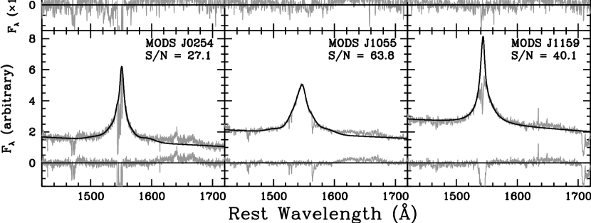
Figure 3a.— Spectra (gray), model fits (solid black), and residuals for the N07 sample objects J0254, J1055, and J1159 observed with SDSS (top) and MODS1 (bottom). The $S/N$ of each spectrum measured per resolution element in the continuum is given in the top corner of each panel. The black bar across the SDSS C iv profile (top) shows the FWHM velocity width reported for the C iv emission line in this object by N07.

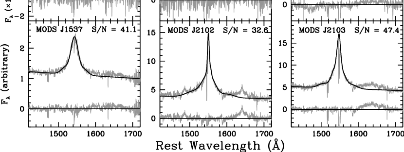
Figure 3b.— Same as Figure 3a but for the N07 sample objects J1537, J2102, and J2103.

3.2. Additional Samples from the Literature

We fit the spectra for the other samples in the same standard manner given above. Our fits to the D09 and RM C iv spectra are shown in Figures 4 and 5, respectively. More than one high quality spectrum is available for many of the objects in the RM sample, and in these cases we show a representative example. The C iv profile fits and exceptions to our standard fitting method for the A11 sample can be found in that work. The exceptions for the D09 and RM samples are:

[HB89] 0150-202: There is an unexplained, yet sharp, difference in the continuum slope on either side of the dichroic, just redward of the C iv line. A linear continuum fit was therefore not reliable, so we fit a local power-law continuum, based on regions $\sim$1350Å, $\sim$1450Å, and $\sim$1700Å.

PG0804: The HST/COS spectrum did not cover the $\sim$1700Å continuum window. We instead fit a linear continuum between $\sim$1320Å and $\sim$1450Å and extrapolated it to the red end of the available data.

PG1613: The HST/COS spectrum did not cover the $\sim$1700Å continuum window. However, there was also an IUE/SWP spectrum of this object. We used the IUE spectrum as a template for the $\sim$1700Å continuum window of the COS spectrum by scaling the IUE spectrum to match the $\sim$1450Å continuum flux of the COS spectrum. We extrapolated the flux redward of the COS spectrum using a constant value based on the last available pixel in the original spectrum. This region was masked out during the C iv profile fit. We further extrapolated the COS spectrum to create a template $\sim$1700Å continuum window using the scaled IUE spectrum flux values in this region. Figure 5 shows both the extrapolated COS spectrum (dark gray), scaled IUE spectrum (light gray), and the resulting GH polynomial fit. This extrapolation produces a more symmetric and realistic C iv profile than extrapolating a linear continuum fit between $\sim$1350Å and $\sim$1450Å, which resulted in a much steeper slope redward of C iv than expected based on comparison with the IUE spectrum.

Figure 4.— Spectra (gray), composite continuum plus C iv profile fits (solid black), and residuals for the D09 sample.

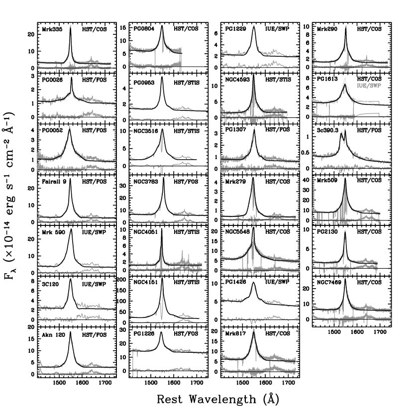
Figure 5.— Same as Figure 4 but for the RM sample.

4. Line Width, Luminosity, and BH Mass Determinations

4.1. H$\beta$

H$\beta$ line widths, optical luminosities or RM lag, and H$\beta$ masses were collected or recalculated from the literature as follows:

N07 sample: We use the H$\beta$ FWHM and 5100Å monochromatic AGN luminosity given by N07 to recalculate the H$\beta$-based masses directly from the calibration of the BLR $R-L$ relationship (Bentz et al. 2009a; Equation 4 of A11). N07 does not provide uncertainties in their measured quantities, so we have included a ‘typical’ uncertainty for the N07 H$\beta$ masses of 0.2 dex, based on the typical uncertainties in the H$\beta$ masses from the other samples we consider. Values are listed in Table 2.

A11 sample: We adopt the H$\beta$ masses for this sample directly from Table 5 of A11, but we recalculate the uncertainties from the line width and luminosity uncertainties given by A11 and the mass scaling relation zero-point uncertainty of $\sigma_{\log\langle f\rangle}=0.09$ (Woo et al., 2010). A11 originally assigned uncertainties to their masses to reflect the typically assumed global uncertainty in SE mass estimates, which we now argue are too conservative (see Section 5). New uncertainties are on the order of $0.1-0.3$ dex.

D09 sample: We use the H$\beta$ FWHM and 5100Å monochromatic AGN luminosity measurements from Tables 2 and 4 of D09 and recalculate the H$\beta$ mass using Equation 4 of A11. Uncertainties are calculated similarly to the A11 sample. Values are listed in 3.

RM sample: We use the direct RM-based H$\beta$ mass measurements for these objects, based on time delays measured from the cross correlation method because these are the same measurements that calibrated the $R-L$ relation (Bentz et al., 2009a), on which the other SE H$\beta$ masses are based (see Zu et al., 2011, for a complimentary method). For objects with multiple, reliable RM campaign measurements of the H$\beta$ time delay, we determine an error-weighted, geometric average of the H$\beta$-based mass. We also use the weighted uncertainty, which is ultimately drawn from the measurement uncertainties in the RM lag, the line width measured from the line dispersion of the H$\beta$ profile in the rms spectrum, and the uncertainty in $f$. Table C IV Line-Width Anomalies: The Perils of Low $S/N$ Spectra lists all of these values for this sample, and the reader is referred to the original references listed there for details of how the individual lag and line width measurements were made.

4.2. C IV

SE C iv masses are estimated from the mass scaling relationships in Equations (7) and (8) of VP06, which require both a broad emission-line width and a monochromatic UV continuum luminosity. We characterize the line width with both the FWHM and the line dispersion, $\sigma_{l}$, from the continuum subtracted C iv profile fits (see Figures 3a–5) between the spectral boundaries listed in Tables 2, 3, and 5. These widths were corrected for spectral resolution following the procedures described by Peterson et al. (2004) and references therein. The line width uncertainties were determined using the Monte Carlo approach of A11 based on 1000 resampled spectral models. We describe the calculation of the C iv masses for each sample below. Uncertainties were determined using measurement uncertainties on the line widths and luminosities and on the fit uncertainty in the mass scaling relation zero-point:

N07 sample: For the SDSS spectra, we use the remeasured line widths from this work combined with the 1350Å monochromatic luminosities given by N07. For the MODS1 spectra, we use the line widths measured here and the same luminosity as that used for the SDSS-based masses. We accounted for the possibility of intrinsic variability by adding uncertainties to the luminosities of 0.08 dex. This is based on the expected level of variability of approximately 0.2 mag estimated from the structure function of SDSS quasars (Vanden Berk et al., 2004; MacLeod et al., 2010), over the time separating the observation dates for the SDSS and MODS1 spectra (typically 2–3 years in the quasar rest frame). Line widths, luminosities, and other properties of this data set are listed in Table 2.

A11 sample: The line widths and masses were calculated by A11 in a manner consistent with our present methods. We therefore use the exact line widths and masses presented in that work, and readers are referred to Tables 3 and 5 of A11 for all measurements related to this sample. However, the C iv mass uncertainties we adopt for the A11 sample have been recalculated as described above.

D09 sample: We use the 1350Å monochromatic luminosities given by D09 and the new C iv line widths measures from our fits to these data. See Table 3 for these measurements.

RM sample: Line widths are measured from the C iv fits to all epochs for all objects, 64 in total. Monochromatic luminosities are also measured from the same data after correcting for Galactic extinction (Schlafly & Finkbeiner, 2011), where we adopt the luminosity measured at 1450Å because this is typically a cleaner continuum window in our data, and VP06 demonstrate it to be equivalent to that at 1350Å. Uncertainties in the luminosity were determined from the standard deviation of the luminosities measured from the resampled spectral models used for estimating uncertainties in the line widths. For objects with multiple epochs, we calculate the FWHM- and $\sigma_{l}$-based C iv mass from the uncertainty weighted geometric mean from all SE (or RM campaign mean spectrum) mass estimates. The uncertainty in this mean mass is taken to be the quadrature sum of the standard deviation about the unweighted mean mass and the weighted measurement uncertainty on the weighted mean mass. This takes into account intrinsic variability effects between the multiple SE C iv measurements to which the direct RM-based H$\beta$ mass is not susceptible. Adopting error bars that account for both measurement uncertainties and intrinsic variability more accurately reflect the limitations in the precision with which we can measure a SE BH mass for this relatively lower-luminosity sample, where short time-scale variability could introduce a source of scatter not likely to be of significance for quasars. Line widths, luminosities, C iv-based masses and uncertainties and other spectral properties are listed in Table 5 for the RM sample.

5. Comparison between C IV and H$\beta$ BH Masses

We can now compare the C iv SE masses with the H$\beta$ masses. We focus first on the N07 sample, for which we have both low and high quality spectra of the same objects. These are high-luminosity, high-redshift sources, so intrinsic variability is unlikely to significantly impact a comparison between the C iv and H$\beta$ masses. Figure 6 compares C iv masses calculated from the SDSS spectra (left panels) and the MODS1 spectra (right panels) determined with the FWHM (top panels) and $\sigma_{l}$ (bottom panels) to the H$\beta$ masses. A distinct correlation between the C iv and H$\beta$ masses is not apparent for this small sample, but this is not surprising given the small dynamic range in mass. Despite this small sample, we can still postulate two consequences of the differing data quality between the SDSS and MODS1 spectra:

1. Data quality does not improve, at least significantly, the consistency between C iv and H$\beta$ masses when using the FWHM to characterize the C iv line width. Instead, an equally poor correlation with a large scatter, $>$0.6 dex, is found between both low-quality SDSS spectra and high-quality MODS1 spectra.

2. Data quality does improve the consistency of C iv and H$\beta$ masses when using $\sigma_{l}$ to characterize the C iv line width. The improved $S/N$ of the MODS1 spectra over that of the SDSS spectra reduces the scatter in the mass residuals, $\log M({\rm C}\,{\scriptstyle{\rm IV}})-\log M({\rm H}\beta)$, by a factor of 2, from 0.48 dex to 0.24 dex.

Figure 6.— Comparison between H$\beta$ masses and C iv masses estimated from the SDSS spectra (left) and the MODS1 spectra (right) of the N07 sample. Top panels show C iv masses determined with the FWHM and bottom panels show masses based on $\sigma_{l}$. The solid line shows where the C iv and H$\beta$ masses are equal. The scatter, quantified as the standard deviation about the mean of the C iv-to-H$\beta$ mass residuals, $\sigma$, is shown in the top left of each panel. Individual objects are labeled in the top panels to simplify a comparison between the C iv masses of each data set.

Although this direct comparison of data quality effects is useful, this sample is too small and limited in dynamic range for deriving general conclusions. Figure 7 shows the C iv masses based on the FWHM (top panel) and $\sigma_{l}$ (bottom panel) against the H$\beta$ masses for our full sample of 47 high quality spectra from the N07, A11, D09, and RM samples. The effects implied from Figure 6 are now clearly apparent. This larger sample now spans 4 dex in BH mass, so there is a clear correlation between C iv and H$\beta$ mass. However, even with high-quality data, there is significant scatter between the FWHM-based C iv mass measurements and their H$\beta$ counterparts. The standard deviation about the mean of the sample of FWHM-based C iv-to-H$\beta$ mass residuals is $\sigma=0.47$ dex. On the other hand, the scatter observed between H$\beta$ masses and C iv masses derived from the line dispersion, $\sigma_{l}$, in high quality data is only 0.29 dex. There is also a zero-point offset between the observed mean of each C iv mass distribution and that of equality with the H$\beta$ masses. This offset is related to the zero-point calibration of the SE C iv mass scale taken from VP06 and is simply due to the prescriptional differences between our line width measurements and those of VP06. This type of zero-point calibration issue does not affect our results. In addition, while we have taken care to place all of the H$\beta$ masses on the same mass scale, the line widths and luminosities or lags were taken from the literature and were not measured with a homogeneous method. This likely adds additional scatter to the comparisons shown in Figure 7 that is not associated in any way with C iv. Nonetheless, since both the top and bottom panels use the same H$\beta$ masses, this does not affect the relative difference in scatter between the C iv FWHM- and $\sigma_{l}$-based masses shown here.

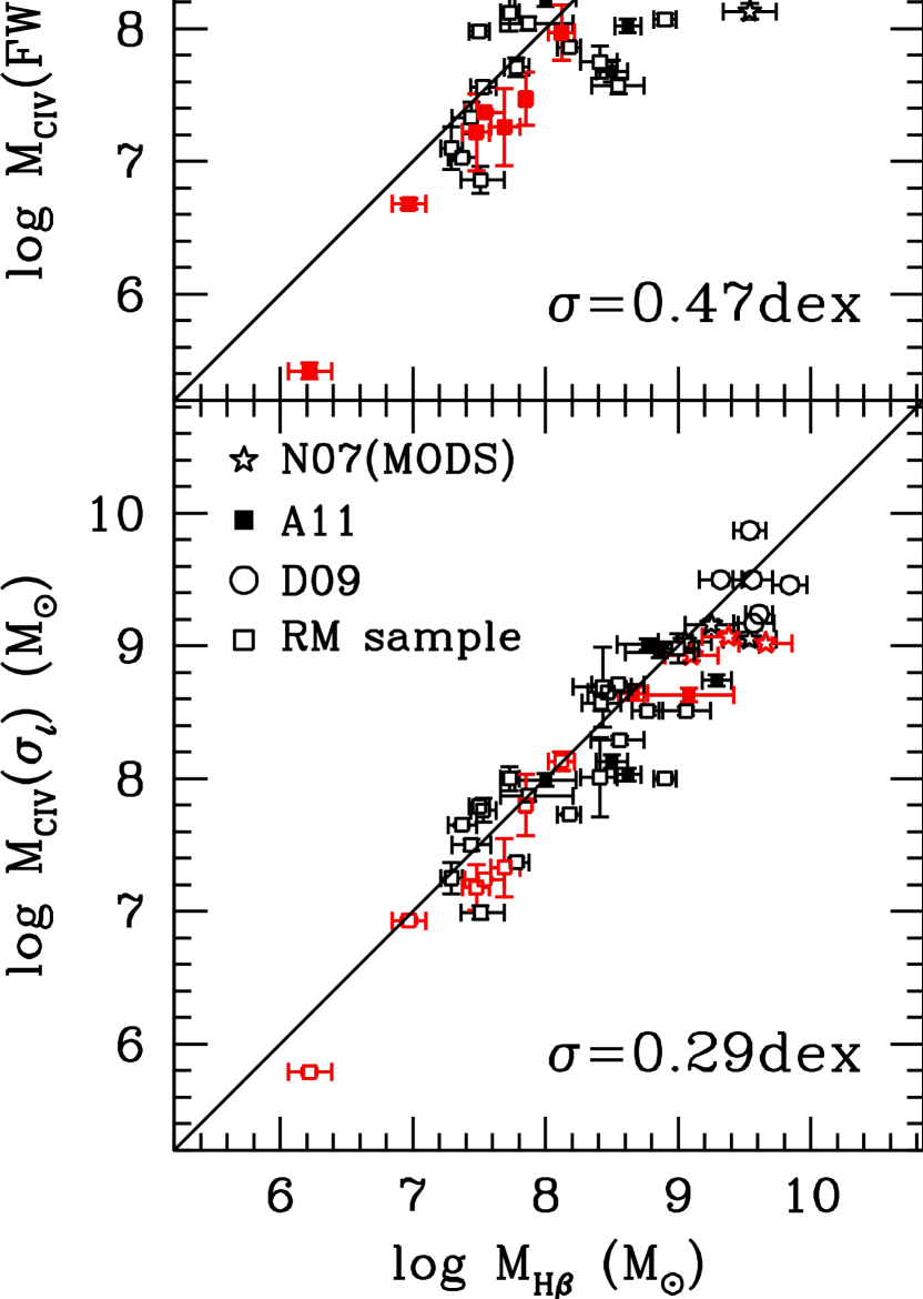
Figure 7.— Comparison between H$\beta$ masses and C iv masses estimated from our complete sample of high quality data. The top (bottom) panel shows C iv masses based on the FWHM ($\sigma_{l}$). The solid line shows where the C iv and H$\beta$ masses are equal. The scatter, $\sigma$, quantified as the standard deviation about the mean of the sample of C iv-to-H$\beta$ mass residuals, $\log M({\rm C}\,{\scriptstyle{\rm IV}})-\log M({\rm H}\beta)$, is shown in the bottom right of each panel. The 12 red points represent objects for which absorption was observed across the peak of the C iv emission line.

6. Discussion

A simple qualitative comparison of the noisy SDSS and MODS1 spectra shown in Figures 3a and 3b clearly demonstrates the deleterious effects low quality data can have on our ability to accurately describe quasar emission line properties. Using this comparison and our results above, we discuss the effects of data quality on characterizing absorption, the C iv velocity width, and SE C iv BH mass estimates.

6.1. Absorption

One striking characteristic of even the small sample of objects observed with both SDSS and MODS1 is the prevalence of narrow absorption features in the C iv profiles. Because C iv $\lambda 1549$ is a resonance transition, self-absorption is common ($>$50%), and it is usually in the form of narrow absorption lines (NALs) due to gas associated with the quasar and/or along the line of sight (e.g., Vestergaard, 2003; Wild et al., 2008; Gibson et al., 2009; Hamann et al., 2011). Recognizing the presence and extent of NAL features in low quality data with a high level of confidence is difficult or impossible. This was demonstrated by A11 for another of the N07 targets (SDSS1151+0340) where an absorption feature was missed in the SDSS spectrum. We see here that the opposite is also possible, as we misidentified noise in the SDSS spectrum of J0254 (Figure 3a, top left) near 1510Å and 1515Å as absorption, and our fit was affected by this assumption. Correctly identifying and modeling intrinsic absorption is absolutely necessary for measuring accurate C iv BH masses.

With high $S/N$ and relatively high spectral resolution data, where the presence of absorption can be accurately detected, the absorption features can usually be masked and interpolated across with relatively few consequences for the line widths and masses. However, when the absorption occurs at the peak of the C iv emission line, it is difficult to know how well an arbitrarily defined profile based on a functional fit reproduces the intrinsic emission-line profile and peak amplitude. There is simply no a priori expectation for the detailed line shapes of individual AGNs. We have marked objects with absorption observed across the C iv emission line peak as red points in Figure 7 to show the possible contribution of line peak absorption to the observed scatter in the masses. We find that the distribution of objects with absorbed peaks is not systematically different that of the unabsorbed objects with respect to the mean C iv to H$\beta$ mass ratio, and the scatter in the C iv to H$\beta$ mass residuals found for our sample actually marginally increases upon omission of these objects from the full sample, from 0.47 to 0.49  dex and 0.29 to 0.30  dex for FWHM- and $\sigma_{l}$-based C iv masses, respectively.

The change in scatter after omitting the 12 absorbed-peak objects is small and could simply be due to small number statistics. In general, however, masses estimated from absorbed-peak profiles using $\sigma_{l}$ will be less prone to biases in the width measurement than FWHM-based mass estimates, because of the relative insensitivity of the line dispersion measurement to the profile peak amplitude. In contrast, absorption and the resulting interpolation uncertainties across the profile peak is more likely to bias FWHM measurements, which are very sensitive to the amplitude of the emission-line peak. A likely explanation for the lack of additional scatter (and even a slight reduction in the scatter) in the masses because of absorbed-peak objects, here, is that the C iv line peak is already contaminated by the non-variable emission component described by Denney (2012). Interpolating over the absorbed peak with Gaussian or Gauss-Hermite functions is more likely to underestimate than overestimate the peak amplitude (Denney et al., 2009a), particularly for the relatively more contaminated, ‘peaky’ C iv profiles. This would, fortuitously, reduce the contamination of this component to the width measurement, leading, in these random cases, to a more accurate C iv mass estimate. This should be the case, in general, but is even more likely to occur with FWHM-based masses, and we do measure the marginally larger difference in scatter in the FWHM-based masses between inclusion or omission of the absorbed-peak objects.

6.2. Line Profile and Width Characterization

The reliability of C iv masses has been debated in the literature not only as a result of the large scatter typically observed between C iv and H$\beta$ masses themselves, but also because of the lack of correlation observed between C iv line widths and those of other broad emission lines (see, e.g., Baskin & Laor, 2005; Ho et al., 2012; Shen & Liu, 2012; Trakhtenbrot & Netzer, 2012). The closed points in the left panel of Figure 8 shows a similar result from our own data. Here we have used the H$\beta$ line widths from Collin et al. (2006) for the mean spectrum of the RM sample objects in order to be more consistent with using a SE C iv line width. Also, we adopt the mean and standard deviation of the C iv FWHM for objects with more than one epoch of data. In general, the C iv line width is expected to be broader than H$\beta$ because of the ionization stratification of the BLR. However, the values shown in the left panel of Figure 8 scatter both above and below the line of equal C iv and H$\beta$ widths. This indicates that characterizing the high-ionization BLR gas velocity using the C iv FWHM from a SE spectrum does not support the physical, virial expectations from an ionization-stratified BLR under the gravitational influence of the BH. On the other hand, the open points compare the C iv and H$\beta$ FWHM measured in the rms spectrum and taken from Denney (2012) and Collin et al. (2006) for each line, respectively, for the six objects that have both C iv and H$\beta$ RM measurements: 3c390.3, Fairall 9, NGC 3783, NGC 4151, NGC  7469, and NGC 5548 (for which we have two independent measurements of both C iv and H$\beta$). When sampling only the reverberating gas velocities, the expectation from a virialized and ionization stratified BLR holds for all objects but Fairall 9, but in this case, the rms C iv profile is weak and likely contaminated by noise, so the FWHM measurement should not be trusted (see Rodriguez-Pascual et al., 1997; Denney, 2012).

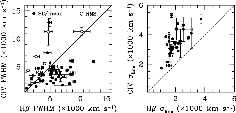
Figure 8.— Left: Comparison between C iv and H$\beta$ FWHM measurements. Right: Comparison between C iv and H$\beta$ $\sigma_{l}$ measurements for objects where H$\beta$ $\sigma_{l}$ was available.

Similar studies in the literature have exclusively focused on comparing FWHM measurements. However, the right panel of Figure 8 shows a similar width comparison using the line dispersion to characterize both the H$\beta$ and C iv line widths for the objects with available H$\beta$ $\sigma_{l}$ measurements. In this case, the relation between C iv and H$\beta$ velocities do follow the virial expectation, even with using the SE line widths: the C iv line widths are exclusively larger than the H$\beta$ widths. Note, however, that a tight correlation is not necessarily expected here because the C iv and H$\beta$ widths are not measured from simultaneous epochs; intrinsic variability creates scatter, since virial expectations imply $\Delta V\propto L^{-1/4}$, and $\Delta L(t)$ is significant ($>$1 dex) for some of the RM sample objects between the C iv and H$\beta$ observations. The level of scatter in Figure 8 is therefore likely inflated, compared to typical expectations for high-$L$ QSOs, because the sample is dominated by the lower-luminosity, more variable RM sample. An additional consideration is that the ratio between the C iv and H$\beta$ velocity widths may depend on the specifics of the BLR structure and accretion rate, leading to some intrinsic scatter between objects. RM time delays for the few objects with both H$\beta$ and C iv results show that the C iv response is typically $2-3$ times shorter than the H$\beta$ response, and the lag and line width follow virial expectations (Peterson & Wandel, 2000; Peterson et al., 2004), but this sample consists of only a handful of intermediate luminosity AGNs.

An additional argument against using the FWHM to derive SE C iv masses was presented by Denney (2012) and follows from the results in the left panel of Figure 8. Denney (2012) demonstrated that there is an emission component in the SE C iv profile that is non-variable and therefore does not seem to be emitted from the same velocity distribution of BLR gas that reverberates in response to the continuum emission. This non-variable component is likely responsible for the ‘peaky’ low-velocity core seen in many C iv profiles (although the non-variable emission may also be present in an additional, or alternate, blue-shifted, broader component). Its presence can significantly contaminate the BLR velocity width measurement when characterizing the SE C iv line profile with the FWHM. This bias is likely responsible for much of the excess scatter seen in our sample when using the FWHM to derive C iv masses and explains why the C iv FWHM measured from the SE spectrum is often narrower than the H$\beta$ FWHM (although Figure 8 demonstrates the same is not true when using the rms spectrum where this component is not present). Thus, despite the problem of absorption, it appears that data quality is not the leading cause of scatter between FWHM-based BH mass measurements, though there is some effect (see Figure 6 and Denney et al. 2009a).

The line dispersion, $\sigma_{l}$, is not as sensitive to the line peak as the FWHM and is therefore less affected by any contamination from the non-variable C iv emission component (although strictly speaking, there must be an effect on some level). The additional insensitivity of $\sigma_{l}$ to absorption in the line peak is another advantage of this line width characterization. However, $\sigma_{l}$ is sensitive to correctly characterizing the wings of the lines, and as such, is very sensitive to $S/N$. In low $S/N$ spectra, it is difficult, if not impossible, to accurately define the boundaries of the emission line and characterize the intrinsic line shape as it merges with a noisy continuum level. A comparison between the SDSS and MODS1 spectrum of J2102 shown in Figure 3b clearly demonstrates the improved clarity with which the wings and extent of the C iv profile can be distinguished from the continuum in high $S/N$ data as opposed to survey-quality data. Unfortunately, the limiting $S/N$ required to accurately trace the intrinsic profile is somewhat dependent on the C iv line shape. The more ‘boxy’, low equivalent width profiles, such as J1055 and J1537, can be more accurately fit in lower $S/N$ data than the ‘peaky’, extended-wing profiles like J2102 because of the relative extension and contrast of the wings compared to the noise level in the continuum.

Mass estimates based on $\sigma_{l}$ are clearly superior to those based on the FWHM with the caveat that $\sigma_{l}$ is sensitive to blending in the line wings, so high quality data are required. This can be a significant source of bias in using $\sigma_{l}$ for H$\beta$ widths (Denney et al., 2009a). This could be a source of bias for C iv as well, as the source of the blended red shelf emission is still uncertain, and misattributing the origin of this emission could bias the resulting C iv $\sigma_{l}$ measurement (see Fine et al., 2010; Assef et al., 2011). Nonetheless, applying a homogeneous spectral decomposition and line width measurement procedure to measure $\sigma_{l}$ can produce consistent $\sigma_{l}$ measurements that lead to little scatter in C iv mass estimates as compared to H$\beta$. As usual, care must be taken in combining samples in order to mitigate scatter resulting from the use of different methodology.

6.3. Black Hole Masses

Higher data quality makes a clear positive impact on the consistency between SE C iv and H$\beta$ BH masses when using the line dispersion to characterize the C iv velocity field. This is demonstrated by the significant reduction in scatter between the low (SDSS) and high (MODS1) quality $\sigma_{l}$-based C iv masses of the N07 sample (see Section 5 and Figure 6). Furthermore, the scatter of only 0.29 dex between the C iv $\sigma_{l}$-based masses and H$\beta$ masses, measured across our full sample of high quality data shown in Figure 7, is arguably the lowest so far quoted in the literature between C iv and H$\beta$ masses for a sample this size, particularly since this (1) does not depend on any type of empirical, potentially sample-dependent, correction, (2) does not factor in the evidence from A11 that a continuum color correction is a comparable contributor to this scatter, and (3) does not take into account inhomogeneities in how the H$\beta$ line widths were measured or other systematics that may be associated with the H$\beta$ mass estimates, which is outside the scope of this work. Another relatively direct piece of evidence for the ability of data quality to reduce the scatter between $\sigma_{l}$-based C iv masses is to look at the RM sample. We measure this scatter to be 0.28 dex in our high-quality RM sample. VP06, whose sample largely overlaps with our own but is more heterogeneous in quality, quote a scatter of 0.37 dex when using weighted averages of the multiple SE C iv masses and H$\beta$ RM campaign masses. The difference between our results and that of VP06 is due in part to data quality differences (see also discussion by Denney, 2012). There are also differences in our spectral analysis and line width measurement methods compared to those of VP06 that may contribute to the reduced scatter. We have learned a lot about the sources of systematic problems in line width measurements since the VP06 study (e.g., Denney et al., 2009a; Fine et al., 2010), so it is not surprising that our reanalysis of this sample has fewer systematic problems.

Conversely, when considering FWHM-based SE C iv mass estimates, our results indicate that obtaining high quality data only marginally improves the consistency between C iv and H$\beta$ SE mass estimates. Figure 6 shows a consistently large scatter between H$\beta$ and FWHM-based C iv masses for both low and high quality data, and our results from the top panel of Figure 7 including the full sample of high-quality data corroborate this finding. We can again make a comparison to the VP06 results for the RM sample to look at the differences in scatter between our high-quality data set and their heterogeneous-quality data set. VP06 quote a scatter of 0.43 dex, while we find a scatter of 0.36 dex. There is some improvement, but again prescriptional differences could play a part in this difference as well.

Finally, it is still difficult with our sample to address the concerns of Richards et al. (2011) regarding the applicability of existing C iv SE mass scaling relationships to quasars covering the complete C iv EQW–blueshift parameter space observed for SDSS quasars. While our sample covers more than an order of magnitude in C iv EQWs, we still only have one source with a low C iv EQW and a large C iv blueshift (see Figure 2). This is Q2302 from the D09 sample, and it is the object found to have the largest estimated C iv mass in our sample. Q2302 does appear as a significant outlier in the top panel of Figure 7 when its mass is estimated using the C iv FWHM, again suggesting that FWHM-based C iv masses may less reliable, but it is no larger an outlier than other sources without large C iv blueshifts. When the C iv mass is estimated with $\sigma_{l}$, it also falls within the same, albeit much smaller, range of scatter as the rest of the sample. More low C iv EQW–large blueshift objects should be specifically targeted for both SE mass comparisons and RM studies to be able to address this concern further.

6.4. C IV Mass Scale Calibration

The analysis and results presented above are based on the C iv mass scale calibrated by VP06. After completion and initial submission of this current work, an updated calibration of the C iv mass scale became available (Park et al., 2013, hereafter P13). The new calibration of P13 differs from that of VP06 in two main respects: P13 (1) incorporates the most up-to-date database of high quality HST spectra of the reverberation mapping sample (essentially the same sample we use here), while excluding low quality spectra altogether, and (2) relaxes the $M\propto V^{2}$ virial expectation, which improves the empirical calibration of the FWHM-based C iv masses (see P13 for details). We have recalculated our C iv masses using the P13 C iv mass scaling relationships to evaluate if the consistency between C iv and H$\beta$ masses improves with these updated C iv mass scaling relations. Figure 9 shows the comparison of C iv and H$\beta$ masses that is equivalent to Figure 7 but using Equations (2) and (3) of P13.

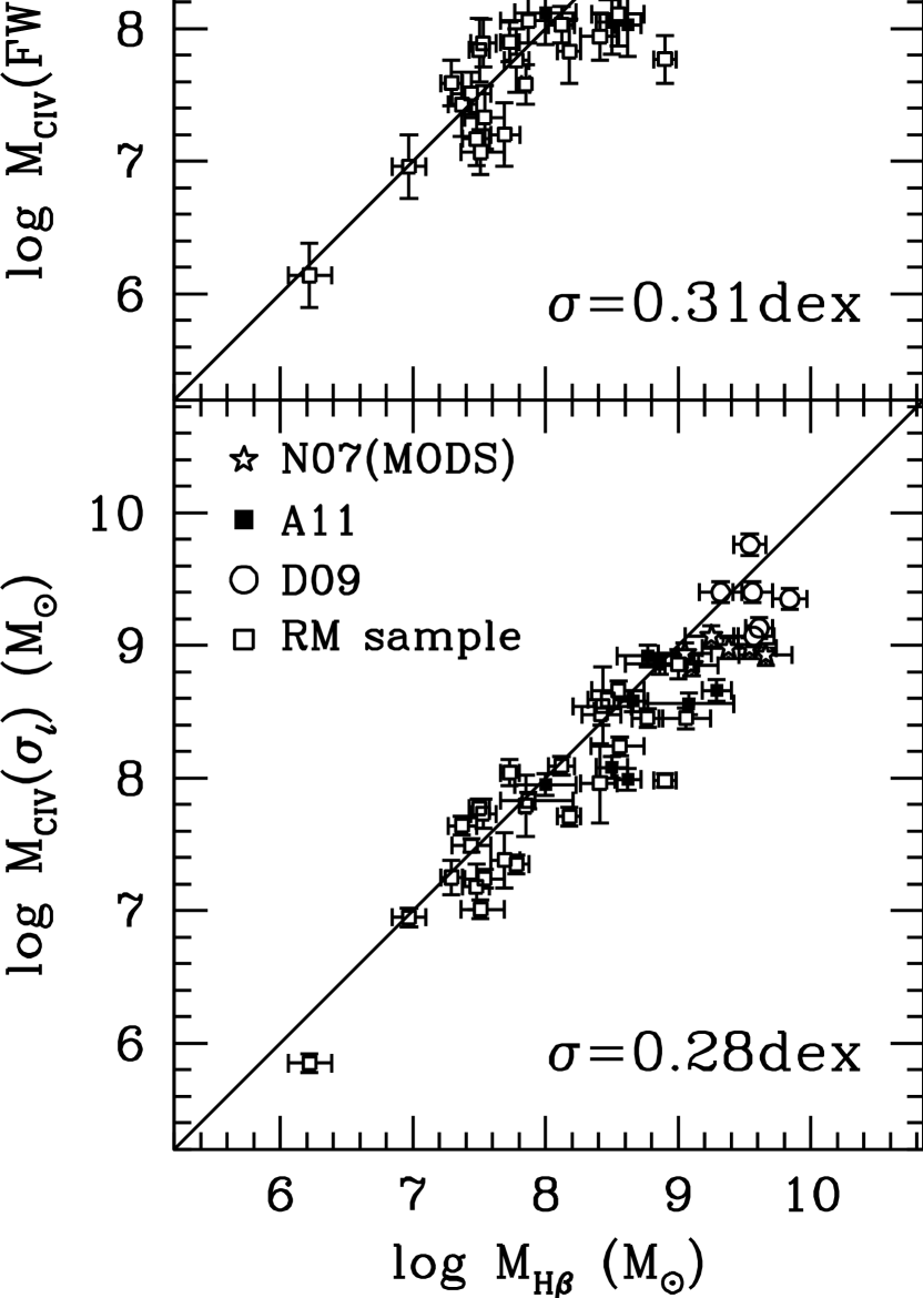
Figure 9.— Comparison between H$\beta$ masses and C iv masses estimated from our complete sample of high quality data using the new C iv mass scaling relationships of P13. The top (bottom) panel shows C iv masses based on the FWHM ($\sigma_{l}$). The solid line shows where the C iv and H$\beta$ masses are equal. The scatter, $\sigma$, quantified as the standard deviation about the mean of the sample of C iv-to-H$\beta$ mass residuals, $\log M({\rm C}\,{\scriptstyle{\rm IV}})-\log M({\rm H}\beta)$, is shown in the bottom right of each panel.

The most significant difference between our previous results and those utilizing these updated C iv mass scale calibrations is that the scatter between the C iv FWHM-based masses and the H$\beta$ masses is significantly smaller. This is a consequence of the $M_{{\rm C}\,{\scriptstyle{\rm IV}}}(\rm FWHM)$ dependence on $V^{0.56}$ instead of the virial expectation of $V^{2}$, which helps to correct for line width dependent biases; it effectively applies a line-width dependent scale factor to the masses (see Wang et al., 2009; Rafiee & Hall, 2011a, for similarly justified re-calibration of the Mg ii FWHM-based SE mass scale). For C iv this corrects for the varying amounts of contamination by the non-variable C iv emission component, which is a function of the C iv FWHM (see Denney, 2012). Such an empirical calibration may be the answer for survey quality data, from which a measurement of the FWHM is easier to make and more robust than $\sigma_{l}$ to $S/N$, but this type of calibration is strongly sample dependent, particularly on the distribution of C iv line shapes present in the calibration sample, and the RM sample is relatively small and not yet representative of the overall quasar population in this respect, so caution interpreting the results of its application is necessary. P13 find that a similar relaxation of the virial dependence for $\sigma_{l}$-based C iv masses is not warranted, and the P13 calibration for $\sigma_{l}$-based C iv masses is very similar to the VP06 calibration. We do not see any significant improvement in the consistency between the $\sigma_{l}$-based C iv and H$\beta$ masses using the new calibration; the scatter was unaffected. This demonstrates that $\sigma_{l}$ based masses continue to more consistently reproduce H$\beta$-based BH masses with continued evidence for a virial relation between the velocity dispersion of the gas measured with $\sigma_{l}$ and the black hole mass.

A notable zero-point offset remains between the unity relation of the C iv and H$\beta$ mass and the distribution of points shown in Figure 9. We attributed the offset observed in Figure 7 largely to prescriptional differences in the line width measurements between our study and that of VP06. However, we use a prescription for fitting the spectra and measuring the line widths that is very similar to P13. We have confirmed that this is not the source of the offset here by comparing the line width measurements from data we have in common with P13 (e.g., individual COS spectra of the RM sample). Instead, we traced the source of the offset to the luminosity measurements. For the RM sample shared by both studies, we find that the mass offset between the P13 C iv masses and our own can be explained by (1) a minimal number of outliers resulting from large luminosity differences because of the distance to these objects (NGC4151, NGC4593, NGC4051, and NGC3873) adopted here and by P13: P13 used the published redshifts to determine the luminosity, while we used the best estimate of the distance measured from direct measurement methods (see Bentz et al., 2013, for details), (2) small, but significant differences between L1350 and L1450 in another small subset of targets with a relatively steeper UV continuum slope (despite direct comparisons and a statement of general equivalence by both VP06 and P13), and (3) intrinsic variability, which introduces luminosity differences for individual objects because of the different method P13 used to combine multiple SE spectra of a single object compared to the procedure we used here. In all but one case (NGC4051), the former two contributors lead to our C iv masses being lower than those estimated by P13. The fact that the final contributor led to overall systematically lower C iv masses is serendipitous. In any case, the resulting zero-point offsets in our masses, while not impacting our main results here, underscores the importance for making direct measurements of the C iv-emitting radius of the BLR with reverberation mapping, so that C iv masses can be calibrated directly from a C iv $R-L$ relationship. Such a calibration would be independent of the intrinsic variability effects in the current calibration that are also the hardest of the above contributors to mitigate.

7. Summary and Concluding Remarks: Overall Impact of Data Quality

We have presented LBT/MODS1 spectra of the C iv emission line of six high-redshift quasars that previously only had SDSS spectra. We expanded this small sample with 41 additional homogeneously re-analyzed, high $S/N$ ($\geq$10 pixel^-1 in the continuum) spectra of the C iv emission-line region from the literature or public archives. The most significant improvements afforded by the increased data quality in the MODS1 spectra over that of survey-quality data is the increased ability to accurately define the intrinsic C iv emission-line profile and underlying continuum and accurately identify the prevalence, location, and strength of absorption. With the advantage the data quality lends to accurately characterizing the C iv line profile, SE C iv BH masses can reliably be estimated from the virial relation using high-quality data — but only when using the line dispersion, $\sigma_{l}$, to characterize the C iv emission-line width (Figure 7). The converse is true as well: SE C iv masses can be reliably estimated with $\sigma_{l}$, but only using high $S/N$ spectra (Figure 6). The scatter, quantified as the standard deviation about the mean of the residuals between the H$\beta$ and $\sigma_{l}$-based C iv masses, decreased by a factor of 2 (to 0.24 dex) between results based on survey-quality SDSS spectra and high $S/N$ MODS1 spectra for an, albeit, small sample of AGNs. Similarly, however, the same measure of scatter in our full sample of 47 objects with high quality spectra was only 0.29 dex. Conversely, data quality had little impact on the scatter between H$\beta$ and FWHM-based C iv masses for our sample. This implies that obtaining high $S/N$ data cannot improve FWHM-based C iv masses the same way it can improve $\sigma_{l}$-based C iv masses. Instead, it is possible that much of the scatter between FWHM-based C iv and H$\beta$ masses is due to the presence of the non-variable C iv emission component described by Denney (2012). This component significantly biases the BLR velocity measurement when the FWHM is used. C iv masses based on the FWHM of the line profile and a virial mass estimation should therefore not be used.

An alternative is to apply empirical corrections to survey quality, FWHM-based mass estimates. Denney (2012) provide an empirical correction for FWHM-based C iv masses based on the “shape” of the C iv line. Denney (2012) parameterized the line shape as the ratio of the FWHM to $\sigma_{l}$ and found it to correlate with the C iv-to-H$\beta$ mass residuals. However, since characterizing the line shape this way requires a measurement of $\sigma_{l}$ anyway, one could simply employ a $\sigma_{l}$-based C iv mass and avoid the need for a correction altogether. Measuring the shape from the kurtosis of the line also produces a similar correlation with the C iv-to-H$\beta$ mass residuals, but regardless, accurately characterizing the line shape with any parameterization is data-quality dependent, so this type of correction is not likely to be as effective for survey quality data. Alternately, the new empirically calibrated FWHM-based C iv mass scaling relationship of P13 relaxes the virial assumption between the FWHM and the BH mass in order to mitigate biases in the BH mass due to the C iv FWHM measurement. This reduces scatter between the C iv and H$\beta$ masses but removes much of the connection to the physical assumptions behind virial BH mass estimators and will still have some dependence on data quality — both the current and P13 data sets were high $S/N$, but Denney et al. (2009a) describes reasonable expectations for the effects the reduced $S/N$ of survey data may have on the dispersion in the mass distribution. Future work is planned to improve the effectiveness of corrections for survey-quality FWHM-based masses (see also Runnoe et al., 2013). As with any correction of this type, the potential for sample bias in the calibration is an issue, but such a correction has the potential to improve C iv masses estimated from survey-quality data at least somewhat.

A11 also provide a correction to C iv SE masses based on the ratio of UV-to-optical luminosities. Trakhtenbrot & Netzer (2012) argue that such a correlation is not broadly applicable because the rest frame optical luminosity is rarely available for high-$z$ quasar samples. Nonetheless, it is the implication behind the A11 correction that is of the most interest for the C iv-based mass debate — UV-to-optical luminosity differences may be as much of a source of scatter in the comparison of C iv-to-H$\beta$ BH masses as the measurement of $\Delta V$, implying that it is not specifically (or only) the C iv emission line that is to blame for the observed discrepancies.

In the end, reliably determining C iv BH masses is of significant interest to the larger astronomical community, since these masses are essential for studying the cosmic evolution and growth of BHs and their connection to galaxy evolution (e.g., feedback). Even modest improvements in precision and accuracy of BH mass estimates are a step in the right direction and can add at least some additional constraints to theoretical and model- or simulation-based studies of cosmological evolution that depend on BH mass and growth rates. Compared to all other literature studies of this size and type, the relatively smaller scatter observed here for the $\sigma_{l}$-based SE C iv masses, 0.28  dex, by using only high quality data implies that the best-achievable precision in SE mass estimates is higher than previously believed. In particular, we fit the distribution of $\sigma_{l}$-based C iv masses shown in Figure 9 with the IDL program MPFITEXY to estimate the intrinsic scatter of the C iv masses compared to the H$\beta$ masses, by taking into account the measurement and mass scale calibration uncertainties. By holding the slope fixed to a unity relation between the C iv and H$\beta$ mass, we find an estimate of the intrinsic scatter of these high quality $\sigma_{l}$-based C iv masses to be 0.22  dex; that for the FWHM-based C iv masses is similar, 0.21  dex. This is on order the observed scatter in the $R-L$ relationship on which the foundation of SE mass estimates is built (see Bentz et al., 2013). Future work is planned to investigate additional applications of these results to better understand the remaining scatter between C iv and H$\beta$ masses. The potential for further reduction in the observed scatter between these two quantities is promising, but we may be close to the limit of what is possible for this method unless scatter in the $R-L$ relationship can be further reduced. Nonetheless, the application of such results to studies of AGN physics and galaxy evolution will require larger samples of high quality quasar spectra or development of new techniques that can reliably characterize the BLR velocity from current survey quality spectra.

Table 1Journal of Observations

Object	z	UTC Date	Exposures	Channel	Grating	Seeing	Notes
SDSSJ025438.37+002132.8	2.456	2011 Sept 28	3$\times$500s	Blue	G400L	0$\farcs$6	Thin Cirrus
SDSSJ105511.99+020751.9	3.391	2012 Mar 23	3$\times$1600s	Red	G670L	0$\farcs$6	Clear
SDSSJ115935.64+042420.0	3.451	2012 Apr 30	3$\times$1200s	Red	G670L	0$\farcs$6	Clear
SDSSJ153725.36-014650.3	3.452	2012 Mar 24	3$\times$1800s	Red	G670L	0$\farcs$6	Patchy clouds; wind
SDSSJ210258.22+002023.4	3.328	2011 Sept 28	3$\times$1300s	Red	G670L	0$\farcs$7	Moderate Cirrus
SDSSJ210311.68-060059.4	3.336	2011 Sept 27	4$\times$250s	Red	G670L	0$\farcs$7	Thin Cirrus

Table 2N07 Sample Spectral Properties, Luminosities, and BH Masses

Property	J0254	J1055	J1159	J1537	J2102	J2103
SDSS Spectra
$S/N$	8.0	8.4	11.1	4.8	4.5	9.6
C iv Obs. Line Boundaries (Å)	5150–5600	6500–7100	6535–7200	6565–7030	6400–6950	6470–6930
C iv FWHM(N07; km s-1)	4753	5476	4160	5650	2355	4951
C iv FWHM(this study; km s-1)	3170$\pm$250	5680$\pm$620	3250$\pm$390	5980$\pm$1250	1340$\pm$840	2850$\pm$170
C iv $\sigma_{l}$(this study; km s-1)	2930$\pm$140	4100$\pm$130	4110$\pm$110	3910$\pm$720	2260$\pm$280	2960$\pm$130
log $\lambda L_{\lambda}$(1450Å)(erg s-1)	45.93	46.24	46.43	46.44	45.86	46.24
log $M_{{\rm C}\,{\scriptstyle{\rm IV}}}$(FWHM)(M⊙)	8.69$\pm$0.08	9.36$\pm$0.10	8.97$\pm$0.11	9.51$\pm$0.19	7.90$\pm$0.55	8.76$\pm$0.07
log $M_{{\rm C}\,{\scriptstyle{\rm IV}}}$($\sigma_{l}$)(M⊙)	8.69$\pm$0.06	9.14$\pm$0.05	9.25$\pm$0.05	9.21$\pm$0.17	8.42$\pm$0.12	8.86$\pm$0.04
MODS Spectra
$S/N$	17.8	80.4	50.5	51.9	31.3	47.3
C iv Line Boundaries (Å)	5100–5600	6515–7070	6665–7180	6585–7180	6300–6950	6470–6930
C iv FWHM (km s-1)	2440$\pm$100	4980$\pm$180	2130$\pm$80	4910$\pm$170	1750$\pm$70	3120$\pm$70
C iv $\sigma_{l}$ (km s-1)	3870$\pm$40	4170$\pm$30	3350$\pm$40	3200$\pm$50	4660$\pm$80	3560$\pm$30
log $M_{{\rm C}\,{\scriptstyle{\rm IV}}}$(FWHM)(M⊙)	8.46$\pm$0.06	9.24$\pm$0.05	8.61$\pm$0.05	9.34$\pm$0.05	8.13$\pm$0.06	8.84$\pm$0.05
log $M_{{\rm C}\,{\scriptstyle{\rm IV}}}$($\sigma_{l}$)(M⊙)	8.93$\pm$0.04	9.16$\pm$0.04	9.07$\pm$0.04	9.03$\pm$0.05	9.05$\pm$0.05	9.02$\pm$0.04
Gemini Spectra; N07
H$\beta$ FWHM(km s-1)	4164	5424	5557	3656	7198	6075
log $\lambda L_{\lambda}$(5100Å)(erg s-1)	45.85	45.85	45.92	45.98	45.79	46.30
log $M_{{\rm H}\beta}$(FWHM)(M⊙)	9.162	9.294	9.460	9.133	9.599	9.785

Table 3D09 Sample Spectral Parameters and Masses

D09	NED		Res.	C iv Rest Frame	log $\lambda L_{\lambda}$(1350Å)	FWHM(CIV)	$\sigma_{l}$(CIV)	log $M_{{\rm C}\,{\scriptstyle{\rm IV}}}$(FWHM)	log $M_{{\rm C}\,{\scriptstyle{\rm IV}}}$($\sigma_{l}$)	log $M_{{\rm H}\beta}$
Object ID	Object ID	$z$	(Å)	Boundaries	(erg s-1)	(km s-1)	(km s-1)	(M⊙)	(M⊙)	(M⊙)
(1)	(2)	(3)	(4)	(5)	(6)	(7)	(8)	(9)	(10)	(11)
Q 0150-202	[HB89] 0150-202	2.147	2.8	1465–1597	46.970	4230$\pm$310	3790$\pm$100	9.49$\pm$0.08	9.46$\pm$0.05	9.84$\pm$0.13
Q 2116-4439	LBQS 2116-4439	1.504	2.8	1477–1635	46.712	7540$\pm$140	4660$\pm$50	9.85$\pm$0.05	9.50$\pm$0.04	9.32$\pm$0.16
Q 2154-2005	LBQS 2154-2005	2.042	2.8	1490–1625	46.681	5030$\pm$190	3250$\pm$70	9.49$\pm$0.05	9.17$\pm$0.05	9.57$\pm$0.15
Q 2209-1842	LBQS 2209-1842	2.098	2.8	1480–1610	46.808	3020$\pm$100	3230$\pm$50	9.11$\pm$0.05	9.24$\pm$0.05	9.61$\pm$0.10
Q 2230+0232	LBQS 2230+0232	2.215	2.8	1470–1640	46.724	4540$\pm$160	4590$\pm$60	9.42$\pm$0.05	9.50$\pm$0.05	9.56$\pm$0.15
Q 2302+0255	[HB89] 2302+029	1.062	2.8	1440–1610	46.915	12940$\pm$690	6270$\pm$140	10.43$\pm$0.06	9.87$\pm$0.05	9.54$\pm$0.12

Table 4Reverberation Sample H$\beta$ Rest-frame Lags, Line Widths, and Masses

		$\tau_{\rm cent}$	$\sigma_{l}$(RMS)	log $M_{\rm RM}$(H$\beta$)
Object	$z$	Restframe	(km s-1)	(M⊙)	(Ref.)
(1)	(2)	(3)	(4)	(5)	(6)
Mrk 335	0.02578	16.80${}^{+4.80}_{-4.20}$	917$\pm$52	7.16${}^{+0.16}_{-0.15}$	1,25
	0.02578	12.50${}^{+6.60}_{-5.50}$	948$\pm$113	7.06${}^{+0.27}_{-0.24}$	1,25
	0.02578	14.30${}^{+0.70}_{-0.70}$	1293$\pm$64	7.39${}^{+0.10}_{-0.10}$	2
				$7.29^{+0.08}_{-0.08}$
PG0026+129	0.14200	111.00${}^{+24.10}_{-28.30}$	1773$\pm$285	8.55${}^{+0.19}_{-0.20}$	3,25
PG0052+251	0.15500	89.80${}^{+24.50}_{-24.10}$	1783$\pm$86	8.47${}^{+0.15}_{-0.15}$	3,25
Fairall 9	0.04702	17.40${}^{+3.20}_{-4.30}$	3787$\pm$197	8.41${}^{+0.13}_{-0.15}$	4,5,25
Mrk 590	0.02638	20.70${}^{+3.50}_{-2.70}$	789$\pm$74	7.12${}^{+0.14}_{-0.13}$	1,25
	0.02638	14.00${}^{+8.50}_{-8.80}$	1935$\pm$52	7.73${}^{+0.28}_{-0.29}$	1,25
	0.02638	29.20${}^{+4.90}_{-5.00}$	1251$\pm$72	7.67${}^{+0.13}_{-0.13}$	1,25
	0.02638	28.80${}^{+3.60}_{-4.20}$	1201$\pm$130	7.63${}^{+0.14}_{-0.14}$	1,25
				$7.50^{+0.08}_{-0.08}$
3C 120	0.03301	38.10${}^{+21.30}_{-15.30}$	1166$\pm$50	7.73${}^{+0.26}_{-0.20}$	1,25
	0.03301	25.90${}^{+2.30}_{-2.30}$	1514$\pm$65	7.79${}^{+0.10}_{-0.10}$	2
				$7.78^{+0.10}_{-0.09}$
Akn 120	0.03230	47.10${}^{+8.30}_{-12.40}$	1959$\pm$109	8.27${}^{+0.13}_{-0.15}$	1,25
	0.03230	37.10${}^{+4.80}_{-5.40}$	1884$\pm$48	8.13${}^{+0.11}_{-0.11}$	1,25
				$8.18^{+0.08}_{-0.09}$
PG0804+761	0.10000	146.90${}^{+18.80}_{-18.90}$	1971$\pm$105	8.77${}^{+0.12}_{-0.12}$	3,25
PG0953+414	0.23410	150.10${}^{+21.60}_{-22.60}$	1306$\pm$144	8.42${}^{+0.15}_{-0.15}$	3,25
NGC 3516	0.00884	11.68${}^{+1.02}_{-1.53}$	1591$\pm$10	7.48${}^{+0.10}_{-0.11}$	6
NGC 3783	0.00584	10.20${}^{+3.30}_{-2.30}$	1753$\pm$141	7.51${}^{+0.18}_{-0.15}$	7,8,9,25
NGC 4051	0.00397	1.87${}^{+0.54}_{-0.50}$	927$\pm$64	6.22${}^{+0.17}_{-0.16}$	10
NGC 4151	0.0026	6.59${}^{+1.12}_{-0.76}$	2680$\pm$64	7.69${}^{+0.12}_{-0.11}$	11
PG1226+023	0.15834	306.80${}^{+68.50}_{-90.90}$	1777$\pm$150	9.00${}^{+0.15}_{-0.17}$	3,25
PG1229+204	0.06301	37.80${}^{+27.60}_{-15.30}$	1385$\pm$111	7.87${}^{+0.34}_{-0.21}$	3,25
NGC 4593	0.00865	3.73${}^{+0.75}_{-0.75}$	1561$\pm$55	6.97${}^{+0.13}_{-0.13}$	12
PG1307+085	0.15500	105.60${}^{+36.00}_{-46.60}$	1820$\pm$122	8.56${}^{+0.18}_{-0.22}$	3,25
Mrk 279	0.03045	16.70${}^{+3.90}_{-3.90}$	1420$\pm$96	7.54${}^{+0.15}_{-0.15}$	13,25
NGC 5548	0.01717	19.70${}^{+1.50}_{-1.50}$	1687$\pm$56	7.76${}^{+0.10}_{-0.10}$	14,15,16,25
	0.01717	18.60${}^{+2.10}_{-2.30}$	1882$\pm$83	7.83${}^{+0.11}_{-0.11}$	14,25
	0.01717	15.90${}^{+2.90}_{-2.50}$	2075$\pm$81	7.85${}^{+0.12}_{-0.12}$	14,25
	0.01717	11.00${}^{+1.90}_{-2.00}$	2264$\pm$88	7.76${}^{+0.12}_{-0.12}$	14,25
	0.01717	13.00${}^{+1.60}_{-1.40}$	1909$\pm$129	7.69${}^{+0.12}_{-0.12}$	14,17,25
	0.01717	13.40${}^{+3.80}_{-4.30}$	2895$\pm$114	8.06${}^{+0.16}_{-0.17}$	14,25
	0.01717	21.70${}^{+2.60}_{-2.60}$	2247$\pm$134	8.05${}^{+0.12}_{-0.12}$	14,25
	0.01717	16.40${}^{+1.20}_{-1.10}$	2026$\pm$68	7.84${}^{+0.10}_{-0.10}$	14,25
	0.01717	17.50${}^{+2.00}_{-1.60}$	1923$\pm$62	7.82${}^{+0.11}_{-0.10}$	14,25
	0.01717	26.50${}^{+4.30}_{-2.20}$	1732$\pm$76	7.91${}^{+0.12}_{-0.10}$	14,25
	0.01717	24.80${}^{+3.20}_{-3.00}$	1980$\pm$30	8.00${}^{+0.11}_{-0.11}$	14,25
	0.01717	6.50${}^{+5.70}_{-3.70}$	1969$\pm$48	7.41${}^{+0.39}_{-0.26}$	14,25
	0.01717	14.30${}^{+5.90}_{-7.30}$	2173$\pm$89	7.84${}^{+0.20}_{-0.24}$	14,25
	0.01717	6.30${}^{+2.60}_{-2.30}$	3210$\pm$642	7.82${}^{+0.27}_{-0.25}$	18
	0.01717	12.40${}^{+2.74}_{-3.85}$	1822$\pm$35	7.63${}^{+0.13}_{-0.16}$	6
	0.01717	4.18${}^{+0.86}_{-1.30}$	4270$\pm$292	7.89${}^{+0.14}_{-0.17}$	19
				$7.85^{+0.03}_{-0.03}$
PG1426+015	0.08647	95.00${}^{+29.90}_{-37.10}$	3442$\pm$308	9.06${}^{+0.18}_{-0.21}$	3,25
Mrk 817	0.03145	19.00${}^{+3.90}_{-3.70}$	1392$\pm$78	7.58${}^{+0.14}_{-0.13}$	1,25
	0.03145	15.30${}^{+3.70}_{-3.50}$	1971$\pm$96	7.79${}^{+0.14}_{-0.14}$	1,25
	0.03145	33.60${}^{+6.50}_{-7.60}$	1729$\pm$158	8.01${}^{+0.15}_{-0.16}$	1,25
	0.03145	14.04${}^{+3.41}_{-3.47}$	2025$\pm$5	7.77${}^{+0.14}_{-0.14}$	6
				$7.78^{+0.07}_{-0.07}$
Mrk 290	0.02958	8.72${}^{+1.21}_{-1.02}$	1609$\pm$47	7.37${}^{+0.11}_{-0.11}$	6
PG1613+658	0.12900	40.10${}^{+15.00}_{-15.20}$	2547$\pm$342	8.43${}^{+0.22}_{-0.22}$	3,25
3C 390.3	0.05610	23.60${}^{+6.20}_{-6.70}$	3105$\pm$81	8.37${}^{+0.15}_{-0.15}$	20,21,25
	0.05610	46.40${}^{+3.60}_{-3.20}$	5455$\pm$278	9.15${}^{+0.11}_{-0.10}$	22
				$8.90^{+0.09}_{-0.09}$
Mrk 509	0.03440	79.60${}^{+6.10}_{-5.40}$	1276$\pm$28	8.12${}^{+0.10}_{-0.10}$	1,25
PG2130+099	0.06298	22.90${}^{+4.70}_{-4.60}$	1246$\pm$222	7.56${}^{+0.20}_{-0.20}$	23
	0.06298	9.60${}^{+1.20}_{-1.20}$	1825$\pm$65	7.52${}^{+0.11}_{-0.11}$	2
				$7.53^{+0.10}_{-0.10}$
NGC 7469	0.01632	16.50${}^{+2.90}_{-2.90}$	1274$\pm$126	7.44${}^{+0.15}_{-0.15}$	24

References. — (1)Peterson et al. (1998); (2)Grier et al. (2012); (3)Kaspi et al. (2000); (4)Santos-Lleó et al. (1997); (5)Rodriguez-Pascual et al. (1997); (6)Denney et al. (2010); (7)Stirpe et al. (1994); (8)Onken & Peterson (2002); (9)Reichert et al. (1994); (10)Denney et al. (2009b); (11)Bentz et al. (2006); (12)Denney et al. (2006); (13)Santos-Lleó et al. (2001); (14)Peterson et al. (2002, and references therein); (15)Dietrich et al. (1993); (16)Clavel et al. (1991); (17)Korista et al. (1995); (18)Bentz et al. (2007); (19)Bentz et al. (2009b); (20)Dietrich et al. (1998); (21)O’Brien et al. (1998); (22)Dietrich et al. (2012); (23)Grier et al. (2008); (24) Peterson et al. (2013, in prep.); (25)Reanalyzed by Peterson et al. (2004).

Table 5Reverberation Sample C iv Spectral Parameters and Masses

		Date	Telescope/	Resolution	C iv Obs. Frame	log $\lambda L_{\lambda}$(1450Å)	FWHM(CIV)	$\sigma_{l}$(CIV)	log $M_{{\rm C}\,{\scriptstyle{\rm IV}}}$(FWHM)	log $M_{{\rm C}\,{\scriptstyle{\rm IV}}}$($\sigma_{l}$)
Object	$z$	Observed	Instrument	(Å)	Boundaries	(erg s-1)	(km s-1)	(km s-1)	(M⊙)	(M⊙)
(1)	(2)	(3)	(4)	(5)	(6)	(7)	(8)	(9)	(10)	(11)
Mrk 335	0.02578	1994 Dec 16	HST/FOS	1.40	1553–1625	44.129$\pm$0.002	2000$\pm$60	2020$\pm$20	7.33$\pm$0.03	7.41$\pm$0.01
	0.02578	2009 Oct 31	HST/COS	0.21	1550–1635	43.850$\pm$0.001	1730$\pm$30	1880$\pm$10	7.06$\pm$0.02	7.20$\pm$0.01
	0.02578	2010 Feb 8	HST/COS	0.21	1550–1635	43.850$\pm$0.001	1690$\pm$30	1860$\pm$10	7.04$\pm$0.02	7.19$\pm$0.01
									$7.10\pm 0.16$	$7.25\pm 0.12$
PG0026+129	0.14200	1994 Nov 27	HST/FOS	1.40	1660–1870	45.007$\pm$0.004	1540$\pm$110	5310$\pm$130	7.57$\pm$0.06	8.71$\pm$0.02
PG0052+251	0.15500	1993 July 22	HST/FOS	2.20	1690–1880	45.064$\pm$0.006	5710$\pm$370	4740$\pm$80	8.74$\pm$0.06	8.65$\pm$0.02
Fairall 9	0.04702	1994 RM	IUE/SWP	6.00	1535–1670	44.479$\pm$0.003	2830$\pm$60	4080$\pm$40	7.82$\pm$0.02	8.21$\pm$0.01
	0.04702	1993 Jan 22	HST/FOS	2.20	1560–1680	44.360$\pm$0.004	2510$\pm$70	2710$\pm$30	7.65$\pm$0.03	7.79$\pm$0.01
									$7.75\pm 0.12$	$8.01\pm 0.30$
Mrk 590	0.02638	1991 Jan 14	IUE/SWP	6.00	1520–1670	43.961$\pm$0.009	4690$\pm$230	3480$\pm$80	7.98$\pm$0.04	7.79$\pm$0.02
3C 120	0.03301	1993 Aug 25	IUE/SWP	6.00	1570–1645	43.959$\pm$0.008	3450$\pm$270	2150$\pm$60	7.71$\pm$0.07	7.37$\pm$0.03
Akn 120	0.03230	1995 Jul 29	HST/FOS	1.40	1545–1655	44.038$\pm$0.004	3900$\pm$130	3090$\pm$30	7.86$\pm$0.03	7.73$\pm$0.01
PG0804+761	0.10000	2010 Jun 12	HST/COS	2.10	1640–1770	45.396$\pm$0.001	3630$\pm$130	3320$\pm$70	8.52$\pm$0.03	8.51$\pm$0.02
PG0953+414	0.23410	1991 Jun 17	HST/FOS	1.50	1850–1980	45.587$\pm$0.003	2860$\pm$100	3230$\pm$40	8.41$\pm$0.03	8.59$\pm$0.01
	0.23410	2001 Jan 21	HST/STIS	3.14	1840–1980	45.650$\pm$0.005	2900$\pm$120	2830$\pm$80	8.46$\pm$0.04	8.51$\pm$0.03
									$8.43\pm 0.04$	$8.57\pm 0.06$
NGC 3516	0.00884	1995 Dec 30	HST/FOS	1.40	1475–1620	42.671$\pm$0.003	3050$\pm$90	3460$\pm$40	6.92$\pm$0.03	7.10$\pm$0.01
	0.00884	1996 Feb 21	HST/FOS	1.40	1475–1620	43.038$\pm$0.002	4750$\pm$160	3490$\pm$50	7.50$\pm$0.03	7.31$\pm$0.02
	0.00884	1996 Apr 13	HST/FOS	1.40	1475–1620	42.990$\pm$0.002	3850$\pm$150	3250$\pm$40	7.30$\pm$0.04	7.22$\pm$0.01
	0.00884	1996 Aug 14	HST/FOS	1.40	1475–1620	42.869$\pm$0.002	4130$\pm$90	3380$\pm$40	7.29$\pm$0.02	7.19$\pm$0.01
	0.00884	1996 Nov 28	HST/FOS	1.40	1475–1630	42.345$\pm$0.005	2990$\pm$100	3170$\pm$40	6.73$\pm$0.03	6.85$\pm$0.02
	0.00884	1998 Apr 13	HST/STIS	1.20	1475–1640	42.659$\pm$0.002	4890$\pm$80	4480$\pm$20	7.33$\pm$0.02	7.32$\pm$0.01
									$7.22\pm 0.29$	$7.18\pm 0.17$
NGC 3783	0.00584	1992 RM	IUE/SWP	6.00	1520–1610	42.702$\pm$0.003	2900$\pm$60	2860$\pm$20	6.90$\pm$0.02	6.95$\pm$0.01
	0.00584	1992 Jul 22	HST/FOS	1.95	1520–1630	42.854$\pm$0.002	2270$\pm$80	2830$\pm$20	6.76$\pm$0.03	7.03$\pm$0.01
									$6.86\pm 0.10$	$6.99\pm 0.05$
NGC 4051	0.00397	2000 Mar 25	HST/STIS	0.51	1520–1585	41.796$\pm$0.004	1220$\pm$90	1730$\pm$30	5.66$\pm$0.06	6.04$\pm$0.02
NGC 4151	0.0026	1988 RM	IUE/SWP	6.00	1465–1630	42.115$\pm$0.006	3590$\pm$100	4740$\pm$40	6.77$\pm$0.03	7.08$\pm$0.01
	0.0026	1991 RM	IUE/SWP	6.00	1465–1630	42.439$\pm$0.004	4890$\pm$110	4230$\pm$40	7.21$\pm$0.02	7.16$\pm$0.01
	0.0026	1998 Feb 10	HST/STIS	1.20	1465–1630	42.708$\pm$0.001	3470$\pm$50	4480$\pm$10	7.06$\pm$0.02	7.35$\pm$0.01
	0.0026	1995 Mar 04,05	HUT	2.00	1465–1630	43.024$\pm$0.002	4720$\pm$90	3900$\pm$30	7.49$\pm$0.02	7.39$\pm$0.01
	0.0026	1995 Mar 07	HUT	2.00	1465–1630	43.057$\pm$0.003	3940$\pm$100	3450$\pm$50	7.35$\pm$0.02	7.31$\pm$0.02
	0.0026	1995 Mar 10	HUT	2.00	1465–1680	43.071$\pm$0.003	5090$\pm$140	5360$\pm$90	7.58$\pm$0.03	7.70$\pm$0.02
	0.0026	1995 Mar 13	HUT	2.00	1465–1680	43.084$\pm$0.003	4800$\pm$160	4760$\pm$80	7.54$\pm$0.03	7.60$\pm$0.02
									$7.26\pm 0.29$	$7.33\pm 0.22$
PG1226+032	0.15834	1991 Jan 14,15,17	HST/FOS	1.50	1720–1860	46.281$\pm$0.001	3470$\pm$80	3300$\pm$40	8.95$\pm$0.02	8.98$\pm$0.01
	0.15834	1991 Dec 07, 12	IUE/SWP	6.00	1720–1860	46.308$\pm$0.005	4050$\pm$230	3230$\pm$140	9.10$\pm$0.05	8.97$\pm$0.04
	0.15834	1992 Jan 05	IUE/SWP	6.00	1720–1860	46.301$\pm$0.007	3530$\pm$240	2860$\pm$160	8.98$\pm$0.06	8.86$\pm$0.05
	0.15834	1992 Dec 17,28,29	IUE/SWP	6.00	1720–1860	46.352$\pm$0.003	4040$\pm$170	3450$\pm$110	9.12$\pm$0.04	9.05$\pm$0.03
	0.15834	1993 Jan 04-06,09	IUE/SWP	6.00	1720–1860	46.355$\pm$0.004	3980$\pm$300	2570$\pm$170	9.11$\pm$0.07	8.80$\pm$0.06
	0.15834	1993 Jan 16	IUE/SWP	6.00	1720–1860	46.263$\pm$0.006	3204$\pm$430	3750$\pm$190	8.87$\pm$0.12	9.08$\pm$0.05
	0.15834	1994 May 15	IUE/SWP	6.00	1720–1860	46.311$\pm$0.006	3060$\pm$210	2840$\pm$190	8.86$\pm$0.06	8.86$\pm$0.06
									$9.00\pm 0.11$	$8.98\pm 0.11$
PG1229+204	0.06301	1982 May	IUE/SWP	6.00	1583–1710	44.529$\pm$0.009	3410$\pm$240	2730$\pm$150	8.01$\pm$0.06	7.88$\pm$0.05
	0.06301	1983 Jun	IUE/SWP	6.00	1583–1710	44.515$\pm$0.007	3640$\pm$210	2680$\pm$120	8.06$\pm$0.05	7.86$\pm$0.04
									$8.04\pm 0.05$	$7.87\pm 0.04$
NGC 4593	0.00865	2002 Jun 24	HST/STIS	0.51	1500–1615	42.575$\pm$0.007	2450$\pm$120	3000$\pm$50	6.68$\pm$0.04	6.93$\pm$0.02
PG1307+085	0.15500	1993 Jul 21	HST/FOS	2.20	1700–1880	44.941$\pm$0.005	3700$\pm$240	3380$\pm$90	8.30$\pm$0.06	8.29$\pm$0.03
Mrk 279	0.03045	2011 Jun 27	HST/COS	0.62	1510–1675	43.057$\pm$0.004	4030$\pm$100	3180$\pm$30	7.37$\pm$0.02	7.24$\pm$0.01
NGC 5548	0.01717	1989 RM	IUE/SWP	6.00	1500–1655	43.594$\pm$0.009	4630$\pm$210	3860$\pm$90	7.78$\pm$0.04	7.69$\pm$0.02
	0.01717	1993 RM	HST/FOS	1.90	1500–1655	43.485$\pm$0.001	3500$\pm$40	3920$\pm$10	7.48$\pm$0.01	7.64$\pm$0.01
	0.01717	2011 Jun 16	HST/COS	0.07	1480–1680	43.757$\pm$0.001	2710$\pm$50	5330$\pm$40	7.40$\pm$0.02	8.05$\pm$0.01
									$7.47\pm 0.20$	$7.80\pm 0.23$
PG1426+015	0.08647	1985 Mar 01,02	IUE/SWP	6.00	1600–1755	45.180$\pm$0.004	4890$\pm$210	3760$\pm$130	8.66$\pm$0.04	8.51$\pm$0.03
Mrk 817	0.03145	2009 Aug 4	HST/COS	0.21	1530–1665	44.318$\pm$0.001	4890$\pm$110	3280$\pm$20	8.21$\pm$0.02	7.93$\pm$0.01
	0.03145	1981 Nov 6	IUE/SWP	6.00	1520–1670	44.051$\pm$0.011	4130$\pm$340	4820$\pm$150	7.92$\pm$0.07	8.12$\pm$0.03
	0.03145	1981 Nov 7	IUE/SWP	6.00	1510–1690	44.016$\pm$0.007	4280$\pm$280	4910$\pm$130	7.93$\pm$0.06	8.12$\pm$0.03
	0.03145	1982 Jul 18	IUE/SWP	6.00	1520–1690	44.115$\pm$0.005	4100$\pm$190	4530$\pm$110	7.95$\pm$0.04	8.10$\pm$0.02
									$8.12\pm 0.14$	$8.00\pm 0.09$
Mrk 290	0.02958	2009 Oct 28	HST/COS	0.21	1515–1680	43.581$\pm$0.001	1970$\pm$50	3720$\pm$20	7.03$\pm$0.02	7.65$\pm$0.01
PG1613+658	0.12900	1990 Dec 02,05,10	IUE/SWP	6.00	1690–1825	45.129$\pm$0.005	6250$\pm$300	3360$\pm$80	8.85$\pm$0.04	8.38$\pm$0.02
	0.12900	2010 Apr 9	HST/COS	0.30	1640–1860	45.318$\pm$0.002	5840$\pm$190	4840$\pm$50	8.89$\pm$0.03	8.80$\pm$0.01
									$8.88\pm 0.04$	$8.69\pm 0.30$
3C 390.3	0.05610	1995,1996 RM	IUE/SWP	6.00	1580–1728	43.808$\pm$0.006	5840$\pm$150	4870$\pm$40	8.09$\pm$0.02	8.00$\pm$0.01
	0.05610	1996 Mar 31	HST/FOS	1.40	1530–1750	43.637$\pm$0.004	6120$\pm$240	5270$\pm$100	8.04$\pm$0.04	7.98$\pm$0.02
									$8.07\pm 0.04$	$8.00\pm 0.02$
Mrk 509	0.03440	1992 Jun 22	IUE/SWP	6.00	1525–1670	44.402$\pm$0.010	5420$\pm$290	3410$\pm$130	8.34$\pm$0.05	8.01$\pm$0.03
	0.03440	1992 Jun 21	HST/FOS	2.00	1525–1670	44.317$\pm$0.002	3940$\pm$150	4070$\pm$30	8.02$\pm$0.03	8.12$\pm$0.01
	0.03440	1992 Oct 25,26,29	IUE/S	6.00	1525–1670	44.593$\pm$0.007	4280$\pm$250	3710$\pm$120	8.24$\pm$0.05	8.18$\pm$0.03
	0.03440	2009 Dec 10	HST/COS	0.07	1535–1690	44.515$\pm$0.001	3220$\pm$40	3760$\pm$10	7.95$\pm$0.01	8.15$\pm$0.01
	0.03440	2001 Apr 13	HST/STIS	0.42	1520–1680	44.250$\pm$0.003	3340$\pm$90	4240$\pm$90	7.84$\pm$0.03	8.12$\pm$0.02
									$7.97\pm 0.21$	$8.13\pm 0.07$
PG2130+099	0.06298	1995 July 24	HST/GHRS	0.65	1600–1687	44.517$\pm$0.003	2130$\pm$60	2230$\pm$40	7.59$\pm$0.03	7.70$\pm$0.02
	0.06298	2010 Oct 28	HST/COS	0.21	1580–1710	44.339$\pm$0.002	2250$\pm$40	2890$\pm$60	7.54$\pm$0.02	7.83$\pm$0.02
									$7.56\pm 0.04$	$7.76\pm 0.09$
NGC 7469	0.01632	1996 RM	IUE/SWP	6.00	1510–1640	43.538$\pm$0.002	3120$\pm$90	3220$\pm$50	7.40$\pm$0.03	7.50$\pm$0.02
	0.01632	1996 Jun 18	HST/FOS	1.40	1500–1650	43.428$\pm$0.002	2650$\pm$70	3310$\pm$40	7.20$\pm$0.03	7.47$\pm$0.01
	0.01632	2010 Oct 16	HST/COS	0.15	1520–1650	43.740$\pm$0.002	2800$\pm$90	2970$\pm$30	7.42$\pm$0.03	7.54$\pm$0.01
									$7.33\pm 0.12$	$7.50\pm 0.04$

References

- Assef et al. (2011) Assef, R. J., et al. 2011, ApJ, 742, 93
- Baskin & Laor (2005) Baskin, A., & Laor, A. 2005, MNRAS, 356, 1029
- Bedregal et al. (2006) Bedregal, A. G., Aragón-Salamanca, A., & Merrifield, M. R. 2006, MNRAS, 373, 1125
- Bentz et al. (2009a) Bentz, M. C., Peterson, B. M., Netzer, H., Pogge, R. W., & Vestergaard, M. 2009a, ApJ, 697, 160
- Bentz et al. (2006) Bentz, M. C., et al. 2006, ApJ, 651, 775
- Bentz et al. (2007) —. 2007, ApJ, 662, 205
- Bentz et al. (2008) —. 2008, ApJ, 689, L21
- Bentz et al. (2009b) —. 2009b, ApJ, 705, 199
- Bentz et al. (2010) —. 2010, ApJ, 720, L46
- Bentz et al. (2013) —. 2013, ApJ, 767, 149
- Blandford & McKee (1982) Blandford, R. D., & McKee, C. F. 1982, ApJ, 255, 419
- Cappellari et al. (2002) Cappellari, M., Verolme, E. K., van der Marel, R. P., Kleijn, G. A. V., Illingworth, G. D., Franx, M., Carollo, C. M., & de Zeeuw, P. T. 2002, ApJ, 578, 787
- Cassinelli & Castor (1973) Cassinelli, J. P., & Castor, J. I. 1973, ApJ, 179, 189
- Clavel et al. (1991) Clavel, J., et al. 1991, ApJ, 366, 64
- Collin et al. (2006) Collin, S., Kawaguchi, T., Peterson, B. M., & Vestergaard, M. 2006, A&A, 456, 75
- Conroy & White (2013) Conroy, C., & White, M. 2013, ApJ, 762, 70
- Davidson (1972) Davidson, K. 1972, ApJ, 171, 213
- Denney (2012) Denney, K. D. 2012, ApJ, 759, 44
- Denney et al. (2009a) Denney, K. D., Peterson, B. M., Dietrich, M., Vestergaard, M., & Bentz, M. C. 2009a, ApJ, 692, 246
- Denney et al. (2006) Denney, K. D., et al. 2006, ApJ, 653, 152
- Denney et al. (2009b) —. 2009b, ApJ, 702, 1353
- Denney et al. (2010) —. 2010, ApJ, 721, 715
- Dietrich et al. (2009) Dietrich, M., Mathur, S., Grupe, D., & Komossa, S. 2009, ApJ, 696, 1998
- Dietrich et al. (1993) Dietrich, M., et al. 1993, ApJ, 408, 416
- Dietrich et al. (1998) —. 1998, ApJS, 115, 185
- Dietrich et al. (2012) —. 2012, ApJ, 757, 53
- Ferrarese & Ford (2005) Ferrarese, L., & Ford, H. 2005, Space Science Reviews, 116, 523
- Fine et al. (2010) Fine, S., Croom, S. M., Bland-Hawthorn, J., Pimbblet, K. A., Ross, N. P., Schneider, D. P., & Shanks, T. 2010, MNRAS, 409, 591
- Gaskell (1982) Gaskell, C. M. 1982, ApJ, 263, 79
- Gebhardt et al. (2003) Gebhardt, K., et al. 2003, ApJ, 583, 92
- Gibson et al. (2009) Gibson, R. R., et al. 2009, ApJ, 692, 758
- Graham (2008) Graham, A. W. 2008, ApJ, 680, 143
- Greene et al. (2010) Greene, J. E., Peng, C. Y., & Ludwig, R. R. 2010, ApJ, 709, 937
- Grier et al. (2008) Grier, C. J., et al. 2008, ApJ, 688, 837
- Grier et al. (2012) —. 2012, ApJ, 755, 60
- Grier et al. (2013a) —. 2013a, ApJ, 773, 90
- Grier et al. (2013b) —. 2013b, ApJ, 764, 47
- Gültekin et al. (2009) Gültekin, K., et al. 2009, ApJ, 698, 198
- Hamann et al. (2011) Hamann, F., Kanekar, N., Prochaska, J. X., Murphy, M. T., Ellison, S., Malec, A. L., Milutinovic, N., & Ubachs, W. 2011, MNRAS, 410, 1957
- Ho et al. (2012) Ho, L. C., Goldoni, P., Dong, X.-B., Greene, J. E., & Ponti, G. 2012, ApJ, 754, 11
- Horne et al. (2004) Horne, K., Peterson, B. M., Collier, S. J., & Netzer, H. 2004, PASP, 116, 465
- Kaspi et al. (2000) Kaspi, S., Smith, P. S., Netzer, H., Maoz, D., Jannuzi, B. T., & Giveon, U. 2000, ApJ, 533, 631
- Kelly et al. (2010) Kelly, B. C., Vestergaard, M., Fan, X., Hopkins, P., Hernquist, L., & Siemiginowska, A. 2010, ApJ, 719, 1315
- Korista et al. (1995) Korista, K. T., et al. 1995, ApJS, 97, 285
- Krolik & McKee (1978) Krolik, J. H., & McKee, C. F. 1978, ApJS, 37, 459
- Leighly & Moore (2004) Leighly, K. M., & Moore, J. R. 2004, ApJ, 611, 107
- MacLeod et al. (2010) MacLeod, C. L., et al. 2010, ApJ, 721, 1014
- Markwardt (2009) Markwardt, C. B. 2009, in Astronomical Society of the Pacific Conference Series, Vol. 411, Astronomical Data Analysis Software and Systems XVIII, ed. D. A. Bohlender, D. Durand, & P. Dowler, 251
- McGill et al. (2008) McGill, K. L., Woo, J.-H., Treu, T., & Malkan, M. A. 2008, ApJ, 673, 703
- Metzroth et al. (2006) Metzroth, K. G., Onken, C. A., & Peterson, B. M. 2006, ApJ, 647, 901
- Netzer et al. (2007) Netzer, H., Lira, P., Trakhtenbrot, B., Shemmer, O., & Cury, I. 2007, ApJ, 671, 1256
- O’Brien et al. (1998) O’Brien, P. T., et al. 1998, ApJ, 509, 163
- Onken et al. (2004) Onken, C. A., Ferrarese, L., Merritt, D., Peterson, B. M., Pogge, R. W., Vestergaard, M., & Wandel, A. 2004, ApJ, 615, 645
- Onken & Peterson (2002) Onken, C. A., & Peterson, B. M. 2002, ApJ, 572, 746
- Pancoast et al. (2012) Pancoast, A., et al. 2012, ApJ, 754, 49
- Park et al. (2012a) Park, D., Kelly, B. C., Woo, J.-H., & Treu, T. 2012a, ApJS, 203, 6
- Park et al. (2013) Park, D., Woo, J.-H., Denney, K. D., & Shin, J. 2013, ApJ, 770, 87
- Park et al. (2012b) Park, D., Woo, J.-H., Treu, T., Barth, A. J., Bentz, M. C., Bennert, V. N., Canalizo, G., Filippenko, A. V., Gates, E., Greene, J. E., Malkan, M. A., & Walsh, J. 2012b, ApJ, 747, 30
- Peterson (1993) Peterson, B. M. 1993, PASP, 105, 247
- Peterson & Wandel (1999) Peterson, B. M., & Wandel, A. 1999, ApJ, 521, L95
- Peterson & Wandel (2000) —. 2000, ApJ, 540, L13
- Peterson et al. (1998) Peterson, B. M., Wanders, I., Bertram, R., Hunley, J. F., Pogge, R. W., & Wagner, R. M. 1998, ApJ, 501, 82
- Peterson et al. (2002) Peterson, B. M., et al. 2002, ApJ, 581, 197
- Peterson et al. (2004) —. 2004, ApJ, 613, 682
- Pogge et al. (2010) Pogge, R. W., et al. 2010, in Society of Photo-Optical Instrumentation Engineers (SPIE) Conference Series, Vol. 7735, Society of Photo-Optical Instrumentation Engineers (SPIE) Conference Series
- Rafiee & Hall (2011a) Rafiee, A., & Hall, P. B. 2011a, MNRAS, 415, 2932
- Rafiee & Hall (2011b) —. 2011b, ApJS, 194, 42
- Reichert et al. (1994) Reichert, G. A., et al. 1994, ApJ, 425, 582
- Richards et al. (2002) Richards, G. T., Vanden Berk, D. E., Reichard, T. A., Hall, P. B., Schneider, D. P., SubbaRao, M., Thakar, A. R., & York, D. G. 2002, AJ, 124, 1
- Richards et al. (2011) Richards, G. T., et al. 2011, AJ, 141, 167
- Rodriguez-Pascual et al. (1997) Rodriguez-Pascual, P. M., et al. 1997, ApJS, 110, 9
- Runnoe et al. (2013) Runnoe, J. C., Brotherton, M. S., Shang, Z., & DiPompeo, M. A. 2013, MNRAS, 434, 848
- Santos-Lleó et al. (1997) Santos-Lleó, M., et al. 1997, ApJS, 112, 271
- Santos-Lleó et al. (2001) —. 2001, A&A, 369, 57
- Schlafly & Finkbeiner (2011) Schlafly, E. F., & Finkbeiner, D. P. 2011, ApJ, 737, 103
- Shankar et al. (2013) Shankar, F., Weinberg, D. H., & Miralda-Escudé, J. 2013, MNRAS, 428, 421
- Shen & Liu (2012) Shen, Y., & Liu, X. 2012, ApJ, 753, 125
- Shen et al. (2011) Shen, Y., et al. 2011, ApJS, 194, 45
- Sołtan (1982) Sołtan, A. 1982, MNRAS, 200, 115
- Stirpe et al. (1994) Stirpe, G. M., et al. 1994, ApJ, 425, 609
- Sulentic et al. (2007) Sulentic, J. W., Bachev, R., Marziani, P., Negrete, C. A., & Dultzin, D. 2007, ApJ, 666, 757
- Trakhtenbrot & Netzer (2012) Trakhtenbrot, B., & Netzer, H. 2012, MNRAS, 427, 3081
- Trump et al. (2013) Trump, J. R., Hsu, A. D., Fang, J. J., Faber, S. M., Koo, D. C., & Kocevski, D. D. 2013, ApJ, 763, 133
- Ulrich & Horne (1996) Ulrich, M.-H., & Horne, K. 1996, MNRAS, 283, 748
- van der Marel & Franx (1993) van der Marel, R. P., & Franx, M. 1993, ApJ, 407, 525
- Vanden Berk et al. (2004) Vanden Berk, D. E., et al. 2004, ApJ, 601, 692
- Vestergaard (2003) Vestergaard, M. 2003, ApJ, 599, 116
- Vestergaard (2004) —. 2004, ApJ, 601, 676
- Vestergaard et al. (2011) Vestergaard, M., Denney, K., Fan, X., Jensen, J. J., Kelly, B. C., Osmer, P. S., Peterson, B. M., & Tremonti, C. A. 2011, in Narrow-Line Seyfert 1 Galaxies and their Place in the Universe
- Vestergaard & Osmer (2009) Vestergaard, M., & Osmer, P. S. 2009, ApJ, 699, 800
- Vestergaard & Peterson (2006) Vestergaard, M., & Peterson, B. M. 2006, ApJ, 641, 689
- Wanders et al. (1997) Wanders, I., et al. 1997, ApJS, 113, 69
- Wang et al. (2009) Wang, J., Dong, X., Wang, T., Ho, L. C., Yuan, W., Wang, H., Zhang, K., Zhang, S., & Zhou, H. 2009, ApJ, 707, 1334
- Wild et al. (2008) Wild, V., et al. 2008, MNRAS, 388, 227
- Wilkes (1984) Wilkes, B. J. 1984, MNRAS, 207, 73
- Williams et al. (2010) Williams, M. J., Bureau, M., & Cappellari, M. 2010, MNRAS, 409, 1330
- Woo et al. (2010) Woo, J., et al. 2010, ApJ, 716, 269
- Zu et al. (2011) Zu, Y., Kochanek, C. S., & Peterson, B. M. 2011, ApJ, 735, 80