Two dimensional nonlinear cylindrical equilibria with reversed magnetic shear and sheared flow

Abstract

Nonlinear tranlational symmetric equilibria with up to quartic flux terms in the free functions, reversed magnetic shear and sheared flow are constructed in two ways: i) quasianalytically by an ansatz which reduces the pertinent generalized Grad-Shafranov equation to a set of ordinary differential equations and algebraic constraints which is then solved numerically, and ii) completely numerically by prescribing analytically a boundary having an X-point. The equilibrium characteristics are then examined by means of the pressure, safety factor, current density and electric field. For flows parallel to the magnetic field the stability of the equilibria constructed is also examined by applying a sufficient condition. It turns out that the equilibrium nonlinearity has a stabilizing impact which is slightly enhanced by the sheared flow. In addition, the results indicate that the stability is affected by the up-down asymmetry.

1 Introduction

Sheared flows play a role in the transitions to improved confinement regimes in magnetic confinement devices, as the L-H transition and the formation of internal transport barriers (ITBs), though understanding the physics of these transitions remains incomplete. In particular magnetohydrodynamic equilibria with flow, which is the basis of stability and transport studies, have been constructed as solutions to generalized Grad-Shafranov equations, e.g. Eq. (1) below, [1]-[19]. In connection with the present study we refer to our recent contribution [19] in which up-down symmetric nonlinear two dimensional cylindrical equilibria with incompressible flow pertinent to the L-H transition were obtained. Equilibria relevant to the L-H tranistion usually have peaked toroidal current density profiles and safety factors increasing monotonically from the magnetic axis to the plasma boundary.

A necessary requirement for tokamak operation in connection with the ITER and DEMO projects is a constant toroidal plasma current, which produces the poloidal component of the magnetic field. Among the different options for such non-inductive current drive (e.g. electron cyclotron current drive, neutral beam current drive, bootstrap current) only the bootstrap current can produce a sufficiently large amount of toroidal current in big tokamaks. The amount of bootstrap current is proportional to the pressure gradient. Typically the maximal pressure gradients are located off-axis thus leading to hollow current profiles in the plasma associated with reversed magnetic shear. Static equlibria with reversed magnetic shear was the subject of [20]-[26].

The stability of fluids and plasmas in the presence of equilibrium flows non parallel to the magnetic field remains a tough problem reflecting to the lack of necessary and sufficient conditions. Only for parallel flows few sufficient conditions for linear stability are available [27]-[29]. In previous studies we found that the stability condition of [29] is not satisfied for the linear equilibria of [10] and [15] while it is satisfied within an appreciable part of the plasma for the nonlinear equilibria of [17], [18] and [19]. This led us to the conjecture that the equilibrium nonlinearity may act synergetically with the sheared flow to stabilize the plasma.

Aim of the present study is to extend our previous paper [19] in two respects: up-down asymmetry and reversed magnetic shear. As in [19] non magnetic field aligned equilibrium flows will be included. In this respect it is noted that a synergism of reversed magnetic shear and sheared poloidal and toroidal rotation, consisting in that on the one hand the reversed magnetic shear plays a role in triggering the ITBs development while on the other hand the sheared rotation has an impact on the subsequent growth and allows the formation of strong ITBs, was observed in JET [30] and DIII-D [31]. In addition here the above conjecture about a combination of stabilizing effects of equilibrium nonlinearity and plasma flow will be checked. The reason for considering translational symmetry is the many free physical and geometrical parameters involved in connection with the flow amplitude, direction and shear, equilibrium nonlinearity, symmetry and toroidicity. Thus, in the presence of nonlinearity one first could exclude toroidicity.

The organization of the paper is as follows: In the second section we briefly present the general setting for the translatinally symmetric equilibrium equations with incompressible flow and introduce the ansatz reducing the problem to a set of ordinary differential equations (ODEs) and algebraic constraints. In section 3 up-down asymmetric equilibria are constructed quasianalytically and their characteristics are studied. In section 4 equilibria with a lower X-point are derived numerically by imposing analytically the boundary shape. A stability consideration of the equilibria obtained is made in section 5. Section 6 summarizes the conclusions.

2 Translational symmetric equilibria with flow

The equilibrium of a cylindrical plasma with incompressible flow and arbitrary cross-sectional shape satisfies the generalized Grad-Shafranov equation [4], [7]

$$(1-M_{p}^{2})\nabla^{2}\psi-\frac{1}{2}(M_{p}^{2})^{{}^{\prime}}|\nabla\psi|^{2}+\frac{d}{d\psi}\left(\mu_{0}P_{s}+\frac{B_{z}^{2}}{2}\right)=0$$ (1)

for the poloidal magnetic flux function $\psi.$ Here, $M_{p}(\psi),\;P_{s}(\psi),\;\rho(\psi)$ and $B_{z}(\psi)$ are respectively the poloidal Alfvén Mach function, pressure in the absence of flow, density and magnetic field parallel to the symmetry axis $z$, which are surface quantities. Because of the symmetry, the equilibrium quantities are $z$-independent and the axial velocity $v_{z}$ does not appear explicitly in Eq. (1). SI units are employed unless otherwise stated (see section 5). Derivation of Eq. (1) is based on the following two steps: First express the divergence free fields in terms of scalar quantities as

$${\bf B} = B_{z}\nabla z+\nabla z\times\nabla\psi$$

$$\mu_{0}{\bf j} = \nabla^{2}\psi\nabla z-\nabla z\times\nabla B_{z}$$

$$\rho{\bf v} = \rho v_{z}\nabla z+\nabla z\times\nabla F$$ (2)

The velocity $\bf v$ relates to the electric field, ${\bf E}=-\nabla\Phi$ (where $\Phi(\psi)$ is the electrostatic potential), by Ohm’s law, ${\bf E}+{\bf v}\times{\bf B}=0$. Second, project the momentum equation, $\rho({\bf v}\cdot\nabla){\bf v}={\bf j}\times{\bf B}-\nabla P$, and Ohm’s law, along the symmetry direction $z$, ${\bf B}$ and $\nabla\psi$. The projections yield four first integrals in the form of surface quantities (two out of which are $F(\psi)$ and $\Phi(\psi)$), Eq. (1) and the Bernoulli relation for the pressure

$$P=P_{s}(\psi)-\frac{1}{2\mu_{0}}M_{p}^{2}(\psi)|\nabla\psi|^{2}$$ (3)

Because of the flow $P$ is not a surface quantity. Also the density becomes surface quantity because of incompressibility and $M_{p}^{2}(\psi)=(F^{{}^{\prime}}(\psi))^{2}/(\mu_{0}\rho)$. Five of the surface quantities, chosen here to be $P_{s},\;\rho,\;B_{z},M_{p}^{2}$ and $v_{z}$, remain arbitrary.

Using the mapping

$$u(\psi)=\int_{0}^{\psi}[1-M_{p}^{2}(g)]^{1/2}dg,\;\;\;(M_{p}^{2}<1)$$ (4)

Eq. (1) is transformed to

$$\nabla^{2}u+\frac{d}{du}\left(\mu_{0}P_{s}+\frac{B_{z}^{2}}{2}\right)=0$$ (5)

Note that transformation (4) does not affect the magnetic surfaces, it just relabels them. Eq. (5) is identical in form with the static equilibrium equation.

In the present study we assign the free function term in Eq. (5) as

$$\left(\mu_{0}P_{s}+\frac{B_{z}^{2}}{2}\right)=c_{0}+c_{1}u+c_{2}\frac{u^{2}}{2}+c_{3}\frac{u^{3}}{3}+c_{4}\frac{u^{4}}{4}$$ (6)

to obtain

$$u_{xx}+u_{yy}+c_{1}+c_{2}u+c_{3}u^{2}+c_{4}u^{3}=0$$ (7)

where $(x,y)$ are the usual cartesian coordinates. The form of this equation leads us to introduce the following up-down asymmetric ansatz for the flux function which enables reduction of the equilibrium problem to a set of ordinary differential equations and first-order constraints:

$$u=\frac{N_{2}(x)y^{2}+N_{1}(x)y+f(x)D_{0}(x)}{y^{2}+D_{1}(x)y+D_{0}(x)}$$ (8)

This is an extension of the respective ansatz for up-down symmetric equilibria we introduced for the first time in [19]. Inserting Eq. (8) into (7), after a rather lengthy calculation the latter is transformed into a fraction (F), the nominator of which is a polynomial of $y$ of sixth order. Equating this nominator to zero, from the $y^{6}$-term we obtain

$$N_{2}^{{}^{\prime\prime}}+c_{1}+c_{2}N_{2}+c_{3}N_{2}^{2}+c_{4}N_{2}^{3}=0$$ (9)

From the $y^{0}$-term it follows

$$f^{{}^{\prime\prime}}+\frac{2(N_{2}-f)}{D_{0}}-\frac{2D_{1}(N_{1}-fD_{1})}{D_{0}^{2}}+c_{1}+c_{2}f+c_{3}f^{2}+c_{4}f^{3}=0$$ (10)

From the $y,\;y^{4},\;y^{5}$-terms one yields

$$N_{1}^{{}^{\prime\prime}} = \frac{1}{DD}\left[-N_{2}(N_{2}-f)G_{1}+(fD_{0}^{2}(N_{2}-f)-\right.$$ (11)

$$\left.-D_{0}(N_{1}-fD_{1})(N_{1}+N_{2}D_{1}))G_{5}+D_{0}N_{2}(N_{1}-fD_{1})G_{4}\right]$$

$$D_{1}^{{}^{\prime\prime}} = \frac{1}{DD}\left[-(N_{2}-f)G_{1}+(D_{0}^{2}(N_{2}-f)-2D_{0}D_{1}(N_{1}-fD_{1}))G_{5}\right.$$ (12)

$$\left.+D_{0}(N_{1}-fD_{1})G_{4}\right]$$

$$D_{0}^{{}^{\prime\prime}} = \frac{1}{DD}\left[(N_{1}-N_{2}D_{1})G_{1}-D_{0}^{2}(N_{1}+N_{2}D_{1}-2fD_{1})G_{5}\right.$$ (13)

$$\left.+D_{0}^{2}(N_{2}-f)G_{4}\right]$$

where $DD=D_{0}(N_{1}-fD_{1})(N_{1}-N_{2}D_{1})+D_{0}^{2}(N_{2}-f)^{2}$ and the functions $G_{1},\;G_{4},\;G_{5}$ are given in the Appendix. From the $y^{3},\;y^{2}$-terms we obtain respectively the first-order constraints $C_{1},\;C_{2}$

$$(D_{1}^{2}+2D_{0})N_{1}^{{}^{\prime\prime}}(\phi,\phi^{{}^{\prime}})-(N_{1}+N_{2}D_{1}-2fD_{1})D_{0}^{{}^{\prime\prime}}(\phi,\phi^{{}^{\prime}})-$$ (14)

$$- (N_{2}D_{0}+N_{1}D_{1}+fD_{0})D_{1}^{{}^{\prime\prime}}(\phi,\phi^{{}^{\prime}})+G_{3}=0$$

and

$$2D_{0}D_{1}N_{1}^{{}^{\prime\prime}}(\phi,\phi^{{}^{\prime}})-(D_{0}(N_{2}-f)+D_{1}(N_{1}-fD_{1}))D_{0}^{{}^{\prime\prime}}(\phi,\phi^{{}^{\prime}})-$$ (15)

$$- D_{0}(N_{1}+fD_{1})D_{1}^{{}^{\prime\prime}}(\phi,\phi^{{}^{\prime}})+G_{2}=0$$

Here $\phi$ denotes collectively all the functions appearing in Eq. (8), and Eqs. (11-13) are used. The functions $G_{2},\;G_{3}$ are also given in the Appendix. Note that Eqs. (14), (15) are not second order “evolution” differential equations but rather first-order constraints to be fulfilled during numerical integration. This justifies the introduction of ansatz (8) which results in a simple numerical treatment of the equilibrium through ordinary differential equations and algebraic constraints in contrast and alternative to the full numerical treatment of section 4.

3 Class of quasianalytic solutions

The system of Eqs. (9-13) is integrated numerically using high-precision numerical integration with very small step size, due to its extreme complexity and nonlinearity. The magnetic axis regularized with respect to the geometric center is taken to be “Shafranov shifted” at $x_{a}=1+x_{s}=1.1$. We take the following ITER-pertinent geometrical data: $a=2\ m$, $R_{0}=6.2\ m$ for the minor and major radius of the “torus” respectively and the inverse aspect ratio is $\epsilon_{0}=0.32$. The bounds for the $x-$variable are $x_{min}=1-\epsilon_{0}$ and $x_{max}=1+\epsilon_{0}$. The integration begins from $x_{a}$ forward up to $x_{max}$ and backwards up to $x_{min}$. For the following values of the parameters $c_{1}=52.0$, $c_{2}=-0.4$, $c_{3}=0.1$ and $c_{4}=0.1$ and for initial conditions $N_{2}=-1.4$, $N_{2}^{{}^{\prime}}=0.95$, $N_{1}=-0.15$, $N_{1}^{{}^{\prime}}=-1.05$, $D_{1}=0.15$, $D_{1}^{{}^{\prime}}=-0.137$, $D_{0}=1.05$, $D_{0}^{{}^{\prime}}=0.1$, $f=7.5$ and $f^{{}^{\prime}}=0.0$ we obtained the solution of Fig. 1. The first-order constraints of Eqs. (14-15) were monitored during the integration and they were kept to very low values. The product of the constraint $C_{1}$ with the average value of $y^{3}$ (taken to be equal to 0.2) and the constraint $C_{2}$ with the average value of $y^{2}$, that appear in the nominator of the final fraction (F) (see the text just below Eq. (8)) were kept bounded to $|C_{1}|\leq 0.07$ and $|C_{2}|\leq 0.18$. This combined with the fact that the denominator of this fraction has a positive definite value greater or equal to 1.0, is an additional argument that this fraction is very close to zero and that the presented equilibrium is indeed an acceptable solution of Eq. (7).

The bounding surface (shown in green) corresponds to $u_{b}=5.5\ Wb$ while the magnetic axis to the value $u_{a}=7.8\ Wb$. The magnetic axis is located at $(x_{a},y_{a})=(1.1,-0.07)$. A quartic fitting yields expressions for the functions $N_{2},N_{1},D_{1},D_{0},f$ such as the following equation

$$N_{2} = 5.527x^{4}-23.78x^{3}+11.81x^{2}+31.95x-27.27$$ (16)

We stress however the fact that for a correct representation and plotting of the various functions all the higher order expansions and more precise numerical parametric values are needed. Plotting Eq. (8) using Eq. (16) will not yield the correct result of Fig. 1, which occurs through the precise numerical results for these functions.

The MHD safety factor is defined as [32]

$$q(u)=\frac{d\psi_{tor}/dV}{d\psi_{pol}/dV}=\frac{1}{2\pi}\frac{d\psi_{tor}/dV}{d\psi/dV}$$ (17)

Using $dV=2\pi|J|d\psi d\theta$, $J^{-1}=\nabla\theta\cdot(\nabla\phi\times\nabla\psi)$ and expressing the fluxes in terms of the magnetic field, one can cast (17) in the form of a line integral on each constant$-u$ curve. The detailed evaluation of $q$ for the present equilibrium of Fig. 1 yields the curve of Fig. 2 with strong reversed magnetic shear. For this result it was used $c_{0}=200.0$ in Eq. (6). Also for the axial magnetic field it was adopted the typical tokamak diamagnetic function $B_{z}=B_{z0}(1+\gamma(1-\frac{u}{u_{b}}))$, shown in Fig. 3, with $\gamma=0.1$ and $B_{z0}=3.2\ T$ . Then, the static pressure function $P_{s}(u)$ is computed by Eq. (6), while for the flow function in Eq. (4) it was used $M_{p}^{2}=M_{pa}(\frac{u}{u_{b}}-1)^{2.5}$ with $M_{pa}=0.1$ and $u_{b}=5.5\ Wb\leq u\leq u_{a}=7.5\ Wb$. The pressure (Eq. (3)) is shown in Fig. 4, normalized to its center value of $P_{0}=2.1046\times 10^{5\ }Pa$. Also instead of the axial velocity $v_{z}$, the corresponding Mach function $M_{z}^{2}$ is chosen similar to the poloidal one ($M_{z}^{2}\simeq M_{p}^{2}$) with $M_{za}=1.1M_{pa}$.

The electric field for equilibrium of Fig. 1 is shown in Fig. 5. Here the choice $\rho=\rho_{a}(\frac{u}{u_{b}}-1)^{0.5}$ has been made for the density with $\rho_{a}=4.0\times 10^{-7}Kgr\;m^{-3}$. The maximum of $\bf E$ increases with the flow parameter $M_{pa}$ but the position of the maximum is not affected by the flow in agreement with the results of [7, 16]. The hollow axial current density profile in the midplane $y=0$ is shown in Fig. 6 in consistence with the negative magnetic shear curve for the safety factor of Fig. 2.

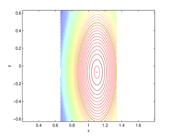
Figure 1: Equilibrium for the initial conditions given in the text of section 2. The bounding surface, shown in green, corresponds to $u_{b}=5.5\ Wb$ while at the magnetic axis, which is located at $(x_{a},y_{a})=(1.1,-0.07)$, $u_{a}=7.8\ Wb$.

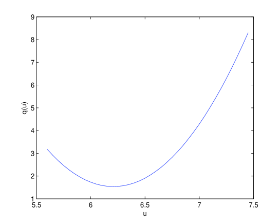
Figure 2: The safety factor for the equilibrium of Fig. 1 presenting a strong negative magnetic shear region. The outer bounding surface corresponds to $u=u_{b}=5.5\ Wb$ while at the magnetic axis $u=u_{a}=7.5\ Wb$

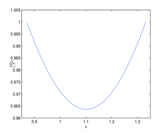
Figure 3: The axial magnetic field $B_{z}$, for equilibrium of Fig. 1 normalized to its center value of $B_{z0}=3.2\ T$.

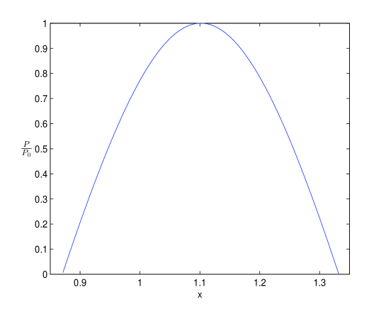
Figure 4: The pressure for equilibrium of Fig. 1 normalized to its center value of $P_{0}=2.1046\times 10^{5}Pa$.

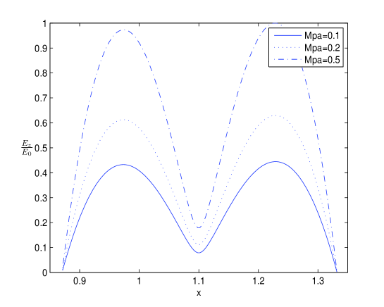
Figure 5: The electric field $E_{z}$, for equilibrium of Fig. 1 normalized to its maximum value of $E_{0}=5.4851\;kV\;m^{-1}$.

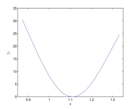
Figure 6: The axial current density at the midpalne $A(x,y=0)$ for the equilibrium of Fig. 1. It is hollow in connection with the negative magnetic shear of Fig. 2.

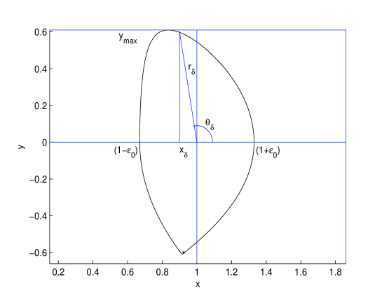
Figure 7: Bounding flux surface for the asymmetric case defined by Eqs. (4-4), possesing a divertor, null X-point at $P_{X}(x_{X},y_{X})=(0.9139,-0.6105)$.

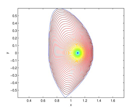
Figure 8: The numerical solution of Eq. (7) for the parameter values given in the text of section 4.

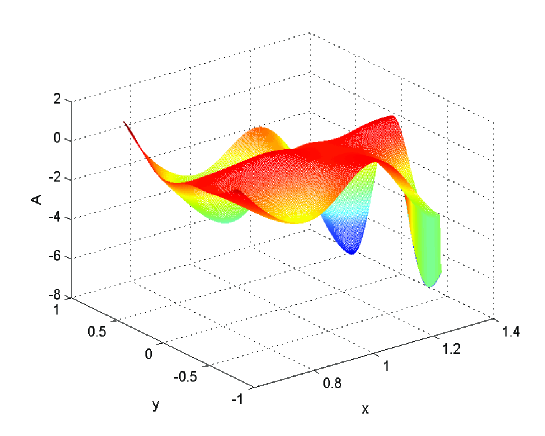
Figure 9: The stability function $A$ for the equilibrium of Fig. 1. At the upper part $(y>0)$ of the equilibrium it mostly assumes positive values, while at the lower part $(y<0)$ it assumes negative values.

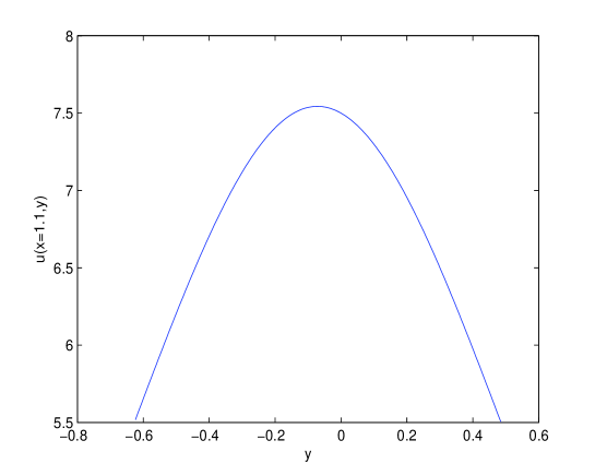
Figure 10: The poloidal magnetic flux function $u(x=1.1,y)$ for the equilibrium of Fig. 1. It is slightly up-down asymmetric with repsect to $y=0$.

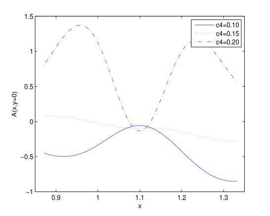
Figure 11: The stability function at the midpalne $A(x,y=0)$ for the equilibrium of Fig. 1, for various values of the nonlinear constant $c_{4}$. It appears that nonlinearity acts in favour of the stability.

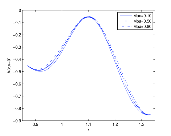
Figure 12: The stability function at the midplane $A(x,y=0)$ for the equilibrium of Fig. 1, for various values of the flow parameter $M_{pa}$. It appears that flow acts in favour of the stability, though in a weak manner.

4 Numerical asymmetric equilibrium with X-point

We consider now the direct numerical solution of Eq. (7) with a prescribed boundary possessing a divertor null X-point. We first will specify the boundary. The boundary conditions for the flux function $u$ is $u_{b}=1\ Wb$ on the prescribed boundary curve and $u_{a}=0\ Wb$ on the magnetic axis. The magnetic axis is taken to be Shafranov shifted at $x_{a}=1+x_{s}=1.1$. The model thus has three free parameters which are the Shafranov shift $x_{s}$, the elongation $\kappa$ and the triangularity $\delta.$ Their values are taken as $x_{s}=0.1$, $\kappa=1.86$ and $\delta=0.5$, in accordance with the corresponding data of the ITER project. The bounding flux surface, for the aymmetric case, is shown in Fig. 7. We take the values $a=2\ m$, $R_{0}=6.2\ m$ for the minor and major radius of the “torus” respectively for which the inverse aspect ratio is $\epsilon_{0}=0.32$.

The equation for the upper part of the bounding flux surface, which if taken to hold for the lower part as well would give a symmetric bounding surface, is

$$x_{b} = 1+\epsilon_{0}cos(\tau+\alpha sin(\tau))$$

$$y_{b} = y_{max}sin(\tau)$$ (18)

where $y_{max}=\kappa\epsilon_{0}$ with $\delta=(1-x_{\delta})/\epsilon_{0}$, and $\alpha=sin^{-1}(\delta)$. Thus the following relations hold: $x_{\delta}=1-\delta\epsilon_{0}$ and $\theta_{\delta}=\pi-tan^{-1}(\kappa/\delta)$. The parameter $\tau$ is any increasing function of the polar angle $\theta$, satisfying $\tau(0)=0$, $\tau(\pi)=\pi$ and $\tau(\theta_{\delta})=\pi/2$. In our model we take

$$\tau(\theta) = t_{0}\theta^{2}+t_{1}\theta^{n}$$

$$t_{0} = \frac{\theta_{\delta}^{n}-\frac{1}{2}\pi^{n}}{\pi\theta_{\delta}^{n}-\theta_{\delta}^{2}\pi^{n-1}}$$

$$t_{1} = \frac{-\theta_{\delta}^{2}+\frac{1}{2}\pi^{2}}{\pi\theta_{\delta}^{n}-\theta_{\delta}^{2}\pi^{n-1}}$$ (19)

with $n=8$. In order to complete the asymmetric bounding curve we specify now the lower part of it $(y<0)$ as follows. The left lower branch of the curve is given by

$$x_{b} = 1+\epsilon_{0}cos(\theta)$$

$$y_{b} = -[2p_{1}\epsilon_{0}(1+cos\theta)]^{1/2}$$

$$p_{1} = \frac{y_{max}^{2}}{2\epsilon_{0}(1+cos\theta_{\delta})},\;\;\;\;(\pi\leq\theta\leq 2\pi-\theta_{\delta})$$ (20)

while the right lower branch of the curve is given by

$$x_{b} = 1+\epsilon_{0}cos(\theta)$$

$$y_{b} = -[2p_{2}\epsilon_{0}(1-cos\theta)]^{1/2}$$

$$p_{2} = \frac{y_{max}^{2}}{2\epsilon_{0}(1-cos\theta_{\delta})},\;\;\;\;(2\pi-\theta_{\delta}\leq\theta\leq 2\pi)$$ (21)

The divertor null X-point is located at $x_{X}=1+\epsilon_{0}cos\theta_{\delta}=0.9139$ and $y_{X}=-y_{max}=-0.6105$.

The Laplacian operator $u_{xx}+u_{yy}$ is discretized on a rectangular grid where we have
$(1-\epsilon_{0})\leq x\leq(1+\epsilon_{0})$ and $-y_{max}\leq y\leq y_{max}$ with grid step $h$. The nine point formula is then employed [33]

$$\nabla^{2}u_{i,j} = \frac{1}{6h^{2}}\left[u_{i+1,j+1}+4u_{i+1,j}+u_{i+1,j-1}+4u_{i,j+1}+4u_{i,j-1}+u_{i-1,j+1}+\right.$$ (22)

$$\left.+4u_{i-1,j}+u_{i-1,j-1}-20u_{i,j}\right]$$

and when substituted into Eq. (7), the latter is written as $u_{i,j}^{(new)}=G(u)_{i,j}^{(old)}$ and is solved iteratively. The last term of Eq. (22) is taken to be the $u_{i,j}^{(new)}$ and the iterations stop (i.e. reaching convergence to the solution) when $|u_{i,j}^{(new)}-u_{i,j}^{(old)}|<0.001$. We stress again that the conditions $u_{b}=1$ on the boundary and $u_{{a}}=0$ on axis are imposed in every iteration. For $h=0.02$, and for the following values of the constants of Eq. (7), $c_{1}=-10.0,\;c_{2}=2.0,\;c_{3}=1.1,c_{4}=1.1$, a number of $N=165$ iterations were needed to obtain the desired accuracy. The solution is shown in Fig. 8. Although it seems that the solution is dependent on the specific value of the $h$ chosen, from the discrete two-dimensional matrix of $u_{i,j}$ produced, a two-dimensional Lagrange fitting is performed that yields a polynomial in $(x,y)$. This is h-independent. It is noted that the ripples of the flux function, appearing near the boundary of the equilibrium are due to numerical instabilities that are inevitable present in the calculation.

5 A stability consideration

We now address the important issue of the stability of the solutions constructed with respect to small linear MHD perturbations by means of the sufficient condition of [29]. This condition concerning internal modes states that a general steady state of a plasma of constant density and incompressible flow parallel to $\bf B$ is linearly stable to small three-dimensional perturbations if the flow is sub-Alfvénic ($M_{p}^{2}<1$) and $A\geq 0$, where $A$ is given below by (23). Consequently, using henceforth dimensionless quantities we set $\rho=1$. Also, for parallel flows (${\bf v}=M{\bf B}$) it holds $M_{p}\equiv M_{z}\equiv M$. In fact if the density is uniform at equilibrium it remains so at the perturbed state because of incompressibility. In the $u$-space for axisymmetric equilibria $A$ assumes the form

$$A = -{\bar{g}}^{2}\left[\frac{}{}({\bf j}\times\nabla u)\cdot({\bf B}\cdot\nabla)\nabla u+\right.$$ (23)

$$+ \left(\frac{M_{p}^{2}}{2}\right)^{{}^{\prime}}\frac{|\nabla u|^{2}}{(1-M_{p}^{2})^{3/2}}\left\{\frac{}{}\nabla u\cdot\nabla(B^{2}/2)+\right.$$

$$+ \left.\left.{\bar{g}}\frac{|\nabla u|^{2}}{(1-M_{p}^{2})^{1/2}}\frac{}{}\right\}\right]$$

with

$$\bar{g}:=\frac{P_{s}^{{}^{\prime}}(u)-(M_{p}^{2})^{{}^{\prime}}B^{2}/2}{1-M_{p}^{2}}$$

This condition, although complicated is accurate (a proof is provided in [29]) and all the computations and conclusions have been performed with great care. Specifically, its application to the equilibria constructed in sections 3 and 4 led to the following results:

1. Even a weak up-down asymmetry affects stability as indicated in Fig. 9 where we have checked thoroughly the values of the function $A$ for the equilibrium of Fig. 1. It turns out that at most of the upper part of the equilibrium, where $y>0$, $A$ assumes small positive values, while for the lower part of the equilibrium, $(y<0)$, it assumes small negative values. This slight $A$-up-down asymmetry is connected to the respective slight asymmetry of the flux function $u$ with respect to the vertical position $y$; the latter can be seen in Fig. 10 where the profile $u(x,y)$ is given at the point $x=1+x_{s}=1.1$. Though $A<0$ does not necessarily imply an unstable equilibrium because the condition is sufficient, the above result is consistent with the fact that up-down asymmetry may make the plasma unstable. For external modes this might relate to the vertical instability, e.g. [34].

2. The non linearity favours the stability as it is shown in Fig. 11 where $A$ is plotted as a function of $x$ at the midplane $y=0$ for increasing values of the non-linearity constant $c_{4}$.

3. The flow has a slight stabilizing effect. An example is given in Fig. 12 in connection with the flow parameter $M_{pa}$.

6 Summary

We have constructed and studied nonlinear translational symmetric equilibria with strong reversed magnetic shear and sheared incompressible flow non parallel to the magnetic field on the basis of a generalized Grad-Shafranov equation (Eq. (1)). This equation can be transformed to one identical in form with the static Grad-Shafranov equation which we have solved in a couple of alternative ways: i) by using an ansatz for the unknown magnetic flux function (Eq. (8) which reduces the original equation to a set of ODEs and algebraic constraints (Eqs. (10-15)); then this set of equations is solved numerically, and ii) fully numerically by prescribing anallyticaly a diverted boundary (Eqs. (4-4)). The equilibria constructed are typically dimagnetic (Fig. 3), have peacked pressure profiles (Fig. 4), hollow toroidal current densities (Fig. 6) and electric fields possessing a maximum (Fig. 5). The maximum of ${\bf E}$ takes larger values as the flow amplitude increases but its position is insensitive to the flow.

For parallel flows application of a condition for linear stability implies that the equilibrium nonlinearity has a stabilizing effect together with a weaker stabilizing impact of the sheared flow in agreement with past nonlinear equilibrium studies [17, 18, 19]. Also even a small up-down asymmetry influences stability.

Finally it would be interesting to try constructing equilibria with flow and reversed current density in connection with non nested magnetic surfaces thus generalizing the static ones of [21, 22, 24] and extend the study to axially symmetric equilibria by possibly generalizing the ansatz (8) in order to examining the impact of toroidicity.

Appendix: Quantities appearing in the ODEs and algebraic constraints (11-15)

The functions $G_{1},\;G_{4},\;G_{5}$ appearing into Eqs. (11), (12), (13) are given by

$$G_{1} = -4D_{0}D_{1}(N_{2}-f)+4D_{1}^{2}(N_{1}-fD_{1})-6D_{0}(N_{1}-fD-{1})$$ (24)

$$- 2D_{0}D_{0}^{{}^{\prime}}(N_{1}^{{}^{\prime}}-fD_{1}^{{}^{\prime}}-f^{{}^{\prime}}D_{1})+2(D_{0}^{{}^{\prime}})^{2}(N_{1}-fD_{1})-2D_{0}^{2}D_{1}^{{}^{\prime}}f^{{}^{\prime}}+$$

$$+ c_{1}D_{0}^{2}D_{1}+c_{2}D_{0}^{2}N_{1}-c_{3}f^{2}D_{0}^{2}D_{1}+2c_{3}fD_{0}^{2}N1+$$

$$+ 3c_{4}f^{2}D_{0}^{2}N_{1}-2c_{4}f^{3}D_{0}^{2}D_{1}$$

$$G_{4} = -2(N_{2}-f)+\frac{2D_{1}(N_{1}-fD_{1})}{D_{0}}-2D_{0}^{{}^{\prime}}(N_{2}^{{}^{\prime}}-f^{{}^{\prime}})-$$ (25)

$$- 2D_{1}^{{}^{\prime}}(N_{1}^{{}^{\prime}}+D_{1}N_{2}^{{}^{\prime}}-N_{2}D_{1}^{{}^{\prime}})+2c_{1}D_{1}^{2}+2c_{2}N_{1}D_{1}+c_{3}N_{1}^{2}+$$

$$+ 2c_{3}fD_{0}N_{2}+2c_{3}N_{1}N_{2}D_{1}-c_{3}f^{2}D_{0}-c_{3}N_{2}^{2}D_{1}^{2}-c_{3}D_{0}N_{2}^{2}-$$

$$- c_{4}f^{3}D_{0}-c_{4}N_{2}^{3}D_{1}^{2}+3c_{4}fD_{0}N_{2}^{2}+3c_{4}N_{2}N_{1}^{2}-2c_{4}N_{2}^{3}D_{0}$$

$$G_{5} = -2D_{1}^{{}^{\prime}}N_{2}^{{}^{\prime}}+c_{1}D_{1}+c_{2}N_{1}+2c_{3}N_{1}N_{2}-c_{3}N_{2}^{2}D_{1}-2c_{4}N_{2}^{3}D_{1}+$$ (26)

$$+ 3c_{4}N_{1}N_{2}^{2}$$

The functions $G_{2},\;G_{3}$ appearing into Eqs. (14-15) are given by

$$G_{2} = -2D_{1}^{2}(N_{2}-f)+\frac{2D_{1}^{3}(N_{1}-fD_{1})}{D_{0}}+2c_{1}D_{0}D_{1}^{2}-c_{3}f^{2}D_{0}D_{1}^{2}-$$ (27)

$$- c_{4}f^{3}D_{0}D_{1}^{2}-10D_{0}(N_{2}-f)+4D_{1}(N_{1}-fD_{1})-c_{3}f^{2}D_{0}^{2}-$$

$$- 2c_{4}f^{3}D_{0}^{2}+2f^{{}^{\prime}}D_{0}^{{}^{\prime}}(D_{1}^{2}+2D_{0})-2D_{0}^{{}^{\prime}}(f^{{}^{\prime}}D_{0}+fD_{0}^{{}^{\prime}})$$

$$- 2D_{1}D_{1}^{{}^{\prime}}(f^{{}^{\prime}}D_{0}+fD_{0}^{{}^{\prime}})-c_{3}N_{2}^{2}D_{0}^{2}-c_{4}N_{2}^{3}D_{0}^{2}-2N_{1}^{{}^{\prime}}D_{0}^{{}^{\prime}}D_{1}-$$

$$- 2N_{1}^{{}^{\prime}}D_{0}D_{1}^{{}^{\prime}}-2N_{2}^{{}^{\prime}}D_{0}D_{0}^{{}^{\prime}}+2fD_{0}(D_{1}^{{}^{\prime}})^{2}+2N_{2}(D_{0}^{{}^{\prime}})^{2}+4N_{1}D_{0}^{{}^{\prime}}D_{1}^{{}^{\prime}}+$$

$$+ 2c_{2}N_{1}D_{0}D_{1}+2c_{3}fD_{0}D_{1}N_{1}+c_{3}N_{1}^{2}D_{0}+2c_{3}fD_{0}^{2}N_{2}+3c_{4}fD_{0}N_{1}^{2}+$$

$$+ 3c_{4}f^{2}D_{0}^{2}N_{2}$$

and

$$G_{3} = -4D_{1}(N_{2}-f)+\frac{4D_{1}^{2}(N_{1}-fD_{1})}{D_{0}}-2c_{3}f^{2}D_{0}D_{1}-2c_{4}f^{3}D_{0}D_{1}+$$ (28)

$$+ 4D_{1}f^{{}^{\prime}}D_{0}^{{}^{\prime}}-2c_{3}N_{2}^{2}D_{0}D_{1}-2c_{4}N_{2}^{3}D_{0}D_{1}-2(f^{{}^{\prime}}D_{0}+fD_{0}^{{}^{\prime}})D_{1}^{{}^{\prime}}-$$

$$- 2N_{1}^{{}^{\prime}}D_{0}^{{}^{\prime}}-2N_{1}^{{}^{\prime}}D_{1}D_{1}^{{}^{\prime}}-2N_{2}^{{}^{\prime}}D_{0}^{{}^{\prime}}D_{1}-2N_{2}^{{}^{\prime}}D_{0}D_{1}^{{}^{\prime}}+2N_{1}(D_{1}^{{}^{\prime}})^{2}+$$

$$+ 4N_{2}D_{0}^{{}^{\prime}}D_{1}^{{}^{\prime}}+2N_{1}-2N_{2}D_{1}+c_{1}D_{1}^{3}+2c_{1}D_{0}D_{1}+c_{2}N_{1}D_{1}^{2}+$$

$$+ 2c_{2}N_{1}D_{0}+2c_{3}fD_{0}N_{1}+c_{3}N_{1}^{2}D_{1}+2c_{3}fD_{0}D_{1}N_{2}+$$

$$+ +2c_{3}N_{1}N_{2}D_{0}+c_{4}N_{1}^{3}+6c_{4}N_{1}N_{2}fD_{0}$$

Aknowledgments

One of the authors (GNT) would like to thank Henri Tasso and George Poulipoulis for useful discussions.

The work leading to this article was performed within the participation of the University of Ioannina in the Association Euratom-Hellenic Republic, which is supported in part by the European Union (Contract of Association No. ERB 5005 CT 99 0100) and by the General Secretariat of Research and Technology of Greece. The views and opinions expressed herein do not necessarily reflect those of the European Commission.

References

References

- [1] E. K. Mashke and H. Perrin Phys. Lett. A 102, 106 (1984).
- [2] R. A. Clemente and R. Farengo, Phys. Fluids 27, 776 (1984).
- [3] J. M. Greene, Plasma Phys. Controlled Fusion 30, 327 (1988).
- [4] G. N. Throumoulopoulos and H. Tasso, Phys. Plasmas 4, 1492 (1997).
- [5] J. P. Goedbloed and A. Lifschitz, Phys. Plasmas 4, 3544 (1997).
- [6] H. Tasso and G. N. Throumoulopoulos, Phys. Plasmas 5, 2378 (1998).
- [7] Ch. Simintzis, G. N. Throumoulopoulos G. Pantis and H. Tasso, Phys. Plasmas 8, 2641 (2001).
- [8] V. I. Ilgisonis and Yu. I. Pozdnyakov, Plasma Phys. Reports 28, 83 (2002).
- [9] G. N. Throumoulopoulos, H. Weitzner and H. Tasso, Phys. Plasmas 13, 122501 (2006).
- [10] D. Apostolaki, G. N. Throumoulopoulos and H. Tasso, 35th EPS Conference on Plasma Phys. Hersonissos, 9-13 June 2008, ECA Vol. 32, P-2.057 (2008).
- [11] A. H. Khater and S. M. Moawad, Phys. Plasmas 16, 122506 (2009).
- [12] Ap Kuiroukidis, Plasma Phys. Control. Fusion 52, 015002 (2010).
- [13] K. H. Tsui, C. E. Navia, A. Serbeto and H. Shigueoka, Phys. Plasmas 18, 072502 (2011).
- [14] B. Shi, Nucl. Fusion 51, 023004 (2011).
- [15] G. N. Throumoulopoulos, H. Tasso, Phys. Plasmas 19, 014504 (2012).
- [16] Ap Kuiroukidis and G. N. Throumoulopoulos, Phys. Plasmas 19, 022508 (2012).
- [17] G. N. Throumoulopoulos, H. Tasso and G. Poulipoulis, J. Phys. A: Math. Theor. 42, 335501 (2009).
- [18] G. N. Throumoulopoulos. and H. Tasso Phys. Plasmas 17, 032508 (2010).
- [19] Ap Kuiroukidis and G. N. Throumoulopoulos, Nonlinear translational symmetric equilibria relevant to the L-H transition, J. Plasma Physics, Available on CJO 2012 doi:10.1017/S0022377812000918.
- [20] P. M. Bellan, Phys. Plasmas 9, 3050 (2002).
- [21] A. A. Martynov, S. Yu. Medvedev, L. Vilard, PRL 91, 085004 (2003).
- [22] S. Wang, PRL 93, 155007 (2004).
- [23] E. Strumberger, S. Günter, J. Hobrik, V. Igochine et al., Nucl. Fusion 44,464 (2004).
- [24] P. Rodrigues and J. P. S. Bizzaro, PRL 99, 125001 (2007).
- [25] P.-A. Gourdain and J.-N. Leboeuf, Phys. Plasmas 16, 112506 (2009).
- [26] C. G. L. Martins, M. Roberto, I. L. Caldas, and F. L. Braga, Phys. Plasmas 18, 082508 (2011).
- [27] S. Friedlander, M. M. Vishik, Chaos 5, 416 (1995).
- [28] V. A. Vladimirov and K. I. Ilin, Phys. Plasmas 5, 4199 (1998).
- [29] G. N. Throumoulopoulos and H. Tasso, Phys. Plasmas 14, 122104 (2007).
- [30] P. C. de Vries, E. Joffrin, M. Brix, C. D. Challis et al., Nucl. Fusion 49, 075007 (2009).
- [31] M. W. Shafer, G. R. McKee, M. E. Austin, K. H. Burrell et. al., PRL 103, 075004 (2009).
- [32] J. Wesson Tokamaks, Fourth Edition, Oxford Engineering Science Series 149, Oxford (2011).
- [33] C. Gerald and P. Wheatley Applied Numerical Analysis, Addison-Wesley (1989).
- [34] R. Fitzpatrick, Nucl. Fusion 51, 053007 (2011).