Full halo coronal mass ejections: Do we need to correct the projection effect in terms of velocity?
Abstract
The projection effect is one of the biggest obstacles in learning the real properties of coronal mass ejections (CMEs) and forecasting their geoeffectiveness. To evaluate the projection effect, 86 full halo CMEs (FHCMEs) listed in the CDAW CME catalog from 2007 March 1 to 2012 May 31 are investigated. By applying the Graduated Cylindrical Shell (GCS) model, we obtain the de-projected values of the propagation velocity, direction and angular width of these FHCMEs, and compare them with the projected values measured in the plane-of-sky. Although these CMEs look full halo in the view angle of SOHO, it is found that their propagation directions and angular widths could vary in a large range, implying projection effect is a major reason causing a CME being halo, but not the only one. Furthermore, the comparison of the de-projected and projected velocities reveals that most FHCMEs originating within 45∘ of the Sun-Earth line with a projected speed slower than 900 km s-1 suffer from large projection effect, while the FHCMEs originating far from the vicinity of solar disk center or moving faster than 900 km s-1 have small projection effect. The results suggest that not all of FHCMEs need to correct projection effect for their velocities.
1 Introduction
Halo coronal mass ejections (CMEs), which appear to surround the occulting disk of coronagraphs, were first reported by Howard et al. (1982) based on observations from Solwind on P78-1. Since then, the properties and geoeffectiveness of halo CMEs have been widely studied and discussed (e. g. Cyr et al., 2000; Wang et al., 2002; Yashiro et al., 2004; Burkepile et al., 2004; Schwenn et al., 2005; Lara et al., 2006; Gopalswamy, 2009; Gopalswamy et al., 2007, 2010b; Temmer et al., 2008; Wang et al., 2011; Cid et al., 2012, and reference therein).
Most aforementioned studies were based on the analyses of the observations from single-point observations, such as Solar Maximum Mission (SMM), Solar & Heliospheric Observatory (SOHO), etc. However, the projection effect, unavoidable in single-point observations, would significantly distort the real geometric and kinematic parameters of CMEs, especially for full halo CMEs (FHCMEs) which are thought to originate from the vicinity of the solar disk center (e. g. Howard et al., 1985; Hundhausen, 1993; Webb and Howard, 1994; Sheeley et al., 1999; Vršnak et al., 2007; Howard et al., 2008; Gao et al., 2009; Temmer et al., 2009; Wang et al., 2011). Various models, such as cone models (e. g. Zhao et al., 2002; Xie et al., 2004; Xue et al., 2005; Michalek, 2006; Zhao, 2008), and some simple de-projection models (e.g. Shen et al., 2007; Howard et al., 2007, 2008) have been developed to get the real parameters of CMEs. Based on a de-projection method, for example, Howard et al. (2008) discussed the projection effect on the kinematic properties of CMEs. They found that the magnitude of corrected measurements of CMEs can differ significantly from the projected measurements , and the angular widths of CMEs are correlated with their speeds.
The successful launch of the Solar TErrestrial RElations Observatory (STEREO) (Kaiser et al., 2008) first provided multiple-point observations of CMEs. Based on different assumptions, various models, such as Graduated Cylindrial Shell (GCS) model(Thernisien et al., 2006, 2009; Thernisien, 2011), triangulation methods(e.g. Temmer et al., 2009; Lugaz et al., 2009, 2010; Liu et al., 2010; Lugaz, 2010; Liu et al., 2012), mask fitting methods(Feng et al., 2012, 2013), Geometric Localisation (GL)(Koning et al., 2009), and Local Correlation Tracking Plus Triangulation (LCT-TR) (Mierla et al., 2009) were developed. The accuracy and the difference of some models have been compared and discussed by Lugaz (2010) and Feng et al. (2013). Since then, the geometric and kinematic parameters of CMEs could be determined in a more reliable way.
Since STEREO will not always be there, however, space weather forecasting still relies on single-point observations, from which projected values are measured. Thus, it is time to re-evaluate how significantly the projection effect influences the CMEs’ parameters. Here we are particularly interested in the projection effect in terms of velocity, which is the most important parameters in space weather forecasting. FHCMEs, the most likely Earth-directed ones, are selected for this study. The CDAW CME catalog (Yashiro et al., 2004) is used to select events, and the time period is from 2007 March 1 to 2012 May 31, during which STEREO and SOHO observations are all available, and the separation angle between the twin spacecraft of STEREO varied from 1∘ to 233∘. It results in a sample of 86 FHCMEs. In section 2, we will briefly introduce the GCS model and its application on the FHCMEs. The de-projected properties of FHCMEs will be presented in Section 3. In the Section 4, we will show the significance of the projection effect and try to answer the question which kind of FHCMEs need correction. A summary and conclusions are given in the last section.
2 Method
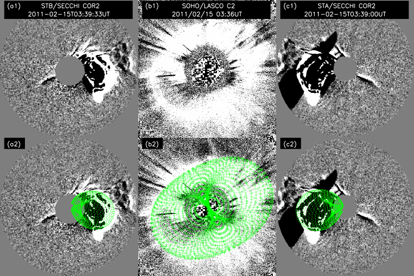
GCS model is an empirical and forward fitting method to represent the structure of flux rope-like CMEs (Thernisien et al., 2006, 2009; Thernisien, 2011), and has proved to be one of the best models to derive real parameters from projected images (e.g., Liu et al., 2010; Poomvises et al., 2010; Vourlidas et al., 2011; Shen et al., 2012, 2013). The GCS model has six free geometric parameters, which are the propagation longitude and latitude , aspect ratio , tilt angle with respect to the equator, the half-angle between the legs, and finally, the height of the CME leading edge (see Fig. 1 of Thernisien et al. (2006)). To derive the de-projected parameters of CME, we adjust these six parameters manually to get the best match between the modeled CME and the observed CME in all STEREO and SOHO coronagraphs, i.e., STEREO/COR2 A and B and SOHO/LASCO. In this procedure, the contrast of images is carefully adjusted to distinguish the main body of CMEs and the associated shock fronts. The STEREO/SECCHI COR1 data is not used due to its poor quality.
Figure 1 shows an example of the GCS model’s fitting result. We find that there are 80% (69 out of 86) FHCMEs could be well fitted by the GCS model. For a well-fitted CME, a time series of its direction, angular width and height could be obtained. The CME real speed, , is derived by the linear fitting of the height-time points. To get a more reliable result, we calculate only for the CMEs recorded in at least 3 frames. In our sample, there are three CMEs, which appeared in only one or two frames, and therefor no speed can be calculated for them. Table 1 shows the numbers of CMEs in different groups.
| Group I | Group II | Group III | Total |
|---|---|---|---|
| 66 (59) | 3 | 17 | 86 |
Note: Group I: CME is well fitted by GCS model and linear fitting speed could be obtained. The number in the parentheses is the number of CMEs in which the could not be calculated.. Group II: CME is well fitted by GCS model, but no speed is available. Group III: CME cannot be fitted by GCS model.
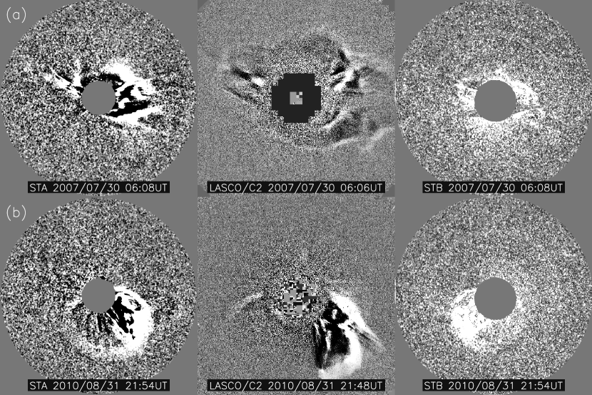
Why cannot the 17 CMEs in group III be fitted by the GCS model? We find that there are two reasons: First, the CME pattern is contaminated by other transient structures, which makes the boundary of the CME unclear. Such a phenomenon could be found in 12 events. As an example, the upper panels of Figure 2 show the 2007 July 30 event. At 06:06 UT, there are probably three CMEs recorded by coronagraphs simultenously. Secondly, the CME is away from a flux rope-like shape. The other 5 events are in this case. The lower panels of Figure 2 show an example, which occurred on 2010 August 31. One can see that one part of the CME is much brighter than other part, especially in the SOHO image. Such a phenomenon is probably due to the presence of ambient streamers or other pre-existing CMEs/shocks. Thus it cannot be the evidence that the CME is not a flux rope-like structure.
An online list is compiled to show the de-projected parameters of these FHCMEs, which could be found at http://space.ustc.edu.cn/dreams/fhcmes/. This list is being continuously updated for new events, It should not be surprising if some most recent events in the online list are not in the sample of this study. In this list, the propagation direction (given by longitude and latitude), the deviation angle () between the direction and the Sun-Earth line, the face-on angular width (, which is , in which is the half-angle of the cone) and the velocity () derived from the GCS model are given. The projected speed, , is also given for comparison. It should be noted that is not simply adapted from the CDAW CME catalog, because the speed it provides is from the measurements of the CME main front in the C2 and C3 field of view (FOV), which is much larger than STEREO COR2’s FOV where is derived. Thus, to make a reasonable comparison between the projected and de-projected speed, we re-calculate the projected speed by fitting the height-time measurements provided by the CDAW CME catalog in the FOV of COR2. Note, there are 7 events having no due to data points less than 3.
It should be noted that we only studied the kinematic parameters of the CMEs during their propagation in the field of view of STEREO/COR2. The COR2 instrument observed the corona from 2 to 15 . Previous results indicated that the acceleration (deceleration)(Zhang and Dere, 2006) of CMEs mainly happened in the lower corona region. Thus, we use the constant speed assumption and the discussion about the real acceleration of these CMEs, similar as Howard et al. (2008) did, are ignored in this work. In addition, by examine the fitting results for the FHCME events we studied in this paper carefully, we found that almost all the de-projected height-time profiles could be well fitted by straight lines.
3 De-projected Properties of FHCMEs

Figure 3(a) shows the distribution of the deviation angle, , of FHCMEs. It could vary in the full range from about 0∘ to nearly 90∘ with an average angle of 35∘. Most of them, occupying a fraction of 86% (59 out of 69), are smaller than 50∘, and a few of them could be very large. It suggests that the projection effect is indeed the main reason for CMEs being halo, but not always. On the other hand, about 14% (10 out of 69) of FHCMEs are very wide with angular width . This could be also seen in Figure 3(b). Although the projected angular width of all the CMEs in SOHO/LASCO FOV are all 360∘, the real angular width of them varies in a wide range from as narrow as 44∘ to as wide as 193∘. The average value of the angular width is about 103∘, much larger than that of a normal CME, which is about 60∘ (Wang et al., 2011). It is found that 45% of FHCMEs are wider than 100∘. This fact does imply that FHCMEs consist of a significant number of fast and wide CMEs.
A wider CME tends to be faster. This phenomenon was revealed in previous works by, e.g., Gopalswamy et al. (2001), Yashiro et al. (2004), Burkepile et al. (2004), Vršnak et al. (2007) and Howard et al. (2008), and also could be seen in Figure 4, which shows the scatter plot between the angular width and . It is found that there is a weak but positive correlation. The correlation coefficient is 0.48. A similar correction was shown in Vršnak et al. (2007) as Figure 1(a), in which the projected plane-of-sky velocity and angular width of the non-halo CMEs are compared. Besides, the bottom panel of Figure 3 shows the distribution of . The real speeds of these CMEs vary from 274 km s-1 to 2016 km s-1 with an average speed of 985 km s-1. The difference between the real speeds and projected speeds will be detailedly studied in the next section.

4 Projection Effect of FHCMEs

Projection effect undoubtedly exists for FHCMEs. In terms of space weather forecasting, two parameters, velocity and direction, are the most important. Direction is at secondary place for FHCMEs because most of them may encounter the Earth. The influence of the projection effect of the direction will be briefly discussed in the last section. Here we focus on the first priority parameter, the velocity.
First we define a parameter to measure the significance of the projection effect in velocity, which is . In principle, one could expect that should attain a value equal to or larger than unity. means there is no projection effect, while indicates the presence of projection effect. The larger the value of is, the more significant is the projection effect. Figure 5 shows the distribution of , which locates in a range from 0.78 to 2.21.
In this work, the uncertainty of the came from the errors of the GCS model’s heights and the linear fitting process. In Thernisien et al. (2009), they found that the mean uncertainties in the GCS model’s heights is about 0.48. By taken this uncertainty into the linear fitting process, we found that the mean relative error of the is about 12% for these events. It is worthy to note that the SOHO/LASCO observations in our study provide an additional constraint on the free parameters. Thus, we believe that the uncertainties of should be even smaller. For simplicity, a 10%-uncertainty is finally applied. The uncertainty of the comes from the error in measurements of height of CME’s leading edge. Assume the error is 0.2 (about 7-pixel uncertainty in SOHO/LASCO C3 images), the mean value of the relative error of the for these events is 10%. Thus, we use 10% as the uncertainty for both and for all the events in the statistical analysis. We may think that a value of roughly between 0.8 and 1.2 indicates there is no projection effect. It is found that there are 22 out of 59 events showing obvious projection effect. The velocities of these FHCMEs need the correction.
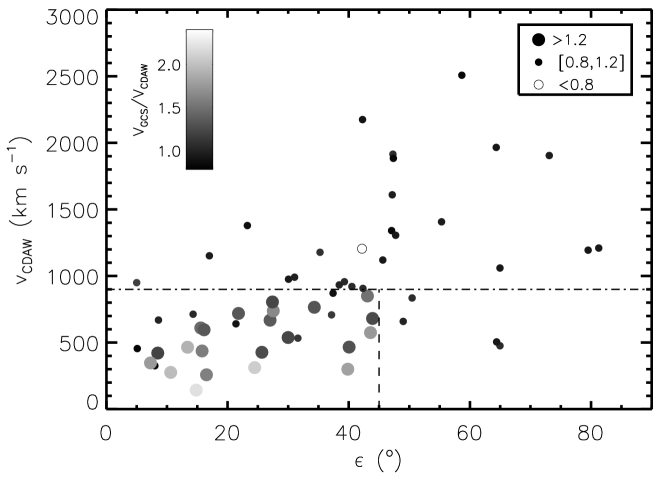
Why do some FHCMEs show significant projection effect and the others not? In order to answer the question, we investigate the dependence of on the deviation angle and the projected speed , which has been shown in Figure 6. Seen from this figure, a weak correlation between the projected speed and the deviation angle could be found. A similar correlation was shown in the Figure 2 of Vršnak et al. (2007), in which the location of the CME-related flare (treated as the source region of the CMEs) and the plane-of-sky speeds of these CMEs for non-halo CMEs were used. In Figure 6, large dots, small dots and open circles indicate the events with larger than 1.2, between 0.8 and 1.2, and smaller than 0.8, respectively. In addition, the gray scale of the symbols is used to indicate the value of . It can be seen readily that the events with a significant projection effect concentrate in the lower-left corner of the plot. For the events with larger than or larger than 900 km s-1, the values of are all close to unity, except one smaller than 0.8. Thus, we tentatively conclude that all the FFHCMEs which show obvious projection effect () are originating within 45∘ of the Sun-Earth line and moving slower than 900 km s-1 in the plane-of-sky. On the other hand, there are a total of 30 events in the region and km s-1, and 73% (22 out of 30) of these events have a large value of . These results clearly suggests that, although the projection effect reaches maximum for FHCMEs, not all of FHCMEs need to be corrected the effect in terms of velocity. If assuming CMEs propagate almost radially (though the fact is that CMEs may be deflected during propagation(e.g. Wang et al., 2004, 2006; Gopalswamy et al., 2010a; Gui et al., 2011; Shen et al., 2011; Zuccarello et al., 2012)), the angle approximately indicates the CME’s source location. Then we suggest that the projection effect of FHCMEs originating from the vicinity of solar disk center and not propagating too fast need be carefully checked.

The above analysis focuses on the relative difference between and . It should be noted that for a CME with larger than 1000 km s-1, 10% uncertainty will lead to an absolute difference larger than 200 km s-1 between them. This might cause a big error of about 10 hours in the CME transit time from the Sun to 1 AU. In such cases, the parameter might be questionable to show which CMEs have obvious projection effect. Thus, we further look into the absolute difference between the two velocities, which is . Figure 7 shows the distribution of . Here we assume a restrict and reasonable uncertainty of 100 km s-1. For a CME moving with speed of 1000 km s-1, this uncertainty leads to an acceptable uncertainty (about 4.6-hour) in the CME transit time from the Sun to 1 AU. It is found find that there are 26 out of 59 events with , 25 events with obviously larger than , and 8 events with obviously smaller than .
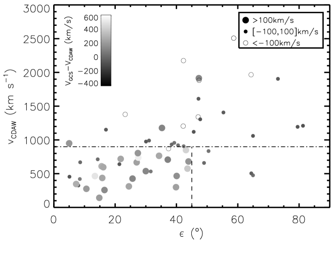
Similarly, the dependence of on and is shown in Figure 8. It could be seen that most (88% or 22 out of 25) events with km s-1 locate in the lower-left corner. If choosing the same thresholds like what we have done in Figure 6, i.e., and km s-1, we find that 73% (22 out of 30) of the events in the region have significant projection effect, and on the other hand, 90% (26 out of 29) of the events outside the region do not show obvious projection effect. These results are quite similar with those by using , and further confirm that the velocities of the FHCMEs originating from the vicinity of solar disk center and not propagating too fast are probably influenced by the projection effect.
For the events with , there are several reasons. First, the errors in the measurements and fitting procedures are large. Second, derived by fitting CME’s outline, while comes from the measurements of CME’s leading edge along a certain direction. The latter may probably be a shock rather than the CME body. We notice that all the CMEs with km s-1 are faster 850 km s-1 (particularly, 7 out of 8 CMEs are faster than 1200 km s-1). Such fast CMEs probably drive a shock and can be only recorded in a few frames by coronagraphs. Third, the overexpansion(e.g. MacQueen and Cole, 1985; Moore et al., 2007; Patsourakos et al., 2010) and the effect of aerodynamic drag(e.g. Chen, 1996; Cargill, 2004; Vršnak and Žic, 2007; Vršnak et al., 2008; Lugaz and Kintner, 2012; Vršnak et al., 2012) may another causes. Schwenn et al. (2005) found that the lateral expansion speed may larger than the radial speed with a factor of 1.2. In the projected image, it is hard to distinguish the expansion speed and the propagation speed of a CME. It is possible that the velocity determined in the projected observtaions might consist with expansion speed and the projected propagation speed. Thus, in some cases in which the expansion speeds are larger than their radial propagation speeds, their projected speeds might be larger than their real propagation speeds. In addition, the different values of the background solar wind speed at different latitudes might also caused the speed of some parts of CMEs faster than its real propagation velocity of its front due to solar wind drag. Thus, the apparent velocity which measured the fastest part of a CME on the plane-of-sky might faster than the real propagation velocity.
5 Summary and Conclusion
With the aids of GCS model, we investigate the de-projected parameters of the 69 FHCMEs from 2007 March 1 to 2012 May 31 based on the STEREO/COR2 and SOHO/LASCO observations. It is found that:
-
1.
A large fraction () of the FHCMEs could be fitted by the CGS model which assumes a flux-rope geometry of a CME. Those FHCMEs that cannot be well fitted are probably due the contamination/distortion by other structures. This result suggests that most CMEs are a flux-rope like structure. It consists with recent studies which argued that all (or large fraction of) CMEs are flux-rope structures based on remote or in-situ observations(e.g. Vourlidas et al., 2013; Xie et al., 2013; Yashiro et al., 2013; Zhang et al., 2013, and reference therein). Thus, models which treat the CME as a flux-rope(e.g. Chen, 1996; Hu et al., 2013; Hu and Dasgupta, 2006; Wang et al., 2009) are appropriate to study CMEs.
-
2.
Although the CMEs we chosen are all full halo CMEs in the view angle of SOHO, the de-projected angular width varies in a large range from 44∘ to 193∘. Moreover, about 30% of front-side FHCMEs have suggesting they are not Earth-directed. For those CMEs with large and small angular width, it is hard to expect that they would arrive at the Earth. Thus, if we simply use the front-side and full halo as criterion to determine Earth-directed CMEs, some wrong alerts will be made. In addition, the ratio that the Earth-direct CMEs arrival the Earth might be under-estimated if we simple use this criterion to determine the Earth-direct CME . However, some questions are still remained for these CMEs: (1) Whether all the these Earth-direct FHCMEs arrived at the Earth? (2) Can the ‘limb’ front-side FHCMEs arrive at the Earth? (3) Is there any criterion could be used to forecast whether a CME will arrive at the Earth? Such questions has been widely discussed based on projection parameters(e.g. Gopalswamy et al., 2007; Zhang et al., 2007). For the CME events studied in this work, their de-projected parameters have been well determined. Thus, these questions might be valuable to re-discussed.
-
3.
Not all the FHCMEs show obvious projection effect on the speed. Our results show that the FHCMEs originating within of the Sun-Earth line and moving with a projected speed slower than 900 km s-1 probably have obvious projection effect on the speed. Although the twin STEREO spacecraft allow us to get the de-projected parameters, they will not always be there and it is quite possible that CMEs can be only observed from one point. Thus, the criterion obtained above is particularly useful for us to determine whether or not a CME needs to correct projection effect, as the two parameters and applied in this criterion could be easily estimated from a single point observations. Why is the projection effect small for not on-disk () or fast () CMEs? A possible reason is that, these CMEs are usually wide enough to intersect with the plane of the sky. In this case, the measured velocity of the FHCMEs based on the projected coronagraph images may be close to their real propagation velocity because the fronts of CMEs are nearly circular.
Acknowledgements.
We acknowledge the use of CME catalog, the data from SECCHI instruments on STEREO and LASCO on SOHO. The CME catalog is generated and maintained at the CDAW Data Center by NASA and The Catholic University of America in cooperation with the Naval Research Laboratory. STEREO is the third mission in NASA Solar Terrestrial Probes program, and SOHO is a mission of international cooperation between ESA and NASA. We also acknowledge the NSSDC at Goddard Space Flight Center/NASA for providing Wind and ACE data. We benefited from discussions with X. P. Zhao. This work is supported by the Chinese Academy of Sciences (KZZD-EW-01), grants from the 973 key project 2011CB811403, NSFC 41131065, 41274173, 40874075, and 41121003, CAS the 100-talent program, KZCX2-YW-QN511 and startup fund, and MOEC 20113402110001 and the fundamental research funds for the central universities (WK2080000031).References
- Burkepile et al. (2004) Burkepile, J. T., A. J. Hundhausen, A. L. Stanger, O. C. St Cyr, and J. A. Seiden, Role of projection effects on solar coronal mass ejection properties: 1. A study of CMEs associated with limb activity, Journal of Geophysical Research, 109(A), 03,103, 2004.
- Cargill (2004) Cargill, P. J., On the Aerodynamic Drag Force Acting on Interplanetary Coronal Mass Ejections, Solar Physics, 221, 135, 2004.
- Chen (1996) Chen, J., Theory of prominence eruption and propagation: Interplanetary consequences, Journal of Geophysical Research, 101(A), 27,499–27,520, 1996.
- Cid et al. (2012) Cid, C., et al., Can a halo CME from the limb be geoeffective?, Journal of Geophysical Research, 117(A11), A11,102, 2012.
- Cyr et al. (2000) Cyr, O., et al., Properties of coronal mass ejections: SOHO LASCO observations from January 1996 to June 1998, Journal of Geophysical Research, 105(A8), 18,169–18,185, 2000.
- Feng et al. (2012) Feng, L., B. Inhester, Y. Wei, W. Q. Gan, T.-L. Zhang, and M. Y. Wang, Morphological Evolution of a Three-dimensional Coronal Mass Ejection Cloud Reconstructed from Three Viewpoints, Astrophysical Journal, 751(1), 18, 2012.
- Feng et al. (2013) Feng, L., B. Inhester, and M. Mierla, Comparisons of CME Morphological Characteristics Derived from Five 3D Reconstruction Methods, Solar Physics, 282(1), 221–238, 2013.
- Gao et al. (2009) Gao, P.-X., K.-J. Li, and Q.-X. Li, Kinetic properties of coronal mass ejections corrected for the projection effect in Cycle 23, Monthly Notices of the Royal Astronomical Society, 394(2), 1031–1036, 2009.
- Gopalswamy (2009) Gopalswamy, N., Halo coronal mass ejections and geomagnetic storms, Earth, 2009.
- Gopalswamy et al. (2001) Gopalswamy, N., S. Yashiro, M. L. Kaiser, R. A. Howard, and J.-L. Bougeret, Characteristics of coronal mass ejections associated with long-wavelength type II radio bursts, Journal of Geophysical Research, 106, 29,219, 2001.
- Gopalswamy et al. (2007) Gopalswamy, N., S. Yashiro, and S. Akiyama, Geoeffectiveness of halo coronal mass ejections, Journal of Geophysical Research, 112(A), 06,112, 2007.
- Gopalswamy et al. (2010a) Gopalswamy, N., P. Mäkelä, H. Xie, S. Akiyama, and S. Yashiro, Solar Sources of“Driverless”Interplanetary Shocks, TWELFTH INTERNATIONAL SOLAR WIND CONFERENCE. AIP Conference Proceedings, 1216, 452, 2010a.
- Gopalswamy et al. (2010b) Gopalswamy, N., S. Yashiro, H. Xie, S. Akiyama, and P. Mäkelä, Large Geomagnetic Storms Associated with Limb Halo Coronal Mass Ejections, Advances in Geosciences, 21, 71, 2010b.
- Gui et al. (2011) Gui, B., C. Shen, Y. Wang, P. Ye, and S. Wang, Quantitative Analysis of CME Deflections in the Corona, Solar Physics, 271, 111–139, 2011.
- Howard et al. (1982) Howard, R., D. Michels, N. SHEELEY, and M. Koomen, The Observation of a Coronal Transient Directed at Earth, Astrophysical Journal, 263(2), L101–&, 1982.
- Howard et al. (1985) Howard, R. A., N. R. J. Sheeley, D. J. Michels, and M. J. Koomen, Coronal mass ejections - 1979-1981, Journal of Geophysical Research, 90, 8173–8191, 1985.
- Howard et al. (2007) Howard, T. A., C. D. Fry, J. C. Johnston, and D. F. Webb, On the Evolution of Coronal Mass Ejections in the Interplanetary Medium, Astrophysical Journal, 667, 610, 2007.
- Howard et al. (2008) Howard, T. A., D. Nandy, and A. C. Koepke, Kinematic properties of solar coronal mass ejections: Correction for projection effects in spacecraft coronagraph measurements, Journal of Geophysical Research, 113(A1), A01,104, 2008.
- Hu and Dasgupta (2006) Hu, Q., and B. Dasgupta, A new approach to modeling non-force free coronal magnetic field, Geophysical Research Letters, 33(15), L15,106, 2006.
- Hu et al. (2013) Hu, Q., C. J. Farrugia, V. A. Osherovich, C. Möstl, A. Szabo, K. W. Ogilvie, and R. P. Lepping, Effect of Electron Pressure on the Grad–Shafranov Reconstruction of Interplanetary Coronal Mass Ejections, Solar Physics, 2013.
- Hundhausen (1993) Hundhausen, A. J., Sizes and Locations of Coronal Mass Ejections: SMM Observations from 1980 and 1984-1989, Journal of Geophysical Research, 98(A8), 13,177–13,200, 1993.
- Kaiser et al. (2008) Kaiser, M. L., T. A. Kucera, J. M. Davila, O. C. St Cyr, M. Guhathakurta, and E. Christian, The STEREO Mission: An Introduction, Space Science Reviews, 136(1), 5–16, 2008.
- Koning et al. (2009) Koning, C. A., V. J. Pizzo, and D. A. Biesecker, Geometric Localization of CMEs in 3D Space Using STEREO Beacon Data: First Results, Solar Physics, 256(1-2), 167–181, 2009.
- Lara et al. (2006) Lara, A., N. Gopalswamy, H. Xie, E. Mendoza-Torres, R. Pérez-Eríquez, and G. Michalek, Are halo coronal mass ejections special events?, Journal of Geophysical Research, 111(A), 06,107, 2006.
- Liu et al. (2010) Liu, Y., A. Thernisien, J. G. Luhmann, A. Vourlidas, J. A. Davies, R. P. Lin, and S. D. Bale, Reconstructing Coronal Mass Ejections with Coordinated Imaging and in Situ Observations: Global Structure, Kinematics, and Implications for Space Weather Forecasting, Astrophysical Journal, 722(2), 1762–1777, 2010.
- Liu et al. (2012) Liu, Y. D., et al., Interactions Between Coronal Mass Ejections Viewed in Coordinated Imaging and in Situ Observations, Astrophysical Journal Letters, 746(2), –, 2012.
- Lugaz (2010) Lugaz, N., Accuracy and Limitations of Fitting and Stereoscopic Methods to Determine the Direction of Coronal Mass Ejections from Heliospheric Imagers Observations, Solar Physics, 267(2), 411–429, 2010.
- Lugaz and Kintner (2012) Lugaz, N., and P. Kintner, Effect of Solar Wind Drag on the Determination of the Properties of Coronal Mass Ejections from Heliospheric Images, Solar Physics, 2012.
- Lugaz et al. (2009) Lugaz, N., A. Vourlidas, and I. I. Roussev, Deriving the radial distances of wide coronal mass ejections from elongation measurements in the heliosphere - application to CME-CME interaction, Annales Geophysicae, 27(9), 3479–3488, 2009.
- Lugaz et al. (2010) Lugaz, N., J. N. Hernandez-Charpak, I. I. Roussev, C. J. Davis, A. Vourlidas, and J. A. Davies, Determining the Azimuthal Properties of Coronal Mass Ejections from Multi-Spacecraft Remote-Sensing Observations with STEREO SECCHI, Astrophysical Journal, 715(1), 493–499, 2010.
- MacQueen and Cole (1985) MacQueen, R. M., and D. M. Cole, Broadening of Looplike Solar Coronal Transients, Astrophysical Journal, 299(1), 526–535, 1985.
- Michalek (2006) Michalek, G., An Asymmetric Cone Model for Halo Coronal Mass Ejections, Solar Physics, 237(1), 101–118, 2006.
- Mierla et al. (2009) Mierla, M., B. Inhester, C. Marqué, L. Rodriguez, S. Gissot, A. N. Zhukov, D. Berghmans, and J. Davila, On 3D Reconstruction of Coronal Mass Ejections: I. Method Description and Application to SECCHI-COR Data, Solar Physics, 259(1-2), 123–141, 2009.
- Moore et al. (2007) Moore, R. L., A. C. Sterling, and S. T. Suess, The width of a solar coronal mass ejection and the source of the driving magnetic explosion: A test of the standard scenario for CME production, Astrophysical Journal, 668(2), 1221–1231, 2007.
- Patsourakos et al. (2010) Patsourakos, S., A. Vourlidas, and G. Stenborg, The Genesis of an Impulsive Coronal Mass Ejection Observed at Ultra-high Cadence by AIA on SDO, The Astrophysical Journal Letters, 724(2), L188–L193, 2010.
- Poomvises et al. (2010) Poomvises, W., J. Zhang, and O. Olmedo, Coronal mass ejection propagation and expansion in three-dimensional space in the heliosphere based on stereo/secchi observations, The Astrophysical Journal Letters, 717, L159, 2010.
- Schwenn et al. (2005) Schwenn, R., A. Dal Lago, E. Huttunen, and W. D. Gonzalez, The association of coronal mass ejections with their effects near the Earth, Annales Geophysicae, 23(3), 1033–1059, 2005.
- Sheeley et al. (1999) Sheeley, N. R., J. H. Walters, Y. M. Wang, and R. A. Howard, Continuous tracking of coronal outflows: Two kinds of coronal mass ejections, Journal of Geophysical Research, 104(A), 24,739–24,768, 1999.
- Shen et al. (2007) Shen, C., Y. Wang, P. Ye, X. P. Zhao, B. Gui, and S. Wang, Strength of coronal mass ejection-driven shocks near the sun and their importance in predicting solar energetic particle events, Astrophysical Journal, 670(1), 849–856, 2007.
- Shen et al. (2011) Shen, C., Y. Wang, B. Gui, P. Ye, and S. Wang, Kinematic Evolution of a Slow CME in Corona Viewed by STEREO-B on 8 October 2007, Solar Physics, 269(2), 389–400, 2011.
- Shen et al. (2013) Shen, C., G. Li, X. Kong, J. Hu, X. D. Sun, L. Ding, Y. Chen, Y. Wang, and L. XIa, Compound Twin Coronal Mass Ejections in the 2012 May 17 GLE Event, Astrophysical Journal, 763(2), 114, 2013.
- Shen et al. (2012) Shen, C., et al., Super-elastic collision of large-scale magnetized plasmoids in the heliosphere, Nature Physics, 8(1), 923–928, 2012.
- Temmer et al. (2008) Temmer, M., A. M. Veronig, B. Vršnak, J. Rybák, P. Gömöry, S. Stoiser, and D. Maričić, Acceleration in Fast Halo CMEs and Synchronized Flare HXR Bursts, Astrophysical Journal, 673(1), L95–L98, 2008.
- Temmer et al. (2009) Temmer, M., S. Preiss, and A. M. Veronig, CME Projection Effects Studied with STEREO/COR and SOHO/LASCO, Solar Physics, 256(1-2), 183–199, 2009.
- Thernisien (2011) Thernisien, A., Implementation of the Graduated Cylindrical Shell Model for the Three-dimensional Reconstruction of Coronal Mass Ejections, The Astrophysical Journal Supplement Series, 194, 33, 2011.
- Thernisien et al. (2009) Thernisien, A., A. Vourlidas, and R. A. Howard, Forward Modeling of Coronal Mass Ejections Using STEREO/SECCHI Data, Solar Physics, 256(1), 111–130, 2009.
- Thernisien et al. (2006) Thernisien, A. F. R., R. A. Howard, and A. Vourlidas, Modeling of Flux Rope Coronal Mass Ejections, Astrophysical Journal, 652, 763, 2006.
- Vourlidas et al. (2011) Vourlidas, A., R. Colaninno, T. Nieves-Chinchilla, and G. Stenborg, The First Observation of a Rapidly Rotating Coronal Mass Ejection in the Middle Corona, Astrophysical Journal, 733(2), L23, 2011.
- Vourlidas et al. (2013) Vourlidas, A., B. J. Lynch, R. A. Howard, and Y. Li, How Many CMEs Have Flux Ropes? Deciphering the Signatures of Shocks, Flux Ropes, and Prominences in Coronagraph Observations of CMEs, Solar Physics, 284(1), 179–201, 2013.
- Vršnak and Žic (2007) Vršnak, B., and T. Žic, Transit times of interplanetary coronal mass ejections and the solar wind speed, Astronomy and Astrophysics, 472(3), 937–943, 2007.
- Vršnak et al. (2007) Vršnak, B., D. Sudar, D. Ruždjak, and T. Žic, Projection effects in coronal mass ejections, Astronomy and Astrophysics, 469(1), 339–346, 2007.
- Vršnak et al. (2008) Vršnak, B., D. Vrbanec, and J. Čalogović, Dynamics of coronal mass ejections. The mass-scaling of the aerodynamic drag, Astronomy and Astrophysics, 490(2), 811–815, 2008.
- Vršnak et al. (2012) Vršnak, B., et al., Propagation of Interplanetary Coronal Mass Ejections: The Drag-Based Model, Solar Physics, 285(1-2), 295–315, 2012.
- Wang et al. (2002) Wang, Y., P. Ye, S. Wang, G. Zhou, and J. Wang, A statistical study on the geoeffectiveness of Earth-directed coronal mass ejections from March 1997 to December 2000, Journal of Geophysical Research, 107(A11), 1340, 2002.
- Wang et al. (2004) Wang, Y., C. Shen, S. Wang, and P. Ye, Deflection of coronal mass ejection in the interplanetary medium, Solar Physics, 222, 329, 2004.
- Wang et al. (2006) Wang, Y., X. Xue, C. Shen, P. Ye, S. Wang, and J. Zhang, Impact of Major Coronal Mass Ejections on Geospace during 2005 September 7-13, Astrophysical Journal, 646, 625, 2006.
- Wang et al. (2009) Wang, Y., J. Zhang, and C. Shen, An analytical model probing the internal state of coronal mass ejections based on observations of their expansions and propagations, Journal of Geophysical Research, 114, –, 2009.
- Wang et al. (2011) Wang, Y., C. Chen, B. Gui, C. Shen, P. Ye, and S. Wang, Statistical study of coronal mass ejection source locations: Understanding CMEs viewed in coronagraphs, Journal of Geophysical Research, 116, –, 2011.
- Webb and Howard (1994) Webb, D. F., and R. A. Howard, The solar cycle variation of coronal mass ejections and the solar wind mass flux, Journal of Geophysical Research, 99, 4201–4220, 1994.
- Xie et al. (2004) Xie, H., L. Ofman, and G. Lawrence, Cone model for halo CMEs: Application to space weather forecasting, Journal of Geophysical Research, 109, A03,109, 2004.
- Xie et al. (2013) Xie, H., N. Gopalswamy, and O. C. St Cyr, Near-Sun Flux-Rope Structure of CMEs, Solar Physics, 284(1), 47–58, 2013.
- Xue et al. (2005) Xue, X. H., C. B. Wang, and X. K. Dou, An ice-cream cone model for coronal mass ejections, Journal of Geophysical Research, 110(A), 08,103, 2005.
- Yashiro et al. (2004) Yashiro, S., N. Gopalswamy, G. Michalek, O. C. St Cyr, S. P. Plunkett, N. B. Rich, and R. A. Howard, A catalog of white light coronal mass ejections observed by the SOHO spacecraft, Journal of Geophysical Research, 109(A), 07,105, 2004.
- Yashiro et al. (2013) Yashiro, S., N. Gopalswamy, P. Mäkelä, and S. Akiyama, Post-Eruption Arcades and Interplanetary Coronal Mass Ejections, Solar Physics, 284(1), 5–15, 2013.
- Zhang and Dere (2006) Zhang, J., and K. P. Dere, A Statistical Study of Main and Residual Accelerations of Coronal Mass Ejections, Astrophysical Journal, 649, 1100, 2006.
- Zhang et al. (2007) Zhang, J. and I. G. Richardson and D. F. Webb and N. Gopalswamy and E. Huttunen and J. C. Kasper and N. V. Nitta and W. Poomvises and B. J. Thompson and C. C. Wu and S. Yashiro and A. .N. Zhukov, Solar and interplanetary sources of major geomagnetic storms ( Dst −100 nT) during 1996 –- 2005, Journal of Geophysical Research, 112, 10102, 2007
- Zhang et al. (2013) Zhang, J., P. Hess, and W. Poomvises, A Comparative Study of Coronal Mass Ejections with and Without Magnetic Cloud Structure near the Earth: Are All Interplanetary CMEs Flux Ropes?, Solar Physics, 284(1), 89–104, 2013.
- Zhao (2008) Zhao, X. P., Inversion solutions of the elliptic cone model for disk frontside full halo coronal mass ejections, Journal of Geophysical Research, 113(A), 02,101, 2008.
- Zhao et al. (2002) Zhao, X. P., S. P. Plunkett, and W. Liu, Determination of geometrical and kinematical properties of halo coronal mass ejections using the cone model, Journal of Geophysical Research, 107(A), 1223, 2002.
- Zuccarello et al. (2012) Zuccarello, F. P., A. Bemporad, C. Jacobs, M. Mierla, S. Poedts, and F. Zuccarello, The Role of Streamers in the Deflection of Coronal Mass Ejections: Comparison between STEREO Three-dimensional Reconstructions and Numerical Simulations, Astrophysical Journal, 744(1), 66, 2012.