An accurate Newtonian description of particle motion around a Schwarzschild black hole

Abstract

A generalized Newtonian potential is derived from the geodesic motion of test particles in Schwarzschild spacetime. This potential reproduces several relativistic features with higher accuracy than commonly used pseudo-Newtonian approaches. The new potential reproduces the exact location of the marginally stable, marginally bound, and photon circular orbits, as well as the exact radial dependence of the binding energy and the angular momentum of these orbits. Moreover, it reproduces the orbital and epicyclic angular frequencies to better than $6\%$. In addition, the spatial projections of general trajectories coincide with their relativistic counterparts, while the time evolution of parabolic-like trajectories and the pericentre advance of elliptical-like trajectories are both reproduced exactly. We apply this approach to a standard thin accretion disc and find that the efficiency of energy extraction agrees to within $3\%$ with the exact relativistic value, while the energy flux per unit area as a function of radius is reproduced everywhere to better than $7\%$. As a further astrophysical application we implement the new approach within a smoothed particle hydrodynamics code and study the tidal disruption of a main sequence star by a supermassive black hole. The results obtained are in very good agreement with previous relativistic simulations of tidal disruptions in Schwarzschild spacetime. The equations of motion derived from this potential can be implemented easily within existing Newtonian hydrodynamics codes with hardly any additional computational effort.

1 Introduction

Our current understanding of some of the most energetic phenomena in the Universe (such as active galactic nuclei, X-ray binaries and gamma-ray bursts) involves the accretion of gas onto astrophysical black holes as the underlying mechanism for powering these sources (see e.g. Frank et al., 2002). It is clear that a satisfactory study of any of these systems should include a consistent treatment of the strong gravitational fields found in the vicinity of these relativistic objects. It is nonetheless remarkable that many of the early works on the subject, which were essentially Newtonian with a few general relativistic effects incorporated ‘by hand’, proved to be very successful at modelling a variety of accreting systems. For instance, the standard thin disc model of Shakura & Sunyaev (1973) is purely Newtonian and the only result from general relativity that it uses is the existence of the marginally stable circular orbit at which their disc model was truncated. Similarly, the model of a thick accretion disc introduced by Paczyńsky & Wiita (1980) (PW hereafter) is based on Newtonian dynamics with the substitution of the Newtonian gravitational potential $\Phi_{\text{\tiny$\mathrm{N}$ }}=-\mathrm{G}M/r$ by the pseudo-Newtonian potential

$$\Phi_{\text{\tiny$\mathrm{PW}$ }}(r)=-\frac{\mathrm{G}M}{r-2\,r_{\text{\tiny$\mathrm{g}$ }}},$$ (1.1)

where $r_{\text{\tiny$\mathrm{g}$ }}=\mathrm{G}M/\mathrm{c}^{2}$ is the so-called gravitational radius. The potential $\Phi_{\text{\tiny$\mathrm{PW}$ }}$ not only reproduces the correct location of the marginally stable and marginally bound circular orbits around a Schwarzschild black hole (at $r_{\text{\tiny$\mathrm{ms}$ }}=6\,r_{\text{\tiny$\mathrm{g}$ }}$ and $r_{\text{\tiny$\mathrm{mb}$ }}=4\,r_{\text{\tiny$\mathrm{g}$ }}$, respectively), but it also gives reasonable approximations to other quantities, e.g. binding energy (percentage error (p.e.) $\leqslant 13\%$) and angular momentum of circular orbits (p.e. $\leqslant 6\%$). Nevertheless, other quantities such as the orbital frequency $\Omega$ and the epicyclic frequency $\Omega^{\parallel}$ are not accurately reproduced (p.e. $\leqslant 50\%$ and $\leqslant 84\%$, respectively). This potential has been used in a large number of studies of accretion flows onto non-rotating black holes to mimic essential general relativistic effects within a Newtonian framework (e.g. Matsumoto et al., 1984; Abramowicz et al., 1988; Chakrabarti & Titarchuk, 1995; MacFadyen & Woosley, 1999; Hawley & Balbus, 2002; Lee & Ramírez-Ruiz, 2006; Rosswog et al., 2009).

Other pseudo-Newtonian potentials have been introduced to give better approximations to specific general relativistic features but at the price of reproducing some other properties with less accuracy. For instance, the pseudo-Newtonian potential introduced by Nowak & Wagoner (1991) (NW hereafter)

$$\Phi_{\text{\tiny$\mathrm{NW}$ }}(r)=-\frac{\mathrm{G}M}{r}\left(1-\frac{3\,r_{\text{\tiny$\mathrm{g}$ }}}{r}+\frac{12\,r^{2}_{\text{\tiny$\mathrm{g}$ }}}{r^{2}}\right),$$ (1.2)

reproduces the angular frequencies $\Omega$ and $\Omega^{\parallel}$ with better accuracy (p.e. $\leqslant 14\%$ and $\leqslant 42\%$, respectively) than $\Phi_{\text{\tiny$\mathrm{PW}$ }}$ while still giving the correct location of $r_{\text{\tiny$\mathrm{ms}$ }}$. However, it locates $r_{\text{\tiny$\mathrm{mb}$ }}$ at $\sim 3.5\,r_{\text{\tiny$\mathrm{g}$ }}$ and gives a less accurate estimate of the angular momentum of circular orbits (p.e. $\leqslant 30\%$). See Table 1 for a general comparison of the accuracy with which various relativistic properties are reproduced by $\Phi_{\text{\tiny$\mathrm{N}$ }}$, $\Phi_{\text{\tiny$\mathrm{PW}$ }}$, and $\Phi_{\text{\tiny$\mathrm{NW}$ }}$. Also see Artemova et al. (1996) for a comparison of the performance of $\Phi_{\text{\tiny$\mathrm{PW}$ }}$, $\Phi_{\text{\tiny$\mathrm{NW}$ }}$, and other pseudo-Newtonian potentials in reproducing the structure of a thin disc around rotating and non-rotating black holes.

Pseudo-Newtonian potentials have been widely used in accretion studies, although their range of applicability has been limited by the fact that no single one of them can reproduce equally well all of the various dynamical properties of Schwarzschild spacetime. For instance, a poor estimation of the orbital and epicyclic frequencies hampers their ability to capture time-dependent behaviour, such as the onset of instabilities in an accretion disc that might eventually lead to observed signatures (such as quasi-periodic oscillations; see e.g. Kato, 2001). On the other hand, a large error in the estimation of the binding energy of Keplerian circular orbits will lead to inaccurate estimates of the total luminosity of accretion discs. Another issue that is commonly overlooked is that most pseudo-Newtonian potentials are designed for accurately reproducing circular orbits but not necessarily more general trajectories. Nevertheless, they are frequently used in applications in which correctly reproducing general trajectories might be of crucial importance (e.g. the collapsing interior of a massive star towards a newborn black hole or successive passages of a star orbiting a black hole before becoming tidally disrupted).

In this work, we propose a generalization of the Newtonian potential that accurately describes the motion of test particles in Schwarzschild spacetime while still being formulated in entirely Newtonian language. In addition to the Newtonian $1/r$-term, our potential includes an explicit dependence on the velocity of the test particle. Following the nomenclature of Lagrangian mechanics (see e.g. Goldstein et al., 2002), we therefore call it a generalized Newtonian potential. Moreover, this potential is derived from the actual geodesic motion of test particles in Schwarzschild spacetime. This is in contrast to most pseudo-Newtonian potentials that are introduced as ad hoc recipes or as fitting formulae that mimic certain relativistic features (see, nevertheless, Abramowicz 2009 for an a posteriori derivation of $\Phi_{\text{\tiny$\mathrm{PW}$ }}$).

The remainder of the paper is organized as follows. In Section 2, the generalized potential and the corresponding equations of motion are derived and contrasted with the exact relativistic expressions. In Section 3, we compare the performance of our generalized potential with $\Phi_{\text{\tiny$\mathrm{N}$ }}$, $\Phi_{\text{\tiny$\mathrm{PW}$ }}$, and $\Phi_{\text{\tiny$\mathrm{NW}$ }}$ in reproducing several dynamical features of test particle motion in Schwarzschild spacetime including purely radial infall, Keplerian and non-Keplerian circular motion, general trajectories, pericentre advance, and two simple analytic accretion models (the thin disc model of Shakura & Sunyaev 1973 as generalized to Schwarzschild spacetime by Novikov & Thorne 1973 and the toy accretion model of Tejeda et al. 2012). At the end of this section we implement the new potential within a Newtonian smoothed particle hydrodynamics (SPH) code and simulate the tidal disruption of a solar-type star by a supermassive black hole. Finally, we summarize our results in Section 4.

2 Generalized Newtonian potential

Consider a test particle with four-velocity $u^{\text{\tiny$\mu$ }}=\mathrm{d}x^{\text{\tiny$\mu$ }}/\mathrm{d}\tau$ following a timelike geodesic in Schwarzschild spacetime (where $\tau$ is the proper time as measured by a comoving observer). Given the staticity and spherical symmetry of the Schwarzschild metric, the motion of the particle is restricted to a single plane (orbital plane) and is characterized by the existence of two first integrals of motion: its specific energy $\mathcal{E}$ and its specific angular momentum $h_{\text{\tiny$\mathrm{S}$ }}$ given by (e.g. Frolov & Novikov, 1998)

$$\mathcal{E}=-u_{t}=\mathrm{c}^{2}\left(1-\frac{2\,r_{\text{\tiny$\mathrm{g}$ }}}{r}\right)\,\frac{\mathrm{d}t}{\mathrm{d}\tau},$$ (2.1)

$$h_{\text{\tiny$\mathrm{S}$ }}=u_{\varphi}=r^{2}\frac{\mathrm{d}\varphi}{\mathrm{d}\tau},$$ (2.2)

where $\varphi$ is an angle measured within the orbital plane. These two equations together with the normalization condition of the four-velocity, $u_{\text{\tiny$\mu$ }}u^{\text{\tiny$\mu$ }}=-\mathrm{c}^{2}$, lead to the equation governing the radial motion

$$\left(\frac{\mathrm{d}r}{\mathrm{d}\tau}\right)^{2}=\frac{\mathcal{E}^{2}-\mathrm{c}^{4}}{\mathrm{c}^{2}}+\frac{2\,\mathrm{G}M}{r}-\frac{h^{2}_{\text{\tiny$\mathrm{S}$ }}}{r^{2}}\left(1-\frac{2\,r_{\text{\tiny$\mathrm{g}$ }}}{r}\right).$$ (2.3)

Using Eq. (2.1), we can rewrite Eqs. (2.2) and (2.3) in terms of derivatives with respect to the coordinate time $t$, i.e.

$$\frac{\mathrm{d}\varphi}{\mathrm{d}t}=\frac{\mathrm{c}^{2}}{\mathcal{E}}\left(1-\frac{2\,r_{\text{\tiny$\mathrm{g}$ }}}{r}\right)\frac{h_{\text{\tiny$\mathrm{S}$ }}}{r^{2}},$$ (2.4)

$$\frac{\mathrm{d}r}{\mathrm{d}t}=\frac{\mathrm{c}^{2}}{\mathcal{E}}\left(1-\frac{2\,r_{\text{\tiny$\mathrm{g}$ }}}{r}\right)\sqrt{2\,E_{\text{\tiny$\mathrm{S}$ }}+\frac{2\,\mathrm{G}M}{r}-\frac{h^{2}_{\text{\tiny$\mathrm{S}$ }}}{r^{2}}\left(1-\frac{2\,r_{\text{\tiny$\mathrm{g}$ }}}{r}\right)},$$ (2.5)

where

$$E_{\text{\tiny$\mathrm{S}$ }}=\frac{\mathcal{E}^{2}-\mathrm{c}^{4}}{2\,\mathrm{c}^{2}}.$$ (2.6)

This is a suitable definition of energy since, in the non-relativistic limit (nrl) in which $r/r_{\text{\tiny$\mathrm{g}$ }}\gg 1$ and $v^{2}/\mathrm{c}^{2}\ll 1$ (where $v$ can be either $\dot{r}$ or $r\dot{\varphi}$ and the dot denotes differentiation with respect to the coordinate time $t$), it converges to the specific Newtonian mechanical energy, i.e.

$$E_{\text{\tiny$\mathrm{S}$ }}\xrightarrow[\rm nrl]{}E_{\text{\tiny$\mathrm{N}$ }}\equiv\frac{1}{2}\left(\dot{r}^{2}+r^{2}\dot{\varphi}^{2}\right)-\frac{\mathrm{G}M}{r}.$$ (2.7)

Our starting point for a generalization of the Newtonian potential is the low-energy limit (lel) of Eq. (2.6) where $\mathcal{E}\simeq\mathrm{c}^{2}$ or, equivalently, $E_{\text{\tiny$\mathrm{S}$ }}\simeq 0$, i.e.

$$E_{\text{\tiny$\mathrm{S}$ }}\xrightarrow[\rm lel]{}E_{\text{\tiny$\mathrm{G}$ }}\equiv\frac{1}{2}\left[\frac{r^{2}\dot{r}^{2}}{(r-2\,r_{\text{\tiny$\mathrm{g}$ }})^{2}}+\frac{r^{3}\dot{\varphi}^{2}}{r-2\,r_{\text{\tiny$\mathrm{g}$ }}}\right]-\frac{\mathrm{G}M}{r}.$$ (2.8)

Note that this limit does not necessarily imply low velocities or weak field. Eq. (2.8) can be recast as

$$E_{\text{\tiny$\mathrm{G}$ }}=T+\Phi_{\text{\tiny$\mathrm{G}$ }}-\dot{r}\,\frac{\partial\Phi_{\text{\tiny$\mathrm{G}$ }}}{\partial\dot{r}}-\dot{\varphi}\,\frac{\partial\Phi_{\text{\tiny$\mathrm{G}$ }}}{\partial\dot{\varphi}},$$ (2.9)

where $T=\left(\dot{r}^{2}+r^{2}\dot{\varphi}^{2}\right)/2$ is the non-relativistic kinetic energy per unit mass and $\Phi_{\text{\tiny$\mathrm{G}$ }}$ is a generalized Newtonian potential given by

$$\Phi_{\text{\tiny$\mathrm{G}$ }}(r,\dot{r},\dot{\varphi})=-\frac{\mathrm{G}M}{r}-\left(\frac{2\,r_{\text{\tiny$\mathrm{g}$ }}}{r-2\,r_{\text{\tiny$\mathrm{g}$ }}}\right)\left[\left(\frac{r-r_{\text{\tiny$\mathrm{g}$ }}}{r-2\,r_{\text{\tiny$\mathrm{g}$ }}}\right)\dot{r}^{2}+\frac{r^{2}\dot{\varphi}^{2}}{2}\right].$$ (2.10)

The first term on the right-hand side of Eq. (2.10) is the usual Newtonian potential that dictates the gravitational attraction due to the interaction of the central mass and the rest mass of a test particle, while the second term can be interpreted as an additional contribution due to the kinetic energy being also gravitationally attracted by the central mass. Contrary to a pseudo-Newtonian potential, $\Phi_{\text{\tiny$\mathrm{G}$ }}$ does satisfy the Poisson equation (when the only source of the gravitational field is the central mass).

We now use $\Phi_{\text{\tiny$\mathrm{G}$ }}$ to construct the following Lagrangian (per unit mass):

$$L=T-\Phi_{\text{\tiny$\mathrm{G}$ }}=\frac{1}{2}\left[\frac{r^{2}\dot{r}^{2}}{(r-2\,r_{\text{\tiny$\mathrm{g}$ }})^{2}}+\frac{r^{3}\dot{\varphi}^{2}}{r-2\,r_{\text{\tiny$\mathrm{g}$ }}}\right]+\frac{\mathrm{G}M}{r}.$$ (2.11)

Since $L$ is independent of $t$, the energy $E_{\text{\tiny$\mathrm{G}$ }}$ as defined in Eq. (2.8) is indeed a conserved quantity of the corresponding evolution equations. On the other hand, the independence of $L$ from $\varphi$ guarantees that the specific angular momentum defined as

$$h_{\text{\tiny$\mathrm{G}$ }}=\frac{\partial L}{\partial\dot{\varphi}}=\frac{r^{3}\dot{\varphi}}{r-2\,r_{\text{\tiny$\mathrm{g}$ }}}$$ (2.12)

is also conserved. By combining Eqs. (2.8) and (2.12) we get the following expression for the radial motion:

$$\frac{\mathrm{d}r}{\mathrm{d}t}=\left(1-\frac{2\,r_{\text{\tiny$\mathrm{g}$ }}}{r}\right)\sqrt{2\,E_{\text{\tiny$\mathrm{G}$ }}+\frac{2\,\mathrm{G}M}{r}-\frac{h^{2}_{\text{\tiny$\mathrm{G}$ }}}{r^{2}}\left(1-\frac{2\,r_{\text{\tiny$\mathrm{g}$ }}}{r}\right)},$$ (2.13)

which has a clear resemblance to the exact relativistic expression in Eq. (2.5) and, as we shall show below, correctly reproduces a number of relativistic features. In particular, and in full consistency with the low-energy limit, note that for particles for which $\mathcal{E}=\mathrm{c}^{2}$ (i.e. parabolic-like energies), Eqs. (2.12) and (2.13) are identical to their relativistic counterparts (Eqs. 2.4 and 2.5, respectively).

Even though the whole evolution of the test particle motion is already determined by Eqs. (2.12) and (2.13), it is also useful to compute the corresponding expressions for the accelerations coming from the Euler-Lagrange equations for an arbitrary coordinate system $(r,\,\theta,\,\phi)$, i.e.

$$\ddot{r}= -\frac{\mathrm{G}M}{r^{2}}\left(1-\frac{2\,r_{\text{\tiny$\mathrm{g}$ }}}{r}\right)^{2}+\frac{2\,r_{\text{\tiny$\mathrm{g}$ }}\,\dot{r}^{2}}{r(r-2\,r_{\text{\tiny$\mathrm{g}$ }})}$$

$$+\left(r-3\,r_{\text{\tiny$\mathrm{g}$ }}\right)\left(\dot{\theta}^{2}+\sin^{2}\theta\,\dot{\phi}^{2}\right),$$ (2.14)

$$\ddot{\theta}= -\frac{2\,\dot{r}\,\dot{\theta}}{r}\left(\frac{r-3\,r_{\text{\tiny$\mathrm{g}$ }}}{r-2\,r_{\text{\tiny$\mathrm{g}$ }}}\right)+\sin\theta\cos\theta\,\dot{\phi}^{2},$$ (2.15)

$$\ddot{\phi}= -\frac{2\,\dot{r}\,\dot{\phi}}{r}\left(\frac{r-3\,r_{\text{\tiny$\mathrm{g}$ }}}{r-2\,r_{\text{\tiny$\mathrm{g}$ }}}\right)-2\,\cot\theta\,\dot{\phi}\,\dot{\theta}.$$ (2.16)

These equations should be compared against the general relativistic ones which are given by

$$\ddot{r}= -\frac{\mathrm{G}M}{r^{2}}\left(1-\frac{2\,r_{\text{\tiny$\mathrm{g}$ }}}{r}\right)^{2}\frac{\mathrm{c}^{4}}{\mathcal{E}^{2}}+\frac{2\,r_{\text{\tiny$\mathrm{g}$ }}\,\dot{r}^{2}}{r(r-2\,r_{\text{\tiny$\mathrm{g}$ }})}$$

$$+\left(r-3\,r_{\text{\tiny$\mathrm{g}$ }}\right)\left(\dot{\theta}^{2}+\sin^{2}\theta\,\dot{\phi}^{2}\right),$$ (2.17)

$$\ddot{\theta}= -\frac{2\,\dot{r}\,\dot{\theta}}{r}\left(\frac{r-3\,r_{\text{\tiny$\mathrm{g}$ }}}{r-2\,r_{\text{\tiny$\mathrm{g}$ }}}\right)+\sin\theta\cos\theta\,\dot{\phi}^{2},$$ (2.18)

$$\ddot{\phi}= -\frac{2\,\dot{r}\,\dot{\phi}}{r}\left(\frac{r-3\,r_{\text{\tiny$\mathrm{g}$ }}}{r-2\,r_{\text{\tiny$\mathrm{g}$ }}}\right)-2\,\cot\theta\,\dot{\phi}\,\dot{\theta},$$ (2.19)

from where we can see that they are identical except for the factor $\mathrm{c}^{4}/\mathcal{E}^{2}$ multiplying the first term in Eq. (2.17).

For an implementation of the present approach within an existing hydrodynamics code, the acceleration components may be needed in Cartesian coordinates. The corresponding expressions are provided in Appendix A.

3 Comparison with previous approaches

In the following subsections we compare the performance of $\Phi{\text{\tiny$\mathrm{PW}$ }}$, $\Phi_{\text{\tiny$\mathrm{NW}$ }}$, and $\Phi_{\text{\tiny$\mathrm{G}$ }}$ (Eqs. 1.1, 1.2 and 2.10, respectively) in reproducing several relativistic features of the motion of test particles in Schwarzschild spacetime. As a reference to illustrate the importance of relativistic effects, we also show the results obtained by applying the Newtonian potential $\Phi_{\text{\tiny$\mathrm{N}$ }}$.

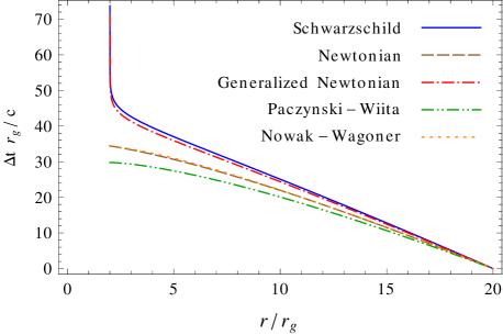
Figure 1: Infall time for a test particle falling radially from infinity as calculated in general relativity and using the potentials $\Phi_{\text{\tiny$\mathrm{N}$ }}$, $\Phi_{\text{\tiny$\mathrm{G}$ }}$, $\Phi_{\text{\tiny$\mathrm{PW}$ }}$, and $\Phi_{\text{\tiny$\mathrm{NW}$ }}$. In all the cases we have taken $\dot{r}_{\text{\tiny$\infty$ }}=-0.3\,\mathrm{c}$ and have chosen $r=20\,r_{\text{\tiny$\mathrm{g}$ }}$ as the synchronization radius. Note that both $\Delta t_{\text{\tiny$\mathrm{G}$ }}$ and $\Delta t_{\text{\tiny$\mathrm{S}$ }}$ diverge to infinity as the particle approaches the black hole horizon located at $r=2\,r_{\text{\tiny$\mathrm{g}$ }}$.

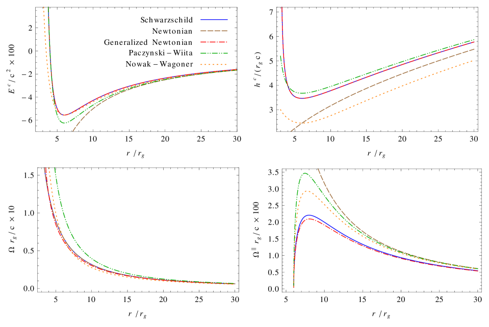
Figure 2: Comparison of different quantities associated with circular motion. From left to right and top to bottom the panels show the specific energy $E^{c}$, the specific angular momentum $h^{c}$, the orbital angular velocity $\Omega$, and the epicyclic frequency for small perturbations parallel to the orbital plane $\Omega^{\parallel}$. Note that the curves for $E^{c}_{\text{\tiny$\mathrm{G}$ }}$ and $E^{c}_{\text{\tiny$\mathrm{S}$ }}$ , $h^{c}_{\text{\tiny$\mathrm{G}$ }}$ and $h^{c}_{\text{\tiny$\mathrm{S}$ }}$ , and $\Omega_{\text{\tiny$\mathrm{N}$ }}$ and $\Omega_{\text{\tiny$\mathrm{S}$ }}$ lie on top of each other. Analytic expressions for the different quantities plotted in this figure are collected in Appendix B.

3.1 Radial infall

Consider a particle in radial free-fall, i.e. $\dot{\phi}=\dot{\theta}=0$. From Eq. (2.13) it follows that the amount of time that it takes for the particle to fall from a radius $r_{\text{\tiny$2$ }}$ to a smaller radius $r_{\text{\tiny$1$ }}$ is given by

$$\Delta t_{\text{\tiny$\mathrm{G}$ }}=\int_{r_{\text{\tiny$1$ }}}^{r_{\text{\tiny$2$ }}}\left[\left(1-\frac{2\,r_{\text{\tiny$\mathrm{g}$ }}}{r}\right)\sqrt{2\,E_{\text{\tiny$\mathrm{G}$ }}+\frac{2\,\mathrm{G}M}{r}}\right]^{-1}\mathrm{d}r.$$ (3.1)

It is clear that $\Delta t_{\text{\tiny$\mathrm{G}$ }}$ will coincide with the corresponding relativistic value $\Delta t_{\text{\tiny$\mathrm{S}$ }}$ (as calculated from Eq. 2.5) only when $E_{\text{\tiny$\mathrm{S}$ }}=E_{\text{\tiny$\mathrm{G}$ }}=0$, i.e. for a vanishing radial velocity at infinity. In the general case, we will have $\Delta t_{\text{\tiny$\mathrm{G}$ }}>\Delta t_{\text{\tiny$\mathrm{S}$ }}$ if $E_{\text{\tiny$\mathrm{G}$ }}<0$ and $\Delta t_{\text{\tiny$\mathrm{G}$ }}<\Delta t_{\text{\tiny$\mathrm{S}$ }}$ if $E_{\text{\tiny$\mathrm{G}$ }}>0$. Also note that both $\Delta t_{\text{\tiny$\mathrm{G}$ }}$ and $\Delta t_{\text{\tiny$\mathrm{S}$ }}$ diverge as $r_{\text{\tiny$1$ }}\rightarrow 2\,r_{\text{\tiny$\mathrm{g}$ }}$, which coincides with the description made by an observer situated at spatial infinity in Schwarzschild spacetime. In Fig. 1, we show the infall time as calculated from the relativistic solution and compare it with those coming from the use of $\Phi_{\text{\tiny$\mathrm{N}$ }}$, $\Phi_{\text{\tiny$\mathrm{G}$ }}$, $\Phi_{\text{\tiny$\mathrm{PW}$ }}$, and $\Phi_{\text{\tiny$\mathrm{NW}$ }}$.

3.2 Circular orbits

We consider now the special case of circular orbits as defined by the conditions

$$\dot{r}=0\quad\text{and}\quad\ddot{r}=0.$$ (3.2)

After substituting these two conditions into Eqs. (2.13) and (2.14) we get a system of two equations that can be solved for the corresponding values of $h_{\text{\tiny$\mathrm{G}$ }}$ and $E_{\text{\tiny$\mathrm{G}$ }}$ as

$$h^{c}_{\text{\tiny$\mathrm{G}$ }}=\frac{\sqrt{\mathrm{G}M}\,r}{\sqrt{r-3\,r_{\text{\tiny$\mathrm{g}$ }}}},$$ (3.3)

$$E^{c}_{\text{\tiny$\mathrm{G}$ }}=-\frac{\mathrm{G}M}{2\,r}\left(\frac{r-4\,r_{\text{\tiny$\mathrm{g}$ }}}{r-3\,r_{\text{\tiny$\mathrm{g}$ }}}\right),$$ (3.4)

which are identical to the relativistic expressions and lead to the exact locations for the corresponding photon orbit $r_{\text{\tiny$\mathrm{ph}$ }}=3\,r_{\text{\tiny$\mathrm{g}$ }}$ (at which both $h^{c}_{\text{\tiny$\mathrm{G}$ }}$ and $E^{c}_{\text{\tiny$\mathrm{G}$ }}$ diverge), the marginally bound orbit $r_{\text{\tiny$\mathrm{mb}$ }}=4\,r_{\text{\tiny$\mathrm{g}$ }}$ (for which $E^{c}_{\text{\tiny$\mathrm{G}$ }}=0$), and the marginally stable orbit $r_{\text{\tiny$\mathrm{ms}$ }}=6\,r_{\text{\tiny$\mathrm{g}$ }}$ (at which both $h^{c}_{\text{\tiny$\mathrm{G}$ }}$ and $E^{c}_{\text{\tiny$\mathrm{G}$ }}$ reach their minima). See the top panels of Figure 2 for a comparison of $E^{c}$ and $h^{c}$ as calculated using the different potentials.

On the other hand, by combining Eqs. (2.12) and (3.3) one finds the orbital angular velocity

$$\Omega_{\text{\tiny$\mathrm{G}$ }}=\sqrt{\frac{\mathrm{G}M}{r-3\,r_{\text{\tiny$\mathrm{g}$ }}}}\left(\frac{r-2\,r_{\text{\tiny$\mathrm{g}$ }}}{r^{2}}\right),$$ (3.5)

which should be compared against the exact expression in Schwarzschild spacetime

$$\Omega_{\text{\tiny$\mathrm{S}$ }}=\sqrt{\frac{\mathrm{G}M}{r^{3}}}.$$ (3.6)

For $r\geq 6\,r_{\text{\tiny$\mathrm{g}$ }}$, $\Omega_{\text{\tiny$\mathrm{G}$ }}$ reproduces the exact value with an accuracy better than $5.7\%$. In the bottom-left panel of Figure 2 we compare these two frequencies as well as the ones corresponding to the potentials $\Phi_{\text{\tiny$\mathrm{N}$ }}$, $\Phi_{\text{\tiny$\mathrm{PW}$ }}$, and $\Phi_{\text{\tiny$\mathrm{NW}$ }}$. The analytic expressions of all of the different quantities plotted in this figure are summarized in Appendix B.

3.3 Perturbed circular orbits

We now calculate the epicyclic frequencies associated with a small perturbation of a stable circular orbit in the equatorial plane. The unperturbed trajectory satisfies

$$x^{\text{\tiny$i$ }}(t) =(r,\pi/2,\Omega_{\text{\tiny$\mathrm{G}$ }}\,t),$$

$$\dot{x}^{\text{\tiny$i$ }}(t) =(0,0,\Omega_{\text{\tiny$\mathrm{G}$ }}),$$ (3.7)

while for the perturbed trajectory we have

$${x^{\prime}}^{\text{\tiny$i$ }}(t) =(r+\delta r,\pi/2+\delta\theta,\Omega_{\text{\tiny$\mathrm{G}$ }}\,t+\delta\phi),$$

$$\dot{x^{\prime}}^{\text{\tiny$i$ }}(t) =(\delta\dot{r},\delta\dot{\theta},\Omega_{\text{\tiny$\mathrm{G}$ }}+\delta\dot{\phi}).$$ (3.8)

Substituting these expressions into Eqs. (2.14)-(2.16) we obtain the following system of (linearized) differential equations for the perturbed quantities

$$\delta\ddot{r} =\left[\Omega^{2}_{\text{\tiny$\mathrm{G}$ }}+\frac{2\,\mathrm{G}M}{r^{5}}(r-2\,r_{\text{\tiny$\mathrm{g}$ }})(r-4\,r_{\text{\tiny$\mathrm{g}$ }})\right]\delta r$$

$$\hskip 12.0pt+2\,\Omega_{\text{\tiny$\mathrm{G}$ }}(r-3\,r_{\text{\tiny$\mathrm{g}$ }})\delta\dot{\phi},$$ (3.9)

$$\delta\ddot{\theta} =-\Omega^{2}_{\text{\tiny$\mathrm{G}$ }}\,\delta\theta$$ (3.10)

$$\delta\ddot{\phi} =-\frac{2\,\Omega_{\text{\tiny$\mathrm{G}$ }}}{r}\left(\frac{r-3\,r_{\text{\tiny$\mathrm{g}$ }}}{r-2\,r_{\text{\tiny$\mathrm{g}$ }}}\right)\delta\dot{r}.$$ (3.11)

From Eq. (3.10) we see that, to first order, the vertical perturbation decouples from the other two directions and has the same angular frequency as the orbital motion, i.e.

$$\Omega^{\perp}_{\text{\tiny$\mathrm{G}$ }}=\Omega_{\text{\tiny$\mathrm{G}$ }},$$ (3.12)

as is also the case for Schwarzschild spacetime. On the other hand, from Eqs. (3.9) and (3.11) we can see that the radial and azimuthal perturbations are coupled. Following Semerák & Žáček (2000), we assume that the solution to both equations is a harmonic oscillator with common angular frequency $\Omega^{\parallel}_{\text{\tiny$\mathrm{G}$ }}$, i.e. $\delta r=\delta r_{\text{\tiny$0$ }}\,{\rm e}^{i\,\Omega^{\parallel}_{\text{\tiny$\mathrm{G}$ }}\,t}$ and $\delta\phi=\delta\phi_{\text{\tiny$0$ }}\,{\rm e}^{i\,\Omega^{\parallel}_{\text{\tiny$\mathrm{G}$ }}\,t}$, where $\delta r_{\text{\tiny$0$ }}$ and $\delta\phi_{\text{\tiny$0$ }}$ are constant amplitudes. After substituting these solutions into Eqs. (3.9) and (3.11) we get as the only non-trivial solution

$$\Omega^{\parallel}_{\text{\tiny$\mathrm{G}$ }}=\sqrt{\frac{\mathrm{G}M}{r^{5}}\left(\frac{r-6\,r_{\text{\tiny$\mathrm{g}$ }}}{r-3\,r_{\text{\tiny$\mathrm{g}$ }}}\right)}(r-2\,r_{\text{\tiny$\mathrm{g}$ }}),$$ (3.13)

which should be compared against the exact relativistic value

$$\Omega^{\parallel}_{\text{\tiny$\mathrm{S}$ }}=\sqrt{\frac{\mathrm{G}M}{r^{3}}\left(1-\frac{6\,r_{\text{\tiny$\mathrm{g}$ }}}{r}\right)}.$$ (3.14)

Again, for $r\geq 6\,r_{\text{\tiny$\mathrm{g}$ }}$, $\Omega^{\parallel}_{\text{\tiny$\mathrm{G}$ }}$ reproduces the exact value with an accuracy better than $5.7\%$ (see the bottom-right panel of Figure 2).

Note that, even though none of the three frequencies $\Omega_{\text{\tiny$\mathrm{G}$ }}$, $\Omega^{\perp}_{\text{\tiny$\mathrm{G}$ }}$, and $\Omega^{\parallel}_{\text{\tiny$\mathrm{G}$ }}$ coincides with the corresponding relativistic expressions, they do keep the same ratios, i.e.

$$\frac{\Omega^{\perp}_{\text{\tiny$\mathrm{G}$ }}}{\Omega_{\text{\tiny$\mathrm{G}$ }}}=\frac{\Omega^{\perp}_{\text{\tiny$\mathrm{S}$ }}}{\Omega_{\text{\tiny$\mathrm{S}$ }}}=1\qquad\text{and}\qquad\frac{\Omega^{\parallel}_{\text{\tiny$\mathrm{G}$ }}}{\Omega_{\text{\tiny$\mathrm{G}$ }}}=\frac{\Omega^{\parallel}_{\text{\tiny$\mathrm{S}$ }}}{\Omega_{\text{\tiny$\mathrm{S}$ }}}=\sqrt{1-\frac{6\,r_{\text{\tiny$\mathrm{g}$ }}}{r}}.$$ (3.15)

The pseudo-Newtonian potential introduced by Kluźniak & Lee (2002) also reproduces exactly the ratio $\Omega^{\parallel}/\Omega$, although it does not reproduce satisfactorily other important features (e.g. one obtains $r_{\text{\tiny$\mathrm{ms}$ }}=3\,r_{\text{\tiny$\mathrm{g}$ }}$, $r_{\text{\tiny$\mathrm{mb}$ }}=1.3\,r_{\text{\tiny$\mathrm{g}$ }}$, and a p.e. of $\sim 42\%$ for the binding energy).

3.4 Non-Keplerian circular orbits

Consider a test particle going round a circular orbit with uniform angular velocity $\Omega=\mathrm{d}\phi/\mathrm{d}t$. This velocity does not necessarily coincide with the Keplerian value and, if it does not, an external radial force must be continuously applied in order to keep it on this circular trajectory. The actual nature of this force (e.g. pressure gradients, electromagnetic or propulsion from a rocket) is unimportant for the present discussion. We can calculate the necessary radial thrust from Eq. (2.14) as

$$\mathcal{F}_{\text{\tiny$\mathrm{G}$ }}=\frac{\mathrm{G}M}{r^{2}}\left(1-\frac{2\,r_{\text{\tiny$\mathrm{g}$ }}}{r}\right)^{2}-\Omega^{2}(r-3\,r_{\text{\tiny$\mathrm{g}$ }}).$$ (3.16)

On the other hand, the corresponding relativistic expression is given by

$$\mathcal{F}_{\text{\tiny$\mathrm{S}$ }}=a^{\text{\tiny$\hat{r}$ }}=\left(1-\frac{2\,r_{\text{\tiny$\mathrm{g}$ }}}{r}\right)^{\nicefrac{{-1}}{{2}}}a^{\text{\tiny$r$ }},$$ (3.17)

where $a^{\text{\tiny$\hat{r}$ }}$ is the physical value of the radial component of the four-acceleration $a^{\text{\tiny$\mu$ }}=u^{\text{\tiny$\nu$ }}u^{\text{\tiny$\mu$ }}_{\text{\tiny$;\nu$ }}$ (i.e. as projected along the radial direction of a local tetrad). Writing the four-velocity of the test particle as $u^{\text{\tiny$\mu$ }}=u^{\text{\tiny$t$ }}(1,0,0,\Omega)$, it is simple to check that the only non-vanishing component of the four-acceleration is

$$a^{\text{\tiny$r$ }}=\left(1-\frac{2\,r_{\text{\tiny$\mathrm{g}$ }}}{r}\right)\frac{\mathrm{G}M/r^{2}-r\,\Omega^{2}}{1-2\,r_{\text{\tiny$\mathrm{g}$ }}/r-r^{2}\Omega^{2}/\mathrm{c}^{2}},$$ (3.18)

from where we can rewrite Eq. (3.17) as

$$\mathcal{F}_{\text{\tiny$\mathrm{S}$ }}=\left[\frac{\mathrm{G}M}{r^{2}}-\frac{\Omega^{2}(r-3\,r_{\text{\tiny$\mathrm{g}$ }})}{1-2\,r_{\text{\tiny$\mathrm{g}$ }}/r-r^{2}\Omega^{2}/c^{2}}\right]\left(1-\frac{2\,r_{\text{\tiny$\mathrm{g}$ }}}{r}\right)^{\nicefrac{{-1}}{{2}}}.$$ (3.19)

In Figure 3 we compare $\mathcal{F}$ as obtained from the different potentials for $\Omega=0$, i.e. for a rocket that remains static at a fixed radius. From this figure we see that $\mathcal{F}_{\text{\tiny$\mathrm{G}$ }}$ gives the worst approximation to the relativistic value (p.e. $\leqslant 64\%$ for $r>6\,r_{\text{\tiny$\mathrm{g}$ }}$). In particular, note that $\mathcal{F}_{\text{\tiny$\mathrm{S}$ }}$ diverges to infinity as $r\rightarrow 2\,r_{\text{\tiny$\mathrm{g}$ }}$ while $\mathcal{F}_{\text{\tiny$\mathrm{G}$ }}$ vanishes at this radius. However, the behaviour of $\mathcal{F}_{\text{\tiny$\mathrm{G}$ }}$ is in qualitative agreement with the relativistic expression for $\ddot{r}\ (=\mathrm{G}M(r-2\,r_{\text{\tiny$\mathrm{g}$ }})/r^{3})$ which is a clear indication that the description made using $\Phi_{\text{\tiny$\mathrm{G}$ }}$ does not correspond to a local observer but rather to one located at spatial infinity.

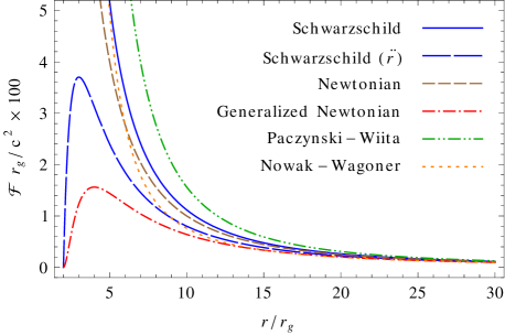
Figure 3: Radial thrust needed to keep a rocket hovering at a fixed radius. Note that $\mathcal{F}_{\text{\tiny$\mathrm{G}$ }}$ qualitatively follows the relativistic value of $\ddot{r}$ and vanishes at the event horizon ($r=2\,r_{\text{\tiny$\mathrm{g}$ }}$). This is not a physical result but rather a reflection of the fact that the Schwarzschild coordinates are ill-behaved at this radius.

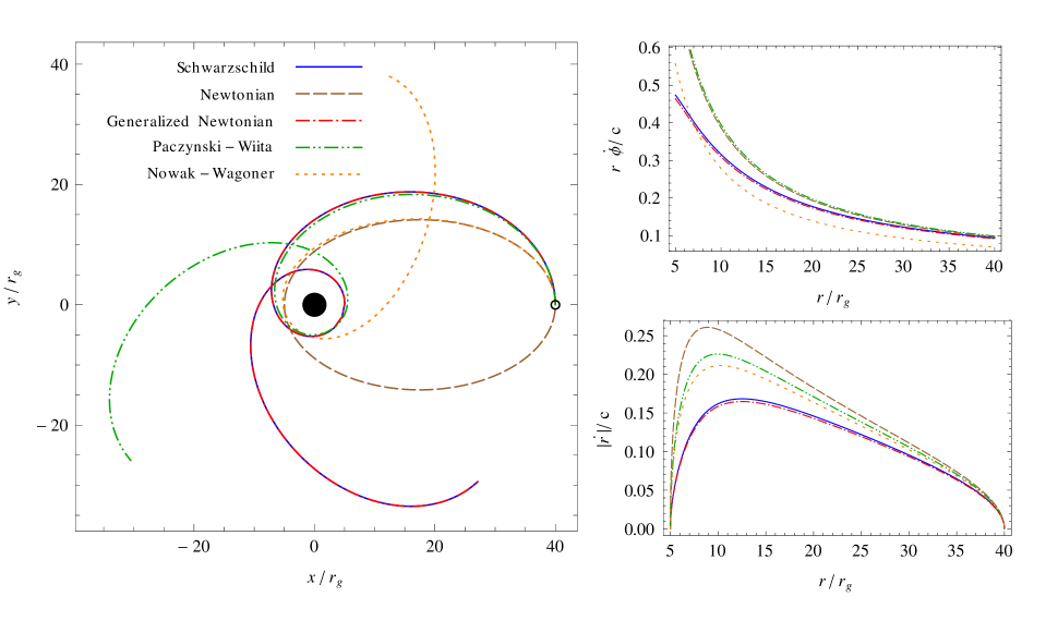
Figure 4: Comparison of an elliptic-like trajectory in Schwarzschild spacetime with those obtained using $\Phi_{\text{\tiny$\mathrm{N}$ }}$, $\Phi_{\text{\tiny$\mathrm{G}$ }}$, $\Phi_{\text{\tiny$\mathrm{PW}$ }}$, and $\Phi_{\text{\tiny$\mathrm{NW}$ }}$. In all the cases, the pericentre and apocentre of the orbit have been fixed as $r_{\text{\tiny$p$ }}=5\,r_{\text{\tiny$\mathrm{g}$ }}$ and $r_{\text{\tiny$a$ }}=40\,r_{\text{\tiny$\mathrm{g}$ }}$, respectively. The common initial point is indicated by an open circle. The left-hand panel shows the spatial projection of the different trajectories onto the $x$-$y$ plane (with $x=r\cos\varphi$ and $y=r\sin\varphi$). The panels on the right-hand side show the corresponding azimuthal (top) and radial (bottom) velocities as functions of the radius. Note that the spatial projection of the trajectory associated with the potential $\Phi_{\text{\tiny$\mathrm{G}$ }}$ reproduces exactly the relativistic one, while the velocities are very well approximated.

Note that Eq. (3.16) captures an important feature of the exact relativistic expression in Eq. (3.19), namely that the radial thrust becomes independent of the angular velocity at the location of the circular photon orbit $r=3\,r_{\text{\tiny$\mathrm{g}$ }}$ (Abramowicz & Lasota, 1986), and that the centrifugal force reverses sign at this radius (Abramowicz, 1990). As Abramowicz & Miller (1990) pointed out, a consequence of this effect is the general relativistic result that the ellipticity of a slowly rotating Maclaurin spheroid changes monotonicity at $r\approx 5\,r_{\text{\tiny$\mathrm{g}$ }}$ as the spheroid contracts with constant mass and angular momentum (whereas in the Newtonian case the ellipticity monotonically increases as the mean radius of the shrinking body decreases) (Chandrasekhar & Miller, 1974; Miller, 1977). Following the same approach as in Abramowicz & Miller (1990), it is simple to check that the present Newtonian description leads to the same expression for the ellipticity as their Eq. (12’) that quantitatively reproduces this effect (p.e. $\leqslant 35\%$ for $r>4\,r_{\text{\tiny$\mathrm{g}$ }}$).

3.5 General orbits and pericentre advance

The geometric description of the trajectory followed by a test particle is obtained by combining Eqs. (2.12) and (2.13) as

$$\frac{\mathrm{d}r}{\mathrm{d}\varphi}=\frac{\sqrt{P(r)}}{h_{\text{\tiny$\mathrm{G}$ }}},$$ (3.20)

where

$$P(r)=2\,E_{\text{\tiny$\mathrm{G}$ }}\,r^{4}+2\,\mathrm{G}Mr^{3}-h^{2}_{\text{\tiny$\mathrm{G}$ }}\,r\left(r-2\,r_{\text{\tiny$\mathrm{g}$ }}\right).$$ (3.21)

Eq. (3.20) is formally identical to the general relativistic expressions once the correspondences

$$E_{\text{\tiny$\mathrm{G}$ }}\leftrightarrow E_{\text{\tiny$\mathrm{S}$ }}\qquad\text{and}\qquad h_{\text{\tiny$\mathrm{G}$ }}\leftrightarrow h_{\text{\tiny$\mathrm{S}$ }}$$ (3.22)

have been taken. This means that the spatial projection of the trajectories obtained with $\Phi_{\text{\tiny$\mathrm{G}$ }}$ is identical to that coming from the full Schwarzschild solution. In other words, the orbital parameters (e.g. apocentre, pericentre, eccentricity) and characteristics (e.g. pericentre advance, whether it is bound, unbound or eventually trapped) have the same functional dependence on the corresponding constants of motion. In Figure 4, we show an example of a generic elliptic-like trajectory as resulting from the full general relativistic solution and compare it with those coming from the use of $\Phi_{\text{\tiny$\mathrm{N}$ }}$, $\Phi_{\text{\tiny$\mathrm{G}$ }}$, $\Phi_{\text{\tiny$\mathrm{PW}$ }}$, and $\Phi_{\text{\tiny$\mathrm{NW}$ }}$.

Just as in the general relativistic case, the solution to Eq. (3.20) can be written in terms of elliptic integrals (see e.g. Chandrasekhar, 1983; Tejeda et al., 2012). In the particular case of a bound orbit (elliptic-like trajectory) such that $r\in[r_{\text{\tiny$p$ }},r_{\text{\tiny$a$ }}]$ (where $r_{\text{\tiny$p$ }}$ and $r_{\text{\tiny$a$ }}$ are the pericentre and apocentre of the orbit, respectively), we define its (half) orbital period as

$$\Pi_{\text{\tiny$\mathrm{G}$ }}=\int_{r_{\text{\tiny$p$ }}}^{r_{\text{\tiny$a$ }}}\frac{h_{\text{\tiny$\mathrm{G}$ }}\,\mathrm{d}r}{\sqrt{P(r)}}=\frac{2\,h_{\text{\tiny$\mathrm{G}$ }}\,K(k)}{\sqrt{-2\,E_{\text{\tiny$\mathrm{G}$ }}\,r_{\text{\tiny$p$ }}(r_{\text{\tiny$a$ }}-r_{\text{\tiny$b$ }})}},$$ (3.23)

where $K(k)$ is the complete elliptic integral of the first kind whose modulus $k$ is given by

$$k=\sqrt{\frac{r_{\text{\tiny$b$ }}(r_{\text{\tiny$a$ }}-r_{\text{\tiny$p$ }})}{r_{\text{\tiny$p$ }}(r_{\text{\tiny$a$ }}-r_{\text{\tiny$b$ }})}},$$ (3.24)

and $r_{\text{\tiny$b$ }}=\mathrm{G}M/E_{\text{\tiny$\mathrm{G}$ }}-r_{\text{\tiny$a$ }}-r_{\text{\tiny$p$ }}$ is the smallest positive root of $P(r)$. The pericentre advance or precession is given by

$$\text{pericentre advance}=\Pi_{\text{\tiny$\mathrm{G}$ }}-\pi.$$ (3.25)

It is simple to check that, in the non-relativistic limit, $r_{\text{\tiny$b$ }}\rightarrow 0$ and, thus, $k\rightarrow 0$. Given that $K(0)=\pi/2$, it follows then from Eq. (3.23) that

$$\Pi_{\text{\tiny$\mathrm{G}$ }}\xrightarrow[\rm nrl]{}\pi.$$ (3.26)

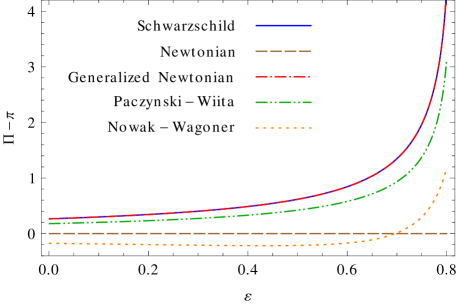
Figure 5: Pericentre advance as a function of the eccentricity $\varepsilon$ for a fixed apocentre $r_{\text{\tiny$a$ }}=40\,r_{\text{\tiny$\mathrm{g}$ }}$. Note that $\Phi_{\text{\tiny$\mathrm{G}$ }}$ reproduces exactly the relativistic value, while the result obtained with $\Phi_{\text{\tiny$\mathrm{PW}$ }}$ is consistently below the exact value by $\sim 30\%$. On the other hand, for most values of $\varepsilon$, $\Phi_{\text{\tiny$\mathrm{NW}$ }}$ produces a negative shift.

In Figure 5, we have plotted the pericentre advance as a function of the eccentricity $\varepsilon=(r_{\text{\tiny$a$ }}-r_{\text{\tiny$p$ }})/(r_{\text{\tiny$a$ }}+r_{\text{\tiny$p$ }})$ as predicted by general relativity, $\Phi_{\text{\tiny$\mathrm{N}$ }}$, $\Phi_{\text{\tiny$\mathrm{G}$ }}$, $\Phi_{\text{\tiny$\mathrm{PW}$ }}$, and $\Phi_{\text{\tiny$\mathrm{NW}$ }}$. As already mentioned, the pericentre advance resulting from $\Phi_{\text{\tiny$\mathrm{G}$ }}$ corresponds to the exact relativistic value. On the other hand, the pericentre advance obtained from $\Phi_{\text{\tiny$\mathrm{PW}$ }}$ is off by $\sim 30\%$, while, for most values of the eccentricity, $\Phi_{\text{\tiny$\mathrm{NW}$ }}$ yields a negative shift (i.e. a pericentre lag rather than an advance).

The pseudo-Newtonian potential introduced by Wegg (2012) was specifically designed to give an accurate description of the pericentre shift for parabolic-like trajectories (p.e. $\leqslant 1\%$). Nevertheless, this potential is not well suited for studying more general cases (for instance, it does not give the correct location of either $r_{\text{\tiny$\mathrm{ms}$ }}$ or $r_{\text{\tiny$\mathrm{mb}$ }}$).

3.6 Accretion disc

In this section we consider the simple model of the stationary, geometrically thin and optically thick accretion disc first investigated by Shakura & Sunyaev (1973) in a Newtonian context and its extension to a Schwarzschild spacetime by Novikov & Thorne (1973). Under the assumptions used there, it turns out that the energy flux per unit area from the disc surface depends on the mass flux but not on the details of the viscosity prescription and is given by (see e.g. Frank et al., 2002)

$$D=\frac{\dot{M}}{4\,\pi\,r}\left|\frac{\mathrm{d}\Omega}{\mathrm{d}r}\right|\left[h(r)-h(r_{\text{\tiny$\mathrm{in}$ }})\right],$$ (3.27)

where $\dot{M}$ is the constant accretion rate and $r_{\text{\tiny$\mathrm{in}$ }}$ is the inner boundary of the disc at which the viscous stresses are assumed to vanish. In the standard thin disc model, one takes $r_{\text{\tiny$\mathrm{in}$ }}=r_{\text{\tiny$\mathrm{ms}$ }}$. The total luminosity from the two faces of the disc is obtained after integrating Eq. (3.27) over the whole disc, i.e.

$$L=2\int_{r_{\text{\tiny$\mathrm{in}$ }}}^{\infty}D(r)\,2\,\pi\,r\,\mathrm{d}r=e\dot{M}\mathrm{c}^{2},$$ (3.28)

where $e$ is called the efficiency of the accretion process. In the following list, we give the values of $e$ for the different potentials

$$\begin{split}&e_{\text{\tiny$\mathrm{N}$ }}=-E_{\text{\tiny$\mathrm{N}$ }}(r_{\text{\tiny$\mathrm{in}$ }})/\mathrm{c}^{2}=\frac{1}{12}\simeq 0.083,\\ &e_{\text{\tiny$\mathrm{PW}$ }}=-E_{\text{\tiny$\mathrm{PW}$ }}(r_{\text{\tiny$\mathrm{in}$ }})/\mathrm{c}^{2}=\frac{1}{16}\simeq 0.062,\\ &e_{\text{\tiny$\mathrm{NW}$ }}=-E_{\text{\tiny$\mathrm{NW}$ }}(r_{\text{\tiny$\mathrm{in}$ }})/\mathrm{c}^{2}=\frac{1}{18}\simeq 0.056,\\ &e_{\text{\tiny$\mathrm{G}$ }}=-E_{\text{\tiny$\mathrm{G}$ }}(r_{\text{\tiny$\mathrm{in}$ }})/\mathrm{c}^{2}=\frac{1}{18}\simeq 0.056,\\ &e_{\text{\tiny$\mathrm{S}$ }}=1-\mathcal{E}(r_{\text{\tiny$\mathrm{in}$ }})/\mathrm{c}^{2}=1-\frac{2\sqrt{2}}{3}\simeq 0.057,\end{split}$$ (3.29)

from where we see that $\Phi_{\text{\tiny$\mathrm{NW}$ }}$ and $\Phi_{\text{\tiny$\mathrm{G}$ }}$ give an equally good approximation to the relativistic value. Nonetheless, for the actual radial dependence of $D$, the latter provides a better approximation (p.e. $\leqslant 7.2\%$) than the former (p.e. $\leqslant 11\%$). In Figure 6, we compare $D$ as obtained from general relativity with the results from the various potentials.

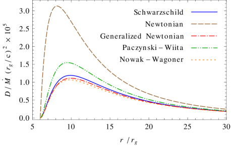
Figure 6: Energy flux per unit area $D$ as a function of radius emitted from the surface of a geometrically thin, optically thick accretion disc.

3.7 Accretion inflow

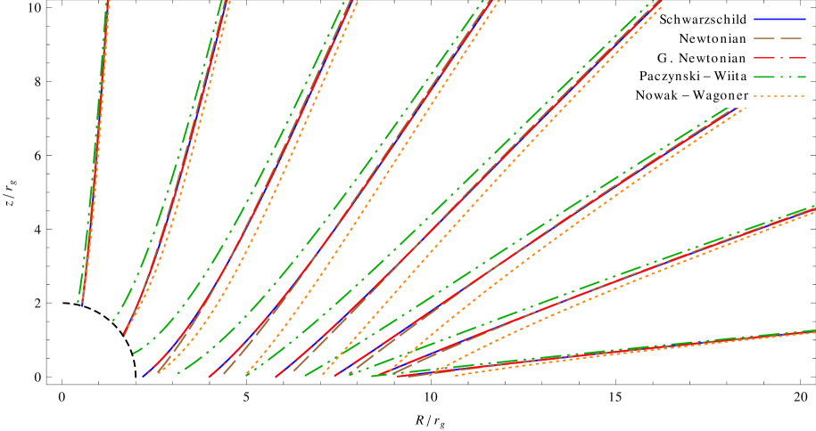
Figure 7: Streamlines of the steady-state accretion flow of a rotating gas cloud of non-interacting particles onto a Schwarzschild black hole. The boundary conditions are as given in Eq. (3.30). The figure shows a zoom-in of the first quadrant of the $R$-$z$ plane (with $R=r\,\sin\theta$ and $z=r\,\cos\theta$). The black hole horizon is indicated with the dashed-line quarter circle.

Here we consider the analytic accretion model of Tejeda et al. (2012) and Tejeda et al. (2013). In this model a rotating gas cloud of non-interacting particles accretes steadily onto a Schwarzschild black hole. In Figure 7, we compare the streamlines of the relativistic solution with the ones obtained from the potentials $\Phi_{\text{\tiny$\mathrm{N}$ }}$, $\Phi_{\text{\tiny$\mathrm{G}$ }}$, $\Phi_{\text{\tiny$\mathrm{PW}$ }}$, and $\Phi_{\text{\tiny$\mathrm{NW}$ }}$ for the following set of boundary conditions:

$$\begin{split}M&=4\,\mathrm{M}_{\odot},\\ \dot{M}&=0.01\,\mathrm{M}_{\odot}/s,\\ r_{\text{\tiny$0$ }}&=100\,r_{\text{\tiny$\mathrm{g}$ }},\\ \dot{r}_{\text{\tiny$0$ }}&=-0.141\,\mathrm{c},\\ r_{\text{\tiny$0$ }}\,\dot{\phi}_{\text{\tiny$0$ }}&=0.038\,\mathrm{c},\\ \dot{\theta}_{\text{\tiny$0$ }}&=0.\end{split}$$ (3.30)

These boundary conditions are motivated by collapsing stellar cores leading to long gamma-ray bursts and were used in Tejeda et al. (2012) to make a comparison with one of the simulations of collapsar progenitors in Lee & Ramírez-Ruiz (2006).

Note that the streamlines obtained from $\Phi_{\text{\tiny$\mathrm{G}$ }}$ are basically indistinguishable from the exact relativistic ones. This is so because the energies of the incoming fluid elements are close to parabolic, i.e. $\mathcal{E}\simeq\mathrm{c}^{2}$ (for which case Eqs. (2.12) and (2.13) coincide with the exact relativistic equations). With a different choice of boundary conditions, the agreement with the relativistic results may not be as good as in Figure 7, although $\Phi_{\text{\tiny$\mathrm{G}$ }}$ is still in better agreement with the relativistic solution than $\Phi_{\text{\tiny$\mathrm{PW}$ }}$, $\Phi_{\text{\tiny$\mathrm{NW}$ }}$, or $\Phi_{\text{\tiny$\mathrm{N}$ }}$.

3.8 Tidal disruption

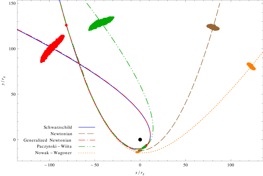
Figure 8: Tidal disruption of a solar-type star ($M_{\ast}=1\,\mathrm{M}_{\odot}$, $R_{\ast}=1\,\mathrm{R}_{\odot}$) by a supermassive black hole ($M_{\text{\tiny$\mathrm{BH}$ }}=10^{6}\,\mathrm{M}_{\odot}$). The figure shows the outcome of four runs of the same SPH code for each of the potentials $\Phi_{\text{\tiny$\mathrm{N}$ }}$, $\Phi_{\text{\tiny$\mathrm{G}$ }}$, $\Phi_{\text{\tiny$\mathrm{PW}$ }}$, and $\Phi_{\text{\tiny$\mathrm{NW}$ }}$. A common initial configuration is used in which the star is set at $r=200\,r_{\text{\tiny$\mathrm{g}$ }}$ along a parabolic trajectory with an encounter strength of $\beta=5$. Only $10^{4}$ SPH particles were used for each simulation. The figure also shows the trajectory followed by the centre of mass of the star in each case (as projected onto the orbital plane), together with the projection of the SPH particles at three different points of the trajectory. For reference, we also show with a solid blue line the exact geodesic trajectory of a test particle in Schwarzschild spacetime.

In this section we apply the generalized potential to the tidal disruption of a main-sequence star by a supermassive black hole. For doing this, we have implemented the acceleration given in Eq. (A.5) within the Newtonian SPH code that we had used previously to simulate the tidal disruption of white dwarf stars by moderately massive black holes (Rosswog et al., 2009) and which has been described in detail in Rosswog et al. (2008). For recent reviews of the SPH method see, e.g. Monaghan (2005) and Rosswog (2009).

It is worth mentioning that for use in an Eulerian hydrodynamics code, it may be beneficial to perform the simulation in the rest frame of the star to overcome geometric restrictions and to minimize numerical artefacts due to advection (e.g. Cheng & Evans, 2013; Guillochon & Ramirez-Ruiz, 2013). Such an approach may require a multipole expansion of the tidal field around the stellar centre, but this is beyond the scope of the current paper and left to future efforts.

Here we choose parameters that are identical to the ones of a general relativistic simulation run presented in Laguna et al. (1993): the masses are $M_{\text{\tiny$\mathrm{BH}$ }}=10^{6}\,\mathrm{M}_{\odot}$ for the black hole and $M_{\ast}=1\,\mathrm{M}_{\odot}$ for the star, the latter has a radius of $R_{\ast}=1\,\mathrm{R}_{\odot}$ and is modelled using a polytropic equation of state with exponent $\Gamma=5/3$. The star approaches the central black hole following a parabolic trajectory with an encounter strength $\beta=r_{\text{\tiny$\mathrm{t}$ }}/r_{\text{\tiny$p$ }}=5$, where $r_{\text{\tiny$\mathrm{t}$ }}=(M_{\text{\tiny$\mathrm{BH}$ }}/M_{\ast})^{1/3}R_{\ast}\simeq 47\,r_{\text{\tiny$\mathrm{g}$ }}$ is the tidal radius and $r_{\text{\tiny$p$ }}\simeq 9.4\,r_{\text{\tiny$\mathrm{g}$ }}$ is the pericentre distance. As in the previous test cases, we compare the results obtained with the generalized potential with those using $\Phi_{\text{\tiny$\mathrm{N}$ }}$, $\Phi_{\text{\tiny$\mathrm{PW}$ }}$, and $\Phi_{\text{\tiny$\mathrm{NW}$ }}$.

The results for the different approaches are displayed in Figure 8. For ease of comparison with Laguna et al. (1993), we simply show the trajectory followed by the centre of mass in each case together with the particle positions projected onto the orbital plane at three different points of the trajectories. Obviously, for such a deep encounter, relativistic effects lead to substantial deviations from the Newtonian parabola. In this case, $\Phi_{\text{\tiny$\mathrm{PW}$ }}$ produces a qualitatively correct result, although with only about $70\%$ of the relativistic pericentre advance. As expected based on Fig. 5, $\Phi_{\text{\tiny$\mathrm{NW}$ }}$ gives a pericentre shift with the opposite sign to that given by general relativity, and therefore leads to a wider orbit than the purely Newtonian potential. Although the star passes the black hole with about $0.4\,\mathrm{c}$, the hydrodynamic result obtained from $\Phi_{\text{\tiny$\mathrm{G}$ }}$ is in very close agreement with the geodesic in Schwarzschild spacetime and the matter distribution closely resembles the one shown in Laguna et al. (1993) (see their figure 1, second column).

4 Summary

We have derived a generalized Newtonian potential from the geodesic motion of a test particle in Schwarzschild spacetime in the low-energy limit $\mathcal{E}\simeq\mathrm{c}^{2}$. In addition to the standard Newtonian term, the generalized potential $\Phi_{\text{\tiny$\mathrm{G}$ }}$ includes a term that depends on the square of the velocity of the test particle and this can be interpreted as an additional gravitational attraction from the central mass acting on the kinetic energy of the test particle.

The new potential reproduces exactly several relativistic features of the motion of test particles in Schwarzschild spacetime such as: the location of the photon, marginally bound and marginally stable circular orbits; the radial dependence of the energy and angular momentum of circular orbits; the ratio between the orbital and epicyclic frequencies; the time evolution of parabolic-like trajectories; the spatial projection of general trajectories as function of the constants of motion and their pericentre advance. Moreover, the equations of motion derived from this potential reproduce the reversal of the centrifugal force at the location of the circular photon orbit (see e.g. Abramowicz, 1990). We are not aware of this relativistic feature ever having been reproduced before by any pseudo-Newtonian potential. Additionally, the equations obtained also provide a good approximation for the time evolution of particles in free-fall, for the orbital angular velocity of circular orbits, and for the epicyclic frequencies associated with small perturbations away from circular motion (all of these corresponding to the description made by observers situated far away from the central black hole). We have also applied $\Phi_{\text{\tiny$\mathrm{G}$ }}$ to the study of simple accretion scenarios, first for the thin disc model of Novikov & Thorne (1973) and then for the accretion infall model of Tejeda et al. (2012), finding good agreement with the exact relativistic solutions in both cases.

As a further astrophysical application and a demonstration of the minimal effort required to implement the suggested generalized potential within an existing Newtonian hydrodynamics code, we have applied it to the tidal disruption of a main-sequence star by a supermassive black hole. For this, we implemented the equations of motion derived from $\Phi_{\text{\tiny$\mathrm{G}$ }}$ within the 3D SPH code described in Rosswog et al. (2008). The results obtained are in very good agreement with the relativistic simulation presented in Laguna et al. (1993).

Potential	$\Phi_{\text{\tiny$\mathrm{N}$ }}$	$\Phi_{\text{\tiny$\mathrm{PW}$ }}$	$\Phi_{\text{\tiny$\mathrm{NW}$ }}$	$\Phi_{\text{\tiny$\mathrm{G}$ }}$
$\Delta t(\dot{r}_{\text{\tiny$\infty$ }}=0)$	$\leqslant 16.7\%$	$\leqslant 23.8\%$	$\leqslant 9.3\%$	exact
$\Delta t(\dot{r}_{\text{\tiny$\infty$ }}=-0.3\,c)$	$\leqslant 15.9\%$	$\leqslant 24.3\%$	$\leqslant 15\%$	$\leqslant 2.9\%$
$r_{\text{\tiny$\mathrm{ph}$ }}$	$-$	$33.3\%$	$-$	exact
$r_{\text{\tiny$\mathrm{mb}$ }}$	$-$	exact	$13.4\%$	exact
$r_{\text{\tiny$\mathrm{ms}$ }}$	$-$	exact	exact	exact
$E^{c}$	$\leqslant 50\%$	$\leqslant 12.5\%$	$\leqslant 3.3\%$	exact
$h^{c}$	$\leqslant 29.3\%$	$\leqslant 6.1\%$	$\leqslant 29.3\%$	exact
$\Omega$	exact	$\leqslant 50\%$	$\leqslant 13.4\%$	$\leqslant 5.7\%$
$\Omega^{\parallel}$	$\infty$	$\leqslant 83.7\%$	$\leqslant 41.4\%$	$\leqslant 5.7\%$
$\mathcal{F}$	$\leqslant 18.4\%$	$\leqslant 83.7\%$	$\leqslant 32.1\%$	$\leqslant 63.7\%$
$\Pi-\pi$	$-$	$\sim 30\%$	$>80\%$	exact
$e$	$45.7\%$	$9.3\%$	$2.9\%$	$2.9\%$
$D$	$\infty$	$\leqslant 58.9\%$	$\leqslant 11.1\%$	$\leqslant 7.3\%$

Table 1: Maximum percentage error obtained for the approximation of several quantities associated with the motion of test particles in Schwarzschild spacetime using the four potentials $\Phi_{\text{\tiny$\mathrm{N}$ }}$, $\Phi_{\text{\tiny$\mathrm{PW}$ }}$, $\Phi_{\text{\tiny$\mathrm{NW}$ }}$ and $\Phi_{\text{\tiny$\mathrm{G}$ }}$. In all cases, we have considered only $r>6\,r_{\text{\tiny$\mathrm{g}$ }}$.

In Table 1, we summarize the accuracy with which various relativistic properties are reproduced by $\Phi_{\text{\tiny$\mathrm{N}$ }}$, $\Phi_{\text{\tiny$\mathrm{PW}$ }}$, $\Phi_{\text{\tiny$\mathrm{NW}$ }}$, and $\Phi_{\text{\tiny$\mathrm{G}$ }}$. With the exception of the radial thrust $\mathcal{F}$ needed to keep a rocket hovering at a static position, we found that $\Phi_{\text{\tiny$\mathrm{G}$ }}$ provides a more accurate description of the motion of test particles in Schwarzschild spacetime than any of the other potentials. For this reason, and given that a proper modelling of a realistic accretion scenario requires that (at least) all of these relativistic features are accurately reproduced, we consider the new potential as being a promising simple but powerful tool for studying many processes occurring in the vicinity of a Schwarzschild black hole.

5 Acknowledgements

It is a pleasure to thank John C. Miller for insightful discussion and critical comments on the manuscript. We also thank Marek Abramowicz, Oleg Korobkin, Iván Zalamea and the anonymous referee for useful comments and suggestions. The simulations of this paper were in part performed on the facilities of the Höchstleistungsrechenzentrum Nord (HLRN). This work has been supported by the Swedish Research Council (VR) under grant 621-2012-4870.

Appendix A Acceleration in Cartesian coordinates

The Cartesian coordinates $(x,y,z)$ are connected to the spherical ones $(r,\theta,\phi)$ in the usual way, i.e.

$$x=r\,\sin\theta\cos\phi, r =\sqrt{x^{2}+y^{2}+z^{2}},$$

$$y=r\,\sin\theta\sin\phi, \theta =\tan^{-1}\left(\sqrt{x^{2}+y^{2}}/z\right),$$ (A.1)

$$z=r\,\cos\theta, \phi =\tan^{-1}\left(y/x\right),$$

from which we get

$$r\,\dot{r}=\ x\,\dot{x}+y\,\dot{y}+z\,\dot{z}=\sum_{\text{\tiny$i$ }}\,x^{\text{\tiny$i$ }}\,\dot{x}^{\text{\tiny$i$ }},$$ (A.2)

$$r^{4}(\dot{\theta}^{2}+\sin^{2}\theta\,\dot{\phi}^{2})=\ (x\,\dot{y}-y\,\dot{x})^{2}+(x\,\dot{z}-z\,\dot{x})^{2}+(z\,\dot{y}-y\,\dot{z})^{2}=\sum_{i}\left(\sum_{\text{\tiny$jk$ }}\epsilon_{\text{\tiny$ijk$ }}\,x^{\text{\tiny$j$ }}\,\dot{x}^{\text{\tiny$k$ }}\right)^{2},$$ (A.3)

where $x^{\text{\tiny$i$ }}=x,y,z$ and $\epsilon_{\text{\tiny$ijk$ }}$ is the Levi-Civita symbol. Substituting Eqs. (A.2) and (A.3) into the Lagrangian in Eq. (2.11) gives

$$L=\frac{1}{2}\left[\left(\frac{\sum_{\text{\tiny$i$ }}x^{\text{\tiny$i$ }}\,\dot{x}^{\text{\tiny$i$ }}}{r-2\,r_{\text{\tiny$\mathrm{g}$ }}}\right)^{2}+\frac{\sum_{\text{\tiny$i$ }}\left(\sum_{\text{\tiny$jk$ }}\epsilon_{\text{\tiny$ijk$ }}\,x^{\text{\tiny$j$ }}\,\dot{x}^{\text{\tiny$k$ }}\right)^{2}}{r(r-2\,r_{\text{\tiny$\mathrm{g}$ }})}\right]+\frac{\mathrm{G}M}{r},$$ (A.4)

from which we get the following expression for the acceleration components

$$\ddot{x}^{\text{\tiny$i$ }}=-\frac{\mathrm{G}Mx^{\text{\tiny$i$ }}}{r^{3}}\left(1-\frac{2\,r_{\text{\tiny$\mathrm{g}$ }}}{r}\right)^{2}+\frac{2\,r_{\text{\tiny$\mathrm{g}$ }}\,\dot{x}^{\text{\tiny$i$ }}}{r^{2}(r-2\,r_{\text{\tiny$\mathrm{g}$ }})}\,\sum_{j}\,x^{\text{\tiny$j$ }}\,\dot{x}^{\text{\tiny$j$ }}-\frac{3\,r_{\text{\tiny$\mathrm{g}$ }}\,x^{\text{\tiny$i$ }}}{r^{5}}\,\sum_{j}\bigg{(}\sum_{kl}\epsilon_{\text{\tiny$jkl$ }}\,x^{\text{\tiny$k$ }}\,\dot{x}^{\text{\tiny$l$ }}\bigg{)}^{2}.$$ (A.5)

Appendix B Miscellaneous expressions

In the following table we collect the different formulae associated with circular motion and plotted in Figures 2 and 3. The corresponding Newtonian expressions are also included to facilitate further comparison.

	Newton	Schwarzschild	Generalized Newtonian	Paczyński-Wiita	Nowak-Wagoner
$\mathcal{F}$	$-\frac{\mathrm{G}M}{r^{2}}$	$-\frac{\mathrm{G}M}{\sqrt{r^{3}(r-2\,r_{\text{\tiny$\mathrm{g}$ }})}}$	$-\frac{\mathrm{G}M(r-2\,r_{\text{\tiny$\mathrm{g}$ }})^{2}}{r^{4}}$	$-\frac{\mathrm{G}M}{(r-2\,r_{\text{\tiny$\mathrm{g}$ }})^{2}}$	$-\frac{\mathrm{G}M(r^{2}-6\,r_{\text{\tiny$\mathrm{g}$ }}\,r+36\,r^{2}_{\text{\tiny$g$ }})}{r^{4}}$
$(h^{c})^{2}$	${\scriptstyle\mathrm{G}Mr}$	$\frac{\mathrm{G}Mr^{2}}{r-3\,r_{\text{\tiny$\mathrm{g}$ }}}$	$\frac{\mathrm{G}Mr^{2}}{r-3\,r_{\text{\tiny$\mathrm{g}$ }}}$	$\frac{\mathrm{G}Mr^{3}}{(r-2\,r_{\text{\tiny$\mathrm{g}$ }})^{2}}$	$\frac{\mathrm{G}M(r^{2}-6\,r_{\text{\tiny$\mathrm{g}$ }}\,r+36\,r^{2}_{\text{\tiny$g$ }})}{r}$
$E^{c}$	$-\frac{\mathrm{G}M}{2\,r}$	$-\frac{\mathrm{G}M(r-4\,r_{\text{\tiny$\mathrm{g}$ }})}{2\,r(r-3\,r_{\text{\tiny$\mathrm{g}$ }})}$	$-\frac{\mathrm{G}M(r-4\,r_{\text{\tiny$\mathrm{g}$ }})}{2\,r(r-3\,r_{\text{\tiny$\mathrm{g}$ }})}$	$-\frac{\mathrm{G}M(r-4\,r_{\text{\tiny$\mathrm{g}$ }})}{2(r-2\,r_{\text{\tiny$\mathrm{g}$ }})^{2}}$	$-\frac{\mathrm{G}M(r^{2}-12\,r^{2}_{\text{\tiny$g$ }})}{2\,r^{3}}$
$\Omega^{2}$	$\frac{\mathrm{G}M}{r^{3}}$	$\frac{\mathrm{G}M}{r^{3}}$	$\frac{\mathrm{G}M(r-2\,r_{\text{\tiny$\mathrm{g}$ }})^{2}}{r^{4}(r-3\,r_{\text{\tiny$\mathrm{g}$ }})}$	$\frac{\mathrm{G}M}{r(r-2\,r_{\text{\tiny$\mathrm{g}$ }})^{2}}$	$\frac{\mathrm{G}M(r^{2}-6\,r_{\text{\tiny$\mathrm{g}$ }}\,r+36\,r^{2}_{\text{\tiny$g$ }})}{r^{5}}$
$(\Omega^{\text{\tiny$\parallel$ }})^{2}$	$\frac{\mathrm{G}M}{r^{3}}$	$\frac{\mathrm{G}M(r-6\,r_{\text{\tiny$g$ }})}{r^{4}}$	$\frac{\mathrm{G}M(r-6\,r_{\text{\tiny$g$ }})(r-2\,r_{\text{\tiny$\mathrm{g}$ }})^{2}}{r^{5}(r-3\,r_{\text{\tiny$g$ }})}$	$\frac{\mathrm{G}M(r-6\,r_{\text{\tiny$g$ }})}{r(r-2\,r_{\text{\tiny$\mathrm{g}$ }})^{3}}$	$\frac{\mathrm{G}M(r^{2}-36\,r^{2}_{\text{\tiny$g$ }})}{r^{5}}$

References

- Abramowicz (1990) Abramowicz M. A., 1990, Monthly Notices of the Royal Astronomical Society, 245, 733
- Abramowicz (2009) Abramowicz M. A., 2009, Astronomy and Astrophysics, 500, 213
- Abramowicz et al. (1988) Abramowicz M. A., Czerny B., Lasota J. P., Szuszkiewicz E., 1988, Astrophysical Journal, 332, 646
- Abramowicz et al. (1997) Abramowicz M. A., Lanza A., Miller J. C., Sonego S., 1997, General Relativity and Gravitation, 29, 1583
- Abramowicz & Lasota (1986) Abramowicz M. A., Lasota J. P., 1986, American Journal of Physics, 54, 936
- Abramowicz & Miller (1990) Abramowicz M. A., Miller J. C., 1990, Monthly Notices of the Royal Astronomical Society, 245, 729
- Artemova et al. (1996) Artemova I. V., Björnsson G., Novikov I. D., 1996, Astrophysical Journal, 461, 565
- Chakrabarti & Titarchuk (1995) Chakrabarti S., Titarchuk L. G., 1995, Astrophysical Journal, 455, 623
- Chandrasekhar (1983) Chandrasekhar S., 1983, The Mathematical Theory of Black Holes. Oxford University Press
- Chandrasekhar & Miller (1974) Chandrasekhar S., Miller J. C., 1974, Monthly Notices of the Royal Astronomical Society, 167, 63
- Cheng & Evans (2013) Cheng R. M., Evans C. R., 2013, Physical Review D, 87, 104010
- Frank et al. (2002) Frank J., King A., Raine D., 2002, Accretion Power in Astrophysics, 3rd edn. Cambridge University Press
- Frolov & Novikov (1998) Frolov V. P., Novikov I. D., 1998, Black Hole Physics: Basic Concepts and New Developments. Kluwer Academic
- Goldstein et al. (2002) Goldstein H., Poole C., Safko J., 2002, Classical Mechanics, 3rd edn. Addison-Wesley, San Francisco
- Guillochon & Ramirez-Ruiz (2013) Guillochon J., Ramirez-Ruiz E., 2013, Astrophysical Journal, 767, 25
- Hawley & Balbus (2002) Hawley J. F., Balbus S. A., 2002, Astrophysical Journal, 573, 738
- Kato (2001) Kato S., 2001, Publications of the Astronomical Society of Japan, 53, 1
- Kluźniak & Lee (2002) Kluźniak W., Lee W. H., 2002, Monthly Notices of the Royal Astronomical Society, 335, L29
- Laguna et al. (1993) Laguna P., Miller W. A., Zurek W. H., Davies M. B., 1993, Astrophysical Journal Letters, 410, L83
- Lee & Ramírez-Ruiz (2006) Lee W. H., Ramírez-Ruiz E., 2006, Astrophysical Journal, 641, 961
- MacFadyen & Woosley (1999) MacFadyen A. I., Woosley S. E., 1999, Astrophysical Journal, 524, 262
- Matsumoto et al. (1984) Matsumoto R., Kato S., Fukue J., Okazaki A. T., 1984, Publications of the Astronomical Society of Japan, 36, 71
- Miller (1977) Miller J. C., 1977, Monthly Notices of the Royal Astronomical Society, 179, 483
- Monaghan (2005) Monaghan J. J., 2005, Reports on Progress in Physics, 68, 1703
- Novikov & Thorne (1973) Novikov I. D., Thorne K. S., 1973, in C. Dewitt & B. S. Dewitt ed., Black Holes (Les Astres Occlus) Astrophysics of black holes. Gordon and Breach, New York, pp 343–450
- Nowak & Wagoner (1991) Nowak M. A., Wagoner R. V., 1991, Astrophysical Journal, 378, 656
- Paczyńsky & Wiita (1980) Paczyńsky B., Wiita P. J., 1980, Astronomy and Astrophysics, 88, 23
- Rosswog (2009) Rosswog S., 2009, New Astronomy Reviews, 53, 78
- Rosswog et al. (2008) Rosswog S., Ramírez-Ruiz E., Hix W. R., 2008, Astrophysical Journal, 679, 1385
- Rosswog et al. (2009) Rosswog S., Ramírez-Ruiz E., Hix W. R., 2009, Astrophysical Journal, 695, 404
- Semerák & Karas (1999) Semerák O., Karas V., 1999, Astronomy and Astrophysics, 343, 325
- Semerák & Žáček (2000) Semerák O., Žáček M., 2000, Publications of the Astronomical Society of Japan, 52, 1067
- Shakura & Sunyaev (1973) Shakura N. I., Sunyaev R. A., 1973, Astronomy and Astrophysics, 24, 337
- Tejeda et al. (2012) Tejeda E., Mendoza S., Miller J. C., 2012, Monthly Notices of the Royal Astronomical Society, 419, 1431
- Tejeda et al. (2013) Tejeda E., Taylor P. A., Miller J. C., 2013, Monthly Notices of the Royal Astronomical Society, 429, 925
- Wegg (2012) Wegg C., 2012, Astrophysical Journal, 749, 183