Monotonicity of the optimal perimeter in isoperimetric problems on ${\mathbb{Z}}^{k}\times{\mathbb{N}}^{d}$

Abstract.

We prove general theorems for isoperimetric problems on lattices of the form ${\mathbb{Z}}^{k}\times{\mathbb{N}}^{d}$ which state that the perimeter of the optimal set is a monotonically increasing function of the volume under certain natural assumptions, such as local symmetry or being induced by an $\ell_{p}$-norm. The proved monotonicity property is surprising considering that solutions are not always nested (and consequently standard techniques such as compressions do not apply). The monotonicity results of this note apply in particular to vertex- and edge-isoperimetric problems in the $\ell_{p}$ distances and can be used as a tool to elucidate properties of optimal sets. As an application, we consider the edge-isoperimetric inequality on the graph ${{\mathbb{N}}}^{2}$ in the $\ell_{\infty}$-distance. We show that there exist arbitrarily long consecutive values of the volume for which the minimum boundary is the same.

1. Background

Isoperimetric problems are classical objects of study in mathematics. In general, such problems ask for sets whose boundary is smallest for a given volume. A classic example dating back to ancient Greece is to determine the shape in the plane for which the perimeter is minimized subject to a volume constraint.

Two notions of the boundary which are commonly considered are the vertex boundary and the edge boundary. These are defined as follows. Let $A$ be a set of vertices in a graph $G=(V,E)$. The vertex boundary of $A$ is defined to be the set $\{v\in V\setminus A:v\sim a\mbox{ for some }a\in A\}$. In contrast, the edge boundary of $A$ is defined to be the set $\{e\in E:e=\{v,a\}\mbox{ for some }a\in A\mbox{ and }v\in V\setminus A\}$. The vertex (edge) isoperimetric problem for $G$ asks for the minimum possible cardinality of the vertex (edge) boundary for a $k$-element subset of $V$ for each $k\in\mathbb{N}$.

One of the settings in which discrete vertex- and edge-isoperimetric problems have previously been studied is the graph of the infinite grid viewed in the $\ell_{1}$ metric, in which two nodes are adjacent whenever their distance in the $\ell_{1}$ metric is $1$ (see [1] for the vertex-isoperimetric problem and [2] for the edge-isoperimetric problem). Natural analogues of these problems are the vertex- and edge-isoperimetric problems on the infinite grid in the $\ell_{\infty}$ metric. Since the metrics $\ell_{1}$ and $\ell_{\infty}$ are dual, one hopes for interesting connections between the two problems. Only very recently has this family of graphs begun to be studied in [3], in which the vertex-isoperimetric problem is solved.

2. Monotonicity of the optimal boundary in isoperimetric problems on ${{\mathbb{Z}}}^{k}\times{{\mathbb{N}}}^{d}$

We denote vertices of a graph $G$ by $V(G)$, its edges by $E(G)$, and write $G=(V(G),E(G))$. For $x\in V(G)$, we set $N_{V(G)}(x)=\{y\in V(G):\{x,y\}\in E(G)\}$ to be the vertex-neighbourhood of $x$ and $N_{E(G)}(x)=\{e\in E(G):e=\{x,y\}\in E(G)\text{ for some }y\in V(G)\}$ to be its edge neighbourhood. We write $N_{G}(x)$ for a neighbourhood of $x$ in $G$ when the distinction between vertex and edge does not matter.

We will be needing the following definitions:

Definition 1.

A graph $A=({{\mathbb{Z}}}^{k+d},E(A))$ is locally symmetric if for every $x\in V(A)$, the neighbourhood $N_{A}(x)$ of $x$ is centrally symmetric about $x$.
A graph $G$ with $V(G)={{\mathbb{Z}}}^{k}\times{{\mathbb{N}}}^{d}$ is locally symmetric if there exists a graph $A=({{\mathbb{Z}}}^{k+d},E(A))$ with centrally symmetric neighbourhoods such that for every $x\in V(G)$, the neighbourhood $N_{G}(x)$ of $x$ in $G$ is the intersection of the neighbourhood $N_{A}(x)$ of $x$ with $G$:

$$N_{G}(x)=N_{A}(x)\cap G.$$

Definition 2.

A graph $G$ is induced by a $p$-norm, $1\leq p\leq\infty$, if there exists some constant $c$ such that for every $x\in V(g)$, $N_{V}(x)=\{y\in V(G):0<\|x-y\|_{p}\leq c\}$.

Note that if a graph $G$ with $V(G)={{\mathbb{Z}}}^{k}\times{{\mathbb{N}}}^{d}$ is induced by a $p$-norm, then it is homogenous.

Recall that colexicographical ordering is defined by

$$(a_{1},a_{2},\ldots,a_{n})<(b_{1},b_{2},\ldots,b_{n})\iff(\exists m>0)(\forall i>m)(a_{i}=b_{i})\land(a_{m}<b_{m})$$

Theorem 1.

Let $G$ be a locally symmetric graph on ${{\mathbb{Z}}}^{k}$. The minimum edge-boundary is a monotonically increasing function of the volume.

Proof.

Let $B$ be a set of cardinality $|A|+1$ with optimal boundary. We find a point which can be removed without increasing the boundary. This implies that a set of cardinality $|A|$ has minimum boundary $|\partial A|$ less than or equal to $|\partial B|$. Such a point has the property that it has at least as many neighbours in ${{\mathbb{Z}}}^{k}\setminus B$ as it does in $B$. We derive a contradiction by assuming that such a point does not exist.

Let

$$R_{x}(y)=(2x_{1}-y_{1},2x_{2}-y_{2},\ldots,2x_{k}-y_{k})$$

denote the reflection of point $y$ in point $x$.

Let $H_{m}=\{x\in{{\mathbb{Z}}}^{k}:\|x\|_{\infty}=m\}$ and let $r=\max_{r}H_{r}\cap B\neq\emptyset$. Let $p\in H_{r}\cap B$ be greatest in colexicographical order. If $p$ has no neighbour in $B$, then it can clearly be removed without increasing the boundary. So let $y$ be a neighbour of $p$ in $B$. We show that the reflection $R_{p}(y)$ of $y$ in $p$ is not in $B$. Since $p$ is greater than $y$ colexicographically, $p_{i}=y_{i}$ for each $i>m$ and $p_{m}>y_{m}$ for some $m>0$. For each $i>m$, $2p_{i}-y_{i}=p_{i}$. Additionally,

$$2p_{m}-y_{m}>p_{m},$$

so that $R_{p}(y)>p$ colexicographically. Therefore $R_{p}(y)\not\in B$. $\Box$

Theorem 2.

If $G$ is a graph on ${{\mathbb{Z}}}^{k}\times{{\mathbb{N}}}^{d}$ induced by a $p$-norm with constant $c<2$, then the minimum edge-boundary is a monotonically increasing function of the volume.

Proof.

Being induced by a $p$-norm, $G$ is locally symmetric. Therefore the argument from Theorem 1 shows that for $b\in B$ of greatest colexicographical order, the reflection $R_{b}(y)$ of a neighbour $y\in B$ is outside of $B$. A new issue arises, that the image might land outside of the graph. For each index $i>k$ such that $2b_{i}-y_{i}<0$, we apply a reflection in the hyperplane $x_{i}=0$. The colexicographical order of the image can only increase, as its entries have increased. Moreover, each entry $2b_{i}-y_{i}<0$ maps to $y_{i}-2b_{i}>0$, so this image is outside of $B$ and inside the graph. Let $z$ be the image of $R_{b}(y)$ under these reflections. It remains to see that $z$ is a neighbour of $b$ and that this map is injective, i.e., no two neighbours $y$ and $y^{\prime}$ map to the same point.

To show that $z$ is a neighbour of $b$, it suffices to see that for each $i$, $|z_{i}-b_{i}|\leq|y_{i}-b_{i}|$. This inequality is clearly true for the indices $i$ for which no reflection in the axes occurs. So consider an index $i$ for which $2b_{i}-y_{i}<0$. We consider two cases, depending on whether $y_{i}<3b_{i}$ or $y_{i}\geq 3b_{i}$.
In the first case, $|z_{i}-b_{i}|=|y_{i}-3b_{i}|=3b_{i}-y_{i}$. On the other hand, $|y_{i}-b_{i}|=y_{i}-b_{i}$, so that

$$|z_{i}-b_{i}|\leq|y_{i}-b_{i}|\iff y_{i}\geq 2b_{i}.$$

In the second case, $|z_{i}-b_{i}|=|y_{i}-3b_{i}|=y_{i}-3b_{i}$, so that

$$|z_{i}-b_{i}|\leq|y_{i}-b_{i}|\iff b_{i}\geq 0.$$

Therefore $\|z-b\|_{p}\leq\|y-b\|_{p}$, so that $z$ is a neighbour of $b$.

Next we show that if $y,y^{\prime}$ are neighbours of $b$ then they do not map to the same point. Assume by contradiction that their images after reflections are the same. For each coordinate $i$, either

$$2b_{i}-y_{i}=2b_{i}-y_{i}^{\prime}$$

or

$$2b_{i}-y_{i}=y_{i}^{\prime}-2b_{i}.$$

Since $y\neq y^{\prime}$, for at least one coordinate $i$, $y_{i}\neq y_{i}^{\prime}$ and, consequently, $2b_{i}-y_{i}=y_{i}^{\prime}-2b_{i}\implies 4b_{i}=y_{i}+y_{i}^{\prime}$. Considering this equation over the nonnegative integers with constraint $y\neq y^{\prime}$ shows that $|y_{i}^{\prime}-b_{i}|\geq 2$ or $|y_{i}-b_{i}|\geq 2$. It follows that one of $y$ and $y^{\prime}$ is not a neighbour of $b$, a contradiction. $\Box$

Finally, we note that optimal sets are not necessarily nested. Consider the graph ${{\mathbb{N}}}^{n}$ induced by the $\infty$-norm with $c=1$. That is, the graph for which $x\sim y$ iff $\max_{i}|x_{i}-y_{i}|\leq 1$. The set of edges is $E(G)=\{\{x,y\}:x,y\in\mathbb{N}^{n}\mbox{ and }\|x-y\|_{\infty}=\max_{i}|x_{i}-y_{i}|=1\}$. We consider the edge-isoperimetric problem on this graph.

Proposition 3.

The optimal sets of $\mathbb{N}^{2}$ are not nested.

Proof.

Figure 1 shows the uniquely determined up to reflection in $y=x$ sequence of nested optimal sets of $\mathbb{N}^{2}$. Figure 2 shows a set with $|A|=11$ which has a smaller boundary than the optimal nested set with $|A|=11$. $\Box$

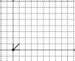
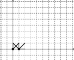
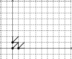
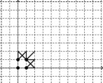
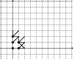
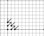
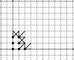
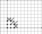
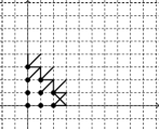
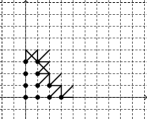
Figure 1. The unique (up to reflection in the line $y=x$) sequence of optimal nested sets for $1\leq|A|\leq 11$. The optimal nested set with $|A|=11$ has $|\partial A|=17$.

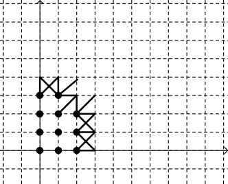
Figure 2. An optimal set having $|A|=11$ has $|\partial A|=16$. This set is better than the one of the same volume in Figure 1

Nested optimal sets are crucial for the technique of compression and the fact that the optimal sets are not nested means that such an approach will not be possible. However, as we will show, the monotonicity of the optimal boundary established here is a useful tool for obtaining bounds, proving optimality and understanding properties of optimal sets.

3. The Edge-Isoperimetric Problem in $(\mathbb{N}^{2},\infty)$

Given a set in ${{\mathbb{N}}}^{2}$, it can be made connected without increasing its volume by translating the connected components towards the origin. Moreover, it can be made to touch both axes. Call $A$ the resulting set. Let $X$ be the point on the $x$-axis with greatest $x$-coordinate and let $Y$ be the point on the $y$-axis of greatest $y$-coordinate. There is a connected subset $C$ of $A$ containing $X$ and $Y$. We argue that all points bounded by $C$ and the axes are in $A$ if $A$ is optimal.

Definition 4.

Given a connected subset $C$ of ${{\mathbb{N}}}^{2}$ containing at least one point on the $x$-axis and one point on the $y$-axis, we say that a point $z$ is bounded by $C$ if point $z$ is bounded by some piecewise linear curve formed by a subset of the edges of $C$ and the axes.

Lemma 5.

If $A$ is an optimal set, then it contains all lattice points bounded by the axes and a connected subset $C$ containing points $X$ and $Y$.

Proof.

Assume otherwise. Consider the subset $B_{C}\subset{{\mathbb{N}}}^{2}$ of points lying on or below $C$ and let $B=B_{C}\cup A$. Let $A_{C}=B_{C}\cap A$ be the points of $A$ lying on or below $C$. By assumption, $|B_{C}|>|A_{C}|$, so that $|B|>|A|$. We show that $|\partial B_{C}|<|\partial A_{C}|$. This implies that $|\partial B|<|\partial A|$, contradicting Theorem 2.
The perimeter $\partial B_{C}$ of $B_{C}$ consists not only of all edges of $C$ which lie outside of $B_{C}$, but also of the edges of the outermost layer of points of $B_{C}\setminus C$ (see Figure 3) if such points exist. In particular, a point $a\in B_{C}\setminus C$ contributes whenever the following conditions are met. Point $a$ is the vertex of a unit square $abcd$, the opposite corner $c$ is in the complement of $B_{C}$, and the other two corners $b$ and $d$ are on $C$. In this case, edge $ac$ is added to the perimeter. Suppose that such a point $a\in B_{C}\setminus A_{C}$ exists. Then the addition of $a$ to $A_{C}$ adds a diagonal edge $ac$ to the count but takes away the two edges $ab$ and $ad$. If $a$ is part of more than one square, it is easy to see that the perimeter will still be strictly improved. If $B_{C}\setminus A_{C}$ contains some point which does not meet the conditions, then it does not contribute to the perimeter of $B_{C}$. Since there is at least one point of this form or of the prior form, filling in these points strictly improves the perimeter. This completes the proof. $\Box$

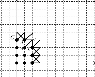
Figure 3. A connected subset $C$ containing $X$ and $Y$ is indicated by diamonds. The perimeter of the set bounded by $C$ receives a contribution not only from the points of $C$, but also from the layer adjacent to $C$, e.g., point $a$.

Conjecture 3.

For every volume, there is an optimal set $A$ which consists of the points bounded by a connected subset $C\subset A$ touching the axes.

We call sets consisting of the points bounded by a connected subset which touches the axes bounded. We will now investigate bounded sets. Though there might be sets which are better, we will still be able to learn much about the problem by considering bounded sets.

Definition 6.

Point $g\in{{\mathbb{Z}}}^{n}$ is a $j$-gap of a set $A$ if $g\notin A$ and there exists some point $p\in A$ with $p_{i}=g_{i}\mbox{ }\forall i\neq j$ and $g_{j}<p_{j}$.

We will say that a set has no gaps with it has no $j$-gaps for any $j=1,2,\ldots,n$.

Theorem 4.

For every volume, a bounded set can be modified to a bounded set with no gaps without increasing the boundary.

Proof.

We fill in the $1$-gaps starting from the lowest gaps by adding points such as $x$ in Figure 4, all the while decreasing the perimeter. By Theorem 2, the optimal perimeter is a monotonic increasing function of the volume, so we see that there can be no $1$-gaps. The same argument applies to the $2$-gaps. $\Box$

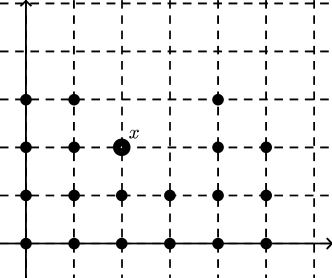
Figure 4. A bounded optimal set $A$ cannot have gaps since filling in the gap with points such as $x$ decreases the boundary.

Let $A_{t}=\{x\in A:x_{1}=t\}$.

Lemma 7.

A bounded optimal set can be chosen to have at most one $t\in\{1,2,...,k-1\}$ for which $|A_{t}|-|A_{t+1}|\geq 2$, and this $t$ can be chosen to be $k-1$.

Proof.

Let $t_{0}$ be the first $t$ for which $|A_{t}|-|A_{t+1}|\geq 2$ and assume that $t_{0}\neq k-1$. We can then transfer points from $A_{k}$ to $A_{t_{0}+1}$ until $|A_{t_{0}}|-|A_{t_{0}+1}|=1$ or $A_{k}$ has no more points left. Throughout, the perimeter does not increase because any point transferred shared at most $8$ edges with other points, and after the transfer shares at least $8$ edges. If $|A_{t_{0}}|-|A_{t_{0}+1}|$ is still greater than $2$, then we can transfer points from column $A_{k-1}$, and continue in this way until either $|A_{t_{0}}|-|A_{t_{0}+1}|=1$ or the number of columns has been reduced so that $t_{0}+1$ is the last column. $\Box$

Let us now view the heights of the columns as a function $h:\mathbb{N}\rightarrow\mathbb{N}$ given by $h(t)=|A_{t}|$. For brevity we will say that $h$ is constant whenever we mean that $h$ is constant on its support. We have already shown in Theorem 4 that a bounded optimal set exists which has $h$ non-increasing. We will show that $h$ can be made to take on a specific form. Before we do that, however, we note some special cases that are the only exceptions to the following Lemma. If $|A|=1$, $|A|=2$ or $|A|=4$, then it is easy to see that for the optimal set $h$ is constant. These are the only cases in which $h$ will be constant, as we show next.

Lemma 8.

Without increasing the boundary, a bounded set $A$ can be transformed into a bounded set $B$ for which $h_{B}$ is constant on $\{1,2,...,c-1\}$ and strictly decreasing on $\{c,c+1,...,k\}$. Moreover, if $|A|\neq 1,2,4$, we can choose $c<k$.

Proof.

Let $S=\{x,x+1,...,x+l\}$ be a maximal set of least $x$ for which $h(x+i)<h(x+i-1)\mbox{ }\forall i=1,...,l$. Assume further that $x+l<k$. We consider two cases: when $x+l=k-1$ and when $x+l<k-1$. In the former case, we take the top point from column $A_{k}$, which has at most $6$ shared edges, and place it on top of column $A_{k-1}$, and now it has at least $6$ shared edges. This reduces us to the second case. In this case, we take a point from column $A_{k}$, which can have at most $8$ shared edges, and place it at the top of column $A_{x+l}$. Because $h(x+l)=h(x+l+1)$ and $h(x+l-1)=h(x+l)+1$, the new point has $8$ shared edges, so the perimeter is not increased. We have now reduced $S$ to $S\setminus\{x+l\}$, and we continue inductively. This shows that $A$ can be transformed into a set $B$ for which $h_{B}$ is constant on $\{1,2,...,c-1\}$ and strictly decreasing on $\{c,c+1,...,k\}$.

To see that we can choose $c<k$, assume that $|A|\neq 1,2,4$ and that $h$ is constant. If $k=1$, then we can take the top point of $A_{k}$ and place it at $A_{2}$ without increasing the perimeter. If $k=2$, we can take the point $P$ at the top of $A_{k}$ and place it at $A_{k+1}$. Since $h_{A}$ was constant, $P$ had at most $3$ neighbours. Placing $P$ at $A_{k+1}$ guarantees $2$ neighbours and $3$ boundary edges, so the perimeter is not increased. For $k\geq 3$, we can take the point $P$ from the top of $A_{k}$ and place it at the top of $A_{1}$, and because $k\geq 3$, $P$ will not have $2$ neighbours and $3$ boundary edges. $\Box$

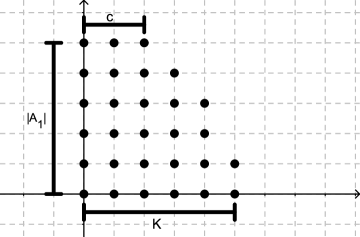
Figure 5. Schematic depicting the form of an optimal bounded set guaranteed by Lemmas 7 and 8. The first $c$ columns have the same height $|A_{1}|$, the next $k-c-1$ columns have heights decreasing by $1$ at each step, and the last column $A_{k}$ has height $|A_{k}|$ less than $|A_{k-1}|$.

We can now find the perimeter of a general set subject to the conditions in the Lemmas above in terms of $|A_{1}|$, $|A_{k}|$, $k$ and $c$. There are $|A_{1}|$ horizontal edges and $k$ vertical edges. There are $\sum_{t=1}^{k-1}(|A_{t}|-|A_{t+1}|+1)+|A_{k}|=|A_{1}|+k-1$ edges parallel to $e_{1}+e_{2}$, $|A_{k}|-1+\max\{|A_{k-1}|-|A_{k}|-1,0\}=|A_{k}|-1+|A_{k-1}|-|A_{k}|-1=|A_{k-1}|-2$ edges in the $e_{1}-e_{2}$ direction, and $\sum_{t=2}^{k}\delta_{|A_{t}|,|A_{t-1}|}=c-1$ edges in the direction $e_{2}-e_{1}$. Consequently, the perimeter is $2|A_{1}|+|A_{k-1}|+c+2k-4=2|A_{1}|+|A_{1}|-(k-1-c)+c+2k-4$, which is equal to

(1) $$|\partial A|=3|A_{1}|+2c+k-3.$$

We also know that $\sum_{t=1}^{k}|A_{t}|=|A|$. Therefore $|A|=c|A_{1}|+\sum_{i=1}^{k-c-1}(|A_{1}|-i)+|A_{k}|,$ which simplifies to

(2) $$|A|=(k-1)|A_{1}|+|A_{k}|-\frac{(k-c-1)(k-c)}{2}.$$

Combining Theorem 2 on the monotonicity of the perimeter and equation 1, we obtain:

Corollary 9.

Let $A$ be a bounded optimal set with $|A_{k}|<|A_{k-1}|-1$. Then the optimal perimeter of bounded sets of cardinality $|A|+1$ is $|\partial A|$ and a bounded optimal set of cardinality $|A|+1$ is given by $A\cup\{(k,|A_{k}|+1)\}$.

Example 10.

We show that simplices are not always optimal. Consider the simplex given by $h_{i}=15-i$, $i=1,2,...,14$. By increasing $|A_{1}|$ by $1$ while preserving the shape from Lemma 8, we get a truncated simplex given by $h_{i}=16-i$, $i=1,2,...,10$. The perimeter of the simplex is $56$, whereas that of the truncated simplex is $55$.

Given $|A_{1}|$, $c$ and $|A|$, the set $A$ is determined. Indeed, we know that

$$|A_{i}|=\begin{cases}|A_{1}|&i\leq c\\ |A_{1}|-i+c&c+1\leq i\leq k-1\\ |A|+\frac{(k-c-1)(k-c)}{2}-(k-1)|A_{1}|&i=k\end{cases}$$

Moreover, $k$ is the unique positive integer such that

$$\sum_{i=1}^{k-c-1}(|A_{1}|-i)<|A|-c|A_{1}|\leq\sum_{i=1}^{k-c}(|A_{1}|-i).$$

Solving for $k$, we obtain

$$k=\lceil\frac{1}{2}(-1+2|A_{1}|-\sqrt{1+8(\binom{|A_{1}|}{2}-|A|+c|A_{1}|)}\rceil+c.$$

Therefore the problem is to minimize

$$|\partial A|=3|A_{1}|+3c+\lceil\frac{1}{2}(-1+2|A_{1}|-\sqrt{1+8(\binom{|A_{1}|}{2}-|A|+c|A_{1}|)})\rceil-3$$

$$=4|A_{1}|+3c-3-\lfloor\frac{1}{2}(1+\sqrt{1+8(\binom{|A_{1}|}{2}-|A|+c|A_{1}|)})\rfloor.$$

Lemma 11.

Any bounded set $A$ can be transformed into one for which $|A_{1}|\geq c$ without increasing the boundary.

Proof.

Assume that $|A_{1}|<c$. We reflect $A$ in the line $y=x$ to obtain a new set $B$ which has $|A_{1}|$ columns. The first $|A_{k}|$ are of height $k$. Columns $|A_{k}|+1$ through $|A_{k-1}|$ are of height $k-1$. The remaining columns decreased in height by steps of $1$, with column $|A_{k-1}|+1$ having height $k-2$ and column $|A_{1}|$ having height $c$. Since $c>|A_{1}|>|A_{k-1}|-|A_{k}|$, we can take points from column $|A_{1}|$ of height $c$ and place them on top of columns $|A_{k}|+1$,…,$|A_{k-1}|-1$ without increasing the perimeter. The resulting set has the form of Lemma 8. The new parameters are $\tilde{|A_{1}|}=k$, $\tilde{k}=|A_{1}|$ and $\tilde{c}=|A_{k-1}|-1=|A_{1}|-k+c$. Then

$$c>|A_{1}|\implies\tilde{c}=|A_{1}|-k+c<2c-k.$$

Since $k>c$, $|\tilde{A_{1}}|>\tilde{c}.$ $\Box$

In order to obtain a lower bound for the sets considered, we relax our problem to a continuous one:

$$\underset{|A_{1}|,c\in\mathbb{R}}{\text{minimize}} 4|A_{1}|+3c-3-\frac{1}{2}(1+\sqrt{1+8(\binom{|A_{1}|}{2}-|A|+c|A_{1}|)})$$

subject to $$1\leq|A_{1}|\leq|A|,$$

$$\frac{|A|-\binom{|A_{1}|}{2}}{|A_{1}|}\leq c\leq|A_{1}|.\;$$

For any $|A|\geq 2$, we can establish via a direct calculation that the minimum value of the objective is $\sqrt{\frac{7}{2}}\sqrt{8|A|-1}-2$ given by the unconstrained minimizer $|A_{1}|=\frac{3\sqrt{8|A|-1}}{2\sqrt{14}}$ and $c=\frac{1}{28}(14+\sqrt{14}\sqrt{8|A|-1})$, and the value is better than the value of the function on the boundary of the feasible region.

To obtain an upper bound, we will utilize the monotonicity of the perimeter from Theorem 2. Let $m\in\mathbb{N}$ and set $|A|^{*}=7m^{2}$, $|A_{1}|^{*}=3m$ and $c^{*}=m$. It is again a simple calculation to verify that these values give a feasible point. The function

$$g(|A_{1}|,c)=4|A_{1}|+3c-2-\frac{1}{2}(1+\sqrt{1+8(\binom{|A_{1}|}{2}-|A|+c|A_{1}|)})$$

is an upper bound for the perimeter. For $|A|^{*}=7m^{2}$,

$$g(|A_{1}|^{*},c^{*})=15m-\frac{1}{2}\sqrt{4m^{2}-12m+1}-\frac{5}{2}$$

$$=\frac{15}{\sqrt{7}}\sqrt{|A|^{*}}-\frac{1}{2}\sqrt{\frac{4}{7}|A|^{*}-\frac{12}{\sqrt{7}}\sqrt{|A|^{*}}+1}.$$

For a general $|A|$, we find $m$ such that $7(m-1)^{2}<|A|\leq 7m^{2}$. Then $|A|^{*}\leq|A|+2\sqrt{7|A|}-8$, so that

$$|\partial A|\leq\frac{15}{\sqrt{7}}\sqrt{|A|+2\sqrt{7|A|}-8}-\frac{1}{2}\sqrt{\frac{4}{7}(|A|+2\sqrt{7|A|}-8)-\frac{12}{\sqrt{7}}\sqrt{|A|+2\sqrt{7|A|}-8}+1}.$$

This complicated expression is asymptotically

$$\frac{15}{\sqrt{7}}\sqrt{|A|}-\frac{1}{\sqrt{7}}\sqrt{|A|}=\sqrt{\frac{7}{2}}\sqrt{8|A|}.$$

Note, however, that the upper bound is real if and only if $|A|\geq 36$.

Theorem 5.

Let the cardinality of a bounded optimal set $A$ be $|A|\geq 36$. Then the perimeter $|\partial A|$ is bounded below by

$$\lceil\sqrt{\frac{7}{2}}\sqrt{8|A|-1}-2\rceil$$

and above by

$$\lfloor\frac{15}{\sqrt{7}}\sqrt{|A|+2\sqrt{7|A|}-8}-\frac{1}{2}\sqrt{\frac{4}{7}(|A|+2\sqrt{7|A|}-8)-\frac{12}{\sqrt{7}}\sqrt{|A|+2\sqrt{7|A|}-8}+1}\rfloor.$$

Moreover, the difference between the upper and lower bound does not exceed the constant $\frac{35}{2}$.

Proof.

The upper and lower bounds were shown above. Rather than consider the upper bound as it stands, we consider the slightly weaker but simpler upper bound $u(|A|)$ equal to

$$\frac{15}{\sqrt{7}}\sqrt{|A|+2\sqrt{7|A|}-8}-\frac{1}{2}\sqrt{\frac{4}{7}(|A|+2\sqrt{7|A|}-8)-\frac{12}{\sqrt{7}}\sqrt{|A|+2\sqrt{7|A|}-8}}$$

obtained by dropping the $1$ inside of the square root. Then a calculation shows that the difference $d(|A|)$ between the upper bound $u(|A|)$ and lower bound $l(|A|)=\sqrt{\frac{7}{2}}\sqrt{8|A|-1}-2$ has a non-vanishing derivative. Moreover, at $|A|=39$, the first point at which this upper bound is defined, the derivative of the difference is positive, so that the difference is an increasing function. Taking the limit, we obtain the value $\frac{35}{2}$. For any $36\leq|A|\leq 38$, a direct calculation shows that the difference is at most $\frac{35}{2}$. $\Box$

Note that the growth of the boundary, even for bounded optimal sets, is slower than linear, though by Theorem 2 the perimeter is an increasing function. Therefore

Corollary 12.

There exist arbitrarily long consecutive values of the volume for which the minimum boundary is the same.

4. Acknowledgements

I would like to thank Professor Simon Brendle for his helpful suggestions throughout the writing of this note.

References

- [1] Wang, D.-L. and Wang, P. (1977) Discrete isoperimetric problems. SIAM J. Appl. Math. 32 860-870.
- [2] Béla Bollobás and Imre Leader. Edge-isoperimetric inequalities in the grid. Combinatorica, 11(4):299-314, 1991.
- [3] E. Veomett, A. J. Radcliffe.Vertex Isoperimetric Inequalities for a Family of Graphs on . The Electronic Journal of Combinatorics 19(2) (2012), #P45.