Margins, Shrinkage, and Boosting

Abstract

This manuscript shows that AdaBoost and its immediate variants can produce approximate maximum margin classifiers simply by scaling step size choices with a fixed small constant. In this way, when the unscaled step size is an optimal choice, these results provide guarantees for Friedman’s empirically successful “shrinkage” procedure for gradient boosting (Friedman, 2000). Guarantees are also provided for a variety of other step sizes, affirming the intuition that increasingly regularized line searches provide improved margin guarantees. The results hold for the exponential loss and similar losses, most notably the logistic loss.

1 Introduction

AdaBoost and related boosting algorithms greedily aggregate many simple predictors into a single accurate predictor (Freund & Schapire, 1997). One explanation for the efficacy of boosting is that it not only seeks aggregates with low empirical risk, but moreover that it prefers good margins, which leads to improved generalization (Schapire et al., 1997). Since AdaBoost does not attain maximum margins on general instances, a push was made to develop methods which carry such a guarantee (Rätsch & Warmuth, 2005; Shalev-Shwartz & Singer, 2008; Rudin et al., 2007).

This work shows that margin maximization may be achieved by scaling back the step size. The intuition for this result is simple (cf. Figure 1): when (equivalently) considered as steps in a coordinate descent procedure, the iterates, depicted as a path, approximate the path of constrained optima (for all possible choices of constraint). By scaling back the step size, the optimal path is more finely approximated. As there have been many proposed step sizes for these methods, this manuscript will study four separate choices, deriving improved bounds for the more regularized choices. While it has been shown before that regularized step sizes have good generalization and asymptotically good margins (Zhang & Yu, 2005), this manuscript shows that straightforward step choices achieve these margins at rates matching explicitly margin-maximizing boosting methods.

This practice of scaling back weights was proposed by Friedman (2000, Section 5), who referred to it as a shrinkage scheme (Copas, 1983). This scheme is effective, and adopted in practice (see for instance Bradski (2000, Class CvGBTrees) and Pedregosa et al. (2011, Class GradientBoostingClassifier)); the purpose of this manuscript is to provide theoretical guarantees.

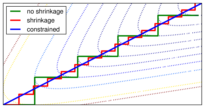
Figure 1: The blue diagonal line is the empirical risk minimizer subject to varying $l^{1}$ constraints, and is also a maximum margin choice. The green line takes optimal steps, and grossly overshoots the optimal path. By applying mild shrinkage, the red line approximates the maximum margin choice much more finely.

1.1 Outline

After summarizing the main content, this introduction closes with connections to related work; thereafter, Section 2 recalls the core algorithm, defines the class of loss functions, and provides the four step sizes.

As boosting is generally studied under the weak learning assumption (a separability condition), the dominant study in this manuscript is also under the condition of separability, and appears in Section 3. The first step is to show that shrinkage does not drastically change the rate of convergence of the empirical risk under these methods. The more involved study is on the topic of margins, and the final subsection compares these bounds to those of other methods.

General (potentially nonseparable) instances are discussed in Section 4. Once again, the first step is a convergence rate guarantee, which again matches those without shrinkage. This section also demonstrates that, under a certain decomposition of boosting problems, the algorithm is still achieving margins on a separable sub-component of the problem.

The manuscript closes with some discussion in Section 5. All proofs are relegated to appendices (in the supplementary material).

1.2 Related Work

Three close works proposed regularized line searches for boosting. First, Friedman (2000) gave the same scheme as is considered here (albeit with only the optimal line search); follow-up work has been mainly empirical, and the questions of convergence rates and margin guarantees do not appear in the literature. Second, Zhang & Yu (2005) also considered regularized line searches, but with a goal of proving consistency; margin maximization is proved as a byproduct, and the analogous results here hold under fewer conditions, and come with rates for the more stringent step sizes. A third work, due to Rätsch et al. (2001), also proves margin maximizing properties of regularized line searches, but again without rates.

As mentioned in the introduction, margin maximization properties of AdaBoost have received extensive study; an excellent survey of results with pointers to other literature is provided by Schapire & Freund (2012, Chapter 5). Amongst these, a crucial result, due to Rudin et al. (2004), provides a concrete input to AdaBoost which yields suboptimal margins (which is used in Section 3.3); that work also studies the evolution of these margins as a dynamical system, a topic which will reappear in Section 5.

The primary contribution of this manuscript is to exhibit margin maximization, thus a natural comparison is to other algorithms with this same guarantee, for instance the works of Rätsch & Warmuth (2005), Shalev-Shwartz & Singer (2008), and Rudin et al. (2007) (or again refer to Schapire & Freund (2012, Chapter 5, Bibliographic Notes) for a more extensive summary). This manuscript will briefly compare with the methods of Shalev-Shwartz & Singer (2008), which subsume some earlier results and match the best guarantees, along with giving a simple, general, greedy scheme. The key distinction between previous work and the present work is firstly that the algorithmic modifications here are minor (in particular, the form of unregularized empirical risk minimization is unchanged), and that properties of an existing, widely used method are discerned (namely, the shrinkage procedure presented by Friedman (2000)).

As is standard in the above works, this manuscript is only concerned with convergence of empirical quantities.

In order to prove convergence rates, this work relies heavily on techniques due to Telgarsky (2012). In particular, the scheme to prove convergence rates of empirical risk, detailed properties of splitting out a hard core from a boosting instance (cf. Section 4), and the notion of relative curvature (cf. Section 2.1) are all due to Telgarsky (2012). The intent of the present manuscript is to establish margin properties, and in this regard it departs from Telgarsky (2012); by contrast, the convergence rates of empirical risk presented here are thus trivial, but included since they did not appear explicitly in the literature. It is worth mentioning that these methods produce bad constants when applied to the logistic loss; unfortunately, previous work also suffers in this case (for instance, the work of Collins et al. (2002) provided only convergence of empirical risk, and not rates).

2 Algorithms and Notation

First some basic notation. Let $\{(x_{i},y_{i})\}_{i=1}^{m}\subseteq\mathcal{X}\times\{-1,+1\}$ denote an $m$-point sample. Take $\mathcal{H}_{0}$ to denote the collection of weak learners; it is assumed that $h\in\mathcal{H}_{0}$ satisfies $h(\mathcal{X})\subseteq[-1,+1]$, and that $\mathcal{H}_{0}$ has some form of bounded complexity, meaning specifically that the set of vectors $\{(h(x_{1}),\ldots,h(x_{m})):h\in\mathcal{H}_{0}\}$ is finite; this for instance holds if there is a fixed finite set of outputs from $\mathcal{H}_{0}$, e.g., each $h$ is binary. Consequently, let $\mathcal{H}=\{h_{j}\}_{j=1}^{n}$ denote the effective finite set of hypothesis, and collect the responses on the sample into a matrix $A\in[-1,+1]^{m\times n}$ with $A_{ij}=-y_{i}h_{j}(x_{i})$.

Boosting finds a weighting $\lambda\in\mathbb{R}^{n}$ of $\mathcal{H}$, which corresponds to a regressor $x\mapsto\sum_{j=1}^{n}\lambda_{j}h_{j}(x)$, and thus a binary classification rule after thresholding. The corresponding ($l_{1}$ minimum) margin $\mathcal{M}(A\lambda)$ over the sample with respect to $\lambda$ is

$$\mathcal{M}(A\lambda):=\min_{i\in[m]}\frac{-\textbf{e}_{i}^{\top}A\lambda}{\|\lambda\|_{1}}=\min_{i\in[m]}\frac{y_{i}\sum_{j=1}^{n}\lambda_{j}h_{j}(x_{i})}{\|\lambda\|_{1}}.$$

Let $\gamma$ denote the best (largest) achievable margin; equivalently (Shalev-Shwartz & Singer, 2008), $\gamma$ is the weak learning rate (which justifies the choice of $l_{1}$ margins):

$$\gamma :=\max_{\begin{subarray}{c}\lambda\in\mathbb{R}^{n}\\ \|\lambda\|_{1}=1\end{subarray}}\mathcal{M}(A\lambda)=\max_{\begin{subarray}{c}\lambda\in\mathbb{R}^{n}\\ \|\lambda\|_{1}=1\end{subarray}}\min_{i\in[m]}-\textbf{e}_{i}^{\top}A\lambda$$

$$=\min_{w\in\Delta_{m}}\max_{j\in[n]}\left|\sum_{i=1}^{m}w_{i}y_{i}h_{j}(x_{i})\right|=\min_{w\in\Delta_{m}}\|A^{\top}w\|_{\infty}.$$

When $\gamma>0$, the instance is considered separable; classically, this condition is termed the weak learning assumption (Kearns & Valiant, 1989; Freund & Schapire, 1997).

2.1 The Family of Loss Functions

The class $\mathbb{L}$ will effectively be “functions similar to the exponential loss”. Some of this is for analytic convenience, but some of this appears to be essential, and thus a bit of motivation is appropriate.

Optimization problems typically take advantage of curvature (e.g., strong convexity) to establish a convergence rate. The analysis here instead uses a relative form of curvature: it suffices for, say, the Hessian to not be too small relative to the gap between the current primal objective value and the primal optimum. In this sense, the exponential loss is ideal, as it is a fixed point of the differentiation operator.

Definition 2.0.

Given a loss $\ell:\mathbb{R}\to\mathbb{R}_{++}$ (where $\mathbb{R}_{++}$ denotes positive reals), let $C_{\ell}(z)\geq 1$ (with potentially $C_{\ell}(z)=\infty$) be the tightest positive constant so that, for every $x\leq z$: $C_{\ell}(z)^{-1}\leq\exp(x)/\ell^{(i)}(x)\leq C_{\ell}(z)$ for $i\in\{0,1,2\}$ (the zeroth, first, and second derivatives).

Since $C_{\ell}(z)$ is defined to be the tightest constant, it follows that $y\leq z$ implies $C_{\ell}(y)\leq C_{\ell}(z)$.

From here, the class of loss functions may be defined.

Definition 2.0.

Let $\mathbb{L}$ contain all functions $\ell:\mathbb{R}\to\mathbb{R}_{+}$ which are twice continuously differentiable, strictly convex, and have $C_{\ell}(z)<\infty$ for all $z\in\mathbb{R}$. Additionally, if $\lim_{z\to-\infty}C_{\ell}(z)=1$, then $\ell\in\mathbb{L}_{\infty}$.

Crucially, the two classes $\mathbb{L}$ and $\mathbb{L}_{\infty}$ both contain the exponential and logistic losses.

Proposition 2.0.

$\{x\mapsto\exp(x),x\mapsto\ln(1+\exp(x))\}\subseteq\mathbb{L}_{\infty}$.

One way to interpret this is to say “in the limit, logistic loss is the same as exponential loss”. Unfortunately, this treatment of the logistic loss ends up being quite unfair, in the sense that the bounds are not accurately representative of the behavior of the algorithm (see Section 3.3). It is, however, unclear how to better deal with the logistic loss.

Lastly, the relevant primal objective function may be defined.

Definition 2.0.

Given $\ell\in\mathbb{L}$ and vector $z\in\mathbb{R}^{m}$, define $\mathcal{L}(z):=m^{-1}\sum_{i=1}^{m}\ell(z_{i})$, whereby the primal optimization problem for boosting is to minimize $\mathcal{L}(A\lambda)$ over the domain $\mathbb{R}^{n}$. For convenience, define $\bar{\mathcal{L}}_{A}:=\inf_{\lambda\in\mathbb{R}^{n}}\mathcal{L}(A\lambda)$.

2.2 Algorithm

The algorithm appears in Algorithm 1. Before defining the various step sizes, two more definitions are in order.

Algorithm 1 $\textsc{boost}.$
Input: loss $\ell$, matrix $A\in[-1,+1]^{m\times n}$.
Output: Weighting sequence $\{\lambda_{t}\}_{t=0}^{\infty}$.

  Initialize $\lambda_{0}:=0$.

  for $t=1,2,\ldots:$ do

     Choose column (weak learner)

$$j_{t}:=\operatornamewithlimits{arg\,max}_{j}|\nabla\mathcal{L}(A\lambda_{t-1})^{\top}A\textbf{e}_{j}|.$$

     Set descent direction $v_{t}\in\{\pm\textbf{e}_{j_{t}}\}$, whereby

$$\nabla\mathcal{L}(A\lambda_{t-1})^{\top}Av_{t}=-\|\nabla\mathcal{L}(A\lambda_{t-1})^{\top}A\|_{\infty}.$$

     Find $\alpha_{t}$ via line search.

     Update $\lambda_{t}:=\lambda_{t-1}+\alpha_{t}v_{t}$.

  end for

Definition 2.0.

For every $t$, define $\gamma_{t}:=\|A^{\top}\nabla\mathcal{L}(A\lambda_{t-1})\|_{\infty}/\|\nabla\mathcal{L}(A\lambda_{t-1})\|_{1}$. (Note that $1\geq\gamma_{t}\geq\gamma$.)

Additionally, rather than depending on parameter $C_{\ell}(z)$ for a carefully chosen $z$, the following definition suffices.

Definition 2.0.

For $t\geq 1$, define $C_{t}:=C_{\ell}(\ell^{-1}(m\mathcal{L}(A\lambda_{t-1})))$.

The significance of $C_{t}$ is as follows. Since the algorithm itself is coordinate descent, and moreover since every line search will be shown to guarantee descent, every candidate $\lambda$ considered in round $t$ will satisfy $\mathcal{L}(A\lambda)\leq\mathcal{L}(A\lambda_{t-1})$; thus, for every $i\in[m]$, $\ell(\textbf{e}_{i}^{\top}A\lambda)\leq m\mathcal{L}(A\lambda)\leq m\mathcal{L}(A\lambda_{t-1})$, and so $\textbf{e}_{i}^{\top}A\lambda\leq\ell^{-1}(m\mathcal{L}(A\lambda_{t-1}))$, where the inverse is well-defined since $\ell$ is a bijection between $\mathbb{R}$ and $\mathbb{R}_{++}$ by definition of $\mathbb{L}$ (otherwise $C_{\ell}(z)=\infty$).

The collection of step sizes considered here are as follows, in order of least to most aggressive. Throughout these step sizes, $\nu\in(0,1]$ will denote a shrinkage parameter.

Quadratic upper bound.

Rather than performing an optimal line search, i.e., rather than minimizing $\alpha\mapsto\mathcal{L}(A(\lambda_{t-1}+\alpha v_{t}))$, a quadratic upper bound of this univariate function may be minimized, which has a closed form solution (cf. the proof of Section 3.1). In particular, define the step size $\alpha_{t}^{\textup{Q}}(\nu):=\nu\gamma_{t}/C_{t}^{4}$. This choice is pleasant algorithmically only when $C_{t}$ is easy to compute (for instance, $C_{t}=1$ for the exponential loss). In general, however, it is useful as an analytic aid, since most step sizes here can be lower bounded by it. This step size was introduced by Telgarsky (2012, Appendix D.3).

Wolfe.

The Wolfe line search is a standard tool from nonlinear optimization (Nocedal & Wright, 2006, chapter 3), and for convex problems it may be implemented with binary search (Telgarsky, 2012, Appendix D.1). More precisely, this choice is a set of step sizes $\alpha_{t}^{\textup{W}}(\nu)$ satisfying two conditions. First, the step is explicitly disallowed from being too large:

$$\mathcal{L}(A(\lambda_{t-1}+\alpha v_{t}))$$

$$\quad\leq\mathcal{L}(A\lambda_{t-1})-\alpha(1-\nu/2)\|A^{\top}\nabla\mathcal{L}(A\lambda_{t-1})\|_{\infty}.$$ (2.1)

Second, the step should be approximately optimal (in terms of the line search problem):

$$\nabla\mathcal{L}(A(\lambda_{t-1}+\alpha v_{t}))^{\top}Av_{t}$$

$$\quad\geq-(1-\nu/4)\|\nabla\mathcal{L}(A\lambda_{t-1})^{\top}A\|_{\infty}.$$ (2.2)

(Requiring the reverse inequality (with the right hand side negated) yields the Strong Wolfe Conditions, which are not necessary here.) In contrast to $\alpha_{t}^{\textup{Q}}(\nu)$, the Wolfe step does not require knowledge of $C_{t}$, but will yield nearly identical bounds; in fact, computation of the Wolfe step requires only function evaluations, gradient evaluations, and knowledge of $\nu$, $A$,$v_{t}$, $\lambda_{t}$.

AdaBoost.

Following the scheme of AdaBoost, define $\alpha_{t}^{\textup{A}}(\nu):=\frac{\nu}{2}\ln(\frac{1+\gamma_{t}}{1-\gamma_{t}})$, where convention is followed and $\gamma_{t}=1$ is ignored. Unfortunately, even though $\gamma_{t}$ is loss-dependent, this step will only yield rates with the exponential loss. However, it will be instrumental in analyzing the fully optimizing step size, presented next. This step size was introduced with the original presentation of AdaBoost (Freund & Schapire, 1997), though the analysis here will rather follow a slightly later treatment (Schapire & Singer, 1999).

Optimal.

Let $\alpha_{t}^{\textup{O}}(1)$ be a minimizer to $\alpha\mapsto\mathcal{L}(A(\lambda_{t-1}+\alpha v_{t}))$, which, as in the case of $\alpha_{t}^{\textup{A}}(\nu)$, is assumed to exist. For $\nu\in(0,1)$, set $\alpha_{t}^{\textup{O}}(\nu)=\nu\alpha_{t}^{\textup{O}}(1)$. When $A$ is binary and $\ell=\exp$, $\alpha_{t}^{\textup{O}}(\nu)=\alpha_{t}^{\textup{A}}(\nu)$, though in general this is not true. This step size (with shrinkage!) was suggested by Friedman (2000) for use with the logistic loss.

To close, note that $\alpha_{t}^{\textup{Q}}(\nu)$ and $\alpha_{t}^{\textup{O}}(\nu)$ have a simple relationship.

Proposition 2.2.

If $A\in[-1,+1]^{m\times n}$ and $\ell\in\mathbb{L}$, then $\alpha_{t}^{\textup{Q}}(\nu)\leq\alpha_{t}^{\textup{O}}(\nu)$.

3 The Separable Case

This section considers the setting of separability, meaning the weak learning assumption is satisfied ($\gamma>0$). The three subsections respectively provide convergence rates in empirical risk, basic margin guarantees, and close with some discussion.

3.1 Convergence of Empirical Risk

The basic guarantee is that all of these line search methods, for any loss in $\mathbb{L}$ and with arbitrary shrinkage, exhibit the same basic convergence rate as AdaBoost.

Theorem 3.1.

Let boosting matrix $A$ with corresponding $\gamma>0$ and shrinkage parameter $\nu\in(0,1]$ be given. Given any $\ell\in\mathbb{L}$, any $\epsilon>0$, and iterates $\{\lambda_{t}\}_{t\geq 0}$ consistent with $\alpha_{t}^{\textup{Q}}(\nu)$, $\alpha_{t}^{\textup{W}}(\nu)$, $\alpha_{t}^{\textup{O}}(\nu)$, or $\alpha_{t}^{\textup{A}}(\nu)$ with $\ell=\exp$, then $\mathcal{O}(\frac{1}{\gamma^{2}}\ln(\frac{1}{\epsilon}))$ iterations suffice to ensure $\mathcal{L}(A\lambda_{t})\leq\epsilon$, where the $\mathcal{O}(\cdot)$ suppresses terms depending on $C_{1}$ and $\nu$.

The proof is in the appendix, but a basic discussion will appear here for each step size. The proofs are straightforward, as they should be: convergence analyses typically prove a bound for one step, and then iterate the bound. As such, taking $1/\nu$ steps which are $\nu$-factor as long as the original should do at least as well as the original (which is indeed the exhibited trade-off).

First is the quadratic upper bound, which implicitly gives an upper bound for the optimal step as well. The proof follows a standard scheme from convex optimization of lower and upper bounding a potential function based on the gradient; the specifics use the relative curvature properties of $\mathbb{L}$, and follow the analysis of Telgarsky (2012, Section 6.1, Appendix D).

Lemma 3.1.

Consider the setting of Theorem 3.1, but with each step size $\alpha_{t}$ satisfying $\alpha_{t}^{\textup{Q}}(\nu)\leq\alpha_{t}\leq\alpha_{t}^{\textup{O}}(\nu)$. Then for any $t>t_{0}\geq 0$,

$$\mathcal{L}(A\lambda_{t})\leq\mathcal{L}(A\lambda_{t_{0}})\exp\left(-\frac{\nu(2-\nu)}{2C_{t_{0}+1}^{6}}\sum_{i=t_{0}+1}^{t}\gamma_{i}^{2}\right).$$

The reason for the parameter $t_{0}$ is to mitigate the horrendous dependence on $C_{t_{0}}$, which is potentially very large. In particular, consider $\ell\in\mathbb{L}_{\infty}$, meaning $\lim_{z\to-\infty}C_{\ell}(z)=1$. $C_{1}$ may be quite bad, but convergence still happens. It follows that $C_{t}\to 1$, and thus, by choosing some large $t_{0}$, the bound provides that perhaps there is an initially slow convergence phase, but eventually it is very fast. That is to stay, Section 3.1 may be applied multiple times to give a more refined picture of the convergence, particularly in the case that $\ell\in\mathbb{L}_{\infty}$, which guarantees the constants are eventually near 1.

Next, the Wolfe step size has a similar guarantee (and the analysis once again heavily relies on techniques due to Telgarsky (2012, 6.1, Appendix D)).

Lemma 3.1.

Consider the setting of Theorem 3.1, but with $\alpha_{t}\in\alpha_{t}^{\textup{W}}(\nu)$. Then for any $t>t_{0}\geq 0$,

$$\mathcal{L}(A\lambda_{t})\leq\mathcal{L}(A\lambda_{t_{0}})\exp\left(-\frac{\nu(2-\nu)}{8C_{t_{0}+1}^{6}}\sum_{i=t_{0}+1}^{t}\gamma_{i}^{2}\right).$$

(The denominator blows up by a factor 4 due to extra halves introduced into the Wolfe conditions, specifically to adjust around the natural Wolfe parameters being within $(0,1)$ and not $(0,1]$.)

Lastly, consider $\alpha_{t}^{\textup{A}}(\nu)$. As in the statement of Theorem 3.1, this step size is only shown to work with the exponential loss. This may be an artifact of the analysis, however, which perhaps follows too closely the treatment of Schapire & Singer (1999), which only considers the exponential loss; for instance, a slightly modified step size can be used to show convergence with the logistic loss (Collins et al., 2002).

Lemma 3.1.

Consider the setting of Theorem 3.1, but with $\alpha_{t}\in\alpha_{t}^{\textup{A}}(\nu)$ Then for any $t>t_{0}\geq 0$,

$$\mathcal{L}(A\lambda_{t})\leq\mathcal{L}(A\lambda_{t_{0}})\prod_{i=t_{0}+1}^{t}C_{i}^{3}\left(1-\frac{\nu}{2}\gamma_{i}^{2}\right).$$

3.2 Margin Maximization

The margin rates here follow a simple pattern: the more regularized the step size, the faster the convergence to a good margin. While no lower bounds are presented, this is an interesting and intuitive correspondence (in particular, consistent with Figure 1). Unfortunately, the unconstrained step sizes only have asymptotic convergence (no rates), so the umbrella theorem for this subsection is also asymptotic.

Theorem 3.2.

Let boosting matrix $A$ with corresponding $\gamma>0$ and shrinkage parameter $\nu\in(0,1]$ be given. Given any $\ell\in\mathbb{L}_{\infty}$, any $\epsilon>0$, and iterates $\{\lambda_{t}\}_{t\geq 0}$ consistent with $\alpha_{t}^{\textup{Q}}(\nu)$, $\alpha_{t}^{\textup{W}}(\nu)$, $\alpha_{t}^{\textup{A}}(\nu)$ with $\ell=\exp$, or $\alpha_{t}^{\textup{O}}(\nu)$ with binary $A\in\{-1,+1\}^{m\times n}$, then there exists $T$ so that for all $\mathcal{M}(A\lambda_{t})\geq\gamma-\epsilon$ for all $t\geq T$.

In contrast with the convergence rates of empirical risk (e.g., Theorem 3.1), the condition $\ell\in\mathbb{L}_{\infty}$ is made, rather than simply $\ell\in\mathbb{L}$ (with improved constants when $\ell\in\mathbb{L}_{\infty})$. This can be interpreted to say: the analysis depends heavily upon the structure of the exponential loss. While this condition is likely unnecessary, on the other extreme it is important for the loss to be strictly convex; if for instance the hinge loss is used, then minimization can stop at any point achieving zero error, in particular at one with poor margin properties.

Returning to task, the quadratic upper bound comes first.

Lemma 3.2.

Suppose the setting of Theorem 3.2, but with $\alpha_{t}=\alpha_{t}^{\textup{Q}}(\nu)$. Additionally let $t>t_{0}\geq 0$ be given with $t\geq\frac{2C_{1}^{6}\ln(m)}{\gamma^{2}\nu(2-\nu)}$ (whereby all margins are nonnegative by Section 3.1). Then

$$\mathcal{M}(A\lambda_{t}) \geq\gamma\left(\frac{2-\nu}{2C_{t_{0}+1}^{6}}\right)-\frac{\ln(c_{0})}{t\nu\gamma},$$

where

$$c_{0}\!:=\!\max\!\left\{\!1,mC_{t_{0}+1}\mathcal{L}(A\lambda_{t_{0}})\exp\left(\frac{\nu(2-\nu)}{2C_{t_{0}+1}^{6}}\sum_{i=1}^{t_{0}}\gamma_{i}^{2}\right)\!\!\right\}\!.$$

To interpret this bound, first consider the simplifying case that $\ell=\exp$, whereby $C_{t}=1$ for all $t$. Additionally taking $t_{0}=0$, it follows that $c_{0}=m$, and the bound is simply

$$\mathcal{M}(A\lambda_{t})\geq\gamma\left(1-\frac{\nu}{2}\right)-\frac{\ln(m)}{t\nu\gamma};$$

in particular, $\mathcal{M}(A\lambda_{t})\to\gamma$ as $\nu\to 0$ and $t\nu\to\infty$. For some other $\ell\in\mathbb{L}_{\infty}$, the denominator term $C_{t_{0}+1}^{6}$ also presents an obstacle to establishing margin maximization; but note that $t_{0}\to\infty$ suffices, since it combines with $\ell\in\mathbb{L}_{\infty}$ via Theorem 3.1 to grant $C_{t_{0}}\to 1$.

The proof of Section 3.2 does not have to work too hard, as the step size appears prominently in the convergence rate bound (cf. Section 3.1). As will be discussed in Section 3.3, the rate is nearly ideal.

The Wolfe search exhibits a similar rate.

Lemma 3.2.

Suppose the setting of Theorem 3.2, but with $\alpha_{t}=\alpha_{t}^{\textup{W}}(\nu)$. Additionally let $t>t_{0}\geq 0$ be given with $t\geq\frac{8C_{1}^{6}\ln(m)}{\gamma^{2}\nu(2-\nu)}$ (whereby all margins are nonnegative by Section 3.1). Then

$$\mathcal{M}(A\lambda_{t}) \geq\gamma\left(\frac{2-\nu}{2C_{t_{0}+1}^{2}}\right)-\frac{4C_{1}\ln(c_{0})}{t\nu\gamma},$$

where

$$c_{0}\!:=\!\max\left\{\!1,mC_{t_{0}+1}\mathcal{L}(A\lambda_{t_{0}})\exp\left(\frac{(2-\nu)\gamma}{2C_{t_{0}+1}^{2}}\sum_{i=1}^{t_{0}+1}\alpha_{i}\right)\!\!\right\}\!.$$

The preceding two step choices, $\alpha_{t}^{\textup{Q}}(\nu)$ and $\alpha_{t}^{\textup{W}}(\nu)$, had explicit regularization: the first stops as soon as the steepest matching quadratic turns upward, and the second refuses to go beyond a boundary (cf. eq. 2.1).

On the other hand, the choices $\alpha_{t}^{\textup{A}}(\nu)$ and $\alpha_{t}^{\textup{O}}(\nu)$ are only constrained by the data. Recall that one way to derive $\alpha_{t}^{\textup{A}}(\nu)$ is in the case of binary $A\in\{-1,+1\}^{m\times n}$ and $\ell=\exp$, where it is crucial that each weak learner is wrong on at least one example: this prevents steps from being too large. The techniques in the following proof follow those used in the margin bounds for regular AdaBoost (and are asymptotic there as well). It is worth noting that not only is this bound the worst, but the analysis is the trickiest.

Lemma 3.2.

Consider the setting of Theorem 3.2, but now $\ell=\exp$ and $\alpha_{t}=\alpha_{t}^{\textup{A}}(\nu)$. Then for any $\epsilon\in(0,\gamma]$, there exists $T$ so that $\mathcal{M}(A\lambda_{t})\geq\gamma-\epsilon$ for all $t\geq T$.

Similarly, $\alpha_{t}^{\textup{O}}(\nu)$ is only implicitly regularized. The condition that $A\in\{-1,+1\}^{m\times n}$ prevents the negative, constraining examples from having too little influence.

Lemma 3.2.

Consider the setting of Theorem 3.2, but now $\ell=\exp$, the matrix $A$ is binary, and $\alpha_{t}=\alpha_{t}^{\textup{O}}(\nu)$. Then for any $\epsilon>0$, there exists $T$ so that $\mathcal{M}(A\lambda_{t})\geq\gamma-\epsilon$ for all $t\geq T$.

The above lemmas together provide the proof of Theorem 3.2. But before closing, note that while the results for the unconstrained step sizes were only asymptotic, it is possible to derive a rate for the more modest goal of margins closer to $\gamma/3$.

Proposition 3.2.

Consider the setting of Theorem 3.2, but specialized with $\ell=\exp$ and $\alpha_{t}=\alpha_{t}^{\textup{A}}(\nu)$. Let a target margin value $\theta<\gamma$ be given. If $\theta<\gamma/(1+\gamma)$ (e.g., it suffices that $\theta<\gamma/2$), then

$$\frac{1}{m}\sum_{i=1}^{m}\mathds{1}\left[\frac{-\textbf{e}_{i}A\lambda_{t}}{\|\lambda_{t}\|_{1}}<\theta\right]\leq\exp\left(\!\!\frac{-t\nu(\gamma^{2}-\theta\gamma(2+\gamma))}{2}\!\right)\!\!.$$

In particular, if $\theta<\gamma/(2+\gamma)$ (e.g., it suffices that $\theta<\gamma/3$) and $t>2\ln(m)/(\nu(\gamma^{2}-\theta\gamma(2+\gamma)))$, then $\mathcal{M}(A\lambda_{t})\geq\theta$.

Note, of course, that this bound has the severe analytic artifact of demonstrating no benefit of shrinkage!

3.3 Discussion

To get a sense of these margin bounds, first recall Freund’s lower bound on boosting methods in the separable case, which states that $\Omega(\frac{1}{\gamma^{2}}\ln(\frac{1}{\tau}))$ iterations are necessary to achieve classification error $\tau>0$ (Freund, 1995, Section 2). Setting $\tau=1/m$, it follows that $\Omega(\ln(m)/\gamma^{2})$ iterations are necessary to achieve any nonnegative margin. By comparison, with $\alpha_{t}^{\textup{W}}(\nu)$ and $\ell=\exp$, just $12\ln(m)/\gamma^{2}$ iterations with choice $\nu=1/2$ suffice to reach margin $\gamma/2$ (by Section 3.2). More generally, $\alpha_{t}^{\textup{W}}(\nu)$ reaches margin $\gamma(1-\nu)$ with $8\ln(m)/(\nu\gamma)^{2}$ iterations (if step size $\alpha_{t}^{\textup{Q}}(\nu)$ is used, then $2\ln(m)/(\nu\gamma)^{2}$ iterations suffice by Section 3.2).

The explicit margin-maximizing method of Shalev-Shwartz & Singer (2008) requires $t\geq 32\ln(m)/\epsilon^{2}$ iterations to achieve margin $\gamma-\epsilon$, where $\epsilon\in(0,\gamma)$. By comparison, converting the above multiplicative bound into an additive bound, step size $\alpha_{t}^{\textup{W}}(\epsilon/\gamma)$ requires $8\ln(m)/\epsilon^{2}$ iterations. While this bound is slightly better, the comparison is not fair, since $\alpha_{t}^{\textup{W}}(\epsilon/\gamma)$ requires knowledge of $\gamma$ in the choice of shrinkage parameter $\nu$. (Pessimistically taking $\nu=\epsilon$ gives an additive guarantee, but with a poor rate.) Consequently, it can be reasoned that shrinkage methods achieve excellent margins, but are best suited for multiplicative guarantees.

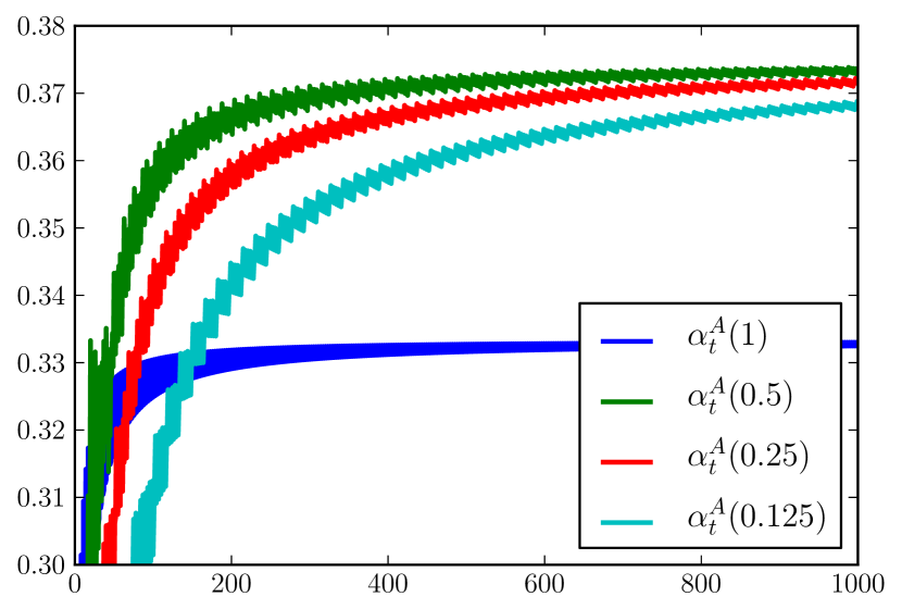
Figure 2: Sanity check: shrinkage leads to margin maximization.

Another question is how accurately the bounds presented here depict the methods provided. As a brief sanity check, the methods may be run on a problem instance where AdaBoost demonstrably does not achieve maximum margins. The particular instance tested here is a binary matrix $A\in\{-1,+1\}^{8\times 8}$ due to Rudin et al. (2004, Theorem 7); recall that AdaBoost, in the present notation (with $A$ binary), corresponds to $\ell=\exp$ and step size $\alpha_{t}^{\textup{A}}(1)=\alpha_{t}^{\textup{O}}(1)$ (no shrinkage). Two plots are provided.

1. Figure 2 is a sanity check, showing that $\ell=\exp$ and $\alpha_{t}^{\textup{A}}(1)=\alpha_{t}^{\textup{O}}(1)$ may not achieve maximum margins, but shrinkage overcomes this.

2. Figure 3 demonstrates that the Wolfe search (with $\ell=\exp$) is indeed effective, but demanding higher accuracy comes at a price.

These plots will be discussed further in Section 5. Additional tests with this matrix demonstrated that the method of Shalev-Shwartz & Singer (2008) indeed performs a tiny bit worse than the Wolfe search, but of course one example is not terribly indicative. Perhaps most importantly, a test with the logistic loss showed that the bound is loose: the logistic loss performs well, and does not suffer a startup cost as indicated by the bounds.

4 The General Case

The last technical contribution of this manuscript is to briefly consider the general case (which is potentially nonseparable). Similarly to the separable case, this section will establish convergence rates for empirical risk, margin guarantees, and briefly discuss the connection to existing margin maximizing methods. But first, it is necessary to discuss the structure of the general case, and in particular to develop what margins mean without separability.

This section hinges upon the following decomposition of a boosting instance. This decomposition partitions a boosting instance, specifically its examples $\{(x_{i},y_{i})\}_{i=1}^{m}$, into a hard subset $H(A)$, and an easy subset $H(A)^{c}$. The easy subset alone is separable, and thus margins will be measured there. Although the analysis will rely heavily on properties of this decomposition due to Telgarsky (2012), the decomposition itself has appeared, with various guarantees, in numerous places (Goldreich & Levin, 1989; Impagliazzo, 1995; Mukherjee et al., 2011). The notation $H(A)$ reflects the fact that this structure has no relation to the choice of $\ell\in\mathbb{L}$.

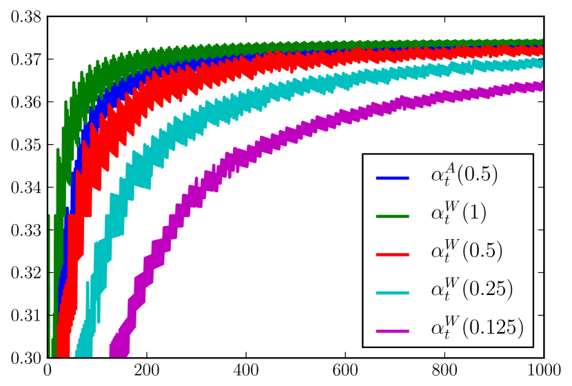
Figure 3: Sanity check: the Wolfe search effectively maximizes margins.

Definition 4.0.

(Cf. Telgarsky (2012, Definition 5.1, 5.7).) Given a boosting problem encoded in a matrix $A\in\mathbb{R}^{m\times n}$, a set of examples (rows) $H(A)\subseteq[m]$ is a hard core for $A$ (and the corresponding boosting problem) if it satisfies the following properties.

• There exists a weighting $\hat{\lambda}\in\mathbb{R}^{n}$ with $\textbf{e}_{i}^{\top}A\hat{\lambda}<0$ for $i\in H(A)^{c}$ and $\textbf{e}_{i}^{\top}A\hat{\lambda}=0$ for $i\in H(A)$.

• Every weighting $\lambda\in\mathbb{R}^{n}$ with $\textbf{e}_{i}^{\top}A\lambda<0$ for some $i\in H(A)$ also has $\textbf{e}_{k}^{\top}A\lambda>0$ for some $k\in H(A)$.

Additionally, define a row-wise partition of $A$ into matrices $A_{0},A_{+}$, where $A_{+}$ has the examples in $H(A)$, and $A_{0}$ has the examples in $H(A)^{c}$.

The second property provides that $H(A)$ is difficult: positive margins on some examples force negative margins on others. On the other hand, the complement $H(A)^{c}$ is easy, and moreover can be solved without affecting $H(A)$.

Proposition 4.0.

(Cf. Telgarsky (2012, Proposition 5.8, Theorem 5.9).) For any $A\in\mathbb{R}^{m\times n}$, a hard core $H(A)$ always exists, and is unique.

With the decomposition in place, the aforementioned guarantees may be stated. The first, as in the separable case, is convergence of empirical risk. There is hardly anything to do here; the groundwork from Section 3 can be plugged directly into existing techniques to generate this theorem (Telgarsky, 2012, Section 6).

Theorem 4.1.

Let general boosting matrix $A$ be given (i.e., potentially $\gamma=0$), along with shrinkage parameter $\nu\in(0,1]$, any $\ell\in\mathbb{L}$, and target suboptimality $\epsilon>0$. Suppose step sizes $\{\alpha_{t}\}_{t\geq 0}$ are consistent with $\alpha_{t}^{\textup{Q}}(\nu)$, $\alpha_{t}^{\textup{W}}(\nu)$, $\alpha_{t}^{\textup{O}}(\nu)$, or $\alpha_{t}^{\textup{A}}(\nu)$ with $\ell=\exp$ and $A$ binary. Then $\mathcal{O}(\frac{1}{\epsilon})$ iterations suffice to reach suboptimality $\epsilon>0$.

If the instance is either separable (i.e., $\gamma>0$ as in Section 3) or attains its minimizer (i.e., $|H(A)|=m$ (Telgarsky, 2012, Theorem 5.5)), then the rate improves to $\mathcal{O}(\ln(\frac{1}{\epsilon}))$.

Lastly come the margin guarantees. As stated above, $H(A)^{c}$, considered alone, is separable; note furthermore that the definition of hard core provides the existence of a weighting $\hat{\lambda}$. which has positive margins over $H(A)^{c}$, but abstains entirely over $H(A)$. Consequently, an approximate minimizer to $\mathcal{L}(A\cdot)$ can always add in a scaling of $\hat{\lambda}$ and improve its empirical risk while simultaneously improving margins over $H(A)^{c}$. Consequently, it is natural to expect the methods here to achieve positive margins over $H(A)^{c}$. Note that the following result only shows that some positive margins are attained, and neither assert some sense under which they are maximal, nor does it provide rates.

Theorem 4.2.

Let general boosting matrix $A$ be given with $1\leq|H(A)|\leq m-1$ (i.e., the problem is neither separable, nor is the minimizer attainable). Let shrinkage parameter $\nu\in(0,1]$ and any $\ell\in\mathbb{L}_{\infty}$ be given. Suppose step sizes $\{\alpha_{t}\}_{t\geq 0}$ are consistent with $\alpha_{t}^{\textup{Q}}(\nu)$, $\alpha_{t}^{\textup{W}}(\nu)$, $\alpha_{t}^{\textup{O}}(\nu)$ with $\ell=\exp$ and binary $A$, or $\alpha_{t}^{\textup{A}}(\nu)$ with $\ell=\exp$ and binary $A$., Then there exists $\hat{\gamma}>0$ so that every example off the hard core (i.e., $i\in H(A)^{c}$) has margin at least $\hat{\gamma}$ for all large $t$.

To close, consider once again the comparison to explicit margin maximizing boosting methods as presented by Shalev-Shwartz & Singer (2008). There is no point in discussing the specific method discussed in Section 3.3, whose optimal objective value is exactly $\gamma$, which in this case is zero, and the method may happily quit without iterating. Indeed, a primary contribution of Shalev-Shwartz & Singer (2008) is not only to address this issue, but show how the same general boosting scheme can be instantiated for the aforementioned method, as well as methods with tolerance to nonseparability.

Indeed, consider the “soft-margin” boosting method (Shalev-Shwartz & Singer, 2008), originally due to Warmuth et al. (2006), which, roughly speaking, has a parameter controlling how many examples to give up on. This is in contrast to the methods here, which not only have a fixed data-dependant structure they try less hard on (the hard core $H(A)$), but moreover the particular margins achieved over the hard core are determined by the loss function $\ell\in\mathbb{L}$. It is of course worth mentioning that the margin analysis in the nonseparable case here is by comparison very incomplete, providing no rates and not even identifying exactly what positive margins are attained.

5 Discussion

This manuscript immediately raises a number of questions. Perhaps foremost is the general question of the impact of margins on the efficacy of boosting. Although margins certainly provide an intuitive theory, it is still unclear how much they directly correlate with good algorithms (Reyzin & Schapire, 2006).

Next, the bounds for the logistic loss are not tight. As there do not appear to be any more forgiving analyses of the logistic loss, the natural question is whether there are new techniques which provide a better characterization.

Lastly, Figure 2 shows a threshold effect: shrinkage $1$ does not lead to the right margin, but $1/2$ and smaller suffices to reach the maximum margin. (Indeed, experimentation reveals the threshold to be roughly 0.92.) It should be possible to clarify this behavior from the perspective of dynamical systems: smaller steps dodge bad attractors (Rudin et al., 2004, 2007).

Acknowledgements

The author thanks Daniel Hsu and the ICML reviewers for helpful comments and discussions. The author is also deeply indebted to Robert Schapire for numerous discussions, insight, and for suggesting study of the unconstrained step size (at the time, guarantees were only in place for the other choices!). This work was graciously supported by the NSF under grant IIS-0713540.

Appendix A Deferred Material from Section 2

Proof of Section 2.1.

There is nothing to show for $\exp$, so consider $\ell(x)=\ln(1+\exp(x))$, let $z\in\mathbb{R}$ be given, and let $x\leq z$ be arbitrary.

Concavity grants $\ln(1+\exp(x))\leq\exp(x)$. The lower bound can be checked in two stages. First, if $x\leq\min\{-1,z\}$, a Taylor expansion gives

$$\ln(1+e^{x}) \geq e^{x}-\sup_{\xi\in\mathbb{R}}\frac{1}{2(1+\xi)^{2}}e^{2x}$$

$$\geq e^{x}\left(1-\frac{\min\{e^{z},e^{-1}\}}{2}\right).$$

On the other hand, if $-1\leq x\leq z$, then $e^{x}\leq e^{z}\ln(1+e^{-1})/\ln(1+e^{-1})\leq e^{z}\ln(1+e^{x})/\ln(1+e^{-1})$.

Next, $\ell^{\prime}(x)=e^{x}/(1+e^{x})$, so $\ell^{\prime}(x)\leq e^{x}\leq\ell^{\prime}(x)(1+e^{z})$. Similarly, $\ell^{\prime\prime}(x)=e^{x}/(1+e^{x})^{2}$, so $\ell^{\prime\prime}(x)\leq e^{x}\leq\ell^{\prime\prime}(x)(1+e^{z})^{2}$. ∎

The following appendix (and its proof) derive $\alpha_{t}^{\textup{Q}}(\nu)$, establishes $\alpha_{t}^{\textup{Q}}(\nu)\leq\alpha_{t}^{\textup{O}}(\nu)$, and gives the basic improvement due to one step satisfying $\alpha\in[\alpha_{t}^{\textup{Q}}(\nu),\alpha_{t}^{\textup{O}}(\nu)]$.

Lemma A.0.

Let boosting matrix $A$, shrinkage parameter $\nu\in(0,1]$, and any $\ell\in\mathbb{L}$ be given. For any iteration $t$, it holds that $\alpha_{t+1}^{\textup{Q}}(\nu)\leq\alpha_{t+1}^{\textup{O}}(\nu)$. Furthermore, any step $\alpha\in[\alpha_{t+1}^{\textup{Q}}(\nu),\alpha_{t+1}^{\textup{O}}(\nu)]$ satisfies

$$\mathcal{L}(A(\lambda_{t}+\alpha v_{t+1}))\leq\mathcal{L}(A\lambda_{t})\exp\left(-\frac{\nu(2-\nu)\gamma_{t+1}^{2}}{2C_{t+1}^{6}}\right).$$

Proof.

This analysis follows a scheme laid out by Telgarsky (2012, Appendix D.3). Let $t$ denote any fixed iteration, and $I$ denote the (possibly unbounded) interval

$$I:=\left\{\alpha\geq 0:\mathcal{L}(A(\lambda_{t}+\alpha v_{t+1}))\leq\mathcal{L}(A\lambda_{t})\right\};$$

by continuity of $\mathcal{L}$ and choice of $v_{t+1}$, $I$ is nonempty, with nonempty interior. By second order Taylor expansion, every $\alpha\in I$ satisfies

$$\mathcal{L}(A(\lambda_{t}+\alpha v_{t+1}))$$

$$\leq\mathcal{L}(A\lambda_{t})+\alpha v_{t+1}^{\top}A^{\top}\nabla\mathcal{L}(A\lambda_{t})$$

$$\quad+\sup_{r\in I}\frac{\alpha^{2}}{2}v_{t+1}^{\top}A^{\top}\nabla^{2}\mathcal{L}(A(\lambda_{t}+rv_{t+1}))Av_{t+1}$$

$$\leq\mathcal{L}(A\lambda_{t})-\alpha\|A^{\top}\nabla\mathcal{L}(A\lambda_{t})\|_{\infty}$$

$$\quad+\frac{\alpha^{2}}{2}\sup_{r\in I}\frac{1}{m}\sum_{i=1}^{m}\ell^{\prime\prime}(\textbf{e}_{i}^{\top}A(\lambda_{t}+rv_{t+1}))A_{ij_{t+1}}^{2}$$

$$\leq\mathcal{L}(A\lambda_{t})-\alpha\|A^{\top}\nabla\mathcal{L}(A\lambda_{t})\|_{\infty}$$

$$\quad+\frac{C_{t+1}^{2}\alpha^{2}}{2}\sup_{r\in I}\frac{1}{m}\sum_{i=1}^{m}\ell(\textbf{e}_{i}^{\top}A(\lambda_{t}+rv_{t+1}))A_{ij_{t+1}}^{2}$$

$$=\mathcal{L}(A\lambda_{t})-\alpha\|A^{\top}\nabla\mathcal{L}(A\lambda_{t})\|_{\infty}+\frac{C_{t+1}^{2}\alpha^{2}}{2}\mathcal{L}(A\lambda_{t})$$

$$\leq\mathcal{L}(A\lambda_{t})-\alpha\|A^{\top}\nabla\mathcal{L}(A\lambda_{t})\|_{\infty}+\frac{C_{t+1}^{4}\alpha^{2}}{2}\|\nabla\mathcal{L}(A\lambda_{t})\|_{1},$$

which made use of $\ell^{\prime\prime}\leq C_{t+1}\exp\leq C_{t+1}^{2}\ell$ along $I$, $\ell\leq C_{t+1}\exp\leq C_{t+1}^{2}\ell^{\prime}$ along $I$, $|A_{ij}|\leq 1$ (since elements of $\mathcal{H}$ are bounded in this way), and the definition of $I$ (specifically $r=0$ is the worst choice for $r\in I$). This final expression is a quadratic, whose minimizer must lie within $I$ (since its second derivative exceeds that of $\mathcal{L}$ along this interval). Differentiating and setting to zero, the minimizer is

$$I\ni\frac{\|A^{\top}\nabla\mathcal{L}(A\lambda_{t})\|_{\infty}}{C_{t+1}^{4}\|\nabla\mathcal{L}(A\lambda_{t})\|_{1}}=\frac{\gamma_{t+1}}{C_{t+1}^{4}}=\alpha_{t+1}^{\textup{Q}}(1).$$

This provides a derivation of the step $\alpha_{t+1}^{\textup{Q}}(\nu)$, and also shows $\alpha_{t+1}^{\textup{Q}}(1)\leq\alpha_{t+1}^{\textup{O}}(1)$. Plugging $\alpha_{t+1}^{\textup{Q}}(\nu)$ in for $\alpha$ in the above quadratic upper bound,

$$\mathcal{L}(A(\lambda_{t}+\alpha v_{t+1})) \leq\mathcal{L}(A\lambda_{t})-\frac{\nu(2-\nu)\gamma_{t+1}^{2}\|\nabla\mathcal{L}(A\lambda_{t})\|_{1}}{2C_{t+1}^{4}}$$

$$\leq\mathcal{L}(A\lambda_{t})\left(1-\frac{\nu(2-\nu)\gamma_{t+1}^{2}}{2C_{t+1}^{6}}\right)$$

$$\leq\mathcal{L}(A\lambda_{t})\exp\left(-\frac{\nu(2-\nu)\gamma_{t+1}^{2}}{2C_{t+1}^{6}}\right).$$

∎

Proof of Section 2.2.

This is the first part of Appendix A. ∎

Appendix B Deferred Material from Section 3

B.1 Deferred Material from Section 3.1

Proof of Section 3.1.

By Appendix A, for any $t$,

$$\mathcal{L}(A(\lambda_{t}+\alpha v_{t+1})) \leq\mathcal{L}(A\lambda_{t})\exp\left(-\frac{\nu(2-\nu)\gamma_{t+1}^{2}}{2C_{t+1}^{6}}\right).$$

Now let $t_{0}\leq t$ be given as in the desired statement, apply this bound $t-t_{0}$ times, and use the fact that $C_{t+1}\leq C_{t}$. ∎

Proof of Section 3.1.

Let $t$ denote any fixed iteration. Substituting $c_{1}=1-\nu/2$, $c_{2}=1-\nu/4$, and $\eta=C_{t+1}^{2}$ in a nearly identical guarantee for the Wolfe line search (Telgarsky, 2012, Proposition D.6) (where $\eta$ is simply the biggest ratio between $\ell$ and $\ell^{\prime\prime}$ in the current sublevel set) provides

$$\mathcal{L}(A(\lambda_{t}+\alpha v_{t+1}))$$

$$\leq\mathcal{L}(A\lambda_{t})-\frac{(1-\nu/2)(\nu/4)\|A^{\top}\nabla\mathcal{L}(A\lambda_{t})\|_{\infty}^{2}}{2C_{t+1}^{2}\mathcal{L}(A\lambda_{t})}$$

$$\leq\mathcal{L}(A\lambda_{t})\left(1-\frac{\nu(2-\nu)\gamma_{t+1}^{2}}{8C_{t+1}^{6}}\right)$$

$$\leq\mathcal{L}(A\lambda_{t})\exp\left(-\frac{\nu(2-\nu)\gamma_{t+1}^{2}}{8C_{t+1}^{6}}\right).$$

Given $t_{0}\leq t$, applying this bound $t-t_{0}$ times and using $C_{t+1}\leq C_{t}$ gives the result. ∎

Next, instead of directly proving Section 3.1, a more general section is given first, which will be useful later.

Lemma B.0.

Consider the setting of Theorem 3.1, except now each step size $\alpha_{i}$ satisfies

$$\alpha_{i}^{\textup{A}}(\nu)-\tau\leq\alpha_{i}\leq\alpha_{i}^{\textup{A}}(\nu)+\tau$$

for some $\tau>0$. Then, given $t\geq t_{0}$,

$$\mathcal{L}(A\lambda_{t+1})$$

$$\leq\mathcal{L}(A\lambda_{t_{0}})$$

$$\quad\cdot\prod_{i=t_{0}+1}^{t+1}\frac{e^{\tau}C_{i}^{4}}{2}(1-\gamma_{i}^{2})^{\nu/2}((1+\gamma_{i})^{1-\nu}+(1-\gamma_{i})^{1-\nu})$$

$$\leq\mathcal{L}(A\lambda_{t_{0}})\prod_{i=t_{0}+1}^{t+1}\frac{e^{\tau}C_{i}^{4}}{2}(1-\gamma_{i}^{2})^{\nu/2}.$$

Proof.

Fix an iteration $t$, and set $w_{i}=\ell^{\prime}(\textbf{e}_{i}^{\top}A\lambda_{t})$ and $W=\sum_{i}w_{i}\leq mC_{t+1}^{2}\mathcal{L}(A\lambda_{t})$. By convexity of $\exp(\cdot)$,

$$\mathcal{L}(A\lambda_{t+1})$$

$$\leq\frac{C_{t+1}}{m}\sum_{i=1}^{m}\exp(\textbf{e}_{i}^{\top}A\lambda_{t+1})$$

$$\leq\frac{C_{t+1}^{2}}{m}\left(\frac{W}{W}\right)\sum_{i=1}^{m}w_{i}\exp\Bigg{(}\frac{1+\textbf{e}_{i}^{\top}Av_{t+1}}{2}\alpha_{t+1}$$

$$\qquad\qquad+\frac{1-\textbf{e}_{i}^{\top}Av_{t+1}}{2}(-\alpha_{t+1})\Bigg{)}$$

$$\leq\frac{C_{t+1}^{2}}{m}W\left(\frac{1-\gamma_{t+1}}{2}\exp(\alpha_{t+1})+\frac{1+\gamma_{t+1}}{2}\exp(-\alpha_{t+1})\right)$$

$$\leq\frac{e^{\tau}C_{t+1}^{4}}{2}\mathcal{L}(A\lambda_{t})(1-\gamma_{t+1}^{2})^{\nu/2}$$

$$\quad\cdot\left((1-\gamma_{t+1})^{1-\nu}+(1+\gamma_{t+1})^{1-\nu}\right).$$

To simplify this expression, note that $(\cdot)^{1-\nu}$ is a concave function, and thus

$$\frac{(1-\gamma_{t+1})^{1-\nu}}{2}+\frac{(1+\gamma_{t+1})^{1-\nu}}{2}$$

$$\leq\left(\frac{1-\gamma_{t+1}}{2}+\frac{1+\gamma_{t+1}}{2}\right)^{1-\nu}$$

$$=1.$$

To finish, given $t\geq t_{0}$, the result follows by $t-t_{0}$ applications of these bounds. ∎

Proof of Section 3.1.

This follows by taking the second bound in Section B.1 with the choice $\tau=0$. ∎

Proof of Theorem 3.1.

The result follows from Section 3.1, Section 3.1, and Section 3.1 with the choice $t_{0}=0$ and using $C_{t+1}\leq C_{t}$. ∎

B.2 Deferred Material from Section 3.2

Proof of Section 3.2.

To start, note that

$$\|\lambda_{t+1}\|_{1} =\left\|\nu\sum_{i=1}^{t+1}v_{i}\gamma_{i}C_{i}^{-4}\right\|_{1}\leq\nu C_{1}^{-4}\sum_{i=1}^{t+1}\gamma_{i}\leq\nu\sum_{i=1}^{t+1}\gamma_{i}.$$

By the form of $\mathcal{L}$ and the optimization guarantee in Section 3.1,

$$\max_{k\in[m]}\exp(\textbf{e}_{k}^{\top}A\lambda_{t+1})$$

$$\leq\sum_{i=1}^{m}\exp(\textbf{e}_{i}^{\top}A\lambda_{t+1})$$

$$\leq mC_{t+1}\mathcal{L}(A\lambda_{t+1})$$

$$\leq mC_{t_{0}+1}\mathcal{L}(A\lambda_{t_{0}})\exp\left(-\frac{\nu(2-\nu)}{2C_{t_{0}+1}^{6}}\sum_{i=t_{0}+1}^{t+1}\gamma_{i}^{2}\right)$$

$$=mC_{t_{0}+1}\mathcal{L}(A\lambda_{t_{0}})\exp\left(\frac{\nu(2-\nu)}{2C_{t_{0}+1}^{6}}\sum_{i=1}^{t_{0}}\gamma_{i}^{2}\right)$$

$$\quad\cdot\exp\left(-\frac{\nu(2-\nu)}{2C_{t_{0}+1}^{6}}\sum_{i=1}^{t+1}\gamma_{i}^{2}\right)$$

$$\leq c_{0}\exp\left(-\frac{(2-\nu)}{2C_{t_{0}+1}^{6}}\sum_{i=1}^{t}\nu\gamma_{i}^{2}\right),$$

where $c_{0}$ is as in the statement. Since $\ln(\cdot)$ is increasing, it follows that

$$\max_{k\in[m]}\textbf{e}_{k}^{\top}A\lambda_{t+1}\leq-\frac{(2-\nu)}{2C_{t_{0}+1}^{6}}\sum_{i=1}^{t}\nu\gamma_{i}^{2}+\ln(c_{0}).$$

Using the above bound on $\|\lambda_{t}\|_{1}$, since $t\gamma\leq\sum_{i=1}^{t+1}\gamma_{t}$, and $-\textbf{e}_{k}^{\top}A\lambda_{t+1}$ is nonnegative by the lower bound on $t$,

$$\min_{k\in[m]}\frac{-\textbf{e}_{k}^{\top}A\lambda_{t+1}}{\|\lambda_{t+1}\|_{1}} \geq\min_{k\in[m]}\frac{-\textbf{e}_{k}^{\top}A\lambda_{t+1}}{\nu\sum_{i=1}^{t+1}\gamma_{i}}$$

$$\geq\gamma\left(\frac{2-\nu}{2C_{t_{0}+1}^{6}}\right)-\frac{\ln(c_{0})}{\nu\sum_{i=1}^{t+1}\gamma_{i}}$$

$$\geq\gamma\left(\frac{2-\nu}{2C_{t_{0}+1}^{6}}\right)-\frac{\ln(c_{0})}{(t+1)\nu\gamma}.\qed$$

Proof of Section 3.2.

Any step size $\alpha_{t+1}$ satisfying the Wolfe conditions will have lower bound

$$\alpha_{t+1} \geq\frac{(1-(1-\nu/4))\|A^{\top}\mathcal{L}(A\lambda_{t})\|_{\infty}}{C_{t}^{2}\mathcal{L}(A\lambda_{t})}$$

$$\geq\frac{(1-(1-\nu/4))\|A^{\top}\mathcal{L}(A\lambda_{t})\|_{\infty}}{C_{t}^{4}\|\nabla\mathcal{L}(A\lambda_{t})\|_{1}}$$

$$=\frac{\nu\gamma_{t+1}}{4C_{t+1}^{4}}\geq\frac{\nu\gamma}{4C_{1}^{4}};$$

indeed this expression appears in proofs demonstrating the improvement due to a single step of the Wolfe search, see for instance Telgarsky (2012, Proof of Proposition D.6, second to last line).

Additionally, note

$$\|\lambda_{t+1}\|_{1}=\left\|\sum_{i=1}^{t+1}\alpha_{i}v_{i}\right\|_{1}\leq\sum_{i=1}^{t+1}\alpha_{i}.$$

Direct from the first Wolfe condition (eq. 2.1),

$$\mathcal{L}(A\lambda_{t+1})$$

$$=\mathcal{L}(A(\lambda_{t}+\alpha_{t+1}v_{t+1}))$$

$$\leq\mathcal{L}(A\lambda_{t})-\alpha_{t+1}(1-\nu/2)\|A^{\top}\nabla\mathcal{L}(A\lambda_{t})\|_{\infty}$$

$$\leq\mathcal{L}(A\lambda_{t})\left(1-\frac{\alpha_{t+1}(1-\nu/2)\|A^{\top}\nabla\mathcal{L}(A\lambda_{t})\|_{\infty}}{\mathcal{L}(A\lambda_{t})}\right)$$

$$\leq\mathcal{L}(A\lambda_{t})\left(1-\frac{\alpha_{t+1}(2-\nu)\gamma_{t+1}}{2C_{t+1}^{2}}\right).$$

Now let $t\geq t_{0}$ be given as in the statement. Applying the above inequality $t-t_{0}$ times,

$$\max_{k\in[m]}\exp(\textbf{e}_{k}^{\top}A\lambda_{t+1})$$

$$\leq mC_{t+1}\mathcal{L}(A\lambda_{t+1})$$

$$\leq mC_{t_{0}+1}\mathcal{L}(A\lambda_{t_{0}})\exp\left(-\frac{(2-\nu)\gamma}{2C_{t_{0}+1}^{2}}\sum_{i=t_{0}+1}^{t+1}\alpha_{i}\right)$$

$$\leq mC_{t_{0}+1}\mathcal{L}(A\lambda_{t_{0}})\exp\left(\frac{(2-\nu)\gamma}{2C_{t_{0}+1}^{2}}\sum_{i=1}^{t_{0}}\alpha_{i}\right)$$

$$\quad\cdot\exp\left(-\frac{(2-\nu)\gamma}{2C_{t_{0}+1}^{2}}\sum_{i=1}^{t+1}\alpha_{i}\right)$$

$$\leq c_{0}\exp\left(-\frac{(2-\nu)\gamma}{2C_{t_{0}+1}^{2}}\sum_{i=1}^{t+1}\alpha_{i}\right),$$

where $c_{0}$ is as in the statement. Since $\ln(\cdot)$ is increasing, it follows that

$$\max_{k\in[m]}\textbf{e}_{k}^{\top}A\lambda_{t+1}\leq-\frac{(2-\nu)\gamma}{2C_{t_{0}+1}^{2}}\sum_{i=1}^{t+1}\alpha_{i}+\ln(c_{0}).$$

Using the above lower bound on $\alpha_{i}$ in terms of $\gamma_{i}$, and since all margins are nonnegative by the lower bound on $t$,

$$\min_{k\in[m]}\frac{-\textbf{e}_{k}^{\top}A\lambda_{t+1}}{\|\lambda_{t+1}\|_{1}} \geq\min_{k\in[m]}\frac{-\textbf{e}_{k}^{\top}A\lambda_{t+1}}{\sum_{i=1}^{t+1}\alpha_{i}}$$

$$\geq\gamma\left(\frac{2-\nu}{2C_{t_{0}+1}^{2}}\right)-\frac{\ln(c_{0})}{\sum_{i=1}^{t+1}\alpha_{i}}$$

$$\geq\gamma\left(\frac{2-\nu}{2C_{t_{0}+1}^{2}}\right)-\frac{4C_{1}^{4}\ln(c_{0})}{(t+1)\nu\gamma}.\qed$$

The remainder of this subsection provides proofs for $\alpha_{t}^{\textup{A}}(\nu)$ and $\alpha_{t}^{\textup{O}}(\nu)$, but uses some later material, most specifically the quantity $\Upsilon_{\nu}$.

Lemma B.0.

Consider the setting of Theorem 3.1, except now each step size $\alpha_{i}$ satisfies

$$\alpha_{i}^{\textup{A}}(\nu)-\tau\leq\alpha_{i}\leq\alpha_{i}^{\textup{A}}(\nu)+\tau$$

for some $\tau>0$. Let $\theta\in[0,\gamma)$ be given. Then, given $t\geq t_{0}$,

$$\sum_{i=1}^{m}\mathds{1}\left[\frac{-\textbf{e}_{i}A\lambda_{t+1}}{\|\lambda_{t+1}\|_{1}}<\theta\right]$$

$$\leq mC_{t+1}\exp(\theta\|\lambda_{t_{0}}\|_{1})\mathcal{L}(A\lambda_{t_{0}})\prod_{i=t_{0}+1}^{t+1}\Bigg{(}e^{\theta\tau}\left(\frac{1+\gamma_{i}}{1-\gamma_{i}}\right)^{\theta\nu/2}$$

$$\quad\cdot\frac{e^{\tau}C_{i}^{4}}{2}(1-\gamma_{i}^{2})^{\nu/2}((1+\gamma_{i})^{1-\nu}+(1-\gamma_{i})^{1-\nu})\Bigg{)}.$$

$$\leq mC_{t+1}\exp(\theta\|\lambda_{t_{0}}\|_{1})\mathcal{L}(A\lambda_{t_{0}})\prod_{i=t_{0}+1}^{t+1}\Bigg{(}e^{\theta\tau}\left(\frac{1+\gamma_{i}}{1-\gamma_{i}}\right)^{\theta\nu/2}$$

$$\quad\cdot e^{\tau}C_{i}^{4}(1-\gamma_{i}^{2})^{\nu/2}\Bigg{)}.$$

Proof.

To start,

$$\sum_{i=1}^{m}\mathds{1}\left[\frac{-\textbf{e}_{i}A\lambda_{t+1}}{\|\lambda_{t+1}\|_{1}}<\theta\right]$$

$$=\sum_{i=1}^{m}\mathds{1}\left[\theta\|\lambda_{t+1}\|_{1}+\textbf{e}_{i}A\lambda_{t+1}>0\right]$$

$$\leq mC_{t+1}\exp(\theta\|\lambda_{t+1}\|_{1})\mathcal{L}(A\lambda_{t+1}).$$

Next, note

$$\|\lambda_{t+1}\|_{1} =\left\|\lambda_{t_{0}}+\sum_{i=t_{0}+1}^{t+1}\alpha_{i}v_{i}\right\|_{1}$$

$$\leq\|\lambda_{t_{0}}\|_{1}+\sum_{i=t_{0}+1}^{t+1}(\tau+\alpha_{i}^{\textup{A}}(\nu)).$$

Combining these facts with the convergence bound from Section B.1,

$$\sum_{i=1}^{m}\mathds{1}\left[\frac{-\textbf{e}_{i}A\lambda_{t+1}}{\|\lambda_{t+1}\|_{1}}<\theta\right]$$

$$\leq mC_{t+1}\exp(\theta\|\lambda_{t_{0}}\|_{1})\mathcal{L}(A\lambda_{t_{0}})\prod_{i=t_{0}+1}^{t+1}\Bigg{(}e^{\theta\tau}\left(\frac{1+\gamma_{i}}{1-\gamma_{i}}\right)^{\theta\nu/2}$$

$$\quad\cdot\frac{e^{\tau}C_{i}^{4}}{2}(1-\gamma_{i}^{2})^{\nu/2}((1+\gamma_{i})^{1-\nu}+(1-\gamma_{i})^{1-\nu})\Bigg{)}.$$

As in the proof of Section B.1, $(\cdot)^{1-\nu}$ is concave, so the $1/2$ may be pushed inside this last term to give the vaguely simpler bound

$$\sum_{i=1}^{m}\mathds{1}\left[\frac{-\textbf{e}_{i}A\lambda_{t+1}}{\|\lambda_{t+1}\|_{1}}<\theta\right]$$

$$\leq mC_{t+1}\exp(\theta\|\lambda_{t_{0}}\|_{1})\mathcal{L}(A\lambda_{t_{0}})\prod_{i=t_{0}+1}^{t+1}\Bigg{(}e^{\theta\tau}\left(\frac{1+\gamma_{i}}{1-\gamma_{i}}\right)^{\theta\nu/2}$$

$$\quad\cdot e^{\tau}C_{i}^{4}(1-\gamma_{i}^{2})^{\nu/2}\Bigg{)}.\qed$$

Proof of Section 3.2.

Set $\theta:=\gamma-\epsilon$, whereby $\theta\in[0,\gamma)$. Invoking Section B.2 and simplifying terms via $t_{0}=0$, $C_{i}=1$, and $\tau=0$, then for any $t$,

$$\sum_{i=1}^{m}\mathds{1}\left[\frac{-\textbf{e}_{i}A\lambda_{t+1}}{\|\lambda_{t+1}\|_{1}}<\theta\right]$$

$$\leq m\prod_{i=1}^{t+1}\Bigg{(}\left(\frac{1+\gamma_{i}}{1-\gamma_{i}}\right)^{\theta\nu/2}$$

$$\quad\cdot\frac{1}{2}(1-\gamma_{i}^{2})^{\nu/2}((1+\gamma_{i})^{1-\nu}+(1-\gamma_{i})^{1-\nu})$$

$$\leq m\prod_{i=1}^{t+1}\Bigg{(}\left(\frac{1+\gamma}{1-\gamma}\right)^{\theta\nu/2}$$

$$\quad\cdot\frac{1}{2}(1-\gamma^{2})^{\nu/2}((1+\gamma)^{1-\nu}+(1-\gamma)^{1-\nu})\Bigg{)},$$

where the replacement of $\gamma_{i}$ by $\gamma$ made use of the first part of Section B.2.1. Now, by the second part of Section B.2.1, this inner term is less than 1 iff $\theta<\Upsilon_{\nu}(\gamma)$. By Theorem B.2, since $\theta<\gamma$, there exists a $\nu$ sufficiently small that $\Upsilon_{\nu}(\gamma)>\theta$. Consequently, there exists a $T$ so that this product is less than $1/m$ whenever $t\geq T$, and the result follows. ∎

Proof of Section 3.2.

Set $\theta:=\gamma-\epsilon$, whereby $\theta\in[0,\gamma)$. Since $\ell\in L_{\infty}$, choose $t_{0}$ large enough so that

$$C_{t_{0}}^{8}<\left(\frac{1+\gamma}{1-\gamma}\right)^{\frac{(\gamma-\theta)\nu}{4}}.$$

By Section B.2.2, it follows that the optimal step size satisfies

$$\alpha_{t}^{\textup{A}}(\nu)-\tau\leq\alpha_{t}^{\textup{O}}(\nu)\leq\alpha_{t}^{\textup{A}}(\nu)+\tau$$

with $\tau=\frac{\nu}{2}\ln(C_{t}^{4})$. Combining this with the bound on $C_{t_{0}}$ above,

$$e^{2\tau}C_{t_{0}}^{4}=C_{t_{0}}^{8}<\left(\frac{1+\gamma}{1-\gamma}\right)^{\frac{(\gamma-\theta)\nu}{4}}.$$

Plugging this into the general margin bound in Section B.2 and additionally replacing $\gamma_{i}$ with $\gamma$ thanks to the first part of Section B.2.1, and finally setting $\theta^{\prime}:=\theta+(\gamma-\theta)/2=(\theta+\gamma)/2<\gamma$,

$$\sum_{i=1}^{m}\mathds{1}\left[\frac{-\textbf{e}_{i}A\lambda_{t+1}}{\|\lambda_{t+1}\|_{1}}<\theta\right]$$

$$\leq mC_{t+1}\exp(\theta\|\lambda_{t_{0}}\|_{1})\mathcal{L}(A\lambda_{t_{0}})$$

$$\quad\cdot\prod_{i=t_{0}+1}^{t+1}\Bigg{(}e^{\theta\tau}\left(\frac{1+\gamma_{i}}{1-\gamma_{i}}\right)^{\theta\nu/2}$$

$$\qquad\cdot\frac{e^{\tau}C_{i}^{4}}{2}(1-\gamma_{i}^{2})^{\nu/2}((1+\gamma_{i})^{1-\nu}+(1-\gamma_{i})^{1-\nu})\Bigg{)}$$

$$\leq mC_{t+1}\exp(\theta\|\lambda_{t_{0}}\|_{1})\mathcal{L}(A\lambda_{t_{0}})$$

$$\quad\cdot\prod_{i=t_{0}+1}^{t+1}\Bigg{(}e^{2\tau}C_{t_{0}+1}^{4}\left(\frac{1+\gamma}{1-\gamma}\right)^{\theta\nu/2}$$

$$\qquad\cdot\frac{1}{2}(1-\gamma^{2})^{\nu/2}((1+\gamma)^{1-\nu}+(1-\gamma)^{1-\nu})\Bigg{)}$$

$$\leq mC_{t+1}\exp(\theta\|\lambda_{t_{0}}\|_{1})\mathcal{L}(A\lambda_{t_{0}})$$

$$\quad\cdot\prod_{i=t_{0}+1}^{t+1}\Bigg{(}\left(\frac{1+\gamma}{1-\gamma}\right)^{\theta^{\prime}\nu/2}$$

$$\qquad\cdot\frac{1}{2}(1-\gamma^{2})^{\nu/2}((1+\gamma)^{1-\nu}+(1-\gamma)^{1-\nu})\Bigg{)}.$$

By the second part of Section B.2.1, the term within the product is less than one, and thus for all large $t$, this entire bound is less than $1$, which gives the result. ∎

Proof of Section 3.2.

To start, note that, for any $t\geq 0$,

$$(1-\gamma_{t})^{1-\theta}(1+\gamma_{t})^{1+\theta} =(1-\gamma_{t}^{2})^{1-\theta}(1+\gamma_{t})^{2\theta}$$

$$\leq\exp\left(-\gamma_{t}^{2}(1-\theta)+\gamma_{t}(2\theta)\right)$$

$$=\exp\left(-\gamma_{t}^{2}+\theta\gamma_{t}(2+\gamma_{t})\right).$$ (B.1)

Next, since

$$\theta\leq\frac{\gamma}{1+\gamma}=\frac{1}{1+1/\gamma}\leq\frac{1}{1+1/\gamma_{t}}=\frac{\gamma_{t}}{1+\gamma_{t}},$$

then $\theta\leq\gamma/(1+\gamma)$ implies

$$\frac{d}{d\gamma_{t}}\left(-\gamma_{t}^{2}+\theta\gamma_{t}(2+\gamma_{t})\right) =-2\gamma_{t}+2\theta(1+\gamma_{t})$$

$$\leq-2\gamma_{t}+2\gamma_{t}$$

$$=0.$$

In particular, the expression $-\gamma_{t}^{2}+\theta\gamma_{t}(2+\gamma_{t})$ is decreasing in $\gamma$, and thus $\gamma_{t}\geq\gamma$ implies

$$-\gamma_{t}^{2}+\theta\gamma_{t}(2+\gamma_{t})\leq-\gamma^{2}+\theta\gamma(2+\gamma),$$

and consequently, combined with the bound in (B.1),

$$(1-\gamma_{t})^{1-\theta}(1+\gamma_{t})^{1+\theta}\leq\exp(-\gamma^{2}+\theta\gamma(2+\gamma)).$$

Plugging this into the simplified generic bound in Section B.2 with the specialization $\ell=\exp$, $\tau=0$, $C_{i}=1$, and $t_{0}=0$, it follows that

$$\sum_{i=1}^{m}\mathds{1}\left[\frac{-\textbf{e}_{i}A\lambda_{t+1}}{\|\lambda_{t+1}\|_{1}}<\theta\right]$$

$$\leq m\prod_{i=1}^{t+1}\Bigg{(}\left(\frac{1+\gamma_{i}}{1-\gamma_{i}}\right)^{\theta\nu/2}(1-\gamma_{i}^{2})^{\nu/2}\Bigg{)}$$

$$\leq m\exp\left(-\frac{\nu(t+1)}{2}(-\gamma^{2}+\theta\gamma(2+\gamma))\right).$$

The rest of the result follows by noting $\theta<\gamma/(2+\gamma)$ implies $-\gamma^{2}+\theta\gamma(2+\gamma)<0$, whereby choices

$$t>\frac{2\ln(m)}{\nu(\gamma^{2}-\theta\gamma(2+\gamma))}$$

exist, and plugging this all in to the above bound grants that $\mathcal{M}(A\lambda_{t})\geq\theta$. ∎

Proof of Theorem 3.2.

For $\alpha_{t}^{\textup{A}}(\nu)$ and $\alpha_{t}^{\textup{O}}(\nu)$, Section 3.2 and Section 3.2 already state the results in the desired asymptotic form.

For the other two, since $\ell\in\mathbb{L}_{\infty}$, $t_{0}$ can be chosen sufficiently large so that $C_{t_{0}}$ is arbitrarily close to $1$, whereby the bounds in Section 3.2 and Section 3.2 become sufficiently tight by taking $\nu$ small and $t\nu$ large. ∎

B.2.1 The Quantity $\Upsilon_{\nu}$

Definition B.1.

Define

$$\Upsilon_{\nu}(\gamma):=$$

$$\frac{\frac{2}{\nu}\ln(2)-\frac{2}{\nu}\ln((1+\gamma)^{1-\nu}+(1-\gamma)^{1-\nu})-\ln(1-\gamma^{2})}{\ln(1+\gamma)-\ln(1-\gamma)};$$

in the case that $\nu=1$, this quantity has been extensively studied in the context of AdaBoost’s margins (Rätsch & Warmuth, 2005; Rudin et al., 2004; Schapire & Freund, 2012)

The basic properties of $\Upsilon_{\nu}$ are as follows.

Theorem B.2.

Suppose $\gamma\in(0,1)$.

1. $\gamma/2\leq\Upsilon_{\nu}(\gamma)\leq\gamma$.

2. $\lim_{\nu\downarrow 0}\Upsilon_{\nu}(\gamma)=\gamma$.

The bounds $\gamma/2\leq\Upsilon_{1}(\gamma)\leq\gamma$ were known in the case that $\nu=1$ (cf. Rätsch & Warmuth (2005) and Schapire & Freund (2012, Bibliographic Notes, Chapter 5)).

Proof.

(Item 1, subcase $\Upsilon_{\nu}(\gamma)\geq\gamma/2$.) To start, note that $(\cdot)^{1-\nu}$ is a concave function, whereby

$$-\frac{2}{\nu}\ln\left((1+\gamma)^{1-\nu}+(1-\gamma)^{1-\nu}\right)$$

$$=-\frac{2}{\nu}\ln\left(2\left(\frac{1}{2}(1+\gamma)^{1-\nu}+\frac{1}{2}(1-\gamma)^{1-\nu}\right)\right)$$

$$\geq-\frac{2}{\nu}\ln\left(2\left(1\right)^{1-\nu}\right)$$

$$=-\frac{2}{\nu}\ln\left(2\right).$$

It follows that

$$\Upsilon_{\nu}(\gamma)\geq\frac{-\ln(1-\gamma^{2})}{\ln(1+\gamma)-\ln(1-\gamma)}=\Upsilon_{1}(\gamma).$$

Next recall the series expansion

$$\ln(1+z)=\sum_{n=1}^{\infty}\frac{(-1)^{n+1}}{n}z^{n}$$

(when $|z|<1$). Plugging this in to the simplified form of $\Upsilon_{1}(\gamma)$ and paying attention to cancellations in the numerator and denominator (odd and even terms, respectively),

$$\Upsilon_{1}(\gamma) =\frac{-\sum_{n=1}^{\infty}\frac{(-1)^{n+1}}{n}(\gamma)^{n}-\sum_{n=1}^{\infty}\frac{(-1)^{n+1}}{n}(-\gamma)^{n}}{\sum_{n=1}^{\infty}\frac{(-1)^{n+1}}{n}(\gamma)^{n}-\sum_{n=1}^{\infty}\frac{(-1)^{n+1}}{n}(-\gamma)^{n}}$$

$$=\frac{-2\sum_{n=1}^{\infty}\frac{(-1)^{2n+1}}{2n}(\gamma)^{2n}}{2\sum_{n=1}^{\infty}\frac{(-1)^{2n-1+1}}{2n-1}(\gamma)^{2n-1}}$$

$$=\frac{\gamma\sum_{n=1}^{\infty}\frac{1}{2n}(\gamma)^{2n}}{\sum_{n=1}^{\infty}\frac{1}{2n-1}(\gamma)^{2n}}.$$

To finish, note that $n\geq 1$ implies $1/(4n-2)\leq 1/(2n)\leq 1/(2n-1)$, and thus

$$\frac{\gamma}{2} =\frac{\gamma\sum_{n=1}^{\infty}\frac{1}{2(2n-1)}(\gamma)^{2n}}{\sum_{n=1}^{\infty}\frac{1}{2n-1}(\gamma)^{2n}}$$

$$\leq\frac{\gamma\sum_{n=1}^{\infty}\frac{1}{2n}(\gamma)^{2n}}{\sum_{n=1}^{\infty}\frac{1}{2n-1}(\gamma)^{2n}}$$

$$\leq\frac{\gamma\sum_{n=1}^{\infty}\frac{1}{2n-1}(\gamma)^{2n}}{\sum_{n=1}^{\infty}\frac{1}{2n-1}(\gamma)^{2n}}$$

$$=\gamma.$$

That is to say, $\gamma/2\leq\Upsilon_{1}(\gamma)\leq\gamma$, which combined with the above also gives $\Upsilon_{\nu}(\gamma)\geq\Upsilon_{1}(\gamma)\geq\gamma/2$.

(Item 1, subcase $\Upsilon_{\nu}(\gamma)\leq\gamma$.) By the power mean inequality (Steele, 2004, Equation 8.12),

$$\left(\frac{1+\gamma}{2}(1+\gamma)^{-\nu}+\frac{1-\gamma}{2}(1-\gamma)^{-\nu}\right)^{-1/\nu}$$

$$\leq(1+\gamma)^{\frac{1+\gamma}{2}}(1-\gamma)^{\frac{1-\gamma}{2}}.$$

It follows that

$$-\frac{2}{\nu}\ln\left(\frac{1+\gamma}{2}(1+\gamma)^{-\nu}+\frac{1-\gamma}{2}(1-\gamma)^{-\nu}\right)$$

$$\leq(1+\gamma)\ln(1+\gamma)+(1-\gamma)\ln(1-\gamma).$$

As such,

$$\Upsilon_{\nu}(\gamma)$$

$$\leq\frac{(1+\gamma)\ln(1+\gamma)+(1-\gamma)\ln(1-\gamma)}{\ln(1+\gamma)-\ln(1-\gamma)}$$

$$\quad+\frac{-\ln(1+\gamma)-\ln(1-\gamma)}{\ln(1+\gamma)-\ln(1-\gamma)}$$

$$=\frac{\gamma\ln(1+\gamma)-\gamma\ln(1-\gamma)}{\ln(1+\gamma)-\ln(1-\gamma)}$$

$$=\gamma.$$

(Item 2.) Consider the (halved, negated) first term

$$\frac{\ln((1+\gamma)^{1-\nu}+(1-\gamma)^{1-\nu})-\ln(2)}{\nu}$$

$$=\frac{\ln(0.5(1+\gamma)^{1-\nu}+0.5(1-\gamma)^{1-\nu})}{\nu}.$$

By l’Hôpital’s rule,

$$\lim_{\nu\to 0}\frac{\ln(0.5(1+\gamma)^{1-\nu}+0.5(1-\gamma)^{1-\nu})}{\nu}$$

$$=\lim_{\nu\to 0}\frac{-(1+\gamma)^{1-\nu}\ln(1+\gamma)-(1-\gamma)^{1-\nu}\ln(1-\gamma)}{(1+\gamma)^{1-\nu}+(1-\gamma)^{1-\nu}}$$

$$=-\frac{1}{2}\left((1+\gamma)\ln(1+\gamma)+(1-\gamma)\ln(1-\gamma)\right).$$

Consequently (recalling that this term was both halved and negated)

$$\lim_{\nu\to 0}\Upsilon_{\nu}(\gamma) =\frac{(1+\gamma)\ln(1+\gamma)+(1-\gamma)\ln(1-\gamma)}{\ln(1+\gamma)-\ln(1-\gamma)}$$

$$\quad+\frac{-\ln(1+\gamma)-\ln(1-\gamma)}{\ln(1+\gamma)-\ln(1-\gamma)}$$

$$=\gamma.\qed$$

The usefulness of $\Upsilon_{\nu}$ is captured in the following section.

Lemma B.2.

Let $\nu\in(0,1]$ and $\theta\in[0,1]$ be given. The map

$$\gamma \mapsto\left(\frac{1+\gamma}{1-\gamma}\right)^{\theta\nu/2}(1-\gamma^{2})^{\nu/2}$$

$$\quad\cdot((1+\gamma)^{1-\nu}+(1-\gamma)^{1-\nu})$$

is nonincreasing over $[\theta,1]$. Additionally, now taking $\gamma$ to be fixed, $\theta<\Upsilon_{\nu}(\gamma)$ iff

$$\frac{1}{2}\left(\frac{1+\gamma}{1-\gamma}\right)^{\theta\nu/2}(1-\gamma^{2})^{\nu/2}$$

$$\quad\cdot((1+\gamma)^{1-\nu}+(1-\gamma)^{1-\nu})$$

$$<1.$$

Proof.

Let $f(\gamma)$ be the prescribed map. To establish $f$ is nonincreasing, it will be shown that each element of the product $f(\gamma)=g(\gamma)h(\gamma)$ is nonincreasing, where

$$g(\gamma) :=\left(\frac{1+\gamma}{1-\gamma}\right)^{\theta\nu/2}(1-\gamma^{2})^{\nu/2}$$

$$h(\gamma) :=(1+\gamma)^{1-\nu}+(1-\gamma)^{1-\nu}.$$

First, set $\nu^{\prime}:=\nu/2$, and note

$$g^{\prime}(\gamma) =\frac{d}{d\gamma}(1+\gamma)^{\nu^{\prime}(1+\theta)}(1-\gamma)^{\nu^{\prime}(1-\theta)}$$

$$=\nu^{\prime}(1+\theta)(1+\gamma)^{\nu^{\prime}(1+\theta)-1}(1-\gamma)^{\nu^{\prime}(1-\theta)}$$

$$\quad-\nu^{\prime}(1-\theta)(1-\gamma)^{\nu^{\prime}(1-\theta)-1}(1+\gamma)^{\nu^{\prime}(1+\theta)}$$

$$=\nu^{\prime}(1+\gamma)^{\nu^{\prime}(1+\theta)-1}(1-\gamma)^{\nu^{\prime}(1-\theta)-1}$$

$$\quad\cdot\left((1+\theta)(1-\gamma)-(1-\theta)(1+\gamma)\right)$$

$$=2\nu^{\prime}(1+\gamma)^{\nu^{\prime}(1+\theta)-1}(1-\gamma)^{\nu^{\prime}(1-\theta)-1}\left(\theta-\gamma\right),$$

where this last term is nonpositive since $\theta\leq\gamma$. Consequently, $g(\gamma)$ is nonincreasing.

For $h(\gamma)$, note similarly that

$$h^{\prime}(\gamma) =(1-\nu)\left((1+\gamma)^{-\nu}-(1-\gamma)^{-\nu}\right)$$

$$=\frac{1-\nu}{(1+\gamma)^{\nu}(1-\gamma)^{\nu}}\left((1-\gamma)^{\nu}-(1+\gamma)^{\nu}\right)$$

$$\leq 0.$$

Together $f(\gamma)=g(\gamma)h(\gamma)$ is nonincreasing in $\gamma$.

For the second statement, note that

$$1 >\frac{1}{2}\left(\frac{1+\gamma}{1-\gamma}\right)^{\theta\nu/2}(1-\gamma^{2})^{\nu/2}$$

$$\quad\cdot((1+\gamma)^{1-\nu}+(1-\gamma)^{1-\nu})$$

is equivalent to

$$0 >-\ln(2)+\frac{\nu}{2}\theta\ln\left(\frac{1+\gamma}{1-\gamma}\right)+\frac{\nu}{2}\ln(1-\gamma^{2})$$

$$\quad+\ln((1+\gamma)^{1-\nu}+(1-\gamma)^{1-\nu})$$

is equivalent to

$$\theta<$$

$$\frac{\ln(2)-\frac{\nu}{2}\ln(1-\gamma^{2})-\ln((1+\gamma)^{1-\nu}+(1-\gamma)^{1-\nu})}{\frac{\nu}{2}\ln\left(\frac{1+\gamma}{1-\gamma}\right)},$$

where the last expression can be written $\theta<\Upsilon_{\nu}(\gamma)$. ∎

B.2.2 Miscellaneous Technical Material

Lemma B.2.

Suppose $A\in\{-1,+1\}^{m\times n}$ is binary and $\ell\in\mathbb{L}$. Then

$$\frac{1}{2}\ln\left(\frac{1+\gamma_{t}}{1-\gamma_{t}}\right)-\frac{1}{2}\ln(C_{t}^{4}) \leq\alpha_{t}^{\textup{O}}(1)$$

$$\leq\frac{1}{2}\ln\left(\frac{1+\gamma_{t}}{1-\gamma_{t}}\right)+\frac{1}{2}\ln(C_{t}^{4}).$$

More simply,

$$\left|\alpha_{t}^{\textup{O}}(\nu)-\alpha_{t}^{\textup{A}}(\nu)\right|\leq\frac{\nu}{2}\ln\left(C_{t}^{4}\right).$$

Proof.

Choose $s\in\{\pm 1\}$ so that $v_{t+1}=\textbf{e}_{j}s$ for some $\textbf{e}_{j}$. Then, by first order conditions on the optimal step size, and adopting shorthand notation where the summations take $j$ fixed according to the preceding text, but $i\in[m]$ may vary,

$$0 =\sum_{A_{ij}<0}sA_{ij}\ell^{\prime}(\textbf{e}_{i}^{\top}A(\lambda_{t}+s\alpha_{t+1}\textbf{e}_{j}))$$

$$\quad+\sum_{A_{ij}>0}sA_{ij}\ell^{\prime}(\textbf{e}_{i}^{\top}A(\lambda_{t}+s\alpha_{t+1}\textbf{e}_{j}))$$

$$\leq C_{t+1}^{-1}\sum_{A_{ij}<0}sA_{ij}\exp(\textbf{e}_{i}^{\top}A\lambda_{t})\exp(s\alpha_{t+1}A_{ij})$$

$$\quad+C_{t+1}^{1}\sum_{A_{ij}>0}sA_{ij}\exp(\textbf{e}_{i}^{\top}A\lambda_{t})\exp(s\alpha_{t+1}A_{ij})$$

$$\leq\exp(-s\alpha_{t+1})C_{t+1}^{-2}\sum_{A_{ij}<0}sA_{ij}\ell^{\prime}(\textbf{e}_{i}^{\top}A\lambda_{t})$$

$$\quad+\exp(s\alpha_{t+1})C_{t+1}^{2}\sum_{A_{ij}>0}sA_{ij}\ell^{\prime}(\textbf{e}_{i}^{\top}A\lambda_{t}),$$

which can be rearranged to yield

$$s\alpha_{t+1} \geq\frac{1}{2}\ln\left(\frac{-sC_{t+1}^{-2}\sum_{A_{ij}<0}A_{ij}\ell^{\prime}(\textbf{e}_{i}^{\top}A\lambda_{t})}{sC_{t+1}^{2}\sum_{A_{ij}>0}A_{ij}\ell^{\prime}(\textbf{e}_{i}^{\top}A\lambda_{t})}\right)$$

$$=\frac{1}{2}\ln\left(\frac{\sum_{A_{ij}<0}\ell^{\prime}(\textbf{e}_{i}^{\top}A\lambda_{t})}{\sum_{A_{ij}>0}\ell^{\prime}(\textbf{e}_{i}^{\top}A\lambda_{t})}\right)-\frac{1}{2}\ln(C_{t+1}^{4}).$$

To simplify further, note that

$$s\gamma_{t+1} =\frac{-\sum_{i=1}^{m}A_{ij}\ell^{\prime}(\textbf{e}_{i}^{\top}A\lambda_{t})}{\|\nabla\mathcal{L}(A\lambda_{t})\|_{1}}$$

$$=\frac{\sum_{A_{ij}<0}\ell^{\prime}(\textbf{e}_{i}^{\top}A\lambda_{t})-\sum_{A_{ij}>0}\ell^{\prime}(\textbf{e}_{i}^{\top}A\lambda_{t})}{\|\nabla\mathcal{L}(A\lambda_{t})\|_{1}},$$

$$1 =\frac{\sum_{A_{ij}<0}\ell^{\prime}(\textbf{e}_{i}^{\top}A\lambda_{t})+\sum_{A_{ij}>0}\ell^{\prime}(\textbf{e}_{i}^{\top}A\lambda_{t})}{\|\nabla\mathcal{L}(A\lambda_{t})\|_{1}},$$

which can be added and subtracted to yield

$$\frac{\sum_{A_{ij}>0}\ell^{\prime}(\textbf{e}_{i}^{\top}A\lambda_{t})}{\sum_{A_{ij}<0}\ell^{\prime}(\textbf{e}_{i}^{\top}A\lambda_{t})}=\frac{1-s\gamma_{t+1}}{1+s\gamma_{t+1}},$$

whereby

$$s\alpha_{t+1}\geq\frac{1}{2}\ln\left(\frac{1+s\gamma_{t+1}}{1-s\gamma_{t+1}}\right)-\frac{1}{2}\ln(C_{t+1}^{4}).$$

Repeating the steps above to prove a lower bound on $\alpha_{t+1}$, it also follows that

$$s\alpha_{t+1}\leq\frac{1}{2}\ln\left(\frac{1+s\gamma_{t+1}}{1-s\gamma_{t+1}}\right)+\frac{1}{2}\ln(C_{t+1}^{4}).$$

To finish the first part of the result, it suffices to consider the cases $s=+1$ and $s=-1$ separately, which both lead to the desired pair of inequalities.

For the second guarantee, first note that $\alpha_{t}^{\textup{O}}(\nu)=\nu\alpha_{t}^{\textup{O}}(1)$ and $\alpha_{t}^{\textup{A}}(\nu)=\nu\alpha_{t}^{\textup{A}}(1)$, and so recalling the form of $\alpha_{t}^{\textup{A}}(1)$ and scaling the first guarantee by $\nu$, it follows that

$$|\alpha_{t}^{\textup{O}}(\nu)-\alpha_{t}^{\textup{A}}(\nu)|\leq\frac{\nu}{2}\ln(C_{t}^{4}).\qed$$

Appendix C Deferred Material from Section 4

Proof sketch of Theorem 4.1.

All the convergence rates developed by Telgarsky (2012, Section 6) stem from an inequality

$$\mathcal{L}(A\lambda_{t+1})-\bar{\mathcal{L}}_{A}$$

$$\leq(\mathcal{L}(A\lambda_{t})-\bar{\mathcal{L}}_{A})\left(1-\frac{\|A^{\top}\nabla\mathcal{L}(A\lambda_{t})\|_{\infty}^{2}}{c\mathcal{L}(A\lambda_{t})(\mathcal{L}(A\lambda_{t})-\bar{\mathcal{L}}_{A})}\right),$$

where $c>0$ is some constant independent of $t$ (or improving with $t$, in which case the bound may be worsened by taking the choice for $t=0$) (Telgarsky, 2012, Proposition 6.2, Proposition D.6). Exactly such a bound was provided for each line search in the proof of its respective optimization guarantee in the separable case (cf. Section 3.1, Section 3.1; no need to adjust Section 3.1, since $\ell=\exp$ and $A$ binary causes $\alpha_{t}^{\textup{A}}(\nu)=\alpha_{t}^{\textup{O}}(\nu)$, and so Section 3.1 covers this case). Replacing $c$ with the particulars for each step size will only impact the final rates in Theorems 6.3, 6.6, and 6.12 by these constants. The only other thing to check is that $\ell\in\mathbb{G}$, the class of losses considered by Telgarsky (2012, Section 6); it can be checked directly that $\mathbb{L}\subset\mathbb{G}$. ∎

In order to establish the margin properties, the following appendix is essential.

Lemma C.0.

Consider the setting of Theorem 4.2. Then there exists $T$ and $\hat{\gamma}$ so that, for all $t\geq T$,

$$\frac{\|A^{\top}\nabla\mathcal{L}(A\lambda_{t})\|_{\infty}}{\mathcal{L}(A\lambda_{t})-\bar{\mathcal{L}}_{A}}\geq\hat{\gamma}.$$

Proof sketch.

As discussed in the proof of Theorem 4.1, the results of Telgarsky (2012), which are superficially specialized to the Wolfe line search, carry over for the other line searches here with only a change of constants; consequently, those results carry over wholesale.

To start, let $S$ be a compact cube containing all iterates, and let $\gamma(A,S)$ be the corresponding generalized weak learning rate Telgarsky (2012, Definition 4.3).

By (Telgarsky, 2012, Theorem 5.9), $\mathcal{L}+\iota_{\textup{im}(A_{+})}$ (i.e., the function which is $\mathcal{L}(y)$ when $y=A_{+}\lambda$ for some $\lambda\in\mathbb{R}^{n}$, and $\infty$ otherwise) has compact level sets, and thus strict convexity of $\mathcal{L}$ grants a modulus of strong convexity $c>0$ over $S$; furthermore, it holds for every $t$ that

$$\mathcal{L}(A_{+}\lambda_{t})-\bar{\mathcal{L}}_{A}$$

$$\quad\leq\frac{1}{2c}\left\|\nabla\mathcal{L}(A_{+}\lambda_{t})-\mathsf{P}^{1}_{\nabla\mathcal{L}(S)\cap\ker(A^{\top}_{+})}(\nabla\mathcal{L}(A_{+}\lambda_{t}))\right\|_{1}^{2},$$

where $\mathsf{P}^{1}_{\nabla\mathcal{L}(S)\cap\ker(A^{\top}_{+})}$ denotes the $l^{1}$ projection onto $\nabla\mathcal{L}(S)\cap\ker(A^{\top}_{+})$, the latter being the kernel (nullspace) of $A^{\top}_{+}$ (Telgarsky, 2012, Lemma 6.8).

Now choose $T$ so that, for every $t\geq T$,

$$\mathcal{L}(A_{+}\lambda_{t})-\bar{\mathcal{L}}_{A}\leq\mathcal{L}(A\lambda_{t})-\bar{\mathcal{L}}\leq 2c,$$

which is possible by the convergence of $\{\lambda_{t}\}_{t=1}^{\infty}$ (cf. Theorem 4.1 or (Telgarsky, 2012, Theorem 6.12)).

Using these facts, the definition of $\gamma(A,S)$, the choice $\phi=\exp$, and the fact $\inf_{\lambda}\mathcal{L}(A_{+}\lambda)=\inf_{\lambda}\mathcal{L}(A\lambda)=\bar{\mathcal{L}}_{A}$ (Telgarsky, 2012, Theorem 5.9),

$$\frac{\|A^{\top}\nabla\mathcal{L}(A\lambda_{t})\|_{\infty}}{\mathcal{L}(A\lambda_{t})-\bar{\mathcal{L}}_{A}}$$

$$\geq\gamma(A,S)\left(\frac{\|\nabla\mathcal{L}(A\lambda_{t})-\mathsf{P}^{1}_{S\cap\ker(A^{\top})}(\nabla\mathcal{L}(A\lambda_{t}))\|_{1}}{\mathcal{L}(A\lambda_{t})-\bar{\mathcal{L}}_{A}}\right)$$

$$=\gamma(A,S)\frac{C_{T}^{2}}{C_{T}^{2}}\Bigg{(}\frac{\|\nabla\mathcal{L}(A_{0}\lambda_{t})\|_{1}}{\mathcal{L}(A\lambda_{t})-\bar{\mathcal{L}}_{A}}$$

$$\qquad+\frac{\|\nabla\mathcal{L}(A_{+}\lambda_{t})-\mathsf{P}^{1}_{S\cap\ker(A_{+}^{\top})}(\nabla\mathcal{L}(A_{+}\lambda_{t}))\|_{1}}{\mathcal{L}(A\lambda_{t})-\bar{\mathcal{L}}_{A}}\Bigg{)}$$

$$\geq\frac{\gamma(A,S)}{C_{T}^{2}}\left(\frac{\mathcal{L}(A_{0}\lambda_{t})+\sqrt{2c(\mathcal{L}(A_{+}\lambda_{t})-\bar{\mathcal{L}}_{A})}}{\mathcal{L}(A\lambda_{t})-\bar{\mathcal{L}}_{A}}\right)$$

$$\geq\frac{\gamma(A,S)}{C_{T}^{2}}\Bigg{(}\frac{\mathcal{L}(A_{0}\lambda_{t})}{\mathcal{L}(A\lambda_{t})-\bar{\mathcal{L}}_{A}}$$

$$\qquad+\frac{\sqrt{(\mathcal{L}(A_{+}\lambda_{t})-\bar{\mathcal{L}}_{A})(\mathcal{L}(A_{+}\lambda_{t})-\bar{\mathcal{L}}_{A})}}{\mathcal{L}(A\lambda_{t})-\bar{\mathcal{L}}_{A}}\Bigg{)}$$

$$=\frac{\gamma(A,S)}{C_{T}^{2}}.$$

To finish, set $\hat{\gamma}:=\gamma(A,S)/C_{T}^{2}$. ∎

Another technical lemma is helpful.

Lemma C.0.

Consider the setting of Theorem 4.2. For each step size choice and $B>0$, there exists $T_{B}$ so that for all $t\geq T_{B}$, $\|\lambda_{t}\|_{1}\geq B$.

Proof sketch.

This follows from Theorem 4.1 and $|H(A)|<m$. In particular, choose any example $i\in H(A)^{c}$; there exists $\epsilon>0$ so that $\frac{1}{m}\ell(\textbf{e}_{i}A^{\top}\lambda)<\epsilon$ (which is a necessary condition for $\mathcal{L}(A\lambda)<\epsilon$) only when $\textbf{e}_{i}^{\top}A\lambda\leq-B\|\textbf{e}_{i}^{\top}A\|_{\infty}$, and so the result follows by combining this with Hölder’s inequality, namely the inequality $-\textbf{e}_{i}^{\top}A\lambda\leq\|\textbf{e}_{i}^{\top}A\|_{\infty}\|\lambda\|_{1}$; the optimality guarantee provides that this holds for all large $t$. ∎

In order to proof the margin results, it is helpful to split into two cases, one being the Wolfe step sizes, the other being a generalization of the quadratic upper bound step sizes.

Lemma C.0.

Consider the setting of Theorem 4.2, but with step sizes $0.5\alpha_{i}^{\textup{Q}}(\nu)\leq\alpha_{i}\leq 1.5\alpha_{i}^{\textup{Q}}(\nu)$. Then there exists $\hat{\gamma}>0$ and $T$ so that, for all $t\geq T$, all margins (over $H(A)^{c}$) exceed $\hat{\gamma}$.

Proof sketch.

Consider the quadratic upper bound line search in Section 3.1 and its proof. It is unclear whether $0.5\alpha_{i}^{\textup{Q}}(\nu)$ or $1.5\alpha_{i}^{\textup{Q}}(\nu)$ give a better step, due to the term $\nu$. However, since $\alpha_{i}^{\textup{Q}}(1)$ is the minimizer, symmetry grants that $0.5\alpha_{t}^{\textup{Q}}(\nu)$ is guaranteed to be a worse choice than anything in the specified interval. As such, plugging this in to the quadratic upper bound yields

$$\mathcal{L}(A\lambda_{t+1})\leq\mathcal{L}(A\lambda_{t})-\frac{c_{0}\gamma_{t+1}\|A^{\top}\nabla\mathcal{L}(A\lambda_{t})\|_{\infty}}{2}.$$

for some constant $c_{0}>0$ depending on $C_{1}$ and not on $t$.

Now choose $T_{1}$ according to Appendix C; by the above and Appendix C, for any $t\geq T_{1}$,

$$\mathcal{L}(A\lambda_{t+1})-\bar{\mathcal{L}}_{A}$$

$$\leq\mathcal{L}(A\lambda_{t})-\bar{\mathcal{L}}_{A}-\frac{\gamma_{t+1}c_{0}\|A^{\top}\nabla\mathcal{L}(A\lambda_{t})\|_{\infty}}{2}$$

$$\leq(\mathcal{L}(A\lambda_{t})-\bar{\mathcal{L}}_{A})\left(1-\frac{\gamma_{t+1}c_{0}\|A^{\top}\nabla\mathcal{L}(A\lambda_{t})\|_{\infty}}{2(\mathcal{L}(A\lambda_{t}-\bar{\mathcal{L}}_{A})}\right)$$

$$\leq(\mathcal{L}(A\lambda_{t})-\bar{\mathcal{L}}_{A})\left(1-\frac{\gamma_{t+1}c_{0}\hat{\gamma}}{2}\right),$$

which, after recursive application, provides

$$\mathcal{L}(A\lambda_{t+1})-\bar{\mathcal{L}}_{A}\leq(\mathcal{L}(A\lambda_{T_{1}})-\bar{\mathcal{L}}_{A})\exp\left(-\frac{\hat{\gamma}c_{0}}{2}\sum_{i=T_{1}+1}^{t+1}\gamma_{i}\right).$$

Since

$$\|\lambda_{t+1}\|_{1} =\|\lambda_{T_{1}}+\sum_{i=T_{1}}^{t+1}\alpha_{i}v_{i}\|_{1}$$

$$\leq\|\lambda_{T_{1}}\|_{1}+\sum_{i=T_{1}+1}^{t+1}\alpha_{i}$$

$$\leq\|\lambda_{T_{1}}\|_{1}+1.5\nu\sum_{i=T_{1}+1}^{t+1}\gamma_{i},$$

it follows that

$$\mathcal{L}(A\lambda_{t+1})-\bar{\mathcal{L}}_{A}$$

$$\leq(\mathcal{L}(A\lambda_{T_{1}}-\bar{\mathcal{L}}_{A}))\exp\left(-\frac{\hat{\gamma}c_{0}}{3\nu}(\|\lambda_{t+1}\|_{1}-\|\lambda_{T_{1}}\|_{1})\right).$$

For any iteration $t$, let $b_{t}\in\{\textbf{e}_{i}\}_{i=1}^{m_{0}}$ index any example in $[m]\setminus H(A)$ which achieves the worst margin (amongst elements off the hard core) for this iteration. Since the optimal error on this example is 0 (Telgarsky, 2012, Theorem 5.9), for any $t>T_{1}$,

$$\exp(b_{t}^{\top}A\lambda_{t})$$

$$=\exp(b_{t}^{\top}A\lambda_{t})-0$$

$$\leq mC_{T_{1}}(\mathcal{L}(A\lambda_{t})-\bar{\mathcal{L}}_{A})$$

$$\leq mC_{T_{1}}(\mathcal{L}(A\lambda_{T_{1}}-\bar{\mathcal{L}}_{A}))\exp\left(-\frac{\hat{\gamma}c_{0}}{3\nu}(\|\lambda_{t}\|_{1}-\|\lambda_{T_{1}}\|_{1})\right)$$

$$=\exp\left(-\hat{\gamma}c_{0}\|\lambda_{t}\|_{1}/(3\nu)\right)$$

$$\quad\cdot\underbrace{C_{t}(\mathcal{L}(A\lambda_{T_{1}}-\bar{\mathcal{L}}_{A}))\exp(\hat{\gamma}c_{0}\|\lambda_{T_{1}}\|_{1}/(3\nu))}_{=:\exp(r)}.$$

Applying $\ln$ and rearranging,

$$\frac{-b_{t}^{\top}A\lambda_{t}}{\|\lambda_{t}\|_{1}}\geq\frac{\hat{\gamma}c_{0}}{3\nu}-\frac{r}{\|\lambda_{t}\|_{1}}.$$

To finish, by Appendix C, there exists $T_{2}$ so that

$$\|\lambda_{i}\|_{1}\geq\frac{6r\nu}{\hat{\gamma}c_{0}}$$

for every $i\geq T_{2}$, and setting $T:=\max\{T_{1},T_{2}\}$ gives the desired result. ∎

Lemma C.0.

Consider the setting of Theorem 4.2, but specialized so that $\alpha_{i}\in\alpha_{i}^{\textup{W}}(\nu)$. Then there exists $\hat{\gamma}>0$ and $T$ so that, for all $t\geq T$, all margins exceed $\hat{\gamma}$.

Proof sketch.

Choose $T_{1}$ according to Appendix C, and let $t\geq T_{1}$ be arbitrary. Using Appendix C, and using the first Wolfe condition (eq. 2.1) just as in the proof of Section 3.2,

$$\mathcal{L}(A\lambda_{t+1})-\bar{\mathcal{L}}_{A}$$

$$\leq\mathcal{L}(A\lambda_{t})-\bar{\mathcal{L}}_{A}-\alpha_{t+1}(1-\nu/2)\|A^{\top}\nabla\mathcal{L}(A\lambda_{t})\|_{\infty}$$

$$=(\mathcal{L}(A\lambda_{t})-\bar{\mathcal{L}}_{A})\left(1-\frac{\alpha_{t+1}(1-\nu/2)\|A^{\top}\nabla\mathcal{L}(A\lambda_{t})\|_{\infty}}{\mathcal{L}(A\lambda_{t})-\bar{\mathcal{L}}_{A}}\right)$$

$$\leq(\mathcal{L}(A\lambda_{t})-\bar{\mathcal{L}}_{A})\left(1-\alpha_{t+1}(1-\nu/2)\hat{\gamma}\right)$$

$$\leq(\mathcal{L}(A\lambda_{t})-\bar{\mathcal{L}}_{A})\exp\left(-\alpha_{t+1}(1-\nu/2)\hat{\gamma}\right)$$

Applying this inequality recursively,

$$\mathcal{L}(A\lambda_{t+1})-\bar{\mathcal{L}}_{A}$$

$$\leq(\mathcal{L}(A\lambda_{T_{1}}-\bar{\mathcal{L}}_{A}))\exp\left(-(1-\nu/2)\hat{\gamma}\sum_{i=T_{1}}^{t+1}\alpha_{i}\right).$$

Note next, for any $t_{0}$, that

$$\|\lambda_{t+1}\|_{1}\leq\|\lambda_{t_{0}}\|_{1}+\sum_{i=t_{0}+1}^{t+1}\alpha_{i},$$

whereby

$$\mathcal{L}(A\lambda_{t+1})-\bar{\mathcal{L}}_{A}$$

$$\leq(\mathcal{L}(A\lambda_{T_{1}}-\bar{\mathcal{L}}_{A}))$$

$$\quad\cdot\exp\left(-(1-\nu/2)\hat{\gamma}(\|\lambda_{t+1}\|_{1}-\|\lambda_{t_{0}}\|_{1})\right),$$

and the remainder of the proof proceeds just as for the quadratic upper bound (cf. Appendix C). ∎

Proof sketch of Theorem 4.2.

The case of $\alpha_{t}^{\textup{Q}}(\nu)$ and $\alpha_{t}^{\textup{W}}(\nu)$ are handled by Appendix C and Appendix C.

Now consider the case of $\alpha_{t}^{\textup{A}}(\nu)$. Since $\gamma=0$, Section C.1 grants the existence of a large $T$ so that, for all $t\geq T$, $\gamma_{t}\leq 0.1$. Thus, by Section C.1, and considering $t$ sufficiently large that $C_{t}$ is almost 1, the problem reduces to the consideration of $\alpha_{t}^{\textup{Q}}(\nu)$; in particular, the conditions to apply Appendix C, but now for the step $\alpha_{t}^{\textup{A}}(\nu)$, are satisfied. Note that this also handles the case $\alpha_{t}^{\textup{O}}(\nu)$, since, for $\alpha_{t}^{\textup{O}}(\nu)$ and $\alpha_{t}^{\textup{A}}(\nu)$, it was assumed that $A$ is binary and $\ell=\exp$. ∎

C.1 Miscellaneous Technical Material

Lemma C.0.

For any $r\in[0,1)$,

$$r\leq\frac{1}{2}\ln\left(\frac{1+r}{1-r}\right)\leq\frac{r}{1-r}.$$

Proof.

Set $g(r):=\frac{1}{2}\ln((1+r)/(1-r))$. Note that

$$g^{\prime}(r)=(1-r^{2})^{-1}\qquad\textup{and}\qquad g^{\prime\prime}(r)=\frac{2r}{(1-r^{2})^{2}}.$$

As such, $g$ is convex (along $[0,1)$) and $g^{\prime}(0)=1$, thus $g(r)\geq r$ along $[0,1)$. The second part follows from concavity of $\ln(\cdot)$:

$$\frac{1}{2}\ln\left(\frac{1+r}{1-r}\right)=\frac{1}{2}\ln\left(1+\frac{2r}{1-r}\right)\leq\frac{1}{2}\left(\frac{2r}{1-r}\right).\qed$$

Lemma C.0.

Under the conditions of Theorem 4.2, $\lim_{t\to\infty}\gamma_{t}=0$.

Proof sketch.

As discussed in the proof of Theorem 4.1, every step size provides a guarantee of the type

$$\mathcal{L}(A\lambda_{t+1})\leq\mathcal{L}(A\lambda_{t})-\frac{\gamma_{t}^{2}\mathcal{L}(A\lambda_{t})}{c}$$

for some $c>0$ (independent of $t$). The result follows by rearranging this expression and using $\mathcal{L}(A\lambda_{t})\geq\bar{\mathcal{L}}_{A}>0$ (i.e., nonseparability) and $\mathcal{L}(A\lambda_{t}-\mathcal{L}(A\lambda_{t+1})\to 0$ (i.e., the convergence result, Theorem 4.1). ∎

References

- Bradski (2000) Bradski, G. The OpenCV Library. Dr. Dobb’s Journal of Software Tools, 2000.
- Collins et al. (2002) Collins, Michael, Schapire, Robert E., and Singer, Yoram. Logistic regression, AdaBoost and Bregman distances. Machine Learning, 48(1-3):253–285, 2002.
- Copas (1983) Copas, J. B. Regression, prediction and shrinkage. Journal of the Royal Statistical Society, Series B (Methodological), 45(3):311–354, 1983.
- Freund (1995) Freund, Yoav. Boosting a weak learning algorithm by majority. Information and Computation, 121(2):256–285, 1995.
- Freund & Schapire (1997) Freund, Yoav and Schapire, Robert E. A decision-theoretic generalization of on-line learning and an application to boosting. J. Comput. Syst. Sci., 55(1):119–139, 1997.
- Friedman (2000) Friedman, Jerome H. Greedy function approximation: A gradient boosting machine. Annals of Statistics, 29:1189–1232, 2000.
- Goldreich & Levin (1989) Goldreich, Oded and Levin, Leonid. A hard-core predicate for all one-way functions. STOC, pp. 25–32, 1989.
- Impagliazzo (1995) Impagliazzo, Russell. Hard-core distributions for somewhat hard problems. In FOCS, pp. 538–545, 1995.
- Kearns & Valiant (1989) Kearns, Michael and Valiant, Leslie. Cryptographic limitations on learning finite automata and boolean formulae. STOC, pp. 433–444, 1989.
- Mukherjee et al. (2011) Mukherjee, Indraneel, Rudin, Cynthia, and Schapire, Robert. The convergence rate of AdaBoost. In COLT, 2011.
- Nocedal & Wright (2006) Nocedal, Jorge and Wright, Stephen J. Numerical optimization. Springer, 2 edition, 2006.
- Pedregosa et al. (2011) Pedregosa, F., Varoquaux, G., Gramfort, A., Michel, V., Thirion, B., Grisel, O., Blondel, M., Prettenhofer, P., Weiss, R., Dubourg, V., Vanderplas, J., Passos, A., Cournapeau, D., Brucher, M., Perrot, M., and Duchesnay, E. Scikit-learn: Machine Learning in Python . Journal of Machine Learning Research, 12:2825–2830, 2011.
- Rätsch et al. (2001) Rätsch, G., Onoda, T., and Müller, K.-R. Soft margins for adaboost. Machine Learning, 42:287–320, 2001.
- Rätsch & Warmuth (2005) Rätsch, Gunnar and Warmuth, Manfred. Efficient margin maximizing with boosting. Journal of Machine Learning Research, 6:2153–2175, 2005.
- Reyzin & Schapire (2006) Reyzin, Lev and Schapire, Robert E. How boosting the margin can also boost classifier complexity. In In Proceedings of the 23rd International Conference on Machine Learning, pp. 753–760, 2006.
- Rudin et al. (2004) Rudin, Cynthia, Daubechies, Ingrid, and Schapire, Robert E. The dynamics of AdaBoost: cyclic behavior and convergence of margins. Journal of Machine Learning Research, 5:1557–1595, 2004.
- Rudin et al. (2007) Rudin, Cynthia, Schapire, Robert E., and Daubechies, Ingrid. Analysis of boosting algorithms using the smooth margin function. Annals of Statistics, 35(6):2723–2768, 2007.
- Schapire & Freund (2012) Schapire, Robert E. and Freund, Yoav. Boosting: Foundations and Algorithms. MIT Press, 2012.
- Schapire & Singer (1999) Schapire, Robert E. and Singer, Yoram. Improved boosting algorithms using confidence-rated predictions. Machine Learning, 37(3):297–336, 1999.
- Schapire et al. (1997) Schapire, Robert E., Freund, Yoav, Barlett, Peter, and Lee, Wee Sun. Boosting the margin: A new explanation for the effectiveness of voting methods. In ICML, pp. 322–330, 1997.
- Shalev-Shwartz & Singer (2008) Shalev-Shwartz, Shai and Singer, Yoram. On the equivalence of weak learnability and linear separability: New relaxations and efficient boosting algorithms. In COLT, pp. 311–322, 2008.
- Steele (2004) Steele, J. Michael. The Cauchy-Schwarz Master Class. Cambridge University Press, 2004.
- Telgarsky (2012) Telgarsky, Matus. A primal-dual convergence analysis of boosting. 2012. arXiv:1101.4752v3 [cs.LG].
- Warmuth et al. (2006) Warmuth, Manfred K., Liao, Jun, and Rätsch, Gunnar. Totally corrective boosting algorithms that maximize the margin. In ICML, pp. 1001–1008, 2006.
- Zhang & Yu (2005) Zhang, Tong and Yu, Bin. Boosting with early stopping: Convergence and consistency. The Annals of Statistics, 33:1538–1579, 2005.