The rate of convergence to early asymptotic behaviour in age-structured epidemic models

Abstract

Age structure is incorporated in many types of epidemic model. Often it is convenient to assume that such models converge to early asymptotic behaviour quickly, before the susceptible population has been appreciably depleted. We make use of dynamical systems theory to show that for some reasonable parameter values, this convergence can be slow. Such a possibility should therefore be considered when parameterising age-structured epidemic models.

1 Introduction

Age is one of the key variables to consider in any epidemiological analysis, particularly related to infectious disease (Anderson and May, 1991). In the context of human diseases, age is an extrinsic risk factor, strongly influencing an individual’s mixing patterns within the population (Keeling and Rohani, 2008); but age is also an intrinsic risk factor for serious outcomes and this can lead to important and often counter-intuitive public-health conclusions (Anderson and May, 1983).

While classical models of childhood infections used a priori matrices to parameterise the epidemiological mixing between individuals of different ages (Anderson and May, 1991; Keeling and Rohani, 2008), more recent studies have attempted to measure this quantity empirically either using surveys (Edmunds et al., 2006; Mossong et al., 2008) or through the use of synthetic populations derived from large datasets (del Valle et al., 2007). The insights gained by doing this were particularly useful during the 2009 influenza pandemic (Baguelin et al., 2010). A mathematical overview of the impact of recent empirical results for modelling is given by Glasser et al. (2012).

In theoretical analysis of age-structured models, it is often convenient to make the assumption that early behaviour of the system has converged to an appropriately defined dominant eigenvector, representing the relative prevalence of disease in different age groups. Often this is done through the consideration of discrete generations of infectious individuals, and the relevant eigenvector is associated with a ‘next-generation matrix’ whose dominant eigenvalue is the basic reoproductive ratio $R_{0}$, which is the expected number of secondary cases per primary case in a naïve population (Diekmann et al., 1990). While discrete generations are not always straightforwardly related to the system’s real-time behaviour, this framework opens up the possibility of highly general analysis of a large number of epidemiological scenarios (Diekmann and Heesterbeek, 2000).

Here, we analyse the rate of convergence of an age-structured epidemic to its dominant eigenvalue in a real-time framework, using both analytic and numerical methods. This is done using a dynamical system of ordinary differential equations (ODEs), together with results from linear algebra. We find that for some plausible parameter values, it is possible for the timescale of convergence to be comparable to the timescale over which susceptible depletion becomes appreciable, and so the assumption of fast convergence to the dominant eigenvector cannot be made.

2 Age-structured model

2.1 Model definition

Our modelling approach is based on the SIR compartmental structure in which individuals are all either Susceptible, Infectious or Recovered, without demographic processes like birth and death. Individuals are also placed into discrete age categories indexed by $a,b\in\mathbb{N}$, rather than using continuous ages that would require a less tractable partial differential equation or integro-differential equation model. Our ODE system is then

$$\frac{{\rm d}S_{a}}{{\rm d}t} =-S_{a}\sum_{b}\beta_{a,b}I_{b}\text{ ,}$$ (2.1)

$$\frac{{\rm d}I_{a}}{{\rm d}t} =S_{a}\sum_{b}\beta_{a,b}I_{b}-\gamma I_{a}\text{ .}$$

Here the transmission matrix is $\mathbf{M}=(\beta_{a,b})$, where $\beta_{a,b}$ is the rate of transmission from individuals in age class $b$ to individuals in age class $a$.

We will assume that there are $n$ age classes and adopt, for convenience, a normalisation

$$S_{a}(t)+I_{a}(t)+R_{a}(t)=1\text{ ,}\quad\forall a,t\text{ .}$$ (2.2)

This simplifies the algebra involved in analytic work (i.e. a more general case can be considered in our framework at the cost of more complex and less enlightening expressions) and can be justified for particular choices of age classes.

Primarily our approach will look at analytically approximating the solutions of our system near fixed points to determine the behaviour of infecteds and susceptibles in the population. We will adopt a vector notation to represent the dynamical state of the system.

$$\mathbf{S}=\left(\begin{array}[]{c}S_{1}\\ \vdots\\ S_{n}\end{array}\right)\text{ ,}\qquad\mathbf{I}=\left(\begin{array}[]{c}I_{1}\\ \vdots\\ I_{n}\end{array}\right)\text{ ,}\qquad\mathbf{x}=\left(\begin{array}[]{c}\mathbf{S}\\ \mathbf{I}\end{array}\right)\text{ .}$$ (2.3)

In this notation, we consider dynamical systems of the general form

$$\frac{{\rm d}\mathbf{x}}{{\rm d}t}=\mathbf{F}(\mathbf{x})\text{ .}$$ (2.4)

If $\mathbf{x}_{*}$ is a vector such that $\mathbf{F}(\mathbf{x}_{*})=\mathbf{0}$, the system dynamics can be linearised around this vector to give

$$\frac{{\rm d}\mathbf{y}}{{\rm d}t}=\mathbf{J}\mathbf{y}+O(\varepsilon)\text{ ,}\qquad\text{where }\mathbf{x}=\mathbf{x}_{*}+\varepsilon\mathbf{y}\text{ .}$$ (2.5)

In this regime, the dynamics are dominated by the eigenvalue of the Jacobian matrix $\mathbf{J}$ with the largest real component. We call this the dominant eigenvalue, written $\lambda_{1}$, which has an associated dominant eigenvector, $\mathbf{v}_{1}$. Typically, there will be a rate $r$ such that the ratio of the magnitude of $\mathbf{y}$ in the direction of $\mathbf{v}_{1}$ to the magnitude of $\mathbf{y}$ in any orthogonal direction will asymptotically grow like ${\rm e}^{rt}$. We will have a quantity like $r$ in mind when discussing the rate of convergence of the system to its dominant eigenvalue. If this rate is low compared to the rate at which $O(\varepsilon)$ effects become important, then we will say that the system fails to converge to its dominant eigenvector. We note that this is different from the rate of convergence of a stochastic model to its deterministic limit (Tuljapurkar, 1982), and is fundamentally a real-time concept, meaning that direct analogues need not exist in a discrete generation-based framework as analysed by Diekmann and Heesterbeek (2000).

2.2 Early dynamical behaviour

In order to consider behaviour early in the epidemic, the Jacobian of (2.1) will have to be considered, and is given in terms of quantities defined in the previous section by

$$\mathbf{J}=\left(\begin{array}[]{ c c c c c c c c c }-\sum_{b}\beta_{1,b}I_{b}&0&\cdots&0&-S_{1}\beta_{1,1}&\cdots&\cdots&-S_{1}\beta_{1,n}\\ 0&\ddots&\ddots&\vdots&\vdots&\ddots&&\vdots\\ \vdots&\ddots&\ddots&0&\vdots&&\ddots&\vdots\\ 0&\cdots&0&-\sum_{b}\beta_{n,b}I_{b}&-S_{n}\beta_{n,1}&\cdots&\cdots&-S_{n}\beta_{n,n}\\ \sum_{b}\beta_{1,b}I_{b}&0&\cdots&0&S_{1}\beta_{1,1}-\gamma&S_{1}\beta_{1,2}&\cdots&S_{1}\beta_{1,n}\\ 0&\ddots&\ddots&\vdots&S_{2}\beta_{2,1}&\ddots&\ddots&\vdots\\ \vdots&\ddots&\ddots&0&\vdots&\ddots&\ddots&S_{n-1}\beta_{n-1,n}\\ 0&\cdots&0&\sum_{b}\beta_{n,b}I_{b}&S_{n}\beta_{n,1}&\cdots&S_{n}\beta_{n,n-1}&S_{n}\beta_{n,n}-\gamma\end{array}\right).$$

We are interested in the behaviour around the disease-free equilibrium of (2.1), $\mathbf{x}_{*}=(\mathbf{1},\mathbf{0})^{\top}$, where $\mathbf{1}$ and $\mathbf{0}$ are a length-$n$ vectors whose entries are all 1 and all 0 respectively. Putting this fixed point into the Jacobian gives

$$\mathbf{J}(\mathbf{x}_{*})=\left(\begin{array}[]{ c c }\mathbf{0}&-\mathbf{M}\\ \mathbf{0}&\mathbf{M}-\mathbf{G}\end{array}\right)\text{ ,}\quad\text{where}\quad\mathbf{G}=\left(\begin{array}[]{ c c c c }\gamma&0&\cdots&0\\ 0&\ddots&\ddots&\vdots\\ \vdots&\ddots&\ddots&0\\ 0&\cdots&0&\gamma\end{array}\right)\text{ .}$$ (2.6)

Then the early behaviour of the epidemic is given by setting $\mathbf{I}(0)=\mathbf{0}+\varepsilon\mathbf{y}$, leading to early dynamics of the form

$$\frac{{\rm d}}{{\rm d}t}\mathbf{I}(t)=\left(\mathbf{M}-\mathbf{G}\right)\mathbf{I}(t)+O(\varepsilon^{2})\text{ .}$$ (2.7)

2.3 Perron-Frobenius analysis

In general, we expect the matrix $\mathbf{M}-\mathbf{G}$ to be quasi-positive, since we expect every age to interact with every other at some level, leading to positive off-diagonal elements, but recovery can lead to elements $\leq 0$ on the diagonal. We consider the special case where each age class is capable of supporting the disease independently of the others (i.e. $\beta_{a,a}>\gamma$) which is more likely to apply if the disease is more transmissible and there are fewer age classes in the model. In this special case, the matrix $\mathbf{M}-\mathbf{G}$ has positive real entries, allowing us to use the following important theorem.

Theorem 1.

(Perron-Frobenius) Let $\mathbf{A}=(a_{i,j})$ be an n$\times$n positive matrix: $a_{i,j}>0$ for $1\leq i,j\leq n$. Then the following statements hold:

1. There is a positive real number $\lambda_{1}$, called the Perron root or the Perron-Frobenius eigenvalue, such that $\lambda_{1}$ is an eigenvalue of $\mathbf{A}$ and any other eigenvalue $\lambda_{i\neq 1}$ has $|\lambda_{i}|<\lambda_{1}$.

2. The Perron-Frobenius eigenvalue is simple.

3. There exists an eigenvector $\mathbf{v}_{1}$ of $\mathbf{A}$ with eigenvalue $\lambda_{1}$ such that all components of $\mathbf{v}_{1}$ are positive.

4. There are no other positive eigenvectors. I.e. all other eigenvectors must have at least one negative or non-real component.

Proof.

See e.g. Meyer (2000, Chapter 8). ∎

We will also assume that the initial vector direction for the dynamical system, $\mathbf{y}$, can be written as a linear combination of the eigenvectors $\{\mathbf{v}_{i}\}$ of $\mathbf{M}-\mathbf{G}$

$$\mathbf{y}=\sum_{i=1}^{n}C_{i}\mathbf{v}_{i}\text{ ,}\qquad(C_{i}\in\mathbb{C})\text{ .}$$ (2.8)

This, together with (2.7), means that early in the epidemic,

$$\mathbf{I}(t) =\sum_{i=1}^{n}c_{i}\mathbf{v}_{i}{\rm e}^{\lambda_{i}t}\text{ ,}\qquad(c_{i}\in\mathbb{C})$$ (2.9)

$$={\rm e}^{\lambda_{1}t}\left(c_{1}\mathbf{v}_{1}+\sum_{i=2}^{n}c_{i}\mathbf{v}_{i}{\rm e}^{(\lambda_{i}-\lambda_{1})t}\right)\text{ .}$$

From the Perron-Frobenius theorem, we can then argue that for sufficiently small $|c_{i>1}|$, and sufficiently large $t$, the contribution to $\mathbf{I}$ from eigenvectors other than $\mathbf{v}_{1}$ can be made arbitrarily small since the absolute value of such contributions decays exponentially over time.

3 Analytical approach

3.1 Models of assortative mixing

We now consider mixing matrices that have the assortative property observed in real networks, but remain amenable to analytic methods. These are in fact special cases of the matrices considered using a time-independent framework to determine invasion thresholds in Diekmann and Heesterbeek (2000, §5.3.2). Our aim, however, is to consider time-dependent transient behaviour for diseases that are successfully invading.

Definition 2.

A Basic Mixing Matrix is an $n\times n$ matrix $\mathbf{B}$ such that

$$\mathbf{B}(\alpha,n)\coloneqq\left(\begin{array}[]{ c c c c c }1+\alpha&1&1&\cdots&1\\ 1&1+\alpha&1&\cdots&1\\ 1&1&1+\alpha&\ddots&\vdots\\ \vdots&\vdots&\ddots&\ddots&1\\ 1&1&\cdots&1&1+\alpha\end{array}\right)$$

Where $\alpha\in\mathbb{R}$, $\alpha>-1$.

Theorem 3.

Let $\mathbf{B}(\alpha,n)$ be a Basic Mixing Matrix, then $\lambda=n+\alpha$ is an eigenvalue with eigenvector $\mathbf{v}_{1}=(1,1,\ldots,1)^{\top}$ and $\tilde{\lambda}=\alpha$ is an eigenvalue with algebraic multiplicity $n-1$ corresponding to $n-1$ eigenvectors of the form;

$$\mathbf{v}_{i\neq 1}=(1,1,\ldots,1-n,\ldots,1)^{\top},$$

with $1-n$ in the $i^{th}$ place.

Proof.

Eigenvalues and eigenvectors satisfy the equation $\mathbf{B}\mathbf{v}=\lambda\mathbf{v}$, hence letting $\mathbf{v}_{1}=(1,1,\ldots,1)^{\top}$ gives $\lambda=\lambda_{1}=n+\alpha$, and by Perron-Frobenius, this eigenvalue is simple and all other eigenvalues are less than $\lambda$ with eigenvectors that have at least one negative component. If we now take $\mathbf{v}_{i}=(1,1,\ldots,1-n,\ldots,1)^{\top},\ i=1,\ldots,n$ for $i\neq 1$, where $1-n$ is in the $i^{th}$ place, this gives $\lambda_{i}=\alpha,\ \forall i\neq 1$. Then since $\mathbf{v}_{i}$ are linearly independent $\forall i$ we have found the entire system of $n$ eigenvectors and $\tilde{\lambda}=\lambda_{i\neq 1}=\alpha$ has algebraic multiplicity $n-1$. ∎

Definition 4.

A Simple Mixing Matrix is an $n\times n$ matrix $\mathbf{S}$ such that

$$\mathbf{S}(\boldsymbol{\alpha},n)\coloneqq\left(\begin{array}[]{ c c c c c }1+\alpha_{1}&1&1&\cdots&1\\ 1&1+\alpha_{2}&1&\cdots&1\\ 1&1&1+\alpha_{3}&\ddots&\vdots\\ \vdots&\vdots&\ddots&\ddots&1\\ 1&1&\cdots&1&1+\alpha_{n}\end{array}\right)$$

Where $\alpha_{i}\in\mathbb{R}$, $\alpha_{i}>-1$.

Theorem 5.

The Simple Mixing Matrix $\mathbf{S}(\boldsymbol{\alpha},2)$ has eigensystem

$$\lambda_{\pm}=\frac{2+\alpha_{1}+\alpha_{2}\pm\sqrt{(\alpha_{1}-\alpha_{2})^{2}+4}}{2}\text{ ,}\qquad\mathbf{v}_{\pm}=\left(\begin{array}[]{ c }1\\ \frac{\alpha_{2}-\alpha_{1}\pm\sqrt{(\alpha_{1}-\alpha_{2})^{2}+4}}{2}\end{array}\right)\text{ .}$$ (3.1)

Proof.

Substitute (3.1) into $\mathbf{S}(\boldsymbol{\alpha},2)\mathbf{v}_{\pm}=\lambda_{\pm}\mathbf{v}_{\pm}$. ∎

Note that finding the eigensystem of $\mathbf{S}(\boldsymbol{\alpha},n)$ in general involves solving an order-$n$ polynomial, but no simple general formula exists as for a Basic Mixing Matrix, limiting the usefulness of analytic methods, and we introduce this concept mainly to explain why a more general analytical approach is not possible.

3.2 Early time estimate

We now wish to define a timescale over which the epidemic approaches its dominant eigenvalue.

Definition 6.

Consider an epidemic model where the early vector of infectious individuals is given by (2.9). The Early Time is defined as

$$\tau\coloneqq\frac{1}{\lambda-\tilde{\lambda}}\text{ ,}\qquad\text{where}\quad\tilde{\lambda}\coloneqq\mathrm{max}\left\{\mathrm{Re}(\lambda_{i>1})\right\}\text{ .}$$ (3.2)

This definition has the property that over a period of, say, time $2\tau$, the relative importance of each non-dominant eigenvector reduces by a factor of at least $\mathrm{e}^{2}\approx 7.389$.

3.3 Late time estimate

An estimation of the late time is also necessary to assess if convergence to the dominant eigenvalue happens before susceptibles are depleted. Making use of the standard definition of $R_{0}$ (Diekmann et al., 1990) as the dominant eigenvalue of the next-generation matrix, in our case $\mathbf{M}/\gamma$, we expect intuitively that the epidemic is near to its maximum when the proportion of the population susceptible is $S(t_{*})=1/R_{0}$, since for this susceptible population (if allocated appropriately to different age classes) the disease can no longer invade.

Definition 7.

Consider an epidemic model with basic reproductive ratio $R_{0}$ given by the dominant eigenvalue of $\mathbf{M}/\gamma$, starting with a proportion $\varepsilon$ of the population infectious. The Late Time is defined as

$$T\coloneqq\frac{1}{\lambda}\ln\left(\frac{R_{0}-1}{R_{0}\varepsilon}\right)\text{ .}$$ (3.3)

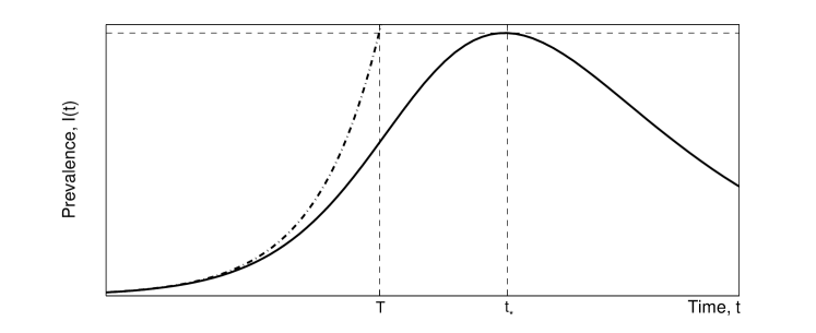
Figure 1: Visualisation of the late time approximation. Peak time $t_{*}$ corresponds to the peak of the full epidemic (solid black line) and late time $T$ is the equivalent timescale for the exponential growth approximation (dashed line).

This definition makes sense since if the population is initially entirely susceptible we may approximate $S(t)\approx 1-\varepsilon{\rm e}^{\lambda t}$. The time at which this quantity first exceeds $1/R_{0}$ should therefore correspond to a sensible definition of late time. Figure 1 visualises the concepts involved in this definition.

3.4 Separation of early and late time

We are now in a position to compare early and late time. Clearly, it is always possible to make $\varepsilon$ sufficiently small to keep these timescales separated; explicitly, this requires

$$\tau\ll T\quad\Rightarrow\quad\varepsilon\ll\frac{R_{0}-1}{R_{0}}\;\mathrm{exp}\left(\frac{\lambda}{\tilde{\lambda}-\lambda}\right)\text{ .}$$ (3.4)

Now suppose we consider transmission based on a Basic Mixing Matrix multiplied by an overall transmission rate $\nu$ so that $\mathbf{M}=\nu\mathbf{B}(\alpha,n)$, meaning that the eigensystem of $\mathbf{M}-\mathbf{G}$ can be obtained by application of Theorem 3. The basic reproductive ratio is $R_{0}=\nu(n+\alpha)/\gamma$, and for an initial infection of $I_{0}$ in the $i^{th}$ age group,

$$\mathbf{I}(0)=(0,\ldots,0,\underbracket{I_{0}}_{\mathclap{i\text{-th position}}},0,\ldots,0)^{\top}=\frac{I_{0}}{n}\ (\mathbf{v}_{1}-\mathbf{v}_{i})\text{ .}$$ (3.5)

Note that the symmetry of the system means that we can let $i\neq 1$ without loss of generality. This initial condition leads to early behaviour

$$\mathbf{I}(t)=\frac{I_{0}}{n}{\rm e}^{\lambda t}\left(\mathbf{v}_{1}-{\rm e}^{-(\lambda-\tilde{\lambda})t}\mathbf{v}_{i}\right)\text{ ,}\quad\text{where}\quad\lambda=\nu(n+\alpha)-\gamma\text{ ,}\quad\tilde{\lambda}=\nu\alpha-\gamma\text{ ,}\quad$$ (3.6)

and so the early time $\tau=1/(\nu n)$ . It is most instructive to consider what happens at constant $R_{0}$, so substituting into (3.4) in this regime gives separation of timescales when

$$I_{0}\ll\frac{R_{0}-1}{R_{0}}\mathrm{exp}\left(\frac{R_{0}-1}{(\nu\alpha/\gamma)-R_{0}}\right)\text{ .}$$ (3.7)

Taking appropriate partial derivatives of the right-hand side of this expression, we see that for a given $R_{0}$, a lower $I_{0}$ is required to secure convergence if we increase $\nu$ or $\alpha$, or if we decrease $\gamma$. This is as would be expected from thinking qualitatively about the problem.

4 Numerical approach

4.1 Quantification of convergence

It will be convenient to define a numerical measure $\phi(t)$ of convergence to the dominant eigenvalue.

$$\phi(t) \coloneqq\mathrm{tan}^{-1}(\psi(t))\text{ ,}$$ (4.1)

$$\text{where}\qquad\psi(t) \coloneqq\frac{{\rm d}}{{\rm d}t}\left(\mathrm{ln}\left(\frac{I(t)}{J(t)}\right)\right)\text{ ,}$$

$$I(t) \coloneqq\sum_{a}I_{a}(t)\text{ ,}$$

$$J(t) \coloneqq{\rm e}^{\lambda t}\text{ .}$$

This definition gives $\phi(t)=0$ at times when the epidemic moves along the dominant eigenvector, and non-zero values in the interval $(-1,1)$ otherwise.

4.2 Contact survey data

We take the form for $\mathbf{M}$ in our numerical work from the results of the POLYMOD study (Mossong et al., 2008) for all reported contacts (physical and conversational) across all countries. We use age classes of width 5 years and a final class for ages 70+. Consideration of population pyramids (Wroth and Wiles, 2009; Stillwell and Clarke, 2011) shows that each age group is of almost equal weighting up to 70, after which the rest of the population is in a rapidly declining tail which in total is roughly equal to the weighting of one of the 5 year classes, and so for present purposes where we are looking for broad insights rather than precise predictions the normalisation (2.2) is appropriate.

4.3 Results

When we integrate (2.1) directly using Runge-Kutta, for infection starting in the 15–19 age group, Figure 2 shows the results obtained for $\phi(t)$ and $I(t)$. Strikingly, this plot shows that even during periods of the epidemic where the prevalence timeseries looks linear on a logarithmic y-axis, $\phi(t)$ can fail to equal zero for an appreciable period of time (meaning that the dynamics (2.1) are not governed by the dominant eigenvector) for modest initial infectious populations. Whether such initial concentrations of infection can be seen, perhaps as a result of an unpredictable event early in the epidemic when stochastic effects dominate, depends on the population size that can be seen as mixing according to (2.1). At country size – i.e. tens or hundreds of millions of individuals – small $I_{0}$ is most likely, but at city sizes of around $10^{5}$, it is not inconceivable that an epidemic could start with several hundred students in the same school leading to $I_{0}\sim 10^{-3}$.

5 Discussion

In this paper, we have considered the real-time rate of convergence of age-structured SIR epidemic models to their dominant eigenvector, both analytically for a basic model of assortative mixing, and numerically for realistic mixing. In each case, sufficiently small initially infectious populations are needed to ensure that the dynamical system does indeed converge before the depletion of susceptibles becomes important. In many cases this effect will not matter; but it is plausible that for some supercritical epidemics in moderately-sized, closed populations with strongly age-structured mixing, this failure of convergence to the dominant eigenvector will be a source of bias. In particular, attempts to infer the relative susceptibility of different age classes may become biased. If a particular age group is over-represented in the initially infected group as compared to the dominant eigenvector, then its relative susceptibility may be overestimated. Correction for non-convergence to the dominant eigenvector is therefore potentially important in epidemiological analysis.

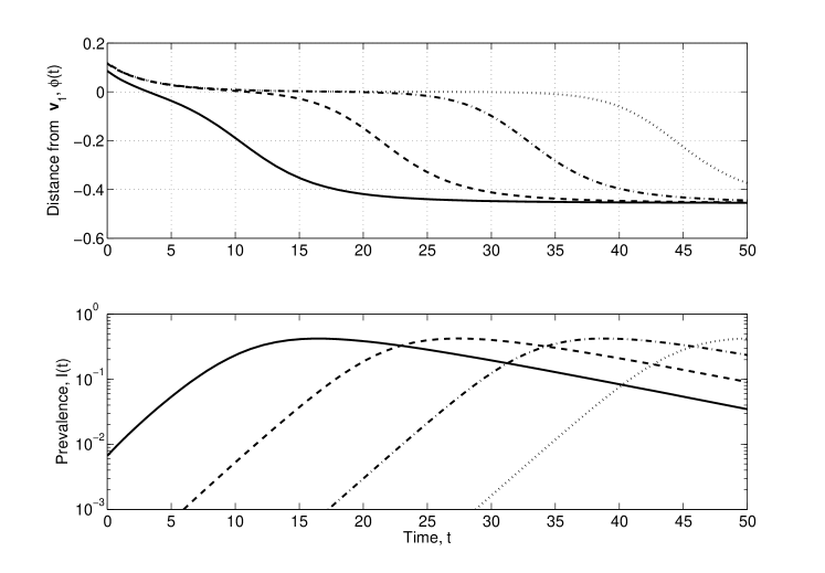
Figure 2: Top: Distance from the dominant eigenvalue, $\phi$, for the POLYMOD mixing matrix. Bottom: prevalence against time on a logarithmic scale. Parameters are: $R_{0}=5$, $\gamma=0.1$, $I_{0}=10^{-1}$ (solid lines), $I_{0}=10^{-3}$ (dashed lines), $I_{0}=10^{-5}$ (dash-dot lines), $I_{0}=10^{-7}$ (dotted lines). Infection is started in the 15–19 year-old age group.

References

- Anderson and May (1983) R. M. Anderson and R. M. May. Vaccination against rubella and measles: quantitative investigations of different policies. The Journal of Hygiene, 90(2):259–325, 1983.
- Anderson and May (1991) R. M. Anderson and R. M. May. Infectious Diseases of Humans. Oxford University Press, Oxford, England, 1991.
- Baguelin et al. (2010) M. Baguelin, A. J. van Hoek, M. Jit, S. Flasche, P. White, and W. J. Edmunds. Vaccination against pandemic influenza A/H1N1v in England: a real-time economic evaluation. Vaccine, 28:12(2370-2384), 2010.
- del Valle et al. (2007) S. Y. del Valle, J. M. Hyman, H. W. Hethcote, and S. G. Eubank. Mixing patterns between age groups in social networks. Social Networks, 29(4):539–554, 2007.
- Diekmann and Heesterbeek (2000) O. Diekmann and J. A. P. Heesterbeek. Mathematical Epidemiology of Infectious Diseases: Model Building, Analysis and Interpretation. John Wiley and Sons Ltd, Chichester, West Sussex, England, 2000.
- Diekmann et al. (1990) O. Diekmann, J. A. P. Heesterbeek, and J. A. J. Metz. On the definition and the computation of the basic reproduction ratio in models for infectious diseases in heterogeneous populations. Journal of Mathematical Biology, 28(4):365–382, Jan 1990.
- Edmunds et al. (2006) W. Edmunds, G. Kafatos, J. Wallinga, and J. Mossong. Mixing patterns and the spread of close-contact infectious diseases. Emerging Themes in Epidemiology, 3(909-912), 2006.
- Glasser et al. (2012) J. Glasser, Z. Feng, A. Moylan, S. Y. del Valle, and C. Castillo-Chavez. Mixing in age-structured population models of infectious diseases. Mathematical Biosciences, 235, 2012.
- Keeling and Rohani (2008) M. J. Keeling and P. Rohani. Modeling Infectious Diseases in Humans and Animals. Princeton University Press, Princeton, New Jersey, USA, 2008.
- Meyer (2000) C. D. Meyer. Matrix Analysis and Applied Linear Algebra. SIAM, Philadelphia, USA, 2000.
- Mossong et al. (2008) J. Mossong, N. Hens, M. Jit, P. Beutels, K. Auranen, R. Mikolajczyk, M. Massari, S. Salmaso, G. S. Tomba, J. Wallinga, J. Heijne, M. Sadkowska-Todys, M. Rosinska, and W. J. Edmunds. Social contacts and mixing patterns relevant to the spread of infectious diseases. PLoS Medicine, 5(3):e74, 2008.
- Stillwell and Clarke (2011) J. Stillwell and M. Clarke. Population Dynamics and Projection Methods. Springer Netherlands, Dordrecht Netherlands, 2011.
- Tuljapurkar (1982) S. D. Tuljapurkar. Why use population entropy? It determines the rate of convergence. Journal of Mathematical Biology, 13:325–337, 1982.
- Wroth and Wiles (2009) E. C. Wroth and A. Wiles. Key population and vital statistics. 2007 data. Office for National Statistics, 34, 2009.