Improving CUR Matrix Decomposition and the Nyström Approximation via Adaptive Sampling

Abstract

The CUR matrix decomposition and the Nyström approximation are two important low-rank matrix approximation techniques. The Nyström method approximates a symmetric positive semidefinite matrix in terms of a small number of its columns, while CUR approximates an arbitrary data matrix by a small number of its columns and rows. Thus, CUR decomposition can be regarded as an extension of the Nyström approximation.

In this paper we establish a more general error bound for the adaptive column/row sampling algorithm, based on which we propose more accurate CUR and Nyström algorithms with expected relative-error bounds. The proposed CUR and Nyström algorithms also have low time complexity and can avoid maintaining the whole data matrix in RAM. In addition, we give theoretical analysis for the lower error bounds of the standard Nyström method and the ensemble Nyström method. The main theoretical results established in this paper are novel, and our analysis makes no special assumption on the data matrices.

Keywords: large-scale matrix computation, CUR matrix decomposition, the Nyström method, randomized algorithms, adaptive sampling

1 Introduction

Large-scale matrices emerging from stocks, genomes, web documents, web images and videos everyday bring new challenges in modern data analysis. Most efforts have been focused on manipulating, understanding and interpreting large-scale data matrices. In many cases, matrix factorization methods are employed for constructing parsimonious and informative representations to facilitate computation and interpretation. A principled approach is the truncated singular value decomposition (SVD) which finds the best low-rank approximation of a data matrix. Applications of SVD such as eigenfaces (Sirovich and Kirby, 1987; Turk and Pentland, 1991) and latent semantic analysis (Deerwester et al., 1990) have been illustrated to be very successful.

However, using SVD to find basis vectors and low-rank approximations has its limitations. As pointed out by Berry et al. (2005), it is often useful to find a low-rank matrix approximation which posses additional structures such as sparsity or nonnegativity. Since SVD or the standard QR decomposition for sparse matrices does not preserve sparsity in general, when the sparse matrix is large, computing or even storing such decompositions becomes challenging. Therefore it is useful to compute a low-rank matrix decomposition which preserves such structural properties of the original data matrix.

Another limitation of SVD is that the basis vectors resulting from SVD have little concrete meaning, which makes it very difficult for us to understand and interpret the data in question. An example of Drineas et al. (2008) and Mahoney and Drineas (2009) has well shown this viewpoint; that is, the vector $[(1/2)\textrm{age}-(1/\sqrt{2})\textrm{height}+(1/2)\textrm{income}]$, the sum of the significant uncorrelated features from a data set of people’s features, is not particularly informative. Kuruvilla et al. (2002) have also claimed: “it would be interesting to try to find basis vectors for all experiment vectors, using actual experiment vectors and not artificial bases that offer little insight.” Therefore, it is of great interest to represent a data matrix in terms of a small number of actual columns and/or actual rows of the matrix. Matrix column selection and the CUR matrix decomposition provide such techniques.

1.1 Matrix Column Selection

Column selection has been extensively studied in the theoretical computer science (TCS) and numerical linear algebra (NLA) communities. The work in TCS mainly focuses on choosing good columns by randomized algorithms with provable error bounds (Frieze et al., 2004; Deshpande et al., 2006; Drineas et al., 2008; Deshpande and Rademacher, 2010; Boutsidis et al., 2011; Guruswami and Sinop, 2012). The focus in NLA is then on deterministic algorithms, especially the rank-revealing QR factorizations, that select columns by pivoting rules (Foster, 1986; Chan, 1987; Stewart, 1999; Bischof and Hansen, 1991; Hong and Pan, 1992; Chandrasekaran and Ipsen, 1994; Gu and Eisenstat, 1996; Berry et al., 2005). In this paper we focus on randomized algorithms for column selection.

Given a matrix ${\bf A}\in{{\mathbb{R}}^{m\times n}}$, column selection algorithms aim to choose $c$ columns of ${\bf A}$ to construct a matrix ${\bf C}\in{\mathbb{R}}^{m\times c}$ such that $\|{\bf A}-{\bf C}{{\bf C}^{{\dagger}}}{\bf A}\|_{\xi}$ achieves the minimum. Here “$\xi=2$,” “$\xi=F$,” and “$\xi=*$” respectively represent the matrix spectral norm, the matrix Frobenius norm, and the matrix nuclear norm, and ${{\bf C}^{{\dagger}}}$ denotes the Moore-Penrose inverse of ${\bf C}$. Since there are $(^{n}_{c})$ possible choices of constructing ${\bf C}$, selecting the best subset is a hard problem.

In recent years, many polynomial-time approximate algorithms have been proposed. Among them we are especially interested in those algorithms with multiplicative upper bounds; that is, there exists a polynomial function $f(m,n,k,c)$ such that with $c$ $(\geq k)$ columns selected from ${\bf A}$ the following inequality holds

$$\|{\bf A}-{\bf C}{{\bf C}^{{\dagger}}}{\bf A}\|_{\xi}\;\leq\;f(m,n,k,c)\,\|{\bf A}-{\bf A}_{k}\|_{\xi}$$

with high probability (w.h.p.) or in expectation w.r.t. ${\bf C}$. We call $f$ the approximation factor. The bounds are strong when $f=1+\epsilon$ for an error parameter $\epsilon$—they are known as relative-error bounds. Particularly, the bounds are called constant-factor bounds when $f$ does not depend on $m$ and $n$ (Mahoney, 2011). The relative-error bounds and constant-factor bounds of the CUR matrix decomposition and the Nyström approximation are similarly defined.

However, the column selection method, also known as the ${\bf A}\approx{\bf C}{\bf X}$ decomposition in some applications, has its limitations. For a large sparse matrix ${\bf A}$, its submatrix ${\bf C}$ is sparse, but the coefficient matrix ${\bf X}\in{\mathbb{R}}^{c\times n}$ is not sparse in general. The ${\bf C}{\bf X}$ decomposition suffices when $m\gg n$, because ${\bf X}$ is small in size. However, when $m$ and $n$ are near equal, computing and storing the dense matrix ${\bf X}$ in RAM becomes infeasible. In such an occasion the CUR matrix decomposition is a very useful alternative.

1.2 The CUR Matrix Decomposition

The CUR matrix decomposition problem has been widely discussed in the literature (Goreinov et al., 1997a, b; Stewart, 1999; Tyrtyshnikov, 2000; Berry et al., 2005; Drineas and Mahoney, 2005; Mahoney et al., 2008; Bien et al., 2010), and it has been shown to be very useful in high dimensional data analysis. Particularly, a CUR decomposition algorithm seeks to find a subset of $c$ columns of ${\bf A}$ to form a matrix ${\bf C}\in{\mathbb{R}}^{m{\times}c}$, a subset of $r$ rows to form a matrix ${\bf R}\in{\mathbb{R}}^{r{\times}n}$, and an intersection matrix ${\bf U}\in{\mathbb{R}}^{c{\times}r}$ such that $\|{\bf A}-{\bf C}{\bf U}{\bf R}\|_{\xi}$ is small. Accordingly, we use $\tilde{{\bf A}}={\bf C}{\bf U}{\bf R}$ to approximate ${\bf A}$.

Drineas et al. (2006) proposed a CUR algorithm with additive-error bound. Later on, Drineas et al. (2008) devised a randomized CUR algorithm which has relative-error bound w.h.p. if sufficiently many columns and rows are sampled. Mackey et al. (2011) established a divide-and-conquer method which solves the CUR problem in parallel. The CUR algorithms guaranteed by relative-error bounds are of great interest.

Unfortunately, the existing CUR algorithms usually require a large number of columns and rows to be chosen. For example, for an $m{\times}n$ matrix ${\bf A}$ and a target rank $k\ll\min\{m,n\}$, the subspace sampling algorithm (Drineas et al., 2008)—a classical CUR algorithm—requires ${\mathcal{O}}(k\epsilon^{-2}\log k)$ columns and ${\mathcal{O}}(k\epsilon^{-4}\log^{2}k)$ rows to achieve relative-error bound w.h.p. The subspace sampling algorithm selects columns/rows according to the statistical leverage scores, so the computational cost of this algorithm is at least equal to the cost of the truncated SVD of ${\bf A}$, that is, ${\mathcal{O}}(mnk)$ in general. However, maintaining a large scale matrix in RAM is often impractical, not to mention performing SVD. Recently, Drineas et al. (2012) devised fast approximation to statistical leverage scores which can be used to speedup the subspace sampling algorithm heuristically—yet no theoretical results have been reported that the leverage scores approximation can give provably efficient subspace sampling algorithm.

The CUR matrix decomposition problem has a close connection with the column selection problem. Especially, most CUR algorithms such as those of Drineas and Kannan (2003); Drineas et al. (2006, 2008) work in a two-stage manner where the first stage is a standard column selection procedure. Despite their strong resemblance, CUR is a harder problem than column selection because “one can get good columns or rows separately” does not mean that one can get good columns and rows together. If the second stage is naïvely solved by a column selection algorithm on ${\bf A}^{T}$, then the approximation factor will trivially be $\sqrt{2}f$ (Mahoney and Drineas, 2009). Thus, more sophisticated error analysis techniques for the second stage are indispensable in order to achieve relative-error bound.

1.3 The Nyström Methods

The Nyström approximation is closely related to CUR, and it can potentially benefit from the advances in CUR techniques. Different from CUR, the Nyström methods are used for approximating symmetric positive semidefinite (SPSD) matrices. The methods approximate an SPSD matrix only using a subset of its columns, so they can alleviate computation and storage costs when the SPSD matrix in question is large in size. In fact, the Nyström methods have been extensively used in the machine learning community. For example, they have been applied to Gaussian processes (Williams and Seeger, 2001), kernel SVMs (Zhang et al., 2008), spectral clustering (Fowlkes et al., 2004), kernel PCA (Talwalkar et al., 2008; Zhang et al., 2008; Zhang and Kwok, 2010), etc.

The Nyström methods approximate any SPSD matrix in terms of a subset of its columns. Specifically, given an $m{\times}m$ SPSD matrix ${{\bf A}}$, they require sampling $c$ ($<m$) columns of ${{\bf A}}$ to construct an $m\times c$ matrix ${{\bf C}}$. Since there exists an $m{\times}m$ permutation matrix $\Pi$ such that $\mbox{\boldmath$\Pi$\unboldmath}{{\bf C}}$ consists of the first $c$ columns of $\mbox{\boldmath$\Pi$\unboldmath}{{\bf A}}\mbox{\boldmath$\Pi$\unboldmath}^{T}$, we always assume that ${{\bf C}}$ consists of the first $c$ columns of ${\bf A}$ without loss of generality. We partition ${\bf A}$ and ${\bf C}$ as

$${\bf A}\;=\;\begin{bmatrix}{\bf W}&{\bf A}_{21}^{T}\\ {\bf A}_{21}&{\bf A}_{22}\end{bmatrix}\quad\textrm{ and }\quad{\bf C}\;=\;\begin{bmatrix}{\bf W}\\ {\bf A}_{21}\end{bmatrix}\textrm{,}$$

where ${\bf W}$ and ${\bf A}_{21}$ are of sizes $c\times c$ and $(m{-}c)\times c$, respectively. There are three models which are defined as follows.

• The Standard Nyström Method. The standard Nyström approximation to ${\bf A}$ is

  $$\tilde{{\bf A}}_{c}^{\textrm{nys}}\;=\;{\bf C}{\bf W}^{\dagger}{\bf C}^{T}\;=\;\left[\begin{array}[]{cc}{\bf W}&{\bf A}_{21}^{T}\\ {\bf A}_{21}&{\bf A}_{21}{\bf W}^{\dagger}{\bf A}_{21}^{T}\\ \end{array}\right]\textrm{.}$$ (1)

  Here ${\bf W}^{\dagger}$ is called the intersection matrix. The matrix $({\bf W}_{k})^{\dagger}$, where $k\leq c$ and ${\bf W}_{k}$ is the best $k$-rank approximation to ${\bf W}$, is also used as an intersection matrix for constructing approximations with even lower rank. But using ${\bf W}^{\dagger}$ results in a tighter approximation than using $({\bf W}_{k})^{\dagger}$ usually.

• The Ensemble Nyström Method (Kumar et al., 2009). It selects a collection of $t$ samples, each sample ${{\bf C}^{(i)}}$, ($i=1,\cdots,t$), containing $c$ columns of ${\bf A}$. Then the ensemble method combines the samples to construct an approximation in the form of

  $$\tilde{{\bf A}}_{t,c}^{\textrm{ens}}\;=\;\sum_{i=1}^{t}\mu^{(i)}{{\bf C}^{(i)}}{{\bf W}^{(i)}}^{\dagger}{{\bf C}^{(i)}}^{T}\textrm{,}$$ (2)

  where $\mu^{(i)}$ are the weights of the samples. Typically, the ensemble Nyström method seeks to find out the weights by minimizing $\|{\bf A}-\tilde{{\bf A}}_{t,c}^{\textrm{ens}}\|_{F}$ or $\|{\bf A}-\tilde{{\bf A}}_{t,c}^{\textrm{ens}}\|_{2}$. A simple but effective strategy is to set the weights as $\mu^{(1)}=\cdots=\mu^{(t)}=\frac{1}{t}$.

• The Modified Nyström Method (proposed in this paper). It is defined as

  $$\tilde{{\bf A}}_{c}^{\textrm{mod}}\;=\;{\bf C}\big{(}{\bf C}^{\dagger}{\bf A}({\bf C}^{\dagger})^{T}\big{)}{\bf C}^{T}.$$

  This model is not strictly the Nyström method because it uses a quite different intersection matrix ${\bf C}^{\dagger}{\bf A}({\bf C}^{\dagger})^{T}$. It costs ${\mathcal{O}}(mc^{2})$ time to compute the Moore-Penrose inverse ${\bf C}^{\dagger}$ and $m^{2}c$ flops to compute matrix multiplications. The matrix multiplications can be executed very efficiently in multi-processor environment, so ideally computing the intersection matrix costs time only linear in $m$. This model is more accurate (which will be justified in Section 4.3 and 4.4) but more costly than the conventional ones, so there is a trade-off between time and accuracy when deciding which model to use.

Here and later, we call those which use intersection matrix ${\bf W}^{\dagger}$ or $({\bf W}_{k})^{\dagger}$ the conventional Nyström methods, including the standard Nyström and the ensemble Nyström.

To generate effective approximations, much work has been built on the upper error bounds of the sampling techniques for the Nyström method. Most of the work, for example, Drineas and Mahoney (2005), Li et al. (2010), Kumar et al. (2009), Jin et al. (2011), and Kumar et al. (2012), studied the additive-error bound. With assumptions on matrix coherence, better additive-error bounds were obtained by Talwalkar and Rostamizadeh (2010), Jin et al. (2011), and Mackey et al. (2011). However, as stated by Mahoney (2011), additive-error bounds are less compelling than relative-error bounds. In one recent work, Gittens and Mahoney (2013) provided a relative-error bound for the first time, where the bound is in nuclear norm.

However, the error bounds of the previous Nyström methods are much weaker than those of the existing CUR algorithms, especially the relative-error bounds in which we are more interested (Mahoney, 2011). Actually, as will be proved in this paper, the lower error bounds of the standard Nyström method and the ensemble Nyström method are even much worse than the upper bounds of some existing CUR algorithms. This motivates us to improve the Nyström method by borrowing the techniques in CUR matrix decomposition.

1.4 Contributions and Outline

The main technical contribution of this work is the adaptive sampling bound in Theorem 5, which is an extension of Theorem 2.1 of Deshpande et al. (2006). Theorem 2.1 of Deshpande et al. (2006) bounds the error incurred by projection onto column or row space, while our Theorem 5 bounds the error incurred by the projection simultaneously onto column space and row space. We also show that Theorem 2.1 of Deshpande et al. (2006) can be regarded as a special case of Theorem 5.

More importantly, our adaptive sampling bound provides an approach for improving CUR and the Nyström approximation: no matter which relative-error column selection algorithm is employed, Theorem 5 ensures relative-error bounds for CUR and the Nyström approximation. We present the results in Corollary 7.

Based on the adaptive sampling bound in Theorem 5 and its corollary 7, we provide a concrete CUR algorithm which beats the best existing algorithm—the subspace sampling algorithm—both theoretically and empirically. The CUR algorithm is described in Algorithm 2 and analyzed in Theorem 8. In Table 1 we present a comparison between our proposed CUR algorithm and the subspace sampling algorithm. As we see, our algorithm requires much fewer columns and rows to achieve relative-error bound. Our method is more scalable for it works on only a few columns or rows of the data matrix in question; in contrast, the subspace sampling algorithm maintains the whole data matrix in RAM to implement SVD.

	#column ($c$)	#row ($r$)	time	space
Adaptive	$\frac{2k}{\epsilon}\big{(}1+o(1)\big{)}$	$\frac{c}{\epsilon}\big{(}1+\epsilon\big{)}$	Roughly ${\mathcal{O}}\big{(}nk^{2}\epsilon^{-4}\big{)}+{T_{\mathrm{Multiply}}}\big{(}mnk\epsilon^{-1}\big{)}$	${\mathcal{O}}\big{(}\max\{mc,nr\}\big{)}$
Subspace	${\mathcal{O}}\Big{(}\frac{k\log k}{\epsilon^{2}}\Big{)}$	${\mathcal{O}}\Big{(}\frac{c\log c}{\epsilon^{2}}\Big{)}$	${\mathcal{O}}\big{(}mnk\big{)}$	${\mathcal{O}}(mn)$

Table 1: Comparisons between our adaptive sampling based CUR algorithm and the best existing algorithm—the subspace sampling algorithm of Drineas et al. (2008).

Another important application of the adaptive sampling bound is to yield an algorithm for the modified Nyström method. The algorithm has a strong relative-error upper bound: for a target rank $k$, by sampling $\frac{2k}{\epsilon^{2}}\big{(}1+o(1)\big{)}$ columns it achieves relative-error bound in expectation. The results are shown in Theorem 10.

Finally, we establish a collection of lower error bounds of the standard Nyström and the ensemble Nyström that use ${\bf W}^{\dagger}$ as the intersection matrix. We show the lower bounds in Theorem 12 and Table 3; here Table 2 briefly summarizes the lower bounds in Table 3. From the table we can see that the upper error bound of our adaptive sampling algorithm for the modified Nyström method is even better than the lower bounds of the conventional Nyström methods.

	$\frac{\|{\bf A}-\tilde{{\bf A}}\|_{F}}{\max_{i,j}|a_{ij}|}$	$\frac{\|{\bf A}-\tilde{{\bf A}}\|_{2}}{\max_{i,j}|a_{ij}|}$	$\frac{\|{\bf A}-\tilde{{\bf A}}\|_{*}}{\max_{i,j}|a_{ij}|}$	$\frac{\|{\bf A}-\tilde{{\bf A}}\|_{F}}{\|{\bf A}-{\bf A}_{k}\|_{F}}$	$\frac{\|{\bf A}-\tilde{{\bf A}}\|_{2}}{\|{\bf A}-{\bf A}_{k}\|_{2}}$	$\frac{\|{\bf A}-\tilde{{\bf A}}\|_{*}}{\|{\bf A}-{\bf A}_{k}\|_{*}}$
Standard	$\Omega\big{(}\frac{m\sqrt{k}}{c}\big{)}$	$\Omega\big{(}\frac{{m}}{c}\big{)}$	$\Omega\big{(}m-c\big{)}$	$\Omega\Big{(}\sqrt{1+\frac{mk}{c^{2}}}\Big{)}$	$\Omega\big{(}\frac{m}{c}\big{)}$	$\Omega\big{(}1+\frac{k}{c}\big{)}$
Ensemble	$\Omega\big{(}\frac{{m\sqrt{k}}}{c}\big{)}$	–	$\Omega\big{(}m-c\big{)}$	$\Omega\Big{(}\sqrt{1+\frac{mk}{c^{2}}}\Big{)}$	–	$\Omega\big{(}1+\frac{k}{c}\big{)}$

Table 2: Lower bounds of the standard Nyström method and the ensemble Nyström method. The blanks indicate the lower bounds are unknown to us. Here $m$ denotes the column/row number of the SPSD matrix, $c$ denotes the number of selected columns, and $k$ denotes the target rank.

The remainder of the paper is organized as follows. In Section 2 we give the notation that will be used in this paper. In Section 3 we survey the previous work on the randomized column selection, CUR matrix decomposition, and Nyström approximation. In Section 4 we present our theoretical results and corresponding algorithms. In Section 5 we empirically evaluate our proposed CUR and Nyström algorithms. Finally, we conclude our work in Section 6. All proofs are deferred to the appendices.

2 Notation

First of all, we present the notation and notion that are used here and later. We let ${\bf I}_{m}$ denote the $m\times m$ identity matrix, ${\bf 1}_{m}$ denote the $m{\times}1$ vector of ones, and ${\bf 0}$ denote a zero vector or matrix with appropriate size. For a matrix ${\bf A}=[a_{ij}]\in{\mathbb{R}}^{m\times n}$, we let ${\bf a}^{(i)}$ be its $i$-th row, ${\bf a}_{j}$ be its $j$-th column, and ${\bf A}_{i:j}$ be a submatrix consisting of its $i$ to $j$-th columns ($i\leq j$).

Let $\rho=\mathrm{rank}({\bf A})\leq\min\{m,n\}$ and $k\leq\rho$. The singular value decomposition (SVD) of ${\bf A}$ can be written as

$${\bf A}=\sum_{i=1}^{\rho}\sigma_{{\bf A},i}{\bf u}_{{\bf A},i}{\bf v}^{T}_{{\bf A},i}={{{\bf U}}_{{\bf A}}}{{\mbox{\boldmath$\Sigma$\unboldmath}}_{{\bf A}}}{\bf V}_{{\bf A}}^{T}=\left[\begin{array}[]{cc}{{{\bf U}}_{{\bf A},k}}&{{{\bf U}}_{{\bf A},k\perp}}\\ \end{array}\right]\left[\begin{array}[]{cc}{{\mbox{\boldmath$\Sigma$\unboldmath}}_{{\bf A},k}}&{\bf 0}\\ {\bf 0}&{{\mbox{\boldmath$\Sigma$\unboldmath}}_{{\bf A},k\perp}}\\ \end{array}\right]\left[\begin{array}[]{c}{\bf V}_{{\bf A},k}^{T}\\ {\bf V}_{{\bf A},k\perp}^{T}\\ \end{array}\right]\textrm{,}$$

where ${{{\bf U}}_{{\bf A},k}}$ ($m{\times}k$), ${{\mbox{\boldmath$\Sigma$\unboldmath}}_{{\bf A},k}}$ ($k{\times}k$), and ${{{\bf V}}_{{\bf A},k}}$ ($n{\times}k$) correspond to the top $k$ singular values. We denote ${\bf A}_{k}={{{\bf U}}_{{\bf A},k}}{{\mbox{\boldmath$\Sigma$\unboldmath}}_{{\bf A},k}}{\bf V}_{{\bf A},k}^{T}$ which is the best (or closest) rank-$k$ approximation to ${\bf A}$. We also use $\sigma_{i}({\bf A})=\sigma_{{\bf A},i}$ to denote the $i$-th largest singular value. When ${\bf A}$ is SPSD, the SVD is identical to the eigenvalue decomposition, in which case we have ${{{\bf U}}_{{\bf A}}}={{{\bf V}}_{{\bf A}}}$.

We define the matrix norms as follows. Let $\|{\bf A}\|_{1}=\sum_{i,j}|a_{ij}|$ be the $\ell_{1}$-norm, $\|{\bf A}\|_{F}=(\sum_{i,j}a_{ij}^{2})^{1/2}=(\sum_{i}\sigma^{2}_{{\bf A},i})^{1/2}$ be the Frobenius norm, $\|{\bf A}\|_{2}=\max_{{\bf x}\in{\mathbb{R}}^{n},\|{\bf x}\|_{2}=1}\|{\bf A}{\bf x}\|_{2}=\sigma_{{\bf A},1}$ be the spectral norm, and $\|{\bf A}\|_{*}=\sum_{i}\sigma_{{\bf A},i}$ be the nuclear norm. We always use $\|\cdot\|_{\xi}$ to represent $\|\cdot\|_{2}$, $\|\cdot\|_{F}$, or $\|\cdot\|_{*}$.

Based on SVD, the statistical leverage scores of the columns of ${\bf A}$ relative to the best rank-$k$ approximation to ${\bf A}$ is defined as

$$\ell_{j}^{[k]}=\big{\|}{\bf v}_{{\bf A},k}^{(j)}\big{\|}_{2}^{2}\textrm{, }\quad j=1,\cdots,n\textrm{.}$$ (3)

We have that $\sum_{j=1}^{n}\ell_{j}^{[k]}=k$. The leverage scores of the rows of ${\bf A}$ are defined according to ${\bf U}_{{\bf A},k}$. The leverage scores play an important role in low-rank matrix approximation. Informally speaking, the columns (or rows) with high leverage scores have greater influence in rank-$k$ approximation than those with low leverage scores.

Additionally, let ${{\bf A}^{{\dagger}}}={\bf V}_{{\bf A},\rho}\mbox{\boldmath$\Sigma$\unboldmath}_{{\bf A},\rho}^{-1}{\bf U}_{{\bf A},\rho}^{T}$ be the Moore-Penrose inverse of ${\bf A}$ (Ben-Israel and Greville, 2003). When ${\bf A}$ is nonsingular, the Moore-Penrose inverse is identical to the matrix inverse. Given matrices ${\bf A}\in{{\mathbb{R}}^{m\times n}}$, ${\bf X}\in{\mathbb{R}}^{m\times p}$, and ${\bf Y}\in{\mathbb{R}}^{q\times n}$, ${\bf X}{\bf X}^{\dagger}{\bf A}={\bf U}_{\bf X}{\bf U}_{{\bf X}}^{T}{\bf A}\in{{\mathbb{R}}^{m\times n}}$ is the projection of ${\bf A}$ onto the column space of ${\bf X}$, and ${\bf A}{\bf Y}^{\dagger}{\bf Y}={\bf A}{\bf V}_{\bf Y}{\bf V}_{{\bf Y}}^{T}\in{{\mathbb{R}}^{m\times n}}$ is the projection of ${\bf A}$ onto the row space of ${\bf Y}$.

Finally, we discuss the computational costs of the matrix operations mentioned above. For an $m{\times}n$ general matrix ${\bf A}$ (assume $m\geq n$), it takes ${\mathcal{O}}(mn^{2})$ flops to compute the full SVD and ${\mathcal{O}}(mnk)$ flops to compute the truncated SVD of rank $k$ ($<n$). The computation of ${\bf A}^{\dagger}$ also takes ${\mathcal{O}}(mn^{2})$ flops. It is worth mentioning that, although multiplying an $m{\times}n$ matrix by an $n{\times}p$ matrix runs in $mnp$ flops, it can be easily performed in parallel (Halko et al., 2011). In contrast, implementing operations like SVD and QR decomposition in parallel is much more difficult. So we denote the time complexity of such a matrix multiplication by ${T_{\mathrm{Multiply}}}(mnp)$, which can be tremendously smaller than ${\mathcal{O}}(mnp)$ in practice.

3 Previous Work

In Section 3.1 we present an adaptive sampling algorithm and its relative-error bound established by Deshpande et al. (2006). In Section 3.2 we highlight the near-optimal column selection algorithm of Boutsidis et al. (2011) which we will use in our CUR and Nyström algorithms for column/row sampling. In Section 3.3 we introduce two important CUR algorithms. In Section 3.4 we introduce the only known relative-error algorithm for the standard Nyström method.

3.1 The Adaptive Sampling Algorithm

Adaptive sampling is an effective and efficient column sampling algorithm for reducing the error incurred by the first round of sampling. After one has selected a small subset of columns (denoted ${\bf C}_{1}$), an adaptive sampling method is used to further select a proportion of columns according to the residual of the first round, that is, ${\bf A}-{\bf C}_{1}{\bf C}_{1}^{\dagger}{\bf A}$. The approximation error is guaranteed to be decreasing by a factor after the adaptive sampling (Deshpande et al., 2006). We show the result of Deshpande et al. (2006) in the following lemma.

Lemma 1 (The Adaptive Sampling Algorithm)

(Deshpande et al., 2006)   Given a matrix ${\bf A}\in{{\mathbb{R}}^{m\times n}}$, we let ${\bf C}_{1}\in{\mathbb{R}}^{m\times c_{1}}$ consist of $c_{1}$ columns of ${\bf A}$, and define the residual ${\bf B}={\bf A}-{\bf C}_{1}{\bf C}_{1}^{\dagger}{\bf A}$. Additionally, for $i=1,\cdots,n$, we define

$$p_{i}\;=\;\|{\bf b}_{i}\|_{2}^{2}/\|{\bf B}\|_{F}^{2}.$$

We further sample $c_{2}$ columns i.i.d. from ${\bf A}$, in each trial of which the $i$-th column is chosen with probability $p_{i}$. Let ${\bf C}_{2}\in{\mathbb{R}}^{m\times c_{2}}$ contain the $c_{2}$ sampled columns and let ${\bf C}=[{\bf C}_{1},{\bf C}_{2}]\in{\mathbb{R}}^{m\times(c_{1}+c_{2})}$. Then, for any integer $k>0$, the following inequality holds:

$${\mathbb{E}}\|{\bf A}-{\bf C}{{\bf C}^{{\dagger}}}{\bf A}\|_{F}^{2}\;\leq\;\|{\bf A}-{\bf A}_{k}\|_{F}^{2}+\frac{k}{c_{2}}\|{\bf A}-{\bf C}_{1}{\bf C}_{1}^{\dagger}{\bf A}\|_{F}^{2},$$

where the expectation is taken w.r.t. ${\bf C}_{2}$.

We will establish in Theorem 5 a more general and more useful error bound for this adaptive sampling algorithm. It can be shown that Lemma 1 is a special case of Theorem 5.

3.2 The Near-Optimal Column Selection Algorithm

Boutsidis et al. (2011) proposed a relative-error column selection algorithm which requires only $c={2k\epsilon^{-1}}(1{+}o(1))$ columns get selected. Boutsidis et al. (2011) also proved the lower bound of the column selection problem which shows that no column selection algorithm can achieve relative-error bound by selecting less than $c=k\epsilon^{-1}$ columns. Thus this algorithm is near optimal. Though an optimal algorithm recently proposed by Guruswami and Sinop (2012) attains the the lower bound, this algorithm is quite inefficient in comparison with the near-optimal algorithm. So we prefer to use the near-optimal algorithm in our CUR and Nyström algorithms for column/row sampling.

The near-optimal algorithm consists of three steps: the approximate SVD via random projection (Boutsidis et al., 2011; Halko et al., 2011), the dual set sparsification algorithm (Boutsidis et al., 2011), and the adaptive sampling algorithm (Deshpande et al., 2006). We describe the near-optimal algorithm in Algorithm 1 and present the theoretical analysis in Lemma 2.

Lemma 2 (The Near-Optimal Column Selection Algorithm)

Given a matrix ${\bf A}\in{{\mathbb{R}}^{m\times n}}$ of rank $\rho$, a target rank $k$ $(2\leq k<\rho)$, and $0<\epsilon<1$. Algorithm 1 selects

$$c\;=\;\frac{2k}{\epsilon}\Big{(}1+o(1)\Big{)}$$

columns of ${\bf A}$ to form a matrix ${\bf C}\in{\mathbb{R}}^{m\times c}$, then the following inequality holds:

$${\mathbb{E}}\|{\bf A}-{\bf C}{{\bf C}^{{\dagger}}}{\bf A}\|_{F}^{2}\;\leq\;(1+\epsilon)\,\|{\bf A}-{\bf A}_{k}\|_{F}^{2}\textrm{,}$$

where the expectation is taken w.r.t. ${\bf C}$. Furthermore, the matrix ${\bf C}$ can be obtained in ${\mathcal{O}}\big{(}mk^{2}\epsilon^{-4/3}+nk^{3}\epsilon^{-2/3}\big{)}+{T_{\mathrm{Multiply}}}\big{(}mnk\epsilon^{-2/3}\big{)}$ time.

Algorithm 1 The Near-Optimal Column Selection Algorithm of Boutsidis et al. (2011).

1:  Input: a real matrix ${\bf A}\in{{\mathbb{R}}^{m\times n}}$, target rank $k$, error parameter $\epsilon\in(0,1]$, target column number $c=\frac{2k}{\epsilon}\big{(}1+o(1)\big{)}$;

2:  Compute approximate truncated SVD via random projection such that ${\bf A}_{k}\approx\tilde{{\bf U}}_{k}\tilde{\mbox{\boldmath$\Sigma$\unboldmath}}_{k}\tilde{{\bf V}}_{k}$;

3:  Construct ${\mathcal{U}}\leftarrow$ columns of $({\bf A}-\tilde{{\bf U}}_{k}\tilde{\mbox{\boldmath$\Sigma$\unboldmath}}_{k}\tilde{{\bf V}}_{k})$; $\quad{\mathcal{V}}\leftarrow$ columns of $\tilde{{\bf V}}_{k}^{T}$;

4:  Compute ${\bf s}\leftarrow$ Dual Set Spectral-Frobenius Sparsification Algorithm (${\mathcal{U}}$, ${\mathcal{V}}$, $c-2k/\epsilon$);

5:  Construct ${\bf C}_{1}\leftarrow{\bf A}\mathsf{Diag}({\bf s})$, and then delete the all-zero columns;

6:  Residual matrix ${\bf D}\leftarrow{\bf A}-{\bf C}_{1}{\bf C}_{1}^{\dagger}{\bf A}$;

7:  Compute sampling probabilities: $p_{i}=\|{\bf d}_{i}\|_{2}^{2}/\|{\bf D}\|_{F}^{2}$, $i=1,\cdots,n$;

8:  Sampling $c_{2}=2k/\epsilon$ columns from ${\bf A}$ with probability $\{p_{1},\cdots,p_{n}\}$ to construct ${\bf C}_{2}$;

9:  return  ${\bf C}=[{\bf C}_{1},{\bf C}_{2}]$.

This algorithm has the merits of low time complexity and space complexity. None of the three steps—the randomized SVD, the dual set sparsification algorithm, and the adaptive sampling—requires loading the whole of ${\bf A}$ into RAM. All of the three steps can work on only a small subset of the columns of ${\bf A}$. Though a relative-error algorithm recently proposed by Guruswami and Sinop (2012) requires even fewer columns, it is less efficient than the near-optimal algorithm.

3.3 Previous Work in CUR Matrix Decomposition

We introduce in this section two highly effective CUR algorithms: one is deterministic and the other is randomized.

3.3.1 The Sparse Column-Row Approximation (SCRA)

Stewart (1999) proposed a deterministic CUR algorithm and called it the sparse column-row approximation (SCRA). SCRA is based on the truncated pivoted QR decomposition via a quasi Gram-Schmidt algorithm. Given a matrix ${\bf A}\in{\mathbb{R}}^{m\times n}$, the truncated pivoted QR decomposition procedure deterministically finds a set of columns ${\bf C}\in{\mathbb{R}}^{m\times c}$ by column pivoting, whose span approximates the column space of ${\bf A}$, and computes an upper triangular matrix ${\bf T}_{\bf C}\in{\mathbb{R}}^{c\times c}$ that orthogonalizes those columns. SCRA runs the same procedure again on ${\bf A}^{T}$ to select a set of rows ${\bf R}\in{\mathbb{R}}^{r\times n}$ and computes the corresponding upper triangular matrix ${\bf T}_{\bf R}\in{\mathbb{R}}^{r\times r}$. Let ${\bf C}={\bf Q}_{\bf C}{\bf T}_{\bf C}$ and ${\bf R}^{T}={\bf Q}_{\bf R}{\bf T}_{\bf R}$ denote the resulting truncated pivoted QR decomposition. The intersection matrix is computed by ${\bf U}=({\bf T}_{\bf C}^{T}{\bf T}_{\bf C})^{-1}{\bf C}^{T}{\bf A}{\bf R}^{T}({\bf T}_{\bf R}^{T}{\bf T}_{\bf R})^{-1}$. According to our experiments, this algorithm is quite effective but very time expensive, especially when $c$ and $r$ are large. Moreover, this algorithm does not have data-independent error bound.

3.3.2 The Subspace Sampling CUR Algorithm

Drineas et al. (2008) proposed a two-stage randomized CUR algorithm which has a relative-error bound with high probability (w.h.p.). In the first stage the algorithm samples $c$ columns of ${\bf A}$ to construct ${\bf C}$, and in the second stage it samples $r$ rows from ${\bf A}$ and ${\bf C}$ simultaneously to construct ${\bf R}$ and ${\bf W}$ and let ${\bf U}={\bf W}^{\dagger}$. The sampling probabilities in the two stages are proportional to the leverage scores of ${\bf A}$ and ${\bf C}$, respectively. That is, in the first stage the sampling probabilities are proportional to the squared $\ell_{2}$-norm of the rows of ${\bf V}_{{\bf A},k}$; in the second stage the sampling probabilities are proportional to the squared $\ell_{2}$-norm of the rows of ${\bf U}_{{\bf C}}$. That is why it is called the subspace sampling algorithm. Here we show the main results of the subspace sampling algorithm in the following lemma.

Lemma 3 (Subspace Sampling for CUR )

Given an ${m\times n}$ matrix ${\bf A}$ and a target rank $k\ll\min\{m,n\}$, the subspace sampling algorithm selects $c={\mathcal{O}}(k\epsilon^{-2}\log k\log(1/\delta))$ columns and $r=$ ${\mathcal{O}}\big{(}c\epsilon^{-2}\log c\log(1/\delta)\big{)}$ rows without replacement. Then

$$\|{\bf A}-{\bf C}{\bf U}{\bf R}\|_{F}\;=\;\big{\|}{\bf A}-{\bf C}{\bf W}^{\dagger}{\bf R}\big{\|}_{F}\;\leq\;(1+\epsilon)\|{\bf A}-{\bf A}_{k}\|_{F}\textrm{,}$$

holds with probability at least $1-\delta$, where ${\bf W}$ contains the rows of ${\bf C}$ with scaling. The running time is dominated by the truncated SVD of ${\bf A}$, that is, ${\mathcal{O}}(mnk)$.

3.4 Previous Work in the Nyström Approximation

In a very recent work, Gittens and Mahoney (2013) established a framework for analyzing errors incurred by the standard Nyström method. Especially, the authors provided the first and the only known relative-error (in nuclear norm) algorithm for the standard Nyström method. The algorithm is described as follows and, its bound is shown in Lemma 4.

Like the CUR algorithm in Section 3.3.2, the Nyström algorithm also samples columns by the subspace sampling of Drineas et al. (2008). Each column is selected with probability $p_{j}=\frac{1}{k}\ell_{j}^{[k]}$ with replacement, where $\ell_{1}^{[k]},\cdots,\ell_{m}^{[k]}$ are leverage scores defined in (3). After column sampling, ${\bf C}$ and ${\bf W}$ are obtained by scaling the selected columns, that is,

$${\bf C}={\bf A}({\bf S}{\bf D})\quad\textrm{ and }\quad{\bf W}=({\bf S}{\bf D})^{T}{\bf A}({\bf S}{\bf D}).$$

Here ${\bf S}\in{\mathbb{R}}^{m\times c}$ is a column selection matrix that $s_{ij}=1$ if the $i$-th column of ${\bf A}$ is the $j$-th column selected, and ${\bf D}\in{\mathbb{R}}^{c\times c}$ is a diagonal scaling matrix satisfying $d_{jj}=\frac{1}{\sqrt{cp_{i}}}$ if $s_{ij}=1$.

Lemma 4 (Subspace Sampling for the Nyström Approximation)

Given an $m\times m$ SPSD matrix ${\bf A}$ and a target rank $k\ll m$, the subspace sampling algorithm selects

$$c=3200\epsilon^{-1}k\log(16k/\delta)$$

columns without replacement and constructs ${\bf C}$ and ${\bf W}$ by scaling the selected columns. Then the inequality

$$\big{\|}{\bf A}-{\bf C}{\bf W}^{\dagger}{\bf C}^{T}\big{\|}_{*}\;\leq\;(1+\epsilon)\|{\bf A}-{\bf A}_{k}\|_{*}\textrm{,}$$

holds with probability at least $0.6-\delta$.

4 Main Results

We now present our main results. We establish a new error bound for the adaptive sampling algorithm in Section 4.1. We apply adaptive sampling to the CUR and modified Nyström problems, obtaining effective and efficient CUR and Nyström algorithms in Section 4.2 and Section 4.3 respectively. In Section 4.4 we study lower bounds of the conventional Nyström methods to demonstrate the advantages of our approach. Finally, in Section 4.5 we show that our expected bounds can extend to with high probability (w.h.p.) bounds.

4.1 Adaptive Sampling

The relative-error adaptive sampling algorithm is originally established in Theorem 2.1 of Deshpande et al. (2006) (see also Lemma 1 in Section 3.1). The algorithm is based on the following idea: after selecting a proportion of columns from ${\bf A}$ to form ${\bf C}_{1}$ by an arbitrary algorithm, the algorithm randomly samples additional $c_{2}$ columns according to the residual ${\bf A}-{\bf C}_{1}{\bf C}_{1}^{\dagger}{\bf A}$. Here we prove a new and more general error bound for the same adaptive sampling algorithm.

Theorem 5 (The Adaptive Sampling Algorithm)

Given a matrix ${\bf A}\in{{\mathbb{R}}^{m\times n}}$ and a matrix ${\bf C}\in{\mathbb{R}}^{m\times c}$ such that $\mathrm{rank}({\bf C})=\mathrm{rank}({\bf C}{\bf C}^{\dagger}{\bf A})=\rho$ $(\rho\leq c\leq n)$. We let ${\bf R}_{1}\in{\mathbb{R}}^{r_{1}\times n}$ consist of $r_{1}$ rows of ${\bf A}$, and define the residual ${\bf B}={\bf A}-{\bf A}{\bf R}_{1}^{\dagger}{\bf R}_{1}$. Additionally, for $i=1,\cdots,m$, we define

$$p_{i}\;=\;\|{\bf b}^{(i)}\|_{2}^{2}/\|{\bf B}\|_{F}^{2}.$$

We further sample $r_{2}$ rows i.i.d. from ${\bf A}$, in each trial of which the $i$-th row is chosen with probability $p_{i}$. Let ${\bf R}_{2}\in{\mathbb{R}}^{r_{2}\times n}$ contain the $r_{2}$ sampled rows and let ${\bf R}=[{\bf R}_{1}^{T},{\bf R}_{2}^{T}]^{T}\in{\mathbb{R}}^{(r_{1}+r_{2})\times n}$. Then we have

$${\mathbb{E}}\|{\bf A}-{\bf C}{{\bf C}^{{\dagger}}}{\bf A}{\bf R}^{\dagger}{\bf R}\|_{F}^{2}\;\leq\;\|{\bf A}-{\bf C}{\bf C}^{\dagger}{\bf A}\|_{F}^{2}+\frac{\rho}{r_{2}}\|{\bf A}-{\bf A}{\bf R}_{1}^{\dagger}{\bf R}_{1}\|_{F}^{2}\textrm{,}$$

where the expectation is taken w.r.t. ${\bf R}_{2}$.

Remark 6

This theorem shows a more general bound for adaptive sampling than the original one in Theorem 2.1 of Deshpande et al. (2006). The original one bounds the error incurred by projection onto the column space of ${\bf C}$, while Theorem 5 bounds the error incurred by projection onto the column space of ${\bf C}$ and row space of ${\bf R}$ simultaneously—such situation rises in problems such as CUR and the Nyström approximation. It is worth pointing out that Theorem 2.1 of Deshpande et al. (2006) is a direct corollary of this theorem when ${\bf C}={\bf A}_{k}$ (i.e., $c=n$, $\rho=k$, and ${\bf C}{\bf C}^{\dagger}{\bf A}={\bf A}_{k}$).

As discussed in Section 1.2, selecting good columns or rows separately does not ensure good columns and rows together for CUR and the Nyström approximation. Theorem 5 is thereby important for it guarantees the combined effect column and row selection. Guaranteed by Theorem 5, any column selection algorithm with relative-error bound can be applied to CUR and the Nyström approximation. We show the result in the following corollary.

Corollary 7 (Adaptive Sampling for CUR and the Nyström Approximation)

Given a matrix ${\bf A}\in{{\mathbb{R}}^{m\times n}}$, a target rank $k$ $(\ll m,n)$, and a column selection algorithm ${{\mathcal{A}}_{\textrm{col}}}$ which achieves relative-error upper bound by selecting $c\geq C(k,\epsilon)$ columns. Then we have the following results for CUR and the Nyström approximation.

1. By selecting $c\geq C(k,\epsilon)$ columns of ${\bf A}$ to construct ${\bf C}$ and $r_{1}=c$ rows to construct ${\bf R}_{1}$, both using algorithm ${{\mathcal{A}}_{\textrm{col}}}$, followed by selecting additional $r_{2}=c/\epsilon$ rows using the adaptive sampling algorithm to construct ${\bf R}_{2}$, the CUR matrix decomposition achieves relative-error upper bound in expectation:

   $${\mathbb{E}}\big{\|}{\bf A}-{\bf C}{\bf U}{\bf R}\big{\|}_{F}\;\leq\;(1+\epsilon)\big{\|}{\bf A}-{\bf A}_{k}\big{\|}_{F},$$

   where ${\bf R}=\big{[}{\bf R}_{1}^{T},{\bf R}_{2}^{T}\big{]}^{T}$ and ${\bf U}={\bf C}^{\dagger}{\bf A}{\bf R}^{\dagger}$.

2. Suppose ${\bf A}$ is an $m\times m$ symmetric matrix. By selecting $c_{1}\geq C(k,\epsilon)$ columns of ${\bf A}$ to construct ${\bf C}_{1}$ using ${{\mathcal{A}}_{\textrm{col}}}$ and selecting $c_{2}=c_{1}/\epsilon$ columns of ${\bf A}$ to construct ${\bf C}_{2}$ using the adaptive sampling algorithm, the modified Nyström method achieves relative-error upper bound in expectation:

   $${\mathbb{E}}\big{\|}{\bf A}-{\bf C}{\bf U}{\bf C}^{T}\big{\|}_{F}\;\leq\;(1+\epsilon)\big{\|}{\bf A}-{\bf A}_{k}\big{\|}_{F},$$

   where ${\bf C}=\big{[}{\bf C}_{1},{\bf C}_{2}\big{]}$ and ${\bf U}={\bf C}^{\dagger}{\bf A}\big{(}{\bf C}^{\dagger}\big{)}^{T}$.

Based on Corollary 7, we attempt to solve CUR and the Nyström by adaptive sampling algorithms. We present concrete algorithms in Section 4.2 and 4.3.

4.2 Adaptive Sampling for CUR Matrix Decomposition

Guaranteed by the novel adaptive sampling bound in Theorem 5, we combine the near-optimal column selection algorithm of Boutsidis et al. (2011) and the adaptive sampling algorithm for solving the CUR problem, giving rise to an algorithm with a much tighter theoretical bound than existing algorithms. The algorithm is described in Algorithm 2 and its analysis is given in Theorem 8. Theorem 8 follows immediately from Lemma 2 and Corollary 7.

Theorem 8 (Adaptive Sampling for CUR)

Given a matrix ${\bf A}\in{{\mathbb{R}}^{m\times n}}$ and a positive integer $k\ll\min\{m,n\}$, the CUR algorithm described in Algorithm 2 randomly selects $c=\frac{2k}{\epsilon}(1{+}o(1))$ columns of ${\bf A}$ to construct ${\bf C}\in{\mathbb{R}}^{m{\times}c}$, and then selects $r=\frac{c}{\epsilon}(1{+}\epsilon)$ rows of ${\bf A}$ to construct ${\bf R}\in{\mathbb{R}}^{r{\times}n}$. Then we have

$${\mathbb{E}}\|{\bf A}-{\bf C}{\bf U}{\bf R}\|_{F}\;=\;{\mathbb{E}}\|{\bf A}-{\bf C}({\bf C}^{\dagger}{\bf A}{\bf R}^{\dagger}){\bf R}\|_{F}\;\leq\;(1+\epsilon)\|{\bf A}-{\bf A}_{k}\|_{F}\textrm{.}$$

The algorithm costs time ${\mathcal{O}}\big{(}(m+n)k^{3}\epsilon^{-2/3}+mk^{2}\epsilon^{-2}+nk^{2}\epsilon^{-4}\big{)}+{T_{\mathrm{Multiply}}}\big{(}mnk\epsilon^{-1}\big{)}$ to compute matrices ${\bf C}$, ${\bf U}$ and ${\bf R}$.

When the algorithm is executed in a single-core processor, the time complexity of the CUR algorithm is linear in $mn$; when executed in multi-processor environment where matrix multiplication is performed in parallel, ideally the algorithm costs time only linear in $m{+}n$. Another advantage of this algorithm is that it avoids loading the whole $m{\times}n$ data matrix ${\bf A}$ into RAM. Neither the near-optimal column selection algorithm nor the adaptive sampling algorithm requires loading the whole of ${\bf A}$ into RAM. The most space-expensive operation throughout this algorithm is computation of the Moore-Penrose inverses of ${\bf C}$ and ${\bf R}$, which requires maintaining an $m{\times}c$ matrix or an $r{\times}n$ matrix in RAM. To compute the intersection matrix ${\bf C}^{\dagger}{\bf A}{\bf R}^{\dagger}$, the algorithm needs to visit each entry of ${\bf A}$, but it is not RAM expensive because the multiplication can be done by computing ${\bf C}^{\dagger}{\bf a}_{j}$ for $j=1,\cdots,n$ separately. The above analysis is also valid for the Nyström algorithm in Theorem 10.

Remark 9

If we replace the near-optimal column selection algorithm in Theorem 8 by the optimal algorithm of Guruswami and Sinop (2012), it suffices to select $c=k\epsilon^{-1}(1+o(1))$ columns and $r=c\epsilon^{-1}(1+\epsilon)$ rows totally. But the optimal algorithm is less efficient than the near-optimal algorithm.

Algorithm 2 Adaptive Sampling for CUR.

1:  Input: a real matrix ${\bf A}\in{{\mathbb{R}}^{m\times n}}$, target rank $k$, $\epsilon\in(0,1]$, target column number $c=\frac{2k}{\epsilon}\big{(}1+o(1)\big{)}$, target row number $r=\frac{c}{\epsilon}(1+\epsilon)$;

2:  Select $c=\frac{2k}{\epsilon}\big{(}1+o(1)\big{)}$ columns of ${\bf A}$ to construct ${\bf C}\in{\mathbb{R}}^{m\times c}$ using Algorithm 1;

3:  Select $r_{1}=c$ rows of ${\bf A}$ to construct ${\bf R}_{1}\in{\mathbb{R}}^{r_{1}\times n}$ using Algorithm 1;

4:  Adaptively sample $r_{2}=c/\epsilon$ rows from ${\bf A}$ according to the residual ${\bf A}-{\bf A}{\bf R}_{1}^{\dagger}{\bf R}_{1}$;

5:  return  ${\bf C}$, ${\bf R}=[{\bf R}^{T}_{1},{\bf R}_{2}^{T}]^{T}$, and ${\bf U}={\bf C}^{\dagger}{\bf A}{\bf R}^{\dagger}$.

4.3 Adaptive Sampling for the Nyström Approximation

Theorem 5 provides an approach for bounding the approximation errors incurred by projection simultaneously onto column space and row space. Thus this approach can be applied to solve the modified Nyström method. The following theorem follows directly from Lemma 2 and Corollary 7.

Theorem 10 (Adaptive Sampling for the Modified Nyström Method)

Given a symmetric matrix ${\bf A}\in{\mathbb{R}}^{m\times m}$ and a target rank $k$, with $c_{1}=\frac{2k}{\epsilon}\big{(}1+o(1)\big{)}$ columns sampled by Algorithm 1 and $c_{2}=c_{1}/\epsilon$ columns sampled by the adaptive sampling algorithm, that is, with totally $c=\frac{2k}{\epsilon^{2}}\big{(}1+o(1)\big{)}$ columns being sampled, the approximation error incurred by the modified Nyström method is upper bounded by

$${\mathbb{E}}\big{\|}{\bf A}-{\bf C}{\bf U}{\bf C}^{T}\big{\|}_{F}\;\leq\;{\mathbb{E}}\Big{\|}{\bf A}-{\bf C}\Big{(}{{\bf C}^{{\dagger}}}{\bf A}({\bf C}^{\dagger})^{T}\Big{)}{\bf C}^{T}\Big{\|}_{F}\;\leq\;(1+\epsilon)\|{\bf A}-{\bf A}_{k}\|_{F}\textrm{.}$$

The algorithm costs time ${\mathcal{O}}\big{(}mk^{2}\epsilon^{-4}+mk^{3}\epsilon^{-2/3}\big{)}+{T_{\mathrm{Multiply}}}\big{(}m^{2}k\epsilon^{-2}\big{)}$ in computing ${\bf C}$ and ${\bf U}$.

Remark 11

The error bound in Theorem 10 is the only Frobenius norm relative-error bound for the Nyström approximation at present, and it is also a constant-factor bound. If one uses the optimal column selection algorithm of Guruswami and Sinop (2012), which is less efficient, the error bound is further improved: only $c=\frac{k}{\epsilon^{2}}(1+o(1))$ columns are required. Furthermore, the theorem requires the matrix ${\bf A}$ to be symmetric, which is milder than the SPSD requirement made in the previous work.

This is yet the strongest result for the Nyström approximation problem—much stronger than the best possible algorithms for the conventional Nyström method. We will illustrate this point by revealing the lower error bounds of the conventional Nyström methods.

	$\frac{\|{\bf A}-\tilde{{\bf A}}\|_{F}}{\max_{i,j}|a_{ij}|}$	$\frac{\|{\bf A}-\tilde{{\bf A}}\|_{2}}{\max_{i,j}|a_{ij}|}$	$\frac{\|{\bf A}-\tilde{{\bf A}}\|_{*}}{\max_{i,j}|a_{ij}|}$
Standard	$0.99\sqrt{m-c-k+k\big{(}\frac{m+99k}{c+99k}\big{)}^{2}}$	$\frac{0.99(m+99)}{c+99}$	$0.99(m-c)\big{(}1+\frac{k}{c+99k}\big{)}$
Ensemble	$0.99\sqrt{(m-2c+\frac{c}{t}-k)+k\big{(}\frac{m-c+\frac{c}{t}+99k}{c+99k}\big{)}^{2}}$	–	$0.99(m-c)\big{(}1+\frac{k}{c+99k}\big{)}$

	$\frac{\|{\bf A}-\tilde{{\bf A}}\|_{F}}{\|{\bf A}-{\bf A}_{k}\|_{F}}$	$\frac{\|{\bf A}-\tilde{{\bf A}}\|_{2}}{\|{\bf A}-{\bf A}_{k}\|_{2}}$	$\frac{\|{\bf A}-\tilde{{\bf A}}\|_{*}}{\|{\bf A}-{\bf A}_{k}\|_{*}}$
Standard	$\sqrt{1+\frac{m^{2}k-c^{3}}{c^{2}(m-k)}}$	${\frac{m}{c}}$	${\frac{m-c}{m-k}\big{(}1+\frac{k}{c}\big{)}}$
Ensemble	$\sqrt{\frac{m-2c+{c}/{t}-k}{m-k}\Big{(}1+\frac{k(m-2c+c/t)}{c^{2}}\Big{)}}$	–	${\frac{m-c}{m-k}\big{(}1+\frac{k}{c}\big{)}}$

Table 3: Lower bounds of the standard Nyström method and the ensemble Nyström method. The blanks indicate the lower bounds are unknown to us. Here $m$ denotes the column/row number of the SPSD matrix, $c$ denotes the number of selected columns, and $k$ denotes the target rank.

4.4 Lower Error Bounds of the Conventional Nyström Methods

We now demonstrate to what an extent our modified Nyström method is superior over the conventional Nyström methods (namely the standard Nyström defined in (1) and the ensemble Nyström in (2)) by showing the lower error bounds of the conventional Nyström methods. The conventional Nyström methods work no better than the lower error bounds unless additional assumptions are made on the original matrix ${\bf A}$. We show in Theorem 12 the lower error bounds of the conventional Nyström methods; the results are briefly summarized previously in Table 2.

To derive lower error bounds, we construct two adversarial cases for the Nyström methods. To derive the spectral norm lower bounds, we use an SPSD matrix ${\bf B}$ whose diagonal entries equal to $1$ and off-diagonal entries equal to $\alpha\in[0,1)$. For the Frobenius norm and nuclear norm bounds, we construct an $m\times m$ block diagonal matrix ${\bf A}$ which has $k$ diagonal blocks, each of which is $\frac{m}{k}\times\frac{m}{k}$ in size and constructed in the same way as ${\bf B}$. For the lower bounds on $\frac{\|{\bf A}-\tilde{{\bf A}}\|_{\xi}}{\max_{i,j}|a_{ij}|}$, $\alpha$ is set to be constant; for the bounds on $\frac{\|{\bf A}-\tilde{{\bf A}}\|_{\xi}}{\|{\bf A}-{\bf A}_{k}\|_{\xi}}$, $\alpha$ is set to be $\alpha\rightarrow 1$. The detailed proof of Theorem 12 is deferred to Appendix C.

Theorem 12 (Lower Error Bounds of the Nyström Methods)

Assume we are given an SPSD matrix ${\bf A}\in{\mathbb{R}}^{m\times m}$ and a target rank $k$. Let ${\bf A}_{k}$ denote the best rank-$k$ approximation to ${\bf A}$. Let $\tilde{{\bf A}}$ denote either the rank-$c$ approximation to ${\bf A}$ constructed by the standard Nyström method in (1), or the approximation constructed by the ensemble Nyström method in (2) with $t$ non-overlapping samples, each of which contains $c$ columns of ${\bf A}$. Then there exists an SPSD matrix such that for any sampling strategy the approximation errors of the conventional Nyström methods, that is, $\|{\bf A}-\tilde{{\bf A}}\|_{\xi}$, ($\xi=2$, $F$, or “$*$”), are lower bounded by some factors which are shown in Table 3.

Remark 13

The lower bounds in Table 3 (or Table 2) show the conventional Nyström methods can be sometimes very ineffective. The spectral norm and Frobenius norm bounds even depend on $m$, so such bounds are not constant-factor bounds. Notice that the lower error bounds do not meet if ${\bf W}^{\dagger}$ is replaced by ${\bf C}^{\dagger}{\bf A}({\bf C}^{\dagger})^{T}$, so our modified Nyström method is not limited by such lower bounds.

4.5 Discussions of the Expected Relative-Error Bounds

The upper error bounds established in this paper all hold in expectation. Now we show that the expected error bounds immediately extend to w.h.p. bounds using Markov’s inequality. Let the random variable $X=\|{\bf A}-\tilde{{\bf A}}\|_{F}/\|{\bf A}-{\bf A}_{k}\|_{F}$ denote the error ratio, where

$$\tilde{{\bf A}}={\bf C}{\bf U}{\bf R}\;\textrm{ or }\;{\bf C}{\bf U}{\bf C}^{T}.$$

Then we have ${\mathbb{E}}(X)\leq 1+\epsilon$ by the preceding theorems. By applying Markov’s inequality we have that

$${\mathbb{P}}\big{(}X>1+s\epsilon\big{)}\;<\;\frac{{\mathbb{E}}(X)}{1+s\epsilon}\;<\;\frac{1+\epsilon}{1+s\epsilon},$$

where $s$ is an arbitrary constant greater than $1$. Repeating the sampling procedure for $t$ times and letting $X_{(i)}$ correspond to the error ratio of the $i$-th sample, we obtain an upper bound on the failure probability:

$${\mathbb{P}}\Big{(}\min_{i}\{X_{(i)}\}>1+s\epsilon\Big{)}\;=\;{\mathbb{P}}\Big{(}X_{(i)}>1+s\epsilon\;\forall i=1,\cdots,t\Big{)}\;<\;\Big{(}\frac{1+\epsilon}{1+s\epsilon}\Big{)}^{t}\;\triangleq\;\delta,$$ (4)

which decays exponentially with $t$. Therefore, by repeating the sampling procedure multiple times and choosing the best sample, our CUR and Nyström algorithms are also guaranteed with w.h.p. relative-error bounds. It follows directly from (4) that, by repeating the sampling procedure for

$$t\;\geq\;\frac{1+\epsilon}{(s-1)\epsilon}\log\Big{(}\frac{1}{\delta}\Big{)}$$

times, the inequality

$$\|{\bf A}-\tilde{{\bf A}}\|_{F}\;\leq\;(1+s\epsilon)\>\|{\bf A}-{\bf A}_{k}\|_{F}$$

holds with probability at least $1-\delta$.

For instance, we let $s=1+\log({1}/{\delta})$, then by repeating the sampling procedure for $t\geq 1+1/{\epsilon}$ times, the inequality

$$\|{\bf A}-\tilde{{\bf A}}\|_{F}\;\leq\;\Big{(}1+\epsilon+\epsilon\log({1}/{\delta})\Big{)}\>\|{\bf A}-{\bf A}_{k}\|_{F}$$

holds with probability at least $1-\delta$.

For another instance, we let $s=2$, then by repeating the sampling procedure for $t\geq(1+1/{\epsilon})\log(1/\delta)$ times, the inequality

$$\|{\bf A}-\tilde{{\bf A}}\|_{F}\;\leq\;(1+2\epsilon)\>\|{\bf A}-{\bf A}_{k}\|_{F}$$

holds with probability at least $1-\delta$.

5 Empirical Analysis

In Section 5.1 we empirical evaluate our CUR algorithms in comparison with the algorithms introduced in Section 3.3. In Section 5.2 we conduct empirical comparisons between the standard Nyström and our modified Nyström, and comparisons among three sampling algorithms. We report the approximation error incurred by each algorithm on each data set. The error ratio is defined by

$$\textrm{Error Ratio}\;=\;\frac{\|{\bf A}-\tilde{{\bf A}}\|_{F}}{\|{\bf A}-{\bf A}_{k}\|_{F}}\textrm{,}$$

where $\tilde{{\bf A}}={\bf C}{\bf U}{\bf R}$ for the CUR matrix decomposition, $\tilde{{\bf A}}={\bf C}{\bf W}^{\dagger}{\bf C}^{T}$ for the standard Nyström method, and $\tilde{{\bf A}}={\bf C}\big{(}{\bf C}^{\dagger}{\bf A}({\bf C}^{\dagger})^{T}\big{)}{\bf C}^{T}$ for the modified Nyström method.

We conduct experiments on a workstation with two Intel Xeon $2.40$GHz CPUs, $24$GB RAM, and $64$bit Windows Server 2008 system. We implement the algorithms in MATLAB R2011b, and use the MATLAB function ‘$\mathrm{svds}$’ for truncated SVD. To compare the running time, all the computations are carried out in a single thread by setting ‘$\mathrm{maxNumCompThreads(1)}$’ in MATLAB.

5.1 Comparison among the CUR Algorithms

In this section we empirically compare our adaptive sampling based CUR algorithm (Algorithm 2) with the subspace sampling algorithm of Drineas et al. (2008) and the deterministic sparse column-row approximation (SCRA) algorithm of Stewart (1999). For SCRA, we use the MATLAB code released by Stewart (1999). As for the subspace sampling algorithm, we compute the leverages scores exactly via the truncated SVD. Although the fast approximation to leverage scores (Drineas et al., 2012) can significantly speedup subspace sampling, we do not use it because the approximation has no theoretical guarantee when applied to subspace sampling.

Data Set	Type	Size	#Nonzero Entries	Source
Enron Emails	text	$39,861\times 28,102$	$3,710,420$	Bag-of-words, UCI
Dexter	text	$20,000\times 2,600$	$248,616$	Guyon et al. (2004)
Farm Ads	text	$54,877\times 4,143$	$821,284$	Mesterharm and Pazzani (2011)
Gisette	handwritten digit	$13,500\times 5,000$	$8,770,559$	Guyon et al. (2004)

Table 4: A summary of the data sets for CUR matrix decomposition.

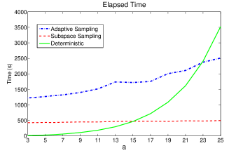
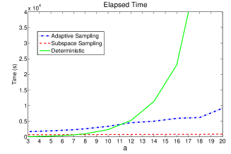
(a) $k=10$, $c=ak$, and $r=ac$.

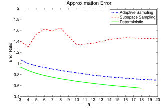
(b) $k=50$, $c=ak$, and $r=ac$.

Figure 1: Results of the CUR algorithms on the Enron data set.

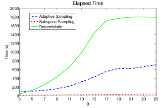
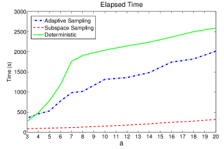
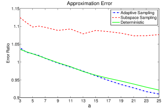
(a) $k=10$, $c=ak$, and $r=ac$.

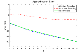
(b) $k=50$, $c=ak$, and $r=ac$.

Figure 2: Results of the CUR algorithms on the Dexter data set.

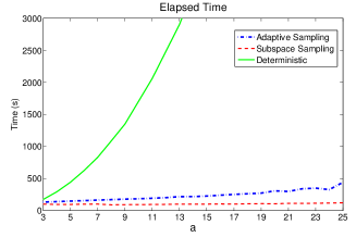
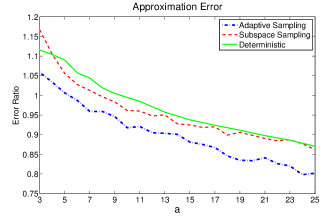
(a) $k=10$, $c=ak$, and $r=ac$.

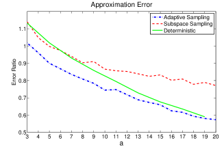
(b) $k=50$, $c=ak$, and $r=ac$.

Figure 3: Results of the CUR algorithms on the Farm Ads data set.

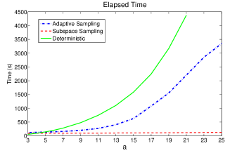
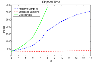
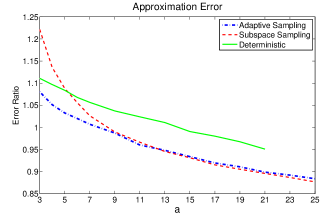
(a) $k=10$, $c=ak$, and $r=ac$.

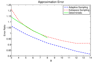
(b) $k=50$, $c=ak$, and $r=ac$.

Figure 4: Results of the CUR algorithms on the Gisette data set.

We conduct experiments on four UCI data sets (Frank and Asuncion, 2010) which are summarized in Table 4. Each data set is represented as a data matrix, upon which we apply the CUR algorithms. According to our analysis, the target rank $k$ should be far less than $m$ and $n$, and the column number $c$ and row number $r$ should be strictly greater than $k$. For each data set and each algorithm, we set $k=10$ or $50$, and $c=ak$, $r=ac$, where $a$ ranges in each set of experiments. We repeat each of the two randomized algorithms $10$ times, and report the minimum error ratio and the total elapsed time of the $10$ rounds. We depict the error ratios and the elapsed time of the three CUR matrix decomposition algorithms in Figures 1, 2, 3, and 4.

We can see from Figures 1, 2, 3, and 4 that our adaptive sampling based CUR algorithm has much lower approximation error than the subspace sampling algorithm in all cases. Our adaptive sampling based algorithm is better than the deterministic SCRA on the Farm Ads data set and the Gisette data set, worse than SCRA on the Enron data set, and comparable to SCRA on the Dexter data set. In addition, the experimental results match our theoretical analysis in Section 4 very well. The empirical results all obey the theoretical relative-error upper bound

$$\frac{\|{\bf A}-{\bf C}{\bf U}{\bf R}\|_{F}}{\|{\bf A}-{\bf A}_{k}\|_{F}}\;\leq\;1+\frac{2k}{c}\big{(}1+o(1)\big{)}\;=\;1+\frac{2}{a}\big{(}1+o(1)\big{)}\textrm{.}$$

As for the running time, the subspace sampling algorithm and our adaptive sampling based algorithm are much more efficient than SCRA, especially when $c$ and $r$ are large. Our adaptive sampling based algorithm is comparable to the subspace sampling algorithm when $c$ and $r$ are small; however, our algorithm becomes less efficient when $c$ and $r$ are large. This is due to the following reasons. First, the computational cost of the subspace sampling algorithm is dominated by the truncated SVD of ${\bf A}$, which is determined by the target rank $k$ and the size and sparsity of the data matrix. However, the cost of our algorithm grows with $c$ and $r$. Thus, our algorithm becomes less efficient when $c$ and $r$ are large. Second, the truncated SVD operation in MATLAB, that is, the ‘$\mathrm{svds}$’ function, gains from sparsity, but our algorithm does not. The four data sets are all very sparse, so the subspace sampling algorithm has advantages. Third, the truncated SVD functions are very well implemented by MATLAB (not in MATLAB language but in Fortran/C). In contrast, our algorithm is implemented in MATLAB language, which is usually less efficient than Fortran/C.

5.2 Comparison among the Nyström Algorithms

In this section we empirically compare our adaptive sampling algorithm (in Theorem 10) with some other sampling algorithms including the subspace sampling of Drineas et al. (2008) and the uniform sampling, both without replacement. We also conduct comparison between the standard Nyström and our modified Nyström, both use the three sampling algorithms to select columns.

We test the algorithms on three data sets which are summarized in Table 5. The experiment setting follows Gittens and Mahoney (2013). For each data set we generate a radial basis function (RBF) kernel matrix ${\bf A}$ which is defined by

$$a_{ij}=\exp\bigg{(}-\frac{\|{\bf x}_{i}-{\bf x}_{j}\|_{2}^{2}}{2\sigma^{2}}\bigg{)},$$

where ${\bf x}_{i}$ and ${\bf x}_{j}$ are data instances and $\sigma$ is a scale parameter. Notice that the RBF kernel is dense in general. We set $\sigma=0.2$ or $1$ in our experiments. For each data set with different settings of $\sigma$, we fix a target rank $k=10$, $20$ or $50$ and vary $c$ in a very large range. We will discuss the choice of $\sigma$ and $k$ in the following two paragraphs. We run each algorithm for $10$ times, and report the the minimum error ratio as well as the total elapsed time of the $10$ repeats. The results are shown in Figures 5, 6, and 7.

Data Set	#Instances	#Attributes	Source
Abalone	$4,177$	$8$	UCI (Frank and Asuncion, 2010)
Wine Quality	$4,898$	$12$	UCI (Cortez et al., 2009)
Letters	$5,000$	$16$	Statlog (Michie et al., 1994)

	${\|{\bf A}-{\bf A}_{k}\|_{F}}/{\|{\bf A}\|_{F}}$			$\frac{m}{k}\mathsf{std}\big{(}\mathbf{\ell}^{[k]}\big{)}$
	$k=10$	$k=20$	$k=50$	$k=10$	$k=20$	$k=50$
Abalone ($\sigma=0.2$)	$0.4689$	$0.3144$	$0.1812$	$0.8194$	$0.6717$	$0.4894$
Abalone ($\sigma=1.0$)	$0.0387$	$0.0122$	$0.0023$	$0.5879$	$0.8415$	$1.3830$
Wine Quality ($\sigma=0.2$)	$0.8463$	$0.7930$	$0.7086$	$1.8703$	$1.6490$	$1.3715$
Wine Quality ($\sigma=1.0$)	$0.0504$	$0.0245$	$0.0084$	$0.3052$	$0.5124$	$0.8067$
Letters ($\sigma=0.2$)	$0.9546$	$0.9324$	$0.8877$	$5.4929$	$3.9346$	$2.6210$
Letters ($\sigma=1.0$)	$0.1254$	$0.0735$	$0.0319$	$0.2481$	$0.2938$	$0.3833$

Table 5: A summary of the data sets for the Nyström approximation. In the second tabular $\mathsf{std}\big{(}\mathbf{\ell}^{[k]}\big{)}$ denotes the standard deviation of the statistical leverage scores of ${\bf A}$ relative to the best rank-$k$ approximation to ${\bf A}$. We use the normalization factor $\frac{m}{k}$ because $\frac{m}{k}\mathsf{mean}\big{(}\mathbf{\ell}^{[k]}\big{)}=1$.

Table 5 provides useful implications on choosing the target rank $k$. In Table 5, $\frac{\|{\bf A}-{\bf A}_{k}\|_{F}}{\|{\bf A}\|_{F}}$ denotes ratio that is not captured by the best rank-$k$ approximation to the RBF kernel, and the parameter $\sigma$ has an influence on the ratio ${\|{\bf A}-{\bf A}_{k}\|_{F}}/{\|{\bf A}\|_{F}}$. When $\sigma$ is large, the RBF kernel can be well approximated by a low-rank matrix, which implies that (i) a small $k$ suffices when $\sigma$ is large, and (ii) $k$ should be set large when $\sigma$ is small. So the settings ($\sigma=1$, $k=10$) and ($\sigma=0.2$, $k=50$) are more reasonable than the rest. Let us take the RBF kernel in the Abalone data set as an example. When $\sigma=1$, the rank-$10$ approximation well captures the kernel, so $k$ can be safely set as small as $10$; when $\sigma=0.2$, the target rank $k$ should be set large, say larger than $50$, otherwise the approximation is rough.

The standard deviation of the leverage scores reflects whether the advanced importance sampling techniques such as the subspace sampling and adaptive sampling are useful. Figures 5, 6, and 7 show that the advantage of the subspace sampling and adaptive sampling over the uniform sampling is significant whenever the standard deviation of the leverage scores is large (see Table 5), and vise versa. Actually, as reflected in Table 5, the parameter $\sigma$ influences the homogeneity/heterogeneity of the leverage scores. Usually, when $\sigma$ is small, the leverage scores become heterogeneous, and the effect of choosing “good” columns is significant.

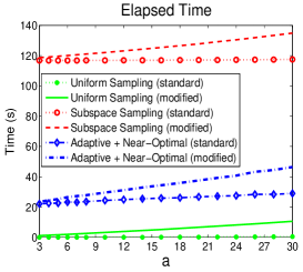
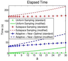
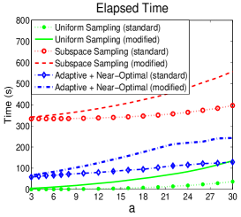
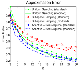
(a) $\sigma=0.2$, $k=10$, and $c=ak$.

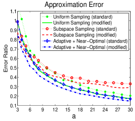
(b) $\sigma=0.2$, $k=20$, and $c=ak$.

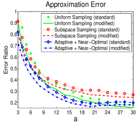
(c) $\sigma=0.2$, $k=50$, and $c=ak$.

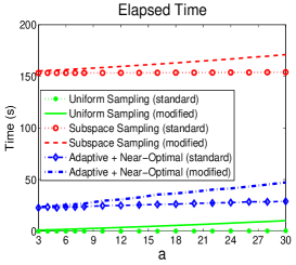
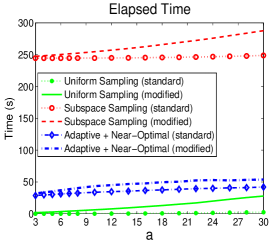
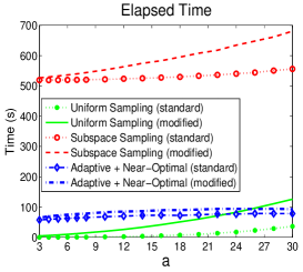
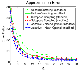
(d) $\sigma=1$, $k=10$, and $c=ak$.

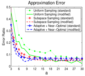
(e) $\sigma=1$, $k=20$, and $c=ak$.

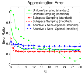
(f) $\sigma=1$, $k=50$, and $c=ak$.

Figure 5: Results of the Nyström algorithms on the RBF kernel in the Abalone data set.

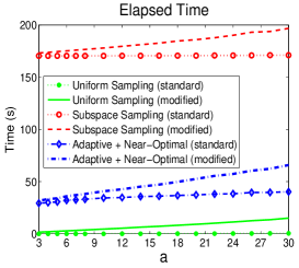
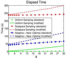
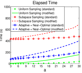
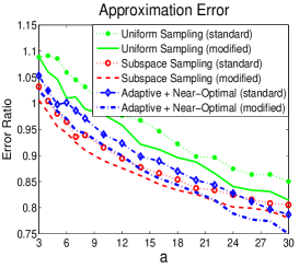
(a) $\sigma=0.2$, $k=10$, and $c=ak$.

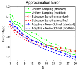
(b) $\sigma=0.2$, $k=20$, and $c=ak$.

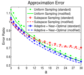
(c) $\sigma=0.2$, $k=50$, and $c=ak$.

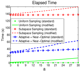
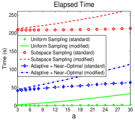
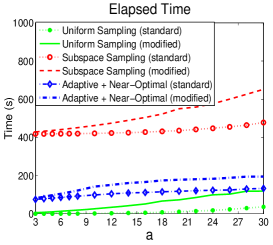
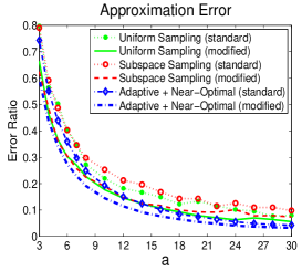
(d) $\sigma=1$, $k=10$, and $c=ak$.

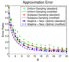
(e) $\sigma=1$, $k=20$, and $c=ak$.

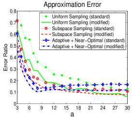
(f) $\sigma=1$, $k=50$, and $c=ak$.

Figure 6: Results of the Nyström algorithms on the RBF kernel in the Wine Quality data set.

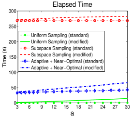
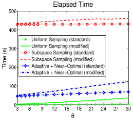
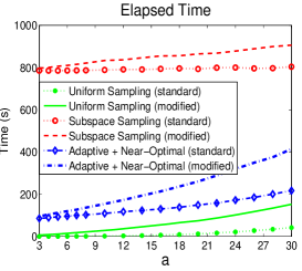
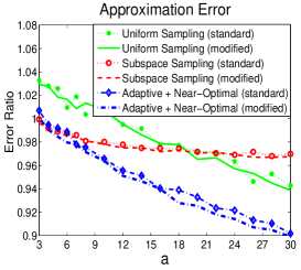
(a) $\sigma=0.2$, $k=10$, and $c=ak$.

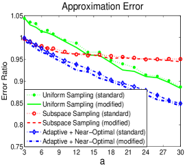
(b) $\sigma=0.2$, $k=20$, and $c=ak$.

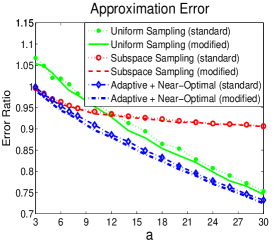
(c) $\sigma=0.2$, $k=50$, and $c=ak$.

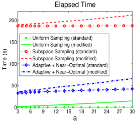
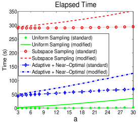
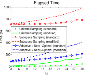
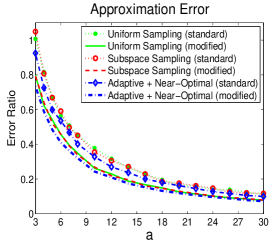
(d) $\sigma=1$, $k=10$, and $c=ak$.

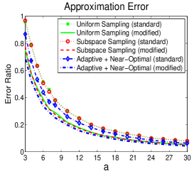
(e) $\sigma=1$, $k=20$, and $c=ak$.

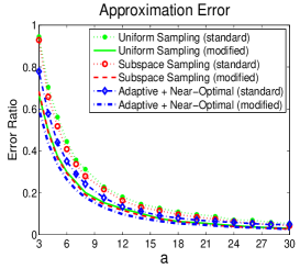
(f) $\sigma=1$, $k=50$, and $c=ak$.

Figure 7: Results of the Nyström algorithms on the RBF kernel in the Letters data set.

The experimental results also show that the subspace sampling and adaptive sampling algorithms significantly outperform the uniform sampling when $c$ is reasonably small, say $c<10k$. This indicates that the subspace sampling and adaptive sampling algorithms are good at choosing “good” columns as basis vectors. The effect is especially evident on the RBF kernel with the scale parameter $\sigma=0.2$, where the leverage scores are heterogeneous. In most cases our adaptive sampling algorithm achieves the lowest approximation error among the three algorithms. The error ratios of our adaptive sampling for the modified Nyström are in accordance with the theoretical bound in Theorem 10; that is,

$$\frac{\|{\bf A}-{\bf C}{\bf U}{\bf C}^{T}\|_{F}}{\|{\bf A}-{\bf A}_{k}\|_{F}}\;\leq\;1+\sqrt{\frac{2k}{c}\big{(}1+o(1)\big{)}}\;=\;1+\sqrt{\frac{2}{a}\big{(}1+o(1)\big{)}}\textrm{.}$$

As for the running time, our adaptive sampling algorithm is more efficient than the subspace sampling algorithm. This is partly because the RBF kernel matrix is dense, and hence the subspace sampling algorithm costs ${\mathcal{O}}(m^{2}k)$ time to compute the truncated SVD.

Furthermore, the experimental results show that using ${\bf U}={\bf C}^{\dagger}{\bf A}({\bf C}^{\dagger})^{T}$ as the intersection matrix (denoted by “modified” in the figures) always leads to much lower error than using ${\bf U}={\bf W}^{\dagger}$ (denoted by “standard”). However, our modified Nyström method costs more time to compute the intersection matrix than the standard Nyström method costs. Recall that the standard Nyström costs ${\mathcal{O}}(c^{3})$ time to compute ${\bf U}={\bf W}^{\dagger}$ and that the modified Nyström costs ${\mathcal{O}}(mc^{2})+T_{\textrm{Multiply}}(m^{2}c)$ time to compute ${\bf U}={\bf C}^{\dagger}{\bf A}({\bf C}^{\dagger})^{T}$. So the users should make a trade-off between time and accuracy and decide whether it is worthwhile to sacrifice extra computational overhead for the improvement in accuracy by using the modified Nyström method.

6 Conclusion

In this paper we have built a novel and more general relative-error bound for the adaptive sampling algorithm. Accordingly, we have devised novel CUR matrix decomposition and Nyström approximation algorithms which demonstrate significant improvement over the classical counterparts. Our relative-error CUR algorithm requires only $c={2k}{\epsilon^{-1}}(1+o(1))$ columns and $r={c}{\epsilon^{-1}}(1{+}\epsilon)$ rows selected from the original matrix. To achieve relative-error bound, the best previous algorithm—the subspace sampling algorithm—requires $c={\mathcal{O}}(k\epsilon^{-2}\log k)$ columns and $r={\mathcal{O}}(c\epsilon^{-2}\log c)$ rows. Our modified Nyström method is different from the conventional Nyström methods in that it uses a different intersection matrix. We have shown that our adaptive sampling algorithm for the modified Nyström achieves relative-error upper bound by sampling only $c={2k}{\epsilon^{-2}}(1{+}o(1))$ columns, which even beats the lower error bounds of the standard Nyström and the ensemble Nyström. Our proposed CUR and Nyström algorithms are scalable because they need only to maintain a small fraction of columns or rows in RAM, and their time complexities are low provided that matrix multiplication can be highly efficiently executed. Finally, the empirical comparison has also demonstrated the effectiveness and efficiency of our algorithms.

Acknowledgments

This work has been supported in part by the Natural Science Foundations of China (No. 61070239) and the Scholarship Award for Excellent Doctoral Student granted by Chinese Ministry of Education.

A The Dual Set Sparsification Algorithm

For the sake of self-contained, we attach the dual set sparsification algorithm and describe some implementation details. The deterministic dual set sparsification algorithm is established by Boutsidis et al. (2011) and severs as an important step in the near-optimal column selection algorithm (described in Lemma 2 and Algorithm 1 in this paper). We show the dual set sparsification algorithm algorithm in Algorithm 3 and its bounds in Lemma 14, and we also analyze the time complexity using our defined notation.

Lemma 14 (Dual Set Spectral-Frobenius Sparsification)

Let ${\mathcal{U}}=\{{\bf x}_{1},\cdots,{\bf x}_{n}\}\subset{\mathbb{R}}^{l}$ $(l<n)$ contain the columns of an arbitrary matrix ${\bf X}\in{\mathbb{R}}^{l\times n}$. Let ${\mathcal{V}}=\{{\bf v}_{1},\cdots,{\bf v}_{n}\}\subset{\mathbb{R}}^{k}$ $(k<n)$ be a decompositions of the identity, that is, $\sum_{i=1}^{n}{\bf v}_{i}{\bf v}_{i}^{T}={\bf I}_{k}$. Given an integer $r$ with $k<r<n$, Algorithm 3 deterministically computes a set of weights $s_{i}\geq 0$ ($i=1,\cdots,n$) at most $r$ of which are non-zero, such that

$$\lambda_{k}\Big{(}\sum_{i=1}^{n}s_{i}{\bf v}_{i}{\bf v}_{i}^{T}\Big{)}\geq\Big{(}1-\sqrt{\frac{k}{r}}\Big{)}^{2}\qquad\mbox{ and }\qquad\mathrm{tr}\Big{(}\sum_{i=1}^{n}s_{i}{\bf x}_{i}{\bf x}_{i}^{T}\Big{)}\leq\|{\bf X}\|_{F}^{2}.$$

The weights $s_{i}$ can be computed deterministically in ${\mathcal{O}}\big{(}rnk^{2}\big{)}+{T_{\mathrm{Multiply}}}\big{(}nl\big{)}$ time.

Here we mention some implementation issues of Algorithm 3 which were not described in detail by Boutsidis et al. (2011). In each iteration the algorithm performs once eigenvalue decomposition: ${\bf A}_{\tau}={\bf W}\mbox{\boldmath$\Lambda$\unboldmath}{\bf W}^{T}$. Here ${\bf A}_{\tau}$ is guaranteed to be SPSD in each iteration. Since

$$\Big{(}{\bf A}_{\tau}-\alpha{\bf I}_{k}\Big{)}^{q}\;=\;{\bf W}\mathsf{Diag}\Big{(}(\lambda_{1}-\alpha)^{q},\cdots,(\lambda_{k}-\alpha)^{q}\Big{)}{\bf W}^{T}\textrm{,}$$

$({\bf A}_{\tau}-(L_{\tau}+1){\bf I}_{k})^{q}$ can be efficiently computed based on the eigenvalue decomposition of ${\bf A}_{\tau}$. With the eigenvalues at hand, $\phi(L,{\bf A}_{\tau})$ can also be computed directly.

The algorithm runs in $r$ iterations. In each iteration, the eigenvalue decomposition of ${\bf A}_{\tau}$ requires ${\mathcal{O}}(k^{3})$, and the $n$ comparisons in Line 6 each requires ${\mathcal{O}}(k^{2})$. Moreover, computing $\|{\bf x}_{i}\|_{2}^{2}$ for each ${\bf x}_{i}$ requires ${T_{\mathrm{Multiply}}}(nl)$. Overall, the running time of Algorithm 3 is at most ${\mathcal{O}}(rk^{3})+{\mathcal{O}}(rnk^{2})+{T_{\mathrm{Multiply}}}(nl)={\mathcal{O}}(rnk^{2})+{T_{\mathrm{Multiply}}}(nl)$.

Algorithm 3 Deterministic Dual Set Spectral-Frobenius Sparsification Algorithm.

1:  Input: ${\mathcal{U}}=\{{\bf x}_{i}\}_{i=1}^{n}\subset{\mathbb{R}}^{l}$, ($l<n$); ${\mathcal{V}}=\{{\bf v}_{i}\}_{i=1}^{n}\subset{\mathbb{R}}^{k}$, with $\sum_{i=1}^{n}{\bf v}_{i}{\bf v}_{i}^{T}={\bf I}_{k}$ ($k<n$); $k<r<n$;

2:  Initialize: ${\bf s}_{0}={\bf 0}$, ${\bf A}_{0}={\bf 0}$;

3:  Compute $\|{\bf x}_{i}\|_{2}^{2}$ for $i=1,\cdots,n$, and then compute $\delta_{U}=\frac{\sum_{i=1}^{n}\|{\bf x}_{i}\|_{2}^{2}}{1-\sqrt{k/r}}$;

4:  for $\tau=0$ to $r-1$ do

5:        Compute the eigenvalue decomposition of ${\bf A}_{\tau}$;

6:        Find any index $j$ in $\{1,\cdots,n\}$ and compute a weight $t>0$ such that

$$\delta_{U}^{-1}\|{\bf x}_{j}\|_{2}^{2}\;\leq\;t^{-1}\;\leq\;\frac{{\bf v}_{j}^{T}\Big{(}{\bf A}_{\tau}-(L_{\tau}+1){\bf I}_{k}\Big{)}^{-2}{\bf v}_{j}}{\phi(L_{\tau}+1,{\bf A}_{\tau})-\phi(L_{\tau},{\bf A}_{\tau})}-{\bf v}_{j}^{T}\Big{(}{\bf A}_{\tau}-(L_{\tau}+1){\bf I}_{k}\Big{)}^{-1}{\bf v}_{j}\textrm{;}$$

where

$$\phi(L,{\bf A})=\sum_{i=1}^{k}\Big{(}\lambda_{i}({\bf A})-L\Big{)}^{-1}\textrm{, }\qquad\qquad\quad L_{\tau}=\tau-\sqrt{rk}\textrm{;}$$

7:        Update the $j$-th component of ${\bf s}_{\tau}$ and ${\bf A}_{\tau}$: $\quad{\bf s}_{\tau+1}[j]={\bf s}_{\tau}[j]+t$, $\quad{\bf A}_{\tau+1}={\bf A}_{\tau}+t{\bf v}_{j}{\bf v}_{j}^{T}$;

8:  end for

9:  return  ${\bf s}=\frac{1-\sqrt{k/r}}{r}{\bf s}_{r}$.

The near-optimal column selection algorithm described in Lemma 2 has three steps: randomized SVD via random projection which costs ${\mathcal{O}}\big{(}mk^{2}\epsilon^{-4/3}\big{)}+{T_{\mathrm{Multiply}}}\big{(}mnk\epsilon^{-2/3}\big{)}$ time, the dual set sparsification algorithm which costs ${\mathcal{O}}\big{(}nk^{3}\epsilon^{-2/3}\big{)}+{T_{\mathrm{Multiply}}}\big{(}mn\big{)}$ time, and the adaptive sampling algorithm which costs ${\mathcal{O}}\big{(}mk^{2}\epsilon^{-4/3}\big{)}+{T_{\mathrm{Multiply}}}\big{(}mnk\epsilon^{-2/3}\big{)}$ time. Therefore, the near-optimal column selection algorithm costs totally ${\mathcal{O}}\big{(}mk^{2}\epsilon^{-4/3}+nk^{3}\epsilon^{-2/3}\big{)}+{T_{\mathrm{Multiply}}}\big{(}mnk\epsilon^{-2/3}\big{)}$ time.

B Proofs of the Adaptive Sampling Bounds

We present the proofs of Theorem 5, Corollary 7, Theorem 8, and Theorem 10 in Appendices B.1, B.2, B.3, and B.4, respectively.

B.1 The Proof of Theorem 5

Theorem 5 can be equivalently expressed in Theorem 15. In order to stick to the column space convention throughout this paper, we prove Theorem 15 instead of Theorem 5.

Theorem 15 (The Adaptive Sampling Algorithm)

Given a matrix ${\bf A}\in{{\mathbb{R}}^{m\times n}}$ and a matrix ${\bf R}\in{\mathbb{R}}^{r\times n}$ such that $\mathrm{rank}({\bf R})=\mathrm{rank}({\bf A}{\bf R}^{\dagger}{\bf R})=\rho$ $(\rho\leq r\leq m)$, let ${\bf C}_{1}\in{\mathbb{R}}^{m\times c_{1}}$ consist of $c_{1}$ columns of ${\bf A}$, and define the residual ${\bf B}={\bf A}-{\bf C}_{1}{\bf C}_{1}^{\dagger}{\bf A}$. For $i=1,\cdots,n$, let

$$p_{i}\;=\;\|{\bf b}_{i}\|_{2}^{2}/\|{\bf B}\|_{F}^{2},$$

where ${\bf b}_{i}$ is the $i$-th column of the matrix ${\bf B}$. Sample further $c_{2}$ columns from ${\bf A}$ in $c_{2}$ i.i.d. trials, where in each trial the $i$-th column is chosen with probability $p_{i}$. Let ${\bf C}_{2}\in{\mathbb{R}}^{m\times c_{2}}$ contain the $c_{2}$ sampled columns and ${\bf C}=[{\bf C}_{1},{\bf C}_{2}]\in{\mathbb{R}}^{m\times(c_{1}+c_{2})}$ contain the columns of both ${\bf C}_{1}$ and ${\bf C}_{2}$, all of which are columns of ${\bf A}$. Then the following inequality holds:

$${\mathbb{E}}\|{\bf A}-{\bf C}{{\bf C}^{{\dagger}}}{\bf A}{\bf R}^{\dagger}{\bf R}\|_{F}^{2}\;\leq\;\|{\bf A}-{\bf A}{\bf R}^{\dagger}{\bf R}\|_{F}^{2}+\frac{\rho}{c_{2}}\|{\bf A}-{\bf C}_{1}{\bf C}_{1}^{\dagger}{\bf A}\|_{F}^{2}.$$

where the expectation is taken w.r.t. ${\bf C}_{2}$.

Proof  With a little abuse of symbols, we use bold uppercase letters to denote random matrices and bold lowercase to denote random vectors, without distinguishing between random matrices/vectors and non-random matrices/vectors.

We denote the $j$-th column of ${\bf V}_{{\bf A}{\bf R}^{\dagger}{\bf R},\rho}\in{\mathbb{R}}^{n\times\rho}$ as ${\bf v}_{j}$, and the $(i,j)$-th entry of ${\bf V}_{{\bf A}{\bf R}^{\dagger}{\bf R},\rho}$ as $v_{ij}$. Define random vectors ${\bf x}_{j,(l)}\in{\mathbb{R}}^{m}$ such that for $j=1,\cdots,n$ and $l=1,\cdots,c_{2}$,

$${\bf x}_{j,(l)}=\frac{v_{ij}}{p_{i}}{\bf b}_{i}=\frac{v_{ij}}{p_{i}}\Big{(}{\bf a}_{i}-{\bf C}_{1}{\bf C}_{1}^{\dagger}{\bf a}_{i}\Big{)}\quad\textrm{with probability }p_{i}\textrm{,}\quad\textrm{for }i=1,\cdots,n\textrm{,}$$

Notice that ${\bf x}_{j,(l)}$ is a linear function of a column of ${\bf A}$ sampled from the above defined distribution. We have that

$${\mathbb{E}}[{\bf x}_{j,(l)}] = \sum_{i=1}^{n}p_{i}\frac{v_{ij}}{p_{i}}{\bf b}_{i}\quad=\quad{\bf B}{\bf v}_{j}\textrm{,}$$

$${\mathbb{E}}\|{\bf x}_{j,(l)}\|_{2}^{2} = \sum_{i=1}^{n}p_{i}\frac{v^{2}_{ij}}{p_{i}^{2}}\|{\bf b}_{i}\|_{2}^{2}\quad=\quad\sum_{i=1}^{n}\frac{v^{2}_{ij}}{\|{\bf b}_{i}\|_{2}^{2}/\|{\bf B}\|_{F}^{2}}\|{\bf b}_{i}\|_{2}^{2}\quad=\quad\|{\bf B}\|_{F}^{2}\textrm{.}$$

Then we let ${\bf x}_{j}=\frac{1}{c_{2}}\sum_{l=1}^{c_{2}}{\bf x}_{j,(l)}$, we have

$${\mathbb{E}}[{\bf x}_{j}] = {\mathbb{E}}[{\bf x}_{j,(l)}]\quad=\quad{\bf B}{\bf v}_{j}\textrm{,}$$

$${\mathbb{E}}\|{\bf x}_{j}-{\bf B}{\bf v}_{j}\|_{2}^{2} = {\mathbb{E}}\Big{\|}{\bf x}_{j}-{\mathbb{E}}[{\bf x}_{j}]\Big{\|}_{2}^{2}=\frac{1}{c_{2}}{\mathbb{E}}\Big{\|}{\bf x}_{j,(l)}-{\mathbb{E}}[{\bf x}_{j,(l)}]\Big{\|}_{2}^{2}=\frac{1}{c_{2}}{\mathbb{E}}\|{\bf x}_{j,(l)}-{\bf B}{\bf v}_{j}\|_{2}^{2}\textrm{.}$$

According to the construction of ${\bf x}_{1},\cdots,{\bf x}_{\rho}$, we define the $c_{2}$ columns of ${\bf A}$ to be ${\bf C}_{2}\in{\mathbb{R}}^{m\times c_{2}}$. Note that all the random vectors ${\bf x}_{1}\cdots,{\bf x}_{\rho}$ lie in the subspace $\mathrm{span}({\bf C}_{1})+\mathrm{span}({\bf C}_{2})$. We define random vectors

$${\bf w}_{j}={\bf C}_{1}{\bf C}_{1}^{\dagger}{\bf A}{\bf R}^{\dagger}{\bf R}{\bf v}_{j}+{\bf x}_{j}={\bf C}_{1}{\bf C}_{1}^{\dagger}{\bf A}{\bf v}_{j}+{\bf x}_{j}\textrm{,}\qquad\textrm{for }j=1,\cdots,\rho\textrm{,}$$

where the second equality follows from Lemma 16; that is, ${\bf A}{\bf R}^{\dagger}{\bf R}{\bf v}_{j}={\bf A}{\bf v}_{j}$ if ${\bf v}_{j}$ is one of the top $\rho$ right singular vectors of ${\bf A}{\bf R}^{\dagger}{\bf R}$. Then we have that any set of random vectors $\{{\bf w}_{1},\cdots,{\bf w}_{\rho}\}$ lies in $\mathrm{span}({\bf C})=\mathrm{span}({\bf C}_{1})+\mathrm{span}({\bf C}_{2})$. Let ${\bf W}=[{\bf w}_{1},\cdots,{\bf w}_{\rho}]$ be a random matrix, we have that $\mathrm{span}({\bf W})\subset\mathrm{span}({\bf C})$. The expectation of ${\bf w}_{j}$ is

$${\mathbb{E}}[{\bf w}_{j}]={\bf C}_{1}{\bf C}_{1}^{\dagger}{\bf A}{\bf v}_{j}+{\mathbb{E}}[{\bf x}_{j}]={\bf C}_{1}{\bf C}_{1}^{\dagger}{\bf A}{\bf v}_{j}+{\bf B}{\bf v}_{j}={\bf A}{\bf v}_{j}\textrm{,}$$

therefore we have that

$${\bf w}_{j}-{\bf A}{\bf v}_{j}={\bf x}_{j}-{\bf B}{\bf v}_{j}\textrm{.}$$

The expectation of $\|{\bf w}_{j}-{\bf A}{\bf v}_{j}\|_{2}^{2}$ is

$${\mathbb{E}}\|{\bf w}_{j}-{\bf A}{\bf v}_{j}\|_{2}^{2} = {\mathbb{E}}\|{\bf x}_{j}-{\bf B}{\bf v}_{j}\|_{2}^{2}\quad=\quad\frac{1}{c_{2}}{\mathbb{E}}\|{\bf x}_{j,(l)}-{\bf B}{\bf v}_{j}\|_{2}^{2}$$ (5)

$$= \frac{1}{c_{2}}{\mathbb{E}}\|{\bf x}_{j,(l)}\|_{2}^{2}-\frac{2}{c_{2}}({\bf B}{\bf v}_{j})^{T}{\mathbb{E}}[{\bf x}_{j,(l)}]+\frac{1}{c_{2}}\|{\bf B}{\bf v}_{j}\|_{2}^{2}$$

$$= \frac{1}{c_{2}}{\mathbb{E}}\|{\bf x}_{j,(l)}\|_{2}^{2}-\frac{1}{c_{2}}\|{\bf B}{\bf v}_{j}\|_{2}^{2}\quad=\quad\frac{1}{c_{2}}\|{\bf B}\|_{F}^{2}-\frac{1}{c_{2}}\|{\bf B}{\bf v}_{j}\|_{2}^{2}$$

$$\leq \frac{1}{c_{2}}\|{\bf B}\|_{F}^{2}\textrm{.}$$

To complete the proof, we denote

$${\bf F}=(\sum_{q=1}^{\rho}\sigma_{q}^{-1}{\bf w}_{q}{\bf u}_{q}^{T}){\bf A}{\bf R}^{\dagger}{\bf R}\textrm{,}$$

where $\sigma_{q}$ is the $q$-th largest singular value of ${\bf A}{\bf R}^{\dagger}{\bf R}$ and ${\bf u}_{q}$ is the corresponding left singular vector of ${\bf A}{\bf R}^{\dagger}{\bf R}$. The column space of ${\bf F}$ is contained in $\mathrm{span}({\bf W})$ ($\subset\mathrm{span}({\bf C})$), and thus

$$\|{\bf A}{\bf R}^{\dagger}{\bf R}-{\bf C}{\bf C}^{\dagger}{\bf A}{\bf R}^{\dagger}{\bf R}\|_{F}^{2}\leq\|{\bf A}{\bf R}^{\dagger}{\bf R}-{\bf W}{\bf W}^{\dagger}{\bf A}{\bf R}^{\dagger}{\bf R}\|_{F}^{2}\leq\|{\bf A}{\bf R}^{\dagger}{\bf R}-{\bf F}\|_{F}^{2}\textrm{.}$$

We use ${\bf F}$ to bound the error $\|{\bf A}{\bf R}^{\dagger}{\bf R}-{\bf C}{\bf C}^{\dagger}{\bf A}{\bf R}^{\dagger}{\bf R}\|_{F}^{2}$. That is,

$${\mathbb{E}}\|{\bf A}-{\bf C}{\bf C}^{\dagger}{\bf A}{\bf R}^{\dagger}{\bf R}\|_{F}^{2} = {\mathbb{E}}\|{\bf A}-{\bf A}{\bf R}^{\dagger}{\bf R}+{\bf A}{\bf R}^{\dagger}{\bf R}-{\bf C}{\bf C}^{\dagger}{\bf A}{\bf R}^{\dagger}{\bf R}\|_{F}^{2}$$

$$= {\mathbb{E}}\Big{[}\|{\bf A}-{\bf A}{\bf R}^{\dagger}{\bf R}\|_{F}^{2}+\|{\bf A}{\bf R}^{\dagger}{\bf R}-{\bf C}{\bf C}^{\dagger}{\bf A}{\bf R}^{\dagger}{\bf R}\|_{F}^{2}\Big{]}$$

$$\leq \|{\bf A}-{\bf A}{\bf R}^{\dagger}{\bf R}\|_{F}^{2}+{\mathbb{E}}\|{\bf A}{\bf R}^{\dagger}{\bf R}-{\bf F}\|_{F}^{2}\textrm{,}$$

where (B.1) is due to that ${\bf A}({\bf I}-{\bf R}^{\dagger}{\bf R})$ is orthogonal to $({\bf I}-{\bf C}{\bf C}^{\dagger}){\bf A}{\bf R}^{\dagger}{\bf R}$. Since ${\bf A}{\bf R}^{\dagger}{\bf R}$ and ${\bf F}$ both lie on the space spanned by the right singular vectors of ${{\bf A}{\bf R}^{\dagger}{\bf R}}$ (i.e., $\{{\bf v}_{j}\}_{j=1}^{\rho}$), we decompose ${\bf A}{\bf R}^{\dagger}{\bf R}-{\bf F}$ along $\{{\bf v}_{j}\}_{j=1}^{\rho}$, obtaining that

$${\mathbb{E}}\|{\bf A}-{\bf C}{\bf C}^{\dagger}{\bf A}{\bf R}^{\dagger}{\bf R}\|_{F}^{2} \leq \|{\bf A}-{\bf A}{\bf R}^{\dagger}{\bf R}\|_{F}^{2}+{\mathbb{E}}\|{\bf A}{\bf R}^{\dagger}{\bf R}-{\bf F}\|_{F}^{2}\textrm{,}$$ (7)

$$= \|{\bf A}-{\bf A}{\bf R}^{\dagger}{\bf R}\|_{F}^{2}+\sum_{j=1}^{\rho}{\mathbb{E}}\Big{\|}({\bf A}{\bf R}^{\dagger}{\bf R}-{\bf F}){\bf v}_{j}\Big{\|}_{2}^{2}$$

$$= \|{\bf A}-{\bf A}{\bf R}^{\dagger}{\bf R}\|_{F}^{2}+\sum_{j=1}^{\rho}{\mathbb{E}}\Big{\|}{\bf A}{\bf R}^{\dagger}{\bf R}{\bf v}_{j}-(\sum_{q=1}^{\rho}\sigma_{q}^{-1}{\bf w}_{q}{\bf u}_{q}^{T})\sigma_{j}{\bf u}_{j}\Big{\|}_{2}^{2}$$

$$= \|{\bf A}-{\bf A}{\bf R}^{\dagger}{\bf R}\|_{F}^{2}+\sum_{j=1}^{\rho}{\mathbb{E}}\Big{\|}{\bf A}{\bf R}^{\dagger}{\bf R}{\bf v}_{j}-{\bf w}_{j}\Big{\|}_{2}^{2}$$

$$= \|{\bf A}-{\bf A}{\bf R}^{\dagger}{\bf R}\|_{F}^{2}+\sum_{j=1}^{\rho}{\mathbb{E}}\|{\bf A}{\bf v}_{j}-{\bf w}_{j}\|_{2}^{2}$$

$$\leq \|{\bf A}-{\bf A}{\bf R}^{\dagger}{\bf R}\|_{F}^{2}+\frac{\rho}{c_{2}}\|{\bf B}\|_{F}^{2}\textrm{,}$$ (8)

where (7) follows from Lemma 16 and (8) follows from (5).  

Lemma 16

We are given a matrix ${\bf A}\in{{\mathbb{R}}^{m\times n}}$ and a matrix ${\bf R}\in{\mathbb{R}}^{r\times n}$ such that $\mathrm{rank}({\bf A}{\bf R}^{\dagger}{\bf R})=\mathrm{rank}({\bf R})=\rho$ $(\rho\leq r\leq m)$. Letting ${\bf v}_{j}\in{\mathbb{R}}^{n}$ be the $j$-th top right singular vector of ${\bf A}{\bf R}^{\dagger}{\bf R}$, we have that

$${\bf A}{\bf R}^{\dagger}{\bf R}{\bf v}_{j}\;=\;{\bf A}{\bf v}_{j}\textrm{,}\qquad\textrm{for }j=1,\cdots,\rho\textrm{.}$$

Proof  First let ${\bf V}_{{\bf R},\rho}\in{\mathbb{R}}^{n\times\rho}$ contain the top $\rho$ right singular vectors of ${\bf R}$. Then the projection of ${\bf A}$ onto the row space of ${\bf R}$ is ${\bf A}{\bf R}^{\dagger}{\bf R}={\bf A}{\bf V}_{{\bf R},\rho}{\bf V}_{{\bf R},\rho}^{T}$. Let the thin SVD of ${\bf A}{\bf V}_{{\bf R},\rho}\in{\mathbb{R}}^{m\times\rho}$ be $\tilde{{\bf U}}\tilde{\mbox{\boldmath$\Sigma$\unboldmath}}\tilde{{\bf V}}^{T}$, where $\tilde{{\bf V}}\in{\mathbb{R}}^{\rho\times\rho}$. Then the compact SVD of ${\bf A}{\bf R}^{\dagger}{\bf R}$ is

$${\bf A}{\bf R}^{\dagger}{\bf R}\;=\;{\bf A}{\bf V}_{{\bf R},\rho}{\bf V}_{{\bf R},\rho}^{T}\;=\;\tilde{{\bf U}}\tilde{\mbox{\boldmath$\Sigma$\unboldmath}}\tilde{{\bf V}}^{T}{\bf V}_{{\bf R},\rho}^{T}\textrm{.}$$

According to the definition, ${\bf v}_{j}$ is the $j$-th column of $({\bf V}_{{\bf R},\rho}\tilde{{\bf V}})\in{\mathbb{R}}^{n\times\rho}$. Thus ${\bf v}_{j}$ lies on the column space of ${\bf V}_{{\bf R},\rho}$, and ${\bf v}_{j}$ is orthogonal to ${\bf V}_{{\bf R},\rho\perp}$. Finally, since ${\bf A}-{\bf A}{\bf R}^{\dagger}{\bf R}={\bf A}{\bf V}_{{\bf R},\rho\perp}{\bf V}_{{\bf R},\rho\perp}^{T}$, we have that ${\bf v}_{j}$ is orthogonal to ${\bf A}-{\bf A}{\bf R}^{\dagger}{\bf R}$, that is, $({\bf A}-{\bf A}{\bf R}^{\dagger}{\bf R}){\bf v}_{j}={\bf 0}$, which directly proves the lemma.  

B.2 The Proof of Corollary 7

Since ${\bf C}$ is constructed by columns of ${\bf A}$ and the column space of ${\bf C}$ is contained in the column space of ${\bf A}$, we have $\mathrm{rank}({\bf C}{\bf C}^{\dagger}{\bf A})=\mathrm{rank}({\bf C})=\rho\leq c$. Consequently, the assumptions of Theorem 5 are satisfied. The assumptions in turn imply

$$\|{\bf A}-{\bf C}{\bf C}^{\dagger}{\bf A}\|_{F} \leq (1+\epsilon)\|{\bf A}-{\bf A}_{k}\|_{F}\textrm{,}$$

$$\|{\bf A}-{\bf A}{\bf R}_{1}^{\dagger}{\bf R}_{1}\|_{F} \leq (1+\epsilon)\|{\bf A}-{\bf A}_{k}\|_{F}\textrm{,}$$

and $c/r_{2}=\epsilon$. It then follows from Theorem 5 that

$${\mathbb{E}}_{\bf R}\big{\|}{\bf A}-{\bf C}{{\bf C}^{{\dagger}}}{\bf A}{\bf R}^{\dagger}{\bf R}\big{\|}_{F}^{2} = {\mathbb{E}}_{{\bf R}_{1}}\Big{[}{\mathbb{E}}_{{\bf R}_{2}}\Big{[}\|{\bf A}-{\bf C}{{\bf C}^{{\dagger}}}{\bf A}{\bf R}^{\dagger}{\bf R}\|_{F}^{2}\Big{|}{\bf R}_{1}\Big{]}\Big{]}$$

$$\leq {\mathbb{E}}_{{\bf R}_{1}}\Big{[}\|{\bf A}-{\bf C}{{\bf C}^{{\dagger}}}{\bf A}\|_{F}^{2}+\frac{\rho}{r_{2}}\|{\bf A}-{\bf A}{\bf R}_{1}^{\dagger}{\bf R}_{1}\|_{F}^{2}\Big{]}$$

$$\leq \|{\bf A}-{\bf C}{{\bf C}^{{\dagger}}}{\bf A}\|_{F}^{2}+\frac{c}{r_{2}}(1+\epsilon)\|{\bf A}-{\bf A}_{k}\|_{F}^{2}$$

$$= \|{\bf A}-{\bf C}{{\bf C}^{{\dagger}}}{\bf A}\|_{F}^{2}+\epsilon(1+\epsilon)\|{\bf A}-{\bf A}_{k}\|_{F}^{2}\textrm{.}$$

Furthermore, we have that

$$\Big{[}{\mathbb{E}}\|{\bf A}-{\bf C}{\bf U}{\bf R}\|_{F}\Big{]}^{2} \leq {\mathbb{E}}\|{\bf A}-{\bf C}{\bf U}{\bf R}\|_{F}^{2}\quad=\quad{\mathbb{E}}_{{\bf C},{\bf R}}\|{\bf A}-{\bf C}{{\bf C}^{{\dagger}}}{\bf A}{\bf R}^{\dagger}{\bf R}\|_{F}^{2}$$

$$= {\mathbb{E}}_{{\bf C}}\Big{[}{\mathbb{E}}_{{\bf R}}\Big{[}\|{\bf A}-{\bf C}{{\bf C}^{{\dagger}}}{\bf A}{\bf R}^{\dagger}{\bf R}\|_{F}^{2}\Big{|}{\bf C}\Big{]}\Big{]}$$

$$\leq {\mathbb{E}}_{{\bf C}}\Big{[}\|{\bf A}-{\bf C}{{\bf C}^{{\dagger}}}{\bf A}\|_{F}^{2}+\epsilon(1+\epsilon)\|{\bf A}-{\bf A}_{k}\|_{F}^{2}\Big{]}$$

$$\leq (1+\epsilon)^{2}\|{\bf A}-{\bf A}_{k}\|_{k}^{2}\textrm{,}$$

which yields the error bound for CUR matrix decomposition.

When the matrix ${\bf A}$ is symmetric, the matrix ${\bf C}_{1}^{T}$ consists of the rows ${\bf A}$, and thus we can use Theorem 15 (which is identical to Theorem 5) to prove the error bound for the Nyström approximation. By replacing ${\bf R}$ in Theorem 15 by ${\bf C}_{1}^{T}$, we have that

$${\mathbb{E}}\big{\|}{\bf A}-{\bf C}{\bf C}^{\dagger}{\bf A}{({\bf C}_{1}^{\dagger})}^{T}{{\bf C}_{1}^{T}}\big{\|}_{F}^{2} \leq \big{\|}{\bf A}-{\bf A}{({\bf C}_{1}^{\dagger})}^{T}{{\bf C}_{1}^{T}}\big{\|}_{F}^{2}+\frac{c_{1}}{c_{2}}\big{\|}{\bf A}-{\bf C}_{1}{\bf C}_{1}^{\dagger}{\bf A}\big{\|}_{F}^{2}$$

$$= \Big{(}1+\frac{c_{1}}{c_{2}}\Big{)}\big{\|}{\bf A}-{\bf C}_{1}{\bf C}_{1}^{\dagger}{\bf A}\big{\|}_{F}^{2}\textrm{,}$$

where the expectation is taken w.r.t. ${\bf C}_{2}$. Together with the inequality

$$\big{\|}{\bf A}-{\bf C}{\bf C}^{\dagger}{\bf A}{({\bf C}^{\dagger})}^{T}{{\bf C}^{T}}\big{\|}_{F}^{2}\;\leq\;\big{\|}{\bf A}-{\bf C}{\bf C}^{\dagger}{\bf A}{({\bf C}_{1}^{\dagger})}^{T}{{\bf C}_{1}^{T}}\big{\|}_{F}^{2}$$

given by Lemma 17, we have that

$${\mathbb{E}}_{{\bf C}_{1},{\bf C}_{2}}\big{\|}{\bf A}-{\bf C}{\bf C}^{\dagger}{\bf A}{({\bf C}^{\dagger})}^{T}{{\bf C}^{T}}\big{\|}_{F}^{2} \leq {\mathbb{E}}_{{\bf C}_{1},{\bf C}_{2}}\big{\|}{\bf A}-{\bf C}{\bf C}^{\dagger}{\bf A}{({\bf C}_{1}^{\dagger})}^{T}{{\bf C}_{1}^{T}}\big{\|}_{F}^{2}$$

$$= \Big{(}1+\frac{c_{1}}{c_{2}}\Big{)}{\mathbb{E}}_{{\bf C}_{1}}\big{\|}{\bf A}-{\bf C}_{1}{\bf C}_{1}^{\dagger}{\bf A}\big{\|}_{F}^{2}$$

$$= (1{+}\epsilon)^{2}\big{\|}{\bf A}{-}{\bf A}_{k}\big{\|}_{F}^{2}\textrm{.}$$

Hence ${\mathbb{E}}\big{\|}{\bf A}{-}{\bf C}{\bf C}^{\dagger}{\bf A}{({\bf C}^{\dagger})}^{T}{{\bf C}^{T}}\big{\|}_{F}\leq\Big{[}{\mathbb{E}}\big{\|}{\bf A}{-}{\bf C}{\bf C}^{\dagger}{\bf A}{({\bf C}^{\dagger})}^{T}{{\bf C}^{T}}\big{\|}_{F}^{2}\Big{]}^{-\frac{1}{2}}\leq(1{+}\epsilon)\big{\|}{\bf A}{-}{\bf A}_{k}\big{\|}_{F}$.

Lemma 17

Given an $m{\times}m$ matrix ${\bf A}$ and an $m{\times}c$ matrix ${\bf C}=[{\bf C}_{1},{\bf C}_{2}]$, the following inequality holds:

$$\big{\|}{\bf A}-{\bf C}{\bf C}^{\dagger}{\bf A}{({\bf C}^{\dagger})}^{T}{{\bf C}^{T}}\big{\|}_{F}^{2}\;\leq\;\big{\|}{\bf A}-{\bf C}{\bf C}^{\dagger}{\bf A}{({\bf C}_{1}^{\dagger})}^{T}{{\bf C}_{1}^{T}}\big{\|}_{F}^{2}\textrm{.}$$

Proof  Let ${\mathcal{P}}_{\bf C}{\bf A}={\bf C}{\bf C}^{\dagger}{\bf A}$ denote the projection of ${\bf A}$ onto the column space of ${\bf C}$, and $\bar{{\mathcal{P}}}_{\bf C}={\bf I}_{m}-{\bf C}{\bf C}^{\dagger}$ denote the projector onto the space orthogonal to the column space of ${\bf C}$. It has been shown by Halko et al. (2011) that, for any matrix ${\bf A}$, if $\mathrm{span}({\bf M})\subset\mathrm{span}({\bf N})$, then the following inequalities hold:

$$\|{\mathcal{P}}_{\bf M}{\bf A}\|_{\xi}\leq\|{\mathcal{P}}_{\bf N}{\bf A}\|_{\xi}\quad\textrm{ and }\quad\|\bar{{\mathcal{P}}}_{\bf M}{\bf A}\|_{\xi}\geq\|\bar{{\mathcal{P}}}_{\bf N}{\bf A}\|_{\xi}\textrm{.}$$

Accordingly, ${\bf A}{\mathcal{P}}^{T}_{{\bf R}^{T}}={\bf A}{\bf R}^{\dagger}{\bf R}$ is the projection of ${\bf A}$ onto the row space of ${\bf R}\in{\mathbb{R}}^{r\times n}$. We further have that

$$\|{\bf A}-{\mathcal{P}}_{\bf C}{\bf A}{\mathcal{P}}^{T}_{\bf C}\|_{F}^{2} = \|{\bf A}-{\mathcal{P}}_{\bf C}{\bf A}+{\mathcal{P}}_{\bf C}{\bf A}-{\mathcal{P}}_{\bf C}{\bf A}{\mathcal{P}}^{T}_{\bf C}\|_{F}^{2}$$

$$= \|\bar{{\mathcal{P}}}_{\bf C}{\bf A}+{\mathcal{P}}_{\bf C}{\bf A}\bar{{\mathcal{P}}}^{T}_{\bf C}\|_{F}^{2}\;=\;\|\bar{{\mathcal{P}}}_{\bf C}{\bf A}\|_{F}^{2}+\|{\mathcal{P}}_{\bf C}{\bf A}\bar{{\mathcal{P}}}^{T}_{\bf C}\|_{F}^{2}$$

and

$$\|{\bf A}-{\mathcal{P}}_{\bf C}{\bf A}{\mathcal{P}}^{T}_{{\bf C}_{1}}\|_{F}^{2} = \|{\bf A}-{\mathcal{P}}_{\bf C}{\bf A}+{\mathcal{P}}_{\bf C}{\bf A}-{\mathcal{P}}_{\bf C}{\bf A}{\mathcal{P}}^{T}_{{\bf C}_{1}}\|_{F}^{2}$$

$$= \|\bar{{\mathcal{P}}}_{\bf C}{\bf A}+{\mathcal{P}}_{\bf C}{\bf A}\bar{{\mathcal{P}}}^{T}_{{\bf C}_{1}}\|_{F}^{2}\;=\;\|\bar{{\mathcal{P}}}_{\bf C}{\bf A}\|_{F}^{2}+\|{\mathcal{P}}_{\bf C}{\bf A}\bar{{\mathcal{P}}}^{T}_{{\bf C}_{1}}\|_{F}^{2}\textrm{,}$$

where the last equalities follow from ${\mathcal{P}}_{\bf C}\perp\bar{{\mathcal{P}}}_{\bf C}$. Since $\mathrm{span}({\bf C}_{1})\subset\mathrm{span}({\bf C})$, we have $\|{\mathcal{P}}_{\bf C}{\bf A}\bar{{\mathcal{P}}}^{T}_{{\bf C}_{1}}\|_{F}^{2}\geq\|{\mathcal{P}}_{\bf C}{\bf A}\bar{{\mathcal{P}}}^{T}_{{\bf C}}\|_{F}^{2}$, which proves the lemma.  

B.3 The Proof of Theorem 8

The error bound follows directly from Lemma 2 and Corollary 7. The near-optimal column selection algorithm costs ${\mathcal{O}}\big{(}mk^{2}\epsilon^{-4/3}+nk^{3}\epsilon^{-2/3}\big{)}+{T_{\mathrm{Multiply}}}\big{(}mnk\epsilon^{-2/3}\big{)}$ time to construct ${\bf C}$ and ${\mathcal{O}}\big{(}nk^{2}\epsilon^{-4/3}+mk^{3}\epsilon^{-2/3}\big{)}+{T_{\mathrm{Multiply}}}\big{(}mnk\epsilon^{-2/3}\big{)}$ time to construct ${\bf R}_{1}$. Then the adaptive sampling algorithm costs ${\mathcal{O}}\big{(}nk^{2}\epsilon^{-2}\big{)}+{T_{\mathrm{Multiply}}}\big{(}mnk\epsilon^{-1}\big{)}$ time to construct ${\bf R}_{2}$. Computing the Moore-Penrose inverses of ${\bf C}$ and ${\bf R}$ costs ${\mathcal{O}}(mc^{2})+{\mathcal{O}}(nr^{2})={\mathcal{O}}\big{(}mk^{2}\epsilon^{-2}+nk^{2}\epsilon^{-4}\big{)}$ time. The multiplication of ${\bf C}^{\dagger}{\bf A}{\bf R}^{\dagger}$ costs ${T_{\mathrm{Multiply}}}(mnc)={T_{\mathrm{Multiply}}}(mnk\epsilon^{-1})$ time. So the total time complexity is ${\mathcal{O}}\big{(}(m+n)k^{3}\epsilon^{-2/3}+mk^{2}\epsilon^{-2}+nk^{2}\epsilon^{-4}\big{)}+{T_{\mathrm{Multiply}}}\big{(}mnk\epsilon^{-1}\big{)}$.

B.4 The Proof of Theorem 10

The error bound follows immediately from Lemma 2 and Corollary 7. The near-optimal column selection algorithm costs ${\mathcal{O}}\big{(}mk^{2}\epsilon^{-4/3}+mk^{3}\epsilon^{-2/3}\big{)}+{T_{\mathrm{Multiply}}}\big{(}m^{2}k\epsilon^{-2/3}\big{)}$ time to select $c_{1}={\mathcal{O}}(k\epsilon^{-1})$ columns of ${\bf A}$ construct ${\bf C}_{1}$. Then the adaptive sampling algorithm costs ${\mathcal{O}}\big{(}mk^{2}\epsilon^{-2}\big{)}+{T_{\mathrm{Multiply}}}\big{(}m^{2}k\epsilon^{-1}\big{)}$ time to select $c_{2}={\mathcal{O}}(k\epsilon^{-2})$ columns construct ${\bf C}_{2}$. Finally it costs ${\mathcal{O}}(mc^{2})+{T_{\mathrm{Multiply}}}(m^{2}c)={\mathcal{O}}(mk^{2}\epsilon^{-4})+{T_{\mathrm{Multiply}}}\big{(}m^{2}k\epsilon^{-2}\big{)}$ time to construct the intersection matrix ${\bf U}={\bf C}^{\dagger}{\bf A}({\bf C}^{\dagger})^{T}$. So the total time complexity is ${\mathcal{O}}\big{(}mk^{2}\epsilon^{-4}+mk^{3}\epsilon^{-2/3}\big{)}+{T_{\mathrm{Multiply}}}\big{(}m^{2}k\epsilon^{-2}\big{)}$.

C Proofs of the Lower Error Bounds

In Appendix C.1 we construct two adversarial cases which will be used throughout this appendix. In Appendix C.2 we prove the lower bounds of the standard Nyström method. In Appendix C.3 we prove the lower bounds of the ensemble Nyström method. Theorems 20, 21, 22, 24, and 25 are used for proving Theorem 12.

C.1 Construction of the Adversarial Cases

We now consider the construction of adversarial cases for the spectral norm bounds and the Frobenius norm and nuclear norm bounds, respectively.

C.1.1 The Adversarial Case for the Spectral Norm Bound

We construct an $m{\times}m$ positive definite matrix ${\bf B}$ as follows:

$${\bf B}=(1-\alpha){\bf I}_{m}+\alpha{\bf 1}_{m}{\bf 1}_{m}^{T}=\left[\begin{array}[]{cccc}1&\alpha&\cdots&\alpha\\ \alpha&1&\cdots&\alpha\\ \vdots&\vdots&\ddots&\vdots\\ \alpha&\alpha&\cdots&1\\ \end{array}\right]=\left[\begin{array}[]{cc}{\bf W}&{\bf B}_{21}^{T}\\ {\bf B}_{21}&{\bf B}_{22}\\ \end{array}\right]\textrm{,}$$ (9)

where $\alpha\in[0,1)$. It is easy to verify ${\bf x}^{T}{\bf B}{\bf x}>0$ for any nonzero ${\bf x}\in{\mathbb{R}}^{m}$. We show some properties of ${\bf B}$ in Lemma 18.

Lemma 18

Let ${\bf B}_{k}$ be the best rank-$k$ approximation to the matrix ${\bf B}$ defined in (9). Then we have that

$$\|{\bf B}\|_{F}\;=\;\sqrt{m^{2}\alpha^{2}+m(1-\alpha^{2})}\textrm{, } \quad\|{\bf B}-{\bf B}_{k}\|_{F}\;=\;\sqrt{m-k}\,(1-\alpha)\textrm{, }$$

$$\|{\bf B}\|_{2}\;=\;1+m\alpha-\alpha\textrm{ , } \quad\|{\bf B}-{\bf B}_{k}\|_{2}\;=\;1-\alpha\textrm{,}$$

$$\|{\bf B}\|_{*}\;=\;m\textrm{,} \quad\|{\bf B}-{\bf B}_{k}\|_{*}\;=\;(m-k)(1-\alpha)\textrm{, }$$

where $1\leq k\leq m-1$.

Proof  The squared Frobenius norm of ${\bf B}$ is

$$\|{\bf B}\|_{F}^{2}\;=\;\sum_{i,j}b_{ij}^{2}\;=\;m+(m^{2}-m)\alpha^{2}.$$

Then we study the singular values of ${\bf B}$. Since ${\bf B}$ is SPSD, here we do not distinguish between its singular values and eigenvalues.

The spectral norm, that is, the largest singular value, of ${\bf B}$ is

$$\|{\bf B}\|_{2}\;=\;\sigma_{1}\;=\;\lambda_{1}\;=\;\max_{\|{\bf x}\|_{2}\leq 1}{\bf x}^{T}{\bf B}{\bf x}\;=\;\max_{\|{\bf x}\|_{2}\leq 1}(1-\alpha)\|{\bf x}\|_{2}^{2}+\alpha({\bf 1}_{m}^{T}{\bf x})^{2}\;=\;1-\alpha+m\alpha\textrm{,}$$

where the maximum is attained when ${\bf x}=\frac{1}{\sqrt{m}}{\bf 1}_{m}$. Thus ${\bf u}_{1}=\frac{1}{\sqrt{m}}{\bf 1}_{m}$ is the top singular vector of ${\bf B}$. Then the projection of ${\bf B}$ onto the subspace orthogonal to ${\bf u}_{1}$ is

$${\bf B}_{1\perp}\triangleq{\bf B}-{\bf B}_{1}\;=\;{\bf B}-\sigma_{1}{\bf u}_{1}{\bf u}_{1}^{T}\;=\;\frac{1-\alpha}{m}(m{\bf I}_{m}-{\bf 1}_{m}{\bf 1}_{m}^{T}).$$

Then for all $j>1$, the $j$-th top eigenvalue $\sigma_{j}$ and eigenvector ${\bf u}_{j}$, that is, the singular value and singular vector, of ${\bf B}$ satisfy

$$\sigma_{j}{\bf u}_{j}\;=\;{\bf B}{\bf u}_{j}\;=\;{\bf B}_{1\perp}{\bf u}_{j}\;=\;\frac{1-\alpha}{m}\big{(}m{\bf u}_{j}-({\bf 1}_{m}^{T}{\bf u}_{j}){\bf 1}_{m}\big{)}\;=\;\frac{1-\alpha}{m}(m{\bf u}_{j}-{\bf 0}),$$

where the last equality follows from ${\bf u}_{j}\perp{\bf u}_{1}$, that is, ${\bf 1}_{m}^{T}{\bf u}_{j}=0$. Thus $\sigma_{j}=1-\alpha$, and

$$\|{\bf B}-{\bf B}_{k}\|_{2}\;=\;\sigma_{k+1}\;=\;1-\alpha$$

for all $1\leq k<m$. Finally we have that

$$\|{\bf B}-{\bf B}_{k}\|_{F}^{2} = \|{\bf B}\|_{F}^{2}-\sum_{i=1}^{k}\sigma_{i}^{2}\;=\;(m-k)(1-\alpha)^{2}\textrm{,}$$

$$\|{\bf B}-{\bf B}_{k}\|_{*} = (m-k)\sigma_{2}\;=\;(m-k)(1-\alpha)\textrm{,}$$

$$\|{\bf B}\|_{*} = \sum_{i=1}^{m}\sigma_{i}\;=\;(1+m\alpha-\alpha)+(m-1)(1-\alpha)\;=\;m\textrm{,}$$

which complete our proofs.  

C.1.2 The Adversarial Case for The Frobenius Norm and Nuclear Norm Bounds

Then we construct another adversarial case for proving the Frobenius norm and nuclear norm bounds. Let ${\bf B}$ be a $p\times p$ matrix with diagonal entries equal to one and off-diagonal entries equal to $\alpha$. Let $m=kp$ and we construct an $m\times m$ block diagonal matrix ${\bf A}$ as follows:

$${\bf A}\;=\;\mathsf{BlkDiag}(\underbrace{{\bf B},\cdots,{\bf B}}_{k\;\textrm{blocks}})\;=\;\left[\begin{array}[]{cccc}{\bf B}&{\bf 0}&\cdots&{\bf 0}\\ {\bf 0}&{\bf B}&\cdots&{\bf 0}\\ \vdots&\vdots&\ddots&\vdots\\ {\bf 0}&{\bf 0}&\cdots&{\bf B}\\ \end{array}\right]\textrm{.}$$ (14)

Lemma 19

Let ${\bf A}_{k}$ be the best rank-$k$ approximation to the matrix ${\bf A}$ defined in (14). Then we have that

$$\sigma_{1}({\bf A}) = \cdots\;=\;\sigma_{k}({\bf A})=1+p\alpha-\alpha\textrm{,}$$

$$\sigma_{k+1}({\bf A}) = \cdots\;=\;\sigma_{m}({\bf A})=1-\alpha\textrm{,}$$

$$\big{\|}{\bf A}-{\bf A}_{k}\big{\|}_{F} = (1-\alpha)\sqrt{m-k}\textrm{,}$$

$$\big{\|}{\bf A}-{\bf A}_{k}\big{\|}_{*} = (1-\alpha)(m-k)\textrm{.}$$

Lemma 19 can be easily proved using Lemma 18.

C.2 Lower Bounds of the Standard Nyström Method

Theorem 20

For an $m\times m$ matrix ${\bf B}$ with diagonal entries equal to one and off-diagonal entries equal to $\alpha\in[0,1)$, the approximation error incurred by the standard Nyström method is lower bounded by

$$\big{\|}{\bf B}-\tilde{{\bf B}}_{c}^{\textrm{nys}}\big{\|}_{F} \geq (1-\alpha)\sqrt{(m-c)\Big{(}1+\frac{m+c+\frac{2}{\alpha}-2}{(c+\frac{1-\alpha}{\alpha})^{2}}\Big{)}}\textrm{,}$$

$$\big{\|}{\bf B}-\tilde{{\bf B}}_{c}^{\textrm{nys}}\big{\|}_{2} \geq \frac{(1-\alpha)\Big{(}m+\frac{1-\alpha}{\alpha}\Big{)}}{c+\frac{1-\alpha}{\alpha}}\textrm{,}$$

$$\big{\|}{\bf B}-\tilde{{\bf B}}_{c}^{\textrm{nys}}\big{\|}_{*} \geq (m-c)(1-\alpha)\frac{1+c\alpha}{1+c\alpha-\alpha}\textrm{.}$$

Furthermore, the matrix $({\bf B}-\tilde{{\bf B}}_{c}^{\textrm{nys}})$ is SPSD.

Proof  The matrix ${\bf B}$ is partitioned as in (9). The residual of the Nyström approximation is

$$\|{\bf B}-\tilde{{\bf B}}_{c}^{\textrm{nys}}\|_{\xi}\;=\;\|{\bf B}_{22}-{\bf B}_{21}{\bf W}^{\dagger}{\bf B}_{21}^{T}\|_{\xi}\textrm{,}$$ (15)

where $\xi=2$, $F$, or $*$. Since ${\bf W}=(1-\alpha){\bf I}_{c}+\alpha{\bf 1}_{c}{\bf 1}_{c}^{T}$ is nonsingular when $\alpha\in[0,1)$, so ${\bf W}^{\dagger}={\bf W}^{-1}$. We apply the Sherman-Morrison-Woodbury formula

$$({\bf A}+{\bf B}{\bf C}{\bf D})^{-1}\;=\;{\bf A}^{-1}-{\bf A}^{-1}{\bf B}({\bf C}^{-1}+{\bf D}{\bf A}^{-1}{\bf B})^{-1}{\bf D}{\bf A}^{-1}$$

to compute ${\bf W}^{{\dagger}}$, yielding

$${\bf W}^{\dagger}\;=\;\frac{1}{1-\alpha}{\bf I}_{c}-\frac{\alpha}{(1-\alpha)(1-\alpha+c\alpha)}{\bf 1}_{c}{\bf 1}_{c}^{T}\textrm{.}$$

According to the construction, ${\bf B}_{21}$ is an $(m{-}c)\times c$ matrix with all entries equal to $\alpha$, it follows that ${\bf B}_{21}{\bf W}^{\dagger}{\bf B}_{21}^{T}$ is an $(m{-}c){\times}(m{-}c)$ matrix with all entries equal to

$$\eta\;\triangleq\;\alpha^{2}{\bf 1}_{c}^{T}{\bf W}^{\dagger}{\bf 1}_{c}\;=\;\frac{c\alpha^{2}}{1-\alpha+c\alpha}\textrm{.}$$ (16)

Then we obtain that

$${\bf B}_{22}-{\bf B}_{21}{\bf W}^{\dagger}{\bf B}_{21}^{T} = (1{-}\alpha){\bf I}_{m{-}c}+(\alpha-\eta){\bf 1}_{m{-}c}{\bf 1}_{m{-}c}^{T}\textrm{.}$$ (17)

It is easy to check that $\eta\leq\alpha\leq 1$, thus the matrix $(1{-}\alpha){\bf I}_{m{-}c}+(\alpha-\eta){\bf 1}_{m{-}c}{\bf 1}_{m{-}c}^{T}$ is SPSD, and so is $({\bf B}-\tilde{{\bf B}}_{c}^{\textrm{nys}})$.

Combining (15) and (17), we have that

$$\|{\bf B}-\tilde{{\bf B}}_{c}^{\textrm{nys}}\|_{F}^{2} = \big{\|}(1{-}\alpha){\bf I}_{m{-}c}+(\alpha-\eta){\bf 1}_{m{-}c}{\bf 1}_{m{-}c}^{T}\big{\|}_{F}^{2}$$ (18)

$$= (m{-}c)\big{(}1{-}\eta\big{)}^{2}+\Big{(}(m{-}c)^{2}-(m{-}c)\Big{)}\big{(}\alpha{-}\eta\big{)}^{2}$$

$$= (m{-}c)(1{-}\alpha)^{2}\Big{(}1+\frac{\alpha^{2}(m{+}c)+2(\alpha{-}\alpha^{2})}{(1{-}\alpha{+}c\alpha)^{2}}\Big{)}$$

$$= (m{-}c)(1{-}\alpha)^{2}\Big{(}1+\frac{m{+}c+\frac{2}{\alpha}-2}{(c+\frac{1{-}\alpha}{\alpha})^{2}}\Big{)}\textrm{,}$$

which proves the Frobenius norm of the residual.

Now we compute the spectral norm of the residual. Based on the results above we have that

$$\big{\|}{\bf B}-\tilde{{\bf B}}_{c}^{\textrm{nys}}\big{\|}_{2}\;=\;\big{\|}(1{-}\alpha){\bf I}_{m{-}c}+(\alpha{-}\eta){\bf 1}_{m{-}c}{\bf 1}_{m{-}c}^{T}\big{\|}_{2}\textrm{.}$$

Similar to the proof of Lemma 18, it is easily obtained that $\frac{1}{\sqrt{m-c}}{\bf 1}_{m-c}$ is the top singular vector of the SPSD matrix $(1-\alpha){\bf I}_{m{-}c}+(\alpha-\eta){\bf 1}_{m{-}c}{\bf 1}_{m{-}c}^{T}$, so the top singular value is

$$\sigma_{1}\big{(}{\bf B}-\tilde{{\bf B}}_{c}^{\textrm{nys}}\big{)}\;=\;(m-c)(\alpha-\eta)+1-\alpha\;=\;\frac{(1-\alpha)\Big{(}m+\frac{1-\alpha}{\alpha}\Big{)}}{c+\frac{1-\alpha}{\alpha}}\textrm{,}$$ (19)

which proves the spectral norm bound because $\|{\bf B}-\tilde{{\bf B}}_{c}^{\textrm{nys}}\|_{2}=\sigma_{1}\big{(}{\bf B}-\tilde{{\bf B}}_{c}^{\textrm{nys}}\big{)}$.

It is also easy to show the rest singular values obey

$$\sigma_{2}\big{(}{\bf B}-\tilde{{\bf B}}_{c}^{\textrm{nys}}\big{)} = \cdots\quad=\quad\sigma_{m-c}\big{(}{\bf B}-\tilde{{\bf B}}_{c}^{\textrm{nys}}\big{)}\quad\geq\quad 0\textrm{,}$$

$$\sigma_{m-c+1}\big{(}{\bf B}-\tilde{{\bf B}}_{c}^{\textrm{nys}}\big{)} = \cdots\quad=\quad\sigma_{m}\big{(}{\bf B}-\tilde{{\bf B}}_{c}^{\textrm{nys}}\big{)}\quad=\quad 0\textrm{.}$$

Thus we have, for $i=2,\cdots,m-c$,

$$\sigma_{i}^{2}\big{(}{\bf B}-\tilde{{\bf B}}_{c}^{\textrm{nys}}\big{)}\;=\;\frac{\|{\bf B}-\tilde{{\bf B}}_{c}^{\textrm{nys}}\|_{F}^{2}-\sigma_{1}^{2}\big{(}{\bf B}-\tilde{{\bf B}}_{c}^{\textrm{nys}}\big{)}}{m-c-1}\;=\;(1-\alpha)^{2}\textrm{.}$$

The nuclear norm of the residual $\big{(}{\bf B}-\tilde{{\bf B}}_{c}^{\textrm{nys}}\big{)}$ is

$$\|{\bf B}-\tilde{{\bf B}}_{c}^{\textrm{nys}}\|_{*} = \sum_{i=1}^{m}\sigma\big{(}{\bf B}-\tilde{{\bf B}}_{c}^{\textrm{nys}}\big{)}$$ (20)

$$= \sigma_{1}\big{(}{\bf B}-\tilde{{\bf B}}_{c}^{\textrm{nys}}\big{)}+(m-c-1)\,\sigma_{2}\big{(}{\bf B}-\tilde{{\bf B}}_{c}^{\textrm{nys}}\big{)}$$

$$= (m-c)(1-\eta)$$

$$= (m-c)(1-\alpha)\Big{(}1+\frac{1}{c+\frac{1-\alpha}{\alpha}}\Big{)}\textrm{.}$$

The theorem follows from equalities (18), (19), and (20).  

Now we use the matrix ${\bf A}$ constructed in (14) to show the Frobenius norm and nuclear norm lower bound. The bound is stronger than the one in Theorem 20 by a factor of $k$.

Theorem 21

For the $m\times m$ SPSD matrix ${\bf A}$ defined in (14), the approximation error incurred by the standard Nyström method is lower bounded by

$${\big{\|}{\bf A}-{\bf C}{\bf W}^{\dagger}{\bf C}^{T}\big{\|}_{F}} \geq (1-\alpha)\sqrt{m-c-k+\frac{k(m+\frac{1-\alpha}{\alpha}k)^{2}}{(c+\frac{1-\alpha}{\alpha}k)^{2}}}\textrm{,}$$

$${\big{\|}{\bf A}-{\bf C}{\bf W}^{\dagger}{\bf C}^{T}\big{\|}_{*}} \geq (1-\alpha)(m-c)\Big{(}1+\frac{k}{c+\frac{1-\alpha}{\alpha}k}\Big{)}\textrm{,}$$

where $k<m$ is an arbitrary positive integer.

Proof  Let ${\bf C}$ consist of $c$ column sampled from ${\bf A}$ and $\hat{{\bf C}}_{i}$ consist of $c_{i}$ columns sampled from the $i$-th block diagonal matrix in ${\bf A}$. Without loss of generality, we assume $\hat{{\bf C}}_{i}$ consists of the first $c_{i}$ columns of ${\bf B}$, and accordingly $\hat{{\bf W}}_{i}$ consists of the top left $c_{i}\times c_{i}$ block of ${\bf B}$. Thus ${\bf C}=\mathsf{BlkDiag}\big{(}\hat{{\bf C}}_{1},\cdots,\hat{{\bf C}}_{k}\big{)}$ and ${\bf W}=\mathsf{BlkDiag}\big{(}\hat{{\bf W}}_{1},\cdots,\hat{{\bf W}}_{k}\big{)}$.

$$\tilde{{\bf A}}^{\textrm{nys}}_{c}\;=\;{\bf C}{\bf W}^{\dagger}{\bf C} = \left[\begin{array}[]{ccc}\hat{{\bf C}}_{1}&&{\bf 0}\\ &\ddots&\\ {\bf 0}&&\hat{{\bf C}}_{k}\\ \end{array}\right]\left[\begin{array}[]{ccc}\hat{{\bf W}}_{1}&&{\bf 0}\\ &\ddots&\\ {\bf 0}&&\hat{{\bf W}}_{k}\\ \end{array}\right]^{\dagger}\left[\begin{array}[]{ccc}\hat{{\bf C}}_{1}^{T}&&{\bf 0}\\ &\ddots&\\ {\bf 0}&&\hat{{\bf C}}_{k}^{T}\\ \end{array}\right]$$ (30)

$$= \left[\begin{array}[]{ccc}\hat{{\bf C}}_{1}&&{\bf 0}\\ &\ddots&\\ {\bf 0}&&\hat{{\bf C}}_{k}\\ \end{array}\right]\left[\begin{array}[]{ccc}\hat{{\bf W}}_{1}^{\dagger}&&{\bf 0}\\ &\ddots&\\ {\bf 0}&&\hat{{\bf W}}_{k}^{\dagger}\\ \end{array}\right]\left[\begin{array}[]{ccc}\hat{{\bf C}}_{1}^{T}&&{\bf 0}\\ &\ddots&\\ {\bf 0}&&\hat{{\bf C}}_{k}^{T}\\ \end{array}\right]$$ (40)

$$= \left[\begin{array}[]{ccc}\hat{{\bf C}}_{1}\hat{{\bf W}}_{1}^{\dagger}\hat{{\bf C}}_{1}^{T}&&{\bf 0}\\ &\ddots&\\ {\bf 0}&&\hat{{\bf C}}_{k}\hat{{\bf W}}_{k}^{\dagger}\hat{{\bf C}}_{k}^{T}\\ \end{array}\right]\textrm{.}$$ (44)

Then it follows from Theorem 20 that

$$\big{\|}{\bf A}-\tilde{{\bf A}}^{\textrm{nys}}_{c}\big{\|}_{F}^{2} = \sum_{i=1}^{k}\big{\|}{\bf B}-\hat{{\bf C}}_{i}\hat{{\bf W}}_{i}^{\dagger}\hat{{\bf C}}_{i}^{T}\big{\|}_{F}^{2}$$

$$= \sum_{i=1}^{k}(p-c_{i})(1-\alpha)^{2}\Big{(}1+\frac{p+c_{i}+2\frac{1-\alpha}{\alpha}}{(c_{i}+\frac{1-\alpha}{\alpha})^{2}}\Big{)}$$

$$= (1-\alpha)^{2}\sum_{i=1}^{k}(\hat{p}-\hat{c}_{i})\Big{(}1+\frac{\hat{p}+\hat{c}_{i}}{\hat{c}_{i}^{2}}\Big{)}$$

$$= (1-\alpha)^{2}\Big{(}m-c-k+\hat{p}^{2}\sum_{i=1}^{k}\hat{c}_{i}^{-2}\Big{)}\textrm{,}$$

where $\hat{p}=p+\frac{1-\alpha}{\alpha}$ and $\hat{c_{i}}=c_{i}+\frac{1-\alpha}{\alpha}$. Since $\sum_{i=1}^{k}\hat{c}_{i}=c+\frac{1-\alpha}{\alpha}k\triangleq\hat{c}$, the term $\sum_{i=1}^{k}\hat{c}_{i}^{-2}$ is minimized when $\hat{c}_{1}=\cdots=\hat{c}_{k}$. Thus $\sum_{i=1}^{k}\hat{c}_{i}^{-2}=k\frac{k^{2}}{\hat{c}^{2}}=k^{3}\hat{c}^{-2}$. Finally we have that

$$\big{\|}{\bf A}-\tilde{{\bf A}}^{\textrm{nys}}_{c}\big{\|}_{F}^{2} = (1-\alpha)^{2}\Big{(}m-c-k+\hat{p}^{2}\sum_{i=1}^{k}\hat{c}_{i}^{-2}\Big{)}$$

$$\geq (1-\alpha)^{2}\Big{(}m-c-k+\frac{k(m+\frac{1-\alpha}{\alpha}k)^{2}}{(c+\frac{1-\alpha}{\alpha}k)^{2}}\Big{)}\textrm{,}$$

by which the Frobenius norm bound follows.

Since the matrices ${\bf B}-\hat{{\bf C}}_{i}\hat{{\bf W}}_{i}^{\dagger}\hat{{\bf C}}_{i}^{T}$ are all SPSD by Theorem 20, so the matrix $({\bf A}-\tilde{{\bf A}}^{\textrm{nys}}_{c})$ is also SPSD. We have that

$$\big{\|}{\bf A}-\tilde{{\bf A}}^{\textrm{nys}}_{c}\big{\|}_{*} = \sum_{i=1}^{k}\big{\|}{\bf B}-\hat{{\bf C}}_{i}\hat{{\bf W}}_{i}^{\dagger}\hat{{\bf C}}_{i}^{T}\big{\|}_{*}$$

$$\geq (1-\alpha)\sum_{i=1}^{k}(p-c_{i})\Big{(}1+\frac{1}{c_{i}+\frac{1-\alpha}{\alpha}}\Big{)}$$

$$\geq (1-\alpha)\,k\,(\frac{m}{k}-\frac{c}{k})\Big{(}1+\frac{1}{c/k+\frac{1-\alpha}{\alpha}}\Big{)}$$

$$= (1-\alpha)(m-c)\Big{(}1+\frac{k}{c+\frac{1-\alpha}{\alpha}k}\Big{)}\textrm{,}$$

where the former inequality follows from Theorem 20, and the latter inequality follows by minimizing w.r.t. $c_{1},\cdots,c_{k}$ subjecting to $c_{1}+\cdots+c_{k}=c$.  

Theorem 22

There exists an $m{\times}m$ SPSD matrix ${\bf A}$ such that the approximation error incurred by the standard Nyström method is lower bounded by

$$\frac{\big{\|}{\bf A}-{\bf C}{\bf W}^{\dagger}{\bf C}^{T}\big{\|}_{F}}{\big{\|}{\bf A}-{\bf A}_{k}\big{\|}_{F}} \geq \sqrt{1+\frac{m^{2}k-c^{3}}{c^{2}(m-k)}}\textrm{,}$$

$$\frac{\|{\bf A}-{\bf C}{\bf W}^{\dagger}{\bf C}^{T}\|_{2}}{\|{\bf A}-{\bf A}_{k}\|_{2}} \geq \frac{m}{c}\textrm{,}$$

$$\frac{\|{\bf A}-{\bf C}{\bf W}^{\dagger}{\bf C}^{T}\|_{*}}{\|{\bf A}-{\bf A}_{k}\|_{*}} \geq \frac{m-c}{m-k}\Big{(}1+\frac{k}{c}\Big{)}\textrm{,}$$

where $k<m$ is an arbitrary positive integer.

Proof  For the spectral norm bound we use the matrix ${\bf A}$ constructed in (9) and set $\alpha\rightarrow 1$, then it follows directly from Lemma 18 and Theorem 20. For the Frobenius norm and nuclear norm bounds, we use the matrix ${\bf A}$ constructed in (14) and set $\alpha\rightarrow 1$, then it follows directly from Lemma 19 and Theorem 21.  

C.3 Lower Bounds of the Ensemble Nyström Method

The ensemble Nyström method (Kumar et al., 2009) is previously defined in (2). To derive lower bounds of the ensemble Nyström method, we assume that the $t$ samples are non-overlapping. According to the construction of the matrix ${\bf B}$ in (9), each of the $t$ non-overlapping samples are equally “important”, so without loss of generality we set the $t$ samples with equal weights: $\mu^{(1)}=\cdots=\mu^{(t)}=\frac{1}{t}$.

Lemma 23

Assume that the ensemble Nyström method selects a collection of $t$ samples, each sample ${{\bf C}^{(i)}}$ ($i=1,\cdots,t$) contains $c$ columns of ${\bf B}$ without overlapping. For an $m\times m$ matrix ${\bf B}$ with all diagonal entries equal to one and off-diagonal entries equal to $\alpha\in[0,1)$, the approximation error incurred by the ensemble Nyström method is lower bounded by

$$\big{\|}{\bf B}-\tilde{{\bf B}}_{t,c}^{\textrm{ens}}\big{\|}_{F} \geq (1-\alpha)\sqrt{\Big{(}m-2c+\frac{c}{t}\Big{)}\Big{(}1+\frac{m+\frac{c}{t}+\frac{2}{\alpha}-2}{(c+\frac{1-\alpha}{\alpha})^{2}}\Big{)}}\textrm{,}$$

$$\big{\|}{\bf B}-\tilde{{\bf B}}_{t,c}^{\textrm{ens}}\big{\|}_{*} \geq (1-\alpha)(m-c)\frac{c+\frac{1}{\alpha}}{c+\frac{1-\alpha}{\alpha}}\textrm{.}$$

where $\tilde{{\bf B}}_{t,c}^{\textrm{ens}}=\frac{1}{t}\sum_{i=1}^{t}{\bf C}^{(i)}{{\bf W}^{(i)}}^{\dagger}{{\bf C}^{(i)}}^{T}$. Furthermore, the matrix $({\bf B}-\tilde{{\bf B}}_{t,c}^{\textrm{ens}})$ is SPSD.

Proof  We use the matrix ${\bf B}$ constructed in (9). It is easy to check that ${{\bf W}^{(1)}}=\cdots={{\bf W}^{(t)}}$, so we use the notation ${{\bf W}}$ instead. We assume that the samples contain the firs $tc$ columns of ${\bf B}$ and each sample contains neighboring columns, that is,

$${\bf B}\;=\;\big{[}{\bf C}^{(1)},\cdots,{\bf C}^{(t)},\;{\bf B}_{(tc+1):m}\big{]}.$$

If a sample ${{\bf C}}$ contains the first $c$ columns of ${\bf B}$, then

$${\bf C}{\bf W}^{\dagger}{{\bf C}}^{T}\;=\;\left[\begin{array}[]{cc}{\bf W}&{\bf B}_{21}^{T}\\ {\bf B}_{21}&{\bf B}_{21}{\bf W}^{\dagger}{\bf B}_{21}^{T}\\ \end{array}\right]\quad\textrm{ and }\quad{\bf B}-{\bf C}{\bf W}^{\dagger}{{\bf C}}^{T}\;=\;\left[\begin{array}[]{cc}{\bf 0}&{\bf 0}\\ {\bf 0}&{\bf B}_{22}-{\bf B}_{21}{\bf W}^{\dagger}{\bf B}_{21}^{T}\\ \end{array}\right]\textrm{;}$$

otherwise, after permuting the rows and columns of ${\bf B}-{\bf C}{\bf W}^{\dagger}{{\bf C}}^{T}$, we get the same result:

$$\mbox{\boldmath$\Pi$\unboldmath}\big{(}{\bf B}-{\bf C}{\bf W}^{\dagger}{{\bf C}}^{T}\big{)}\mbox{\boldmath$\Pi$\unboldmath}^{T}\;=\;{\bf B}-\mbox{\boldmath$\Pi$\unboldmath}\big{(}{\bf C}{\bf W}^{\dagger}{{\bf C}}^{T}\big{)}\mbox{\boldmath$\Pi$\unboldmath}^{T}\;=\;\left[\begin{array}[]{cc}{\bf 0}&{\bf 0}\\ {\bf 0}&{\bf B}_{22}-{\bf B}_{21}{\bf W}^{\dagger}{\bf B}_{21}^{T}\\ \end{array}\right]\textrm{,}$$

where $\Pi$ is a permutation matrix. As was shown in Equation (16), ${\bf B}_{21}{\bf W}^{\dagger}{\bf B}_{21}^{T}$ is an $(m{-}c){\times}(m{-}c)$ matrix with all entries equal to

$$\eta\;=\;\frac{c\alpha^{2}}{1-\alpha+c\alpha}\textrm{.}$$

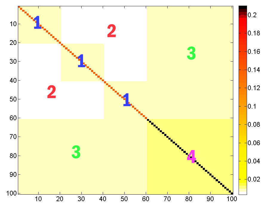
Figure 8: An illustration of the matrix ${\bf B}-{\bf B}_{t,c}^{\textrm{ens}}$ for the ensemble Nyström method where ${\bf B}$ is defined in (9). Here we set $m=100$, $c=20$, $\alpha=0.8$, and $t=3$. For the ensemble Nyström method without overlapping, the matrix ${\bf B}-{\bf B}_{t,c}^{\textrm{ens}}$ can always be partitioned into four regions as annotated.

Based on the properties of the matrix ${\bf B}-{\bf C}^{(i)}{{\bf W}^{(i)}}^{\dagger}{{\bf C}^{(i)}}^{T}$, we study the values of the entries of ${\bf B}-\tilde{{\bf B}}_{t,c}^{\textrm{ens}}$. We can express it as

$${\bf B}-\tilde{{\bf B}}_{t,c}^{\textrm{ens}}={\bf B}-\frac{1}{t}\sum_{i=1}^{t}{\bf C}^{(i)}{{\bf W}^{(i)}}^{\dagger}{{\bf C}^{(i)}}^{T}=\frac{1}{t}\sum_{i=1}^{t}\Big{(}{\bf B}-{\bf C}^{(i)}{{\bf W}}^{\dagger}{{\bf C}^{(i)}}^{T}\Big{)},$$ (45)

and then a discreet examination reveals that ${\bf B}-\tilde{{\bf B}}_{t,c}^{\textrm{ens}}$ can be partitioned into four kinds of regions as illustrated in Figure 8. We annotate the regions in the figure and summarize the values of entries in each region in the table below. (Region 1 and 4 are further partitioned into diagonal entries and off-diagonal entries.)

Region	1 (diag)	1 (off-diag)	2	3	4 (diag)	4 (off-diag)
#Entries	$tc$	$tc^{2}-tc$	$(tc)^{2}-tc^{2}$	$2tc(m-tc)$	$m-tc$	$(m-tc)^{2}-(m-tc)$
Value	$\frac{t-1}{t}(1-\eta)$	$\frac{t-1}{t}(\alpha-\eta)$	$\frac{t-2}{t}(\alpha-\eta)$	$\frac{t-1}{t}(\alpha-\eta)$	$1-\eta$	$\alpha-\eta$

Now we do summation over the entries of ${\bf B}-\tilde{{\bf B}}_{t,c}^{\textrm{ens}}$ to compute its squared Frobenius norm:

$$\big{\|}{\bf B}-\tilde{{\bf B}}_{t,c}^{\textrm{ens}}\big{\|}^{2}_{F} = tc\Big{[}\frac{t-1}{t}(1-\eta)\Big{]}^{2}+\cdots+\big{[}(m-tc)^{2}-(m-tc)\big{]}(\alpha-\eta)^{2}$$

$$= (1-\alpha)(1+\alpha-2\eta)(m-2c+\frac{c}{t})+(\alpha-\eta)^{2}\Big{(}4c^{2}-4cm+m^{2}+\frac{2cm-3c^{2}}{t}\Big{)}$$

$$= (1-\alpha)^{2}\Big{(}m-2c+\frac{c}{t}\Big{)}+\frac{(1-\alpha)^{2}}{(c+\frac{1-\alpha}{\alpha})^{2}}\Big{[}(m-2c+\frac{c}{t})\big{(}\frac{2}{\alpha}-2+m\big{)}+\frac{c(m-c)}{t}\Big{]}$$

$$\geq (1-\alpha)^{2}\Big{(}m-2c+\frac{c}{t}\Big{)}\Big{(}1+\frac{m+\frac{c}{t}+\frac{2}{\alpha}-2}{(c+\frac{1-\alpha}{\alpha})^{2}}\Big{)}\textrm{,}$$

where the last inequality follows from $\frac{c(m-c)}{t}=\frac{c}{t}\Big{(}(m-2c+\frac{c}{t})+(c-\frac{c}{t})\Big{)}\geq\frac{c}{t}\Big{(}m-2c+\frac{c}{t}\Big{)}$.

Furthermore, since the matrices ${\bf B}-{\bf C}^{(i)}{{\bf W}}^{\dagger}{{\bf C}^{(i)}}^{T}$ are all SPSD by Theorem 20, so their sum is also SPSD. Then the SPSD property of $({\bf B}-\tilde{{\bf B}}_{t,c}^{\textrm{ens}})$ follows from (45). Therefore, the nuclear norm of $({\bf B}-\tilde{{\bf B}}_{t,c}^{\textrm{ens}})$ equals to the matrix trace, that is,

$$\big{\|}{\bf B}-\tilde{{\bf B}}_{t,c}^{\textrm{ens}}\big{\|}_{*} = \mathrm{tr}\big{(}{\bf B}-\tilde{{\bf B}}_{t,c}^{\textrm{ens}}\big{)}$$

$$= tc\cdot\frac{t-1}{t}(1-\eta)+(m-tc)\cdot(1-\eta)$$

$$= (1-\alpha)(m-c)\frac{c+\frac{1}{\alpha}}{c+\frac{1-\alpha}{\alpha}}\textrm{,}$$

which proves the nuclear norm bound in the lemma.  

Theorem 24

Assume that the ensemble Nyström method selects a collection of $t$ samples, each sample ${{\bf C}^{(i)}}$ ($i=1,\cdots,t$) contains $c$ columns of ${\bf A}$ without overlapping. For a the matrix ${\bf A}$ defined in (14), the approximation error incurred by the ensemble Nyström method is lower bounded by

$$\big{\|}{\bf A}-\tilde{{\bf A}}_{t,c}^{\textrm{ens}}\big{\|}_{F} \geq (1-\alpha)\sqrt{\Big{(}m-2c+\frac{c}{t}-k\Big{)}+k\bigg{(}\frac{m-c+\frac{c}{t}+k\frac{1-\alpha}{\alpha}}{c+k\frac{1-\alpha}{\alpha}}\bigg{)}^{2}}\textrm{,}$$

$$\big{\|}{\bf A}-\tilde{{\bf A}}_{t,c}^{\textrm{ens}}\big{\|}_{*} \geq (1-\alpha)(m-c)\frac{c+\frac{1}{\alpha}k}{c+\frac{1-\alpha}{\alpha}k}\textrm{,}$$

where $\tilde{{\bf A}}_{t,c}^{\textrm{ens}}=\frac{1}{t}\sum_{i=1}^{t}{\bf C}^{(i)}{{\bf W}^{(i)}}^{\dagger}{{\bf C}^{(i)}}^{T}$.

Proof  According to the construction of ${\bf A}$ in (14), the $i$-th sample ${\bf C}^{(i)}$ is also block diagonal. We denote it by ${\bf C}^{(i)}=\mathsf{BlkDiag}\big{(}\hat{{\bf C}}^{(i)}_{1},\cdots,\hat{{\bf C}}^{(i)}_{k}\big{)}$. Akin to (44), we have

$$\tilde{{\bf A}}_{t,c}^{\textrm{ens}}\;=\;\left[\begin{array}[]{ccc}\frac{1}{t}\sum_{i=1}^{t}\hat{{\bf C}}^{(i)}_{1}\hat{{\bf W}}_{1}^{\dagger}\big{(}\hat{{\bf C}}^{(i)}_{1}\big{)}^{T}&&{\bf 0}\\ &\ddots&\\ {\bf 0}&&\frac{1}{t}\sum_{i=1}^{t}\hat{{\bf C}}^{(i)}_{k}\hat{{\bf W}}_{k}^{\dagger}\big{(}\hat{{\bf C}}^{(i)}_{k}\big{)}^{T}\\ \end{array}\right]\textrm{.}$$

Thus the approximation error of the ensemble Nyström method is

$$\Big{\|}{\bf A}-\tilde{{\bf A}}_{t,c}^{\textrm{ens}}\Big{\|}_{F}^{2} = \sum_{j=1}^{k}\Big{\|}{\bf B}-\frac{1}{t}\sum_{i=1}^{t}\hat{{\bf C}}_{j}^{(i)}\hat{{\bf W}}_{j}^{\dagger}\big{(}\hat{{\bf C}}^{(i)}_{j}\big{)}^{T}\Big{\|}_{F}^{2}$$

$$\geq (1-\alpha)^{2}\sum_{j=1}^{k}\Big{(}p-2{c_{j}}+\frac{{c_{j}}}{t}\Big{)}\Big{(}1+\frac{p+\frac{{c_{j}}}{t}+\frac{2}{\alpha}-2}{({c_{j}}+\frac{1-\alpha}{\alpha})^{2}}\Big{)}$$

$$= (1-\alpha)^{2}\bigg{[}\Big{(}m-2c+\frac{c}{t}\Big{)}+\sum_{j=1}^{k}\Big{(}p-2c_{j}+\frac{c_{j}}{t}\Big{)}\frac{p+\frac{c_{j}}{t}+\frac{2(1-\alpha)}{\alpha}}{(c_{j}+\frac{1-\alpha}{\alpha})^{2}}\bigg{]}\textrm{,}$$

where the inequality follows from Lemma 23, and the last equality follows from $\sum_{j=1}^{k}c_{j}=c$ and $kp=m$. The summation in the last equality equals to

$$\!\!\!\!\!\!\!\!\!\!\!\!\!\!\!\!\!\!\!\!\sum_{j=1}^{k}\bigg{[}\Big{(}p+\frac{c_{j}}{t}+\frac{2(1-\alpha)}{\alpha}\Big{)}-2\Big{(}c_{j}+\frac{1-\alpha}{\alpha}\Big{)}\bigg{]}\frac{p+\frac{c_{j}}{t}+\frac{2(1-\alpha)}{\alpha}}{(c_{j}+\frac{1-\alpha}{\alpha})^{2}}$$

$$\qquad=\;-k+\sum_{j=1}^{k}\bigg{(}\frac{p+\frac{c_{j}}{t}+\frac{2(1-\alpha)}{\alpha}}{c_{j}+\frac{1-\alpha}{\alpha}}-1\bigg{)}^{2}$$

$$\qquad\geq\;-k+k\bigg{(}\frac{m-c+\frac{c}{t}+k\frac{1-\alpha}{\alpha}}{c+k\frac{1-\alpha}{\alpha}}\bigg{)}^{2}\textrm{.}$$

Here the inequality holds because the function is minimized when $c_{1}=\cdots=c_{k}=c/k$. Finally we have that

$$\Big{\|}{\bf A}-\tilde{{\bf A}}_{t,c}^{\textrm{ens}}\Big{\|}_{F}^{2}\;\geq\;(1-\alpha)^{2}\bigg{[}\Big{(}m-2c+\frac{c}{t}-k\Big{)}+k\bigg{(}\frac{m-c+\frac{c}{t}+k\frac{1-\alpha}{\alpha}}{c+k\frac{1-\alpha}{\alpha}}\bigg{)}^{2}\bigg{]}\textrm{,}$$

which proves the Frobenius norm bound in the theorem.

Furthermore, since the matrix ${\bf B}-\frac{1}{t}\sum_{i=1}^{t}\hat{{\bf C}}_{j}^{(i)}\hat{{\bf W}}_{j}^{\dagger}\big{(}\hat{{\bf C}}^{(i)}_{j}\big{)}^{T}$ is SPSD by Lemma 23, so the block diagonal matrix $({\bf A}-\tilde{{\bf A}}_{t,c}^{\textrm{ens}})$ is also SPSD. Thus we have

$$\big{\|}{\bf A}-\tilde{{\bf A}}_{t,c}^{\textrm{ens}}\big{\|}_{*} = (1-\alpha)\sum_{i=1}(p-c_{i})\frac{c_{i}+\frac{1}{\alpha}}{c_{i}+\frac{1-\alpha}{\alpha}}\;\geq\;(1-\alpha)(m-c)\,\Big{(}1+\frac{k}{c+\frac{1-\alpha}{\alpha}k}\Big{)}\textrm{,}$$

which proves the nuclear norm bound in the theorem.  

Theorem 25

Assume that the ensemble Nyström method selects a collection of $t$ samples, each sample ${{\bf C}^{(i)}}$ ($i=1,\cdots,t$) contains $c$ columns of ${\bf A}$ without overlapping. Then there exists an $m{\times}m$ SPSD matrix ${\bf A}$ such that the relative-error ratio of the ensemble Nyström method is lower bounded by

$$\frac{\|{\bf A}-\tilde{{\bf A}}_{t,c}^{\textrm{ens}}\|_{F}}{\|{\bf A}-{\bf A}_{k}\|_{F}} \geq \sqrt{\frac{m-2c+{c}/{t}-k}{m-k}\Big{(}1+\frac{k(m-2c+c/t)}{c^{2}}\Big{)}}\textrm{,}$$

$$\frac{\|{\bf A}-\tilde{{\bf A}}_{t,c}^{\textrm{ens}}\|_{*}}{\|{\bf A}-{\bf A}_{k}\|_{*}} \geq \frac{m-c}{m-k}\>\Big{(}1+\frac{k}{c}\Big{)}\textrm{,}$$

where $\tilde{{\bf A}}_{t,c}^{\textrm{ens}}=\frac{1}{t}\sum_{i=1}^{t}{\bf C}^{(i)}{{\bf W}^{(i)}}^{\dagger}{{\bf C}^{(i)}}^{T}$.

Proof  The theorem follows directly from Theorem 24 and Lemma 19 by setting $\alpha\to 1$.

References

- Ben-Israel and Greville (2003) A. Ben-Israel and T. N. E. Greville. Generalized Inverses: Theory and Applications. Second Edition. Springer, 2003.
- Berry et al. (2005) M. W. Berry, S. A. Pulatova, and G. W. Stewart. Algorithm 844: computing sparse reduced-rank approximations to sparse matrices. ACM Transactions on Mathematical Software, 31(2):252–269, 2005.
- Bien et al. (2010) J. Bien, Y. Xu, and M. W. Mahoney. CUR from a sparse optimization viewpoint. In Advances in Neural Information Processing Systems (NIPS). 2010.
- Bischof and Hansen (1991) C. H. Bischof and P. C. Hansen. Structure-preserving and rank-revealing QR-factorizations. SIAM Journal on Scientific and Statistical Computing, 12(6):1332–1350, 1991.
- Boutsidis et al. (2011) C. Boutsidis, P. Drineas, and M. Magdon-Ismail. Near-optimal column-based matrix reconstruction. CoRR, abs/1103.0995, 2011.
- Chan (1987) T. F. Chan. Rank revealing QR factorizations. Linear Algebra and Its Applications, 88:67–82, 1987.
- Chandrasekaran and Ipsen (1994) S. Chandrasekaran and I. C. F. Ipsen. On rank-revealing factorisations. SIAM Journal on Matrix Analysis and Applications, 15(2):592–622, 1994.
- Cortez et al. (2009) P. Cortez, A. Cerdeira, F. Almeida, T. Matos, and J. Reis. Modeling wine preferences by data mining from physicochemical properties. Decision Support Systems, 47(4):547–553, 2009.
- Deerwester et al. (1990) S. Deerwester, S. T. Dumais, G. W. Furnas, T. K. Landauer, and R. Harshman. Indexing by latent semantic analysis. Journal of The American Society for Information Science, 41(6):391–407, 1990.
- Deshpande and Rademacher (2010) A. Deshpande and L. Rademacher. Efficient volume sampling for row/column subset selection. In Proceedings of the 51st IEEE Annual Symposium on Foundations of Computer Science (FOCS), pages 329–338, 2010.
- Deshpande et al. (2006) A. Deshpande, L. Rademacher, S. Vempala, and G. Wang. Matrix approximation and projective clustering via volume sampling. Theory of Computing, 2(2006):225–247, 2006.
- Drineas and Kannan (2003) P. Drineas and R. Kannan. Pass-efficient algorithms for approximating large matrices. In Proceeding of the 14th Annual ACM-SIAM Symposium on Dicrete Algorithms (SODA), pages 223–232, 2003.
- Drineas and Mahoney (2005) P. Drineas and M. W. Mahoney. On the Nyström method for approximating a gram matrix for improved kernel-based learning. Journal of Machine Learning Research, 6:2153–2175, 2005.
- Drineas et al. (2006) P. Drineas, R. Kannan, and M. W. Mahoney. Fast Monte Carlo algorithms for matrices III: computing a compressed approximate matrix decomposition. SIAM Journal on Computing, 36(1):184–206, 2006.
- Drineas et al. (2008) P. Drineas, M. W. Mahoney, and S. Muthukrishnan. Relative-error CUR matrix decompositions. SIAM Journal on Matrix Analysis and Applications, 30(2):844–881, September 2008.
- Drineas et al. (2012) P. Drineas, M. Magdon-Ismail, M. W. Mahoney, and D. P. Woodruff. Fast approximation of matrix coherence and statistical leverage. In International Conference on Machine Learning (ICML), 2012.
- Foster (1986) L. V. Foster. Rank and null space calculations using matrix decomposition without column interchanges. Linear Algebra and its Applications, 74:47–71, 1986.
- Fowlkes et al. (2004) C. Fowlkes, S. Belongie, F. Chung, and J. Malik. Spectral grouping using the Nyström method. IEEE Transactions on Pattern Analysis and Machine Intelligence, 26(2):214–225, 2004.
- Frank and Asuncion (2010) A. Frank and A. Asuncion. UCI machine learning repository, 2010. URL http://archive.ics.uci.edu/ml.
- Frieze et al. (2004) A. Frieze, R. Kannan, and S. Vempala. Fast Monte Carlo algorithms for finding low-rank approximations. Journal of the ACM, 51(6):1025–1041, November 2004. ISSN 0004-5411.
- Gittens and Mahoney (2013) A. Gittens and M. W. Mahoney. Revisiting the Nyström method for improved large-scale machine learning. arXiv preprint arXiv:1303.1849, 2013.
- Goreinov et al. (1997a) S. A. Goreinov, E. E. Tyrtyshnikov, and N. L. Zamarashkin. A theory of pseudoskeleton approximations. Linear Algebra and Its Applications, 261:1–21, 1997a.
- Goreinov et al. (1997b) S. A. Goreinov, N. L. Zamarashkin, and E. E. Tyrtyshnikov. Pseudo-skeleton approximations by matrices of maximal volume. Mathematical Notes, 62(4):619–623, 1997b.
- Gu and Eisenstat (1996) M. Gu and S. C. Eisenstat. Efficient algorithms for computing a strong rank-revealing QR factorization. SIAM Journal on Scientific Computing, 17(4):848–869, 1996.
- Guruswami and Sinop (2012) V. Guruswami and A. K. Sinop. Optimal column-based low-rank matrix reconstruction. In Proceedings of the 23rd Annual ACM-SIAM Symposium on Discrete Algorithms (SODA), 2012.
- Guyon et al. (2004) I. Guyon, S. Gunn, A. Ben-Hur, and G. Dror. Result analysis of the NIPS 2003 feature selection challenge. Advances in Neural Information Processing Systems (NIPS), 2004.
- Halko et al. (2011) N. Halko, P.-G. Martinsson, and J. A. Tropp. Finding structure with randomness: probabilistic algorithms for constructing approximate matrix decompositions. SIAM Review, 53(2):217–288, 2011.
- Hong and Pan (1992) Y. P. Hong and C. T. Pan. Rank-revealing QR factorizations and the singular value decomposition. Mathematics of Computation, 58(197):213–232, 1992.
- Jin et al. (2011) R. Jin, T. Yang, and M. Mahdavi. Improved bound for the Nyström method and its application to kernel classification. CoRR, abs/1111.2262, 2011.
- Kumar et al. (2009) S. Kumar, M. Mohri, and A. Talwalkar. Ensemble Nyström method. In Advances in Neural Information Processing Systems (NIPS), 2009.
- Kumar et al. (2012) S. Kumar, M. Mohri, and A. Talwalkar. Sampling methods for the Nyström method. Journal of Machine Learning Research, 13:981–1006, 2012.
- Kuruvilla et al. (2002) F. G. Kuruvilla, P. J. Park, and S. L. Schreiber. Vector algebra in the analysis of genome-wide expression data. Genome Biology, 3:research0011–research0011.1, 2002.
- Li et al. (2010) M. Li, J. T. Kwok, and B.-L. Lu. Making large-scale Nyström approximation possible. In International Conference on Machine Learning (ICML), 2010.
- Mackey et al. (2011) L. Mackey, A. Talwalkar, and M. I. Jordan. Divide-and-conquer matrix factorization. In Advances in Neural Information Processing Systems (NIPS). 2011.
- Mahoney (2011) M. W. Mahoney. Randomized algorithms for matrices and data. Foundations and Trends in Machine Learning, 3(2):123–224, 2011.
- Mahoney and Drineas (2009) M. W. Mahoney and P. Drineas. CUR matrix decompositions for improved data analysis. Proceedings of the National Academy of Sciences, 106(3):697–702, 2009.
- Mahoney et al. (2008) M. W. Mahoney, M. Maggioni, and P. Drineas. Tensor-CUR decompositions for tensor-based data. SIAM Journal on Matrix Analysis and Applications, 30(3):957–987, 2008.
- Mesterharm and Pazzani (2011) C. Mesterharm and M. J. Pazzani. Active learning using on-line algorithms. In ACM SIGKDD International Conference on Knowledge Discovery and Data Mining (KDD), 2011.
- Michie et al. (1994) D. Michie, D. J. Spiegelhalter, and C. C. Taylor. Machine learning, neural and statistical classification. 1994.
- Sirovich and Kirby (1987) L. Sirovich and M. Kirby. Low-dimensional procedure for the characterization of human faces. Journal of the Optical Society of America A, 4(3):519–524, Mar 1987.
- Stewart (1999) G. W. Stewart. Four algorithms for the the efficient computation of truncated pivoted QR approximations to a sparse matrix. Numerische Mathematik, 83(2):313–323, 1999.
- Talwalkar and Rostamizadeh (2010) A. Talwalkar and A. Rostamizadeh. Matrix coherence and the Nyström method. arXiv preprint arXiv:1004.2008, 2010.
- Talwalkar et al. (2008) A. Talwalkar, S. Kumar, and H. Rowley. Large-scale manifold learning. In IEEE Conference on Computer Vision and Pattern Recognition (CVPR), 2008.
- Turk and Pentland (1991) M. Turk and A. Pentland. Eigenfaces for recognition. Journal of Cognitive Neuroscience, 3(1):71–86, 1991.
- Tyrtyshnikov (2000) E. E. Tyrtyshnikov. Incomplete cross approximation in the mosaic-skeleton method. Computing, 64:367–380, 2000.
- Williams and Seeger (2001) C. Williams and M. Seeger. Using the Nyström method to speed up kernel machines. In Advances in Neural Information Processing Systems (NIPS), 2001.
- Zhang and Kwok (2010) K. Zhang and J. T. Kwok. Clustered Nyström method for large scale manifold learning and dimension reduction. IEEE Transactions on Neural Networks, 21(10):1576–1587, 2010.
- Zhang et al. (2008) K. Zhang, I. W. Tsang, and J. T. Kwok. Improved Nyström low-rank approximation and error analysis. In International Conference on Machine Learning (ICML), 2008.