Invertible mappings and the large deviation theory for the $q$-maximum entropy principle

Abstract

The possibility of reconciliation between canonical probability distributions obtained from the $q$-maximum entropy principle with predictions from the law of large numbers when empirical samples are held to the same constraints, is investigated into. Canonical probability distributions are constrained by both: $(i)$ the additive duality of generalized statistics and $(ii)$ normal averages expectations. Necessary conditions to establish such a reconciliation are derived by appealing to a result concerning large deviation properties of conditional measures. The (dual) $q^{*}$-maximum entropy principle is shown not to adhere to the large deviation theory. However, the necessary conditions are proven to constitute an invertible mapping between: $(i)$ a canonical ensemble satisfying the $q^{*}$-maximum entropy principle for energy-eigenvalues $\varepsilon_{i}^{*}$, and, $(ii)$ a canonical ensemble satisfying the Shannon-Jaynes maximum entropy theory for energy-eigenvalues $\varepsilon_{i}$. Such an invertible mapping is demonstrated to facilitate an implicit reconciliation between the $q^{*}$-maximum entropy principle and the large deviation theory. Numerical examples for exemplary cases are provided.

PACS numbers

05.20.-y, 02.50.Cw, 05.20.Gg

I Introduction

The generalized (also, interchangeably, nonadditive or deformed) statistics of Tsallis’ has recently been the focus of much attention in complex systems, and allied disciplines 1 (1). The generalized statistics of Tsallis’ is adequate for statistical mechanical systems exhibiting strong correlations and/or long-range interactions. It has generated intense interest in physics and allied disciplines. Many of the issues concerning the properties q-statistics are a subject of intense debate (see, for example 2 (2, 3, 4, 5, 6, 7, 8)), with questions, responses, and counter-responses by many authors. A continually updated bibliography of works related to the generalized statistics of Tsallis may be found at http://tsallis.cat.cbpf.br/biblio.htm.

The large deviation theory constitutes an important statistical basis for information entropies 9 (9, 10). Following the pattern concerning the properties and applicability of the generalized statistics of Tsallis, the adherence of the Tsallis entropy to the large deviation theory has generated considerable interest and debate within the physics community (see, for example 11 (11, 12, 13) and the references therein). In particular, work by La Cour and Schieve 5 (5) showed the canonical probability densities obtained from Tsallis maximum entropy principle to be generally inconsistent with the large deviation theory. The absence of a probabilistic justification for the Tsallis maximum entropy principle has hitherto constituted a significant drawback to the study and utilization of generalized statistics in such formulations.

This paper attempts to reconcile canonical probability distributions obtained from the Tsallis maximum entropy principle with the large deviation theory, based on a procedure that radically differs from that employed in Ref. 5 (5), and utilizing physically realistic expectation values for internal energies (hereinafter referred to as energy expectations). Nonadditive statistics has employed a number of forms in which expectations may be defined. Prominent among these are the linear constraints originally employed by Tsallis 1 (1) (also known as normal averages) of the form: $\left\langle A\right\rangle=\sum\limits_{i}{p_{i}}A_{i}$, the Curado-Tsallis (C-T) constraints 14 (14) of the form: $\left\langle A\right\rangle_{q}=\sum\limits_{i}{p_{i}^{q}}A_{i}\$, and the normalized Tsallis-Mendes-Plastino (TMP) constraints 15 (15) (also known as $q$-averages) of the form: $\left\langle{\left\langle A\right\rangle}\right\rangle_{q}=\sum\limits_{i}{\frac{{p_{i}^{q}}}{{\sum\limits_{i}{p_{i}^{q}}}}A_{i}}\$. Note that in this paper, $<\bullet>$ denotes an expectation. Of these three methods to describe expectations, the most commonly employed by Tsallis-practitioners is the TMP-one.

The originally employed normal averages constraints were abandoned because of serious difficulties in evaluating the partition function. The C-T constraints were replaced by the TMP constraints because they entail the strange relation $\langle 1\rangle_{q}\neq 1$. Recent works by Abe 16 (16, 17, 18) suggest that in generalized statistics expectations defined in terms of normal averages, in contrast to those defined by $q$-averages, are consistent with the generalized H-theorem and the generalized Stosszahlansatz (molecular chaos hypothesis). This resulted in the re-formulation of the variational perturbation approximation in generalized statistics 19 (19).

This paper employs the physically tenable normal averages energy expectations, and specifies the dual Tsallis entropy as the measure of uncertainty. Specifically, it is of essence to utilize the additive duality, defined by re-parameterizing the nonadditive $q$-parameter by specifying: $q\rightarrow 2-q=q^{*}$ 20 (20, 21, 22), when employing normal averages energy expectations. In this instance ”$\rightarrow$” denotes a re-parameterization of the nonadditive parameter, and is not a limit. Application of the additive duality to the Tsallis entropy 1 (1), yields the dual Tsallis entropy:

$$S_{q^{*}}\left[{p_{i}}\right]=-\sum\limits_{i}{p_{i}\ln_{q^{*}}}p_{i},$$ (1)

where the $q^{*}$-logarithm is defined as: $\ln_{q^{*}}x=\frac{{x^{1-q^{*}}-1}}{{1-q^{*}}}$ 23 (23). It is readily seen that in the limit $q^{*}\rightarrow 1$, the dual Tsallis entropy (1) tends to the Shannon entropy.

It is noteworthy to mention that the additive duality was recently employed to successfully demonstrate that the dual generalized Kullback-Leibler divergence is a scaled Bregman divergence 24 (24, 25). This paper derives the necessary conditions to reconcile the dual Tsallis maximum entropy principle with the asymptotic frequencies obtained from large deviation theory (i.e. the law of large numbers), employing normal averages energy expectations. These necessary conditions, which enforce the criterion that the canonical probabilities satisfying the $q^{*}$-maximum entropy principle exactly coincide with those satisfying the Shannon-Jaynes theory, cannot obtained through the analysis in Ref. 5 (5). The $q^{*}$-maximum entropy principle is shown not to explicitly adhere to the large deviation theory.

However, the necessary conditions are demonstrated to constitute an invertible mapping between: $(i)$ a canonical ensemble satisfying the $q^{*}$-maximum entropy principle for energy-eigenvalues $\varepsilon_{i}^{*};i=1,...,m\geq 3$ and parameterized by $\beta^{*}\in[0,\infty]$, and, $(ii)$ a canonical ensemble satisfying the Shannon-Jaynes maximum entropy theory for energy-eigenvalues $\varepsilon_{i};i=1,...,m\geq 3$ and parameterized by $\beta$. The analysis and implications of the invertible mapping, and its role in implicitly reconciling the $q^{*}$-maximum entropy principle with the large deviation theory, is discussed in Sections V-VII of this paper. Note that in Sections V-VII of this paper, the terms necessary conditions and invertible mapping are employed interchangeably. Numerical examples for exemplary cases are provided.

II Dual Tsallis maximum entropy principle

Following the procedure suggested by Ferri, Martinez, and Plastino 26 (26), the canonical probability distribution that maximizes the dual Tsallis entropy for the energy-eigenvalues $\varepsilon_{i}=\{\varepsilon_{i},...,\varepsilon_{m}\},m\geq 3$ subject to the constraint:

$$\sum\limits_{i=1}^{m}{p_{i}\varepsilon_{i}}=u,$$ (2)

and, the normalization constraint: $\sum\limits_{i=1}^{m}{p_{i}}=1$ is:

$$p_{i}=\frac{{\left[{1-\left({1-q^{*}}\right)\beta^{*}\varepsilon_{i}}\right]^{\frac{1}{{1-q^{*}}}}}}{{Z\left({\beta^{*}}\right)}}=\frac{{\exp_{q^{*}}\left[{-\beta^{*}\varepsilon_{i}}\right]}}{{Z\left({\beta^{*}}\right)}},$$ (3)

where: $\left[{1+\left({1-q^{*}}\right)x}\right]^{\frac{1}{{1-q^{*}}}}=\exp_{q^{*}}x$ 23 (23). Here:

$$\begin{array}[]{l}\beta^{*}=\frac{\beta_{q^{*}}}{{\left({2-q^{*}}\right)\beta_{q^{*}}u+\left({1-q^{*}}\right)\aleph_{q^{*}}}};\aleph_{q^{*}}=\sum\limits_{i}{p_{i}^{2-q^{*}}},\\ \\ Z\left({\beta^{*}}\right)=\sum\limits_{i}{\exp_{q^{*}}\left[{-\beta^{*}\varepsilon_{i}}\right]}.\\ \end{array}$$ (4)

Here, $\beta_{q^{*}}$ in (4) is the Lagrange multiplier for the internal energy constraint (2), and $\beta^{*}$ is referred to as the effective inverse temperature. As $q^{*}\rightarrow 1$, $\beta_{q^{*}}\rightarrow\beta$, where $\beta$ is the Boltzmann-Gibbs inverse thermodynamic temperature. Going by the prescription of Ref. 26 (26), instead of canonically evaluating the self-referential expression for $\beta^{*}$, a parametric approach is adopted by a-priori specifying $\beta^{*}\in[0,\infty]$.

Consider a sampling distribution $\mu$. The distribution of frequencies obtained from the random samples $x_{1},...,x_{n}$ tends to $\mu$ as $n\rightarrow\infty$ 5 (5, 9). Let $f_{n,i}(x_{1},...,x_{n})$ be the observed frequency of the discrete energy-eigenvalues $\varepsilon_{i}$ in the sample $x_{1},...,x_{n}$. Thus, (2) may be stated as:

$$\sum\limits_{i=1}^{m}{(\varepsilon_{i}-u)f_{n,i}(x_{1},...,x_{n})}=0.$$ (5)

It will be demonstrated herein that random samples drawn from $\mu$ and satisfying (5) can never give rise to adequate empirical distributions that converge to the dual Tsallis prediction of (3). This is highlighted in Sections IV and VII of this paper. The negative result has prompted the establishment of an implicit adherence of the $q^{*}$-maximum entropy principle to the large deviation theory, facilitated by an invertible mapping described in Sections V-VII of this paper.

III Conditional convergence under constraints

Herein, the convergence in probability of the empirical frequencies $f_{n}=(f_{n,1},...,f_{n,m})$, where $f_{n}$ is a random vector with domain $\left\{{\varepsilon_{1},...,\varepsilon_{m}}\right\}^{n}$ taking values in the convex set $\left\{{p\in\Re^{m};p_{i}>0;\sum\nolimits_{i=1}^{m}{p_{i}}=1}\right\}$, is analyzed. In an unconstrained setting, Sanov’s theorem 5 (5, 9) yields the large deviation rate function for this convergence to be just the negative of the Boltzmann-Gibbs-Shannon entropy and a constant:

$$I_{\mu}\left(p\right)=-S_{q^{*}=1}\left(p\right)-\ln m,$$ (6)

Imposition of additional constraints on $f_{n}$, results in the asymptotic value changing from $\mu$ to a new distribution which minimizes $I_{\mu}$ under the added restrictions 5 (5, 9, 10, 27). For example, imposing the normal averages expectation:

$$\sum\limits_{i=1}^{m}{\varepsilon_{i}f_{n,i}(x_{1},...,x_{n})}=u,$$ (7)

on the sample mean results in an asymptotic distribution which is distinct from $\mu$, and which satisfies $P_{i}\propto e^{-\beta\varepsilon_{i}}$ , where $\beta$ is the Boltzmann-Gibbs inverse thermodynamic temperature. It is ascertained that:

$$\sum\limits_{i=1}^{m}{\varepsilon_{i}P_{i}=u.}$$ (8)

Imposing the condition in (5) yields an asymptotic canonical distribution which minimizes $I_{\mu}$ and maximizes $S_{q^{*}=1}$ subject to the normal averages energy expectations (2):

$$P_{i}=\frac{{\exp\left[{-\beta\varepsilon_{i}}\right]}}{{Z\left(\beta\right)}}.$$ (9)

IV Difference between canonical distributions

The leitmotif of this paper is to derive necessary conditions that allow for agreement between the canonical probabilities $p_{i}$ and $P_{i}$ when $m\geq 3$. To demonstrate this explicitly, the necessary conditions are derived such that for a-priori specified $\beta$ and energy eigenvalues $\varepsilon_{i}=\{\varepsilon_{1},...,\varepsilon_{m}\}$ and specifying $p_{i}=P_{i}$, results in the coincidence of the solutions of (3) and (9) for a state-independent $\beta^{*}\in[0,\infty]$. The difference between the distributions given by (3) and (9) is:

$$d_{i}\left(\beta\right)=\frac{{\exp\left[{-\beta\varepsilon_{i}}\right]}}{{Z\left(\beta\right)}}-\frac{{\exp_{q^{*}}\left[{-\beta^{*}\varepsilon_{i}}\right]}}{{Z\left({\beta^{*}}\right)}},i=1,...,m,\$$ (10)

where:

$$\begin{array}[]{l}Z\left(\beta\right)=\sum\limits_{i=1}^{m}{\exp\left[{-\beta\varepsilon_{i}}\right],}\\ \\ and,\\ \\ Z\left({\beta^{*}}\right)=\sum\limits_{i=1}^{m}{\exp_{q^{*}}\left[{-\beta^{*}\varepsilon_{i}}\right]}.\\ \end{array}$$ (11)

The necessary conditions are obtained by enforcing the condition:

$$d_{i}(\beta)=0;i=1,...,m.$$ (12)

Here, (12) tacitly mandates that the canonical distributions (3) and (9) exactly coincide.

Enforcing the condition in (12), yields:

$$Z^{*}\exp\left[{-\beta\varepsilon_{i}}\right]=\exp_{q^{*}}\left[{-\beta^{*}\varepsilon_{i}}\right];i=1,...,m,\\$$ (13)

where: $Z^{*}=\frac{{Z\left({\beta^{*}}\right)}}{{Z\left(\beta\right)}}>0$. From (13), it is immediately evident that values of $\varepsilon_{i}=0$ result in $Z(\beta^{*})=Z(\beta)$, which is unphysical.

As will be demonstrated in Section VII of this paper, the mapping of (3) onto (9) cannot be achieved for any a-priori state-independent values of $\beta^{*}$ and energy-eigenvalues $\varepsilon_{i},i=1,...,m,m\geq 3$. This tacitly implies that canonical probabilities satisfying the $q^{*}$-maximum entropy principle can never be made to explicitly adhere to the large deviation theory.

V the invertible mapping

To ameliorate this intractable situation, an implicit procedure is adopted to allow for the adherence of canonical probabilities satisfying the $q^{*}$-maximum entropy principle to the large deviation theory. This implicit adherence is accomplished by the introduction of an invertible mapping.

Consider a sampling distribution $\mu^{*}$. The distribution of frequencies obtained from the random samples $x_{1}^{*},...,x_{n}^{*}$. Let $f_{n,i}^{*}(x_{1}^{*},...,x_{n}^{*})$ be the observed frequency of the discrete energy-eigenvalues $\varepsilon_{i}^{*}$ in the sample $x_{1}^{*},...,x_{n}^{*}$. Here, $f_{n}^{*}=(f_{n,1}^{*},...,f_{n,m}^{*})$, where $f_{n}^{*}$ is a random vector with domain $\left\{{\varepsilon_{1}^{*},...,\varepsilon_{m}^{*}}\right\}^{n}$ taking values in the convex set $\left\{{p^{*}\in\Re^{m};p_{i}^{*}>0;\sum\nolimits_{i=1}^{m}{p_{i}^{*}}=1}\right\}$.

The objective of the invertible mapping is to relate: $(i.)$ a canonical ensemble satisfying the $q^{*}$-maximum entropy principle for energy-eigenvalues $\varepsilon_{i}^{*}$ ,with observed frequencies $f_{n,i}^{*}(x_{1}^{*},...,x_{n}^{*})$, and parameterized by a constant $\beta^{*}\in[0,\infty]$, and, $(ii.)$ a canonical ensemble satisfying the Shannon-Jaynes maximum entropy theory for energy-eigenvalues $\varepsilon_{i}$, with observed frequencies $f_{n,i}(x_{1},...,x_{n})$, and parameterized by a constant $\beta$.

For the energy-eigenvalues $\varepsilon_{i}^{*}=\{\varepsilon_{i}^{*},...,\varepsilon_{m}^{*}\},m\geq 3$, (2) and (5) are re-specified as:

$$\sum\limits_{i=1}^{m}{(\varepsilon_{i}^{*}-u)f_{n,i}^{*}(x_{1}^{*},...,x_{n}^{*})}=\sum\limits_{i=1}^{m}{(\varepsilon_{i}^{*}-u)p_{i}^{*}}=0.$$ (14)

Here, (3) is re-defined as:

$$\begin{array}[]{l}p_{i}^{*}=\frac{{\left[{1-\left({1-q^{*}}\right)\beta^{*}\varepsilon_{i}^{*}}\right]^{\frac{1}{{1-q^{*}}}}}}{{Z_{\mu^{*}}\left({\beta^{*}}\right)}}=\frac{{\exp_{q^{*}}\left[{-\beta^{*}\varepsilon_{i}^{*}}\right]}}{{Z_{\mu^{*}}\left({\beta^{*}}\right)}},\\ \\ where,\\ \\ Z_{\mu^{*}}\left({\beta^{*}}\right)=\sum\limits_{i}{\exp_{q^{*}}\left[{-\beta^{*}\varepsilon_{i}^{*}}\right]}.\\ \end{array}$$ (15)

The difference between the distributions given by (15) and (9), is re-defined as:

$$\begin{array}[]{l}d_{i}\left(\beta\right)=\frac{{\exp\left[{-\beta\varepsilon_{i}}\right]}}{{Z\left(\beta\right)}}-\frac{{\exp_{q^{*}}\left[{-\beta^{*}\varepsilon_{i}^{*}}\right]}}{{Z_{\mu^{*}}\left({\beta^{*}}\right)}},i=1,...,m,\\ \\ where:\\ Z\left(\beta\right)=\sum\limits_{i=1}^{m}{\exp\left[{-\beta\varepsilon_{i}}\right],}\\ \\ and,\\ \\ Z_{\mu^{*}}\left({\beta^{*}}\right)=\sum\limits_{i=1}^{m}{\exp_{q^{*}}\left[{-\beta^{*}\varepsilon_{i}^{*}}\right]}.\\ \end{array}$$ (16)

The necessary conditions (13) now acquire the form:

$$Z_{\mu^{*}}^{*}\exp\left[{-\beta\varepsilon_{i}}\right]=\exp_{q^{*}}\left[{-\beta^{*}\varepsilon_{i}^{*}}\right];i=1,...,m,\\$$ (17)

where: $Z_{\mu^{*}}^{*}=\frac{{Z_{\mu^{*}}\left({\beta^{*}}\right)}}{{Z\left(\beta\right)}}>0$. Note that all quantities with the subscript ${\mu^{*}}$, are evaluated for the energy-eigenvalues $\varepsilon_{i}^{*}=\{\varepsilon_{i}^{*},...,\varepsilon_{m}^{*}\}$, and are parameterized by $\beta^{*}$.

By definition:

$$\exp\left[{-\beta\varepsilon_{i}}\right]=Z\left(\beta\right)-\sum\limits_{k\neq i}{\exp\left[{-\beta\varepsilon_{k}}\right]}=Z\left(\beta\right)-\Phi_{i}.\\$$ (18)

Substituting (18) into (17), and taking the $q^{*}$-logarithm on both sides, yields the invertible mapping:

$$\tau_{i}^{*}=\beta^{*}\varepsilon_{i}^{*}=-\ln_{q^{*}}\left[{Z_{\mu^{*}}^{*}\left({Z\left(\beta\right)-\Phi_{i}}\right)}\right];i=1,...,m.$$ (19)

The invertible mapping (19) transforms: $(i.)$ canonical probabilities satisfying the $q^{*}$-maximum entropy principle for energy-eigenvalues $\varepsilon_{i}^{*}$ , and parameterized by a state-independent $\beta^{*}\in[0,\infty]$, into, $(ii.)$ canonical probabilities satisfying the Shannon-Jaynes maximum entropy theory for energy-eigenvalues $\varepsilon_{i}$, and parameterized by a constant $\beta$. Specifically, Eq. (19) invertibly transforms:

$$\frac{{\exp_{q^{*}}\left[{-\beta^{*}\varepsilon_{i}^{*}}\right]}}{{Z_{\mu^{*}}\left({\beta^{*}}\right)}}\ \leftrightarrow\frac{{\exp\left[{-\beta\varepsilon_{i}}\right]}}{{Z\left(\beta\right)}};i=1,...,m.$$ (20)

The objective of the invertible mapping (19) is to evaluate $q^{*}$-canonical probabilities $p_{i}^{*}$ from (15) using the energy-eigenvalues $\varepsilon_{i}^{*}$ parameterized by $\beta^{*}$, and, transform them into Boltzmann-Gibbs canonical probabilities $P_{i}$ defined in (9) in terms of energy-eigenvalues $\varepsilon_{i}$ parameterized by $\beta$. Here, (19) also facilitates the inverse transformation. The leitmotif for this transform is to overcome the formidable obstacles encountered when attempting to explicitly show adherence of the $q^{*}$-maximum entropy principle to the large deviation theory.

Thus, first canonical probabilities $p_{i}^{*}$ are obtained and then transformed into the Boltzmann-Gibbs form $P_{i}$ defined by (9), thereby trivially satisfying (16). In this analysis, (18) is introduced so as to express $\tau_{i}^{*}$ in terms of both the canonical partition function ($Z(\beta)$) and a subset of of it ($\Phi_{i}$) that accounts for contributions of discrete eigenvalues $\varepsilon_{k}$, $k\neq i$.

VI Utility of the invertible mapping

Eq. (9) yields:

$$\begin{array}[]{l}P_{i}=\frac{{\exp\left[{-\beta\varepsilon_{i}}\right]}}{{Z\left(\beta\right)}},\\ \\ {\rm with}\\ \\ Z\left(\beta\right)=\sum\limits_{j=1}^{m}{\exp\left[{-\beta\varepsilon_{j}}\right]},\\ \end{array}$$ (21)

where $i,j=1,...,m$. Taking logarithms in the first relation of (21) yields:

$$\ln P_{i}=-\beta\varepsilon_{i}-\ln Z\left(\beta\right).$$ (22)

The values of $\beta$ and $\ln Z(\beta)$ remain constant $\forall$ $\varepsilon_{i}$ and $\varepsilon_{j}$, and consequently, $\forall$ $P_{i}$ and $P_{j}$;$j\neq i$, $i,j=1,...,m$. Thus, (22) may also be expressed as:

$$\begin{array}[]{l}\ln P_{j}=-\beta\varepsilon_{j}-\ln Z\left(\beta\right)\\ \\ \Rightarrow\beta=-\frac{{\left[{\ln P_{j}+\ln Z\left(\beta\right)}\right]}}{{\varepsilon_{j}}}.\\ \end{array}$$ (23)

Substituting (25) back into the first relation of (23) and re-arranging leads to:

$$\ln Z\left(\beta\right)=\frac{{\varepsilon_{i}\ln P_{j}-\varepsilon_{j}\ln P_{i}}}{{\varepsilon_{j}-\varepsilon_{i}}};i\neq j,i,j=1,...,m.\\$$ (24)

Here, Eq. (24) is readily satisfied for $q^{*}=1$ (Boltzmann-Gibbs canonical probabilities); $\forall i\neq j,i,j=1,...,m,m\geq 3$. Hence the utility of the invertible mapping defined by Eq. (19), which transforms a canonical probability distribution $p_{i}^{*}$ satisfying the $q^{*}$-maximum entropy principle for energy-eigenvalues $\varepsilon_{i}^{*},i=1,...,m$ and parameterized by a constant (state-independent) $\beta^{*}$, to an exactly equivalent Boltzmann-Gibbs canonical probability distribution $p_{i}$ satisfying the Shannon-Jaynes maximum entropy theory for energy-eigenvalues $\varepsilon_{i},i=1,...,m$ and parameterized by a constant $\beta$, and vice-versa.

The analysis in this Section treats two separate and distinct state indices $i$ and $j$; $i\neq j,i,j=1,...,m$. Thus, (19) is re-stated as:

$$\tau_{j}^{*}=\beta^{*}\varepsilon_{j}^{*}=-\ln_{q^{*}}\left[{Z_{\mu^{*}}^{*}\left({Z\left(\beta\right)-\Phi_{j}}\right)}\right];j=1,...,m,$$ (25)

where, $\beta^{*}\in[0,\infty],\forall j$.

The LHS of (24) is required to be the same $\forall i,j,i\neq j$. Invoking (19), (15) acquires the form:

$$\begin{array}[]{l}p_{i}^{*}=\frac{{\exp_{q^{*}}\left[{-\tau_{i}^{*}}\right]}}{{Z_{\mu^{*}}\left({\beta^{*}}\right)}}=\frac{{Z_{\mu^{*}}^{*}\left({Z\left(\beta\right)-\Phi_{i}}\right)}}{{Z_{\mu^{*}}\left({\beta^{*}}\right)}},\\ \\ and,\\ \\ p_{j}^{*}=\frac{{\exp_{q^{*}}\left[{-\tau_{j}^{*}}\right]}}{{Z_{\mu^{*}}\left({\beta^{*}}\right)}}=\frac{{Z_{\mu}^{*}\left({Z\left(\beta\right)-\Phi_{j}}\right)}}{{Z_{\mu^{*}}\left({\beta^{*}}\right)}},\\ \end{array}$$ (26)

$j\neq i;i,j=1,...,m$. Utilizing the relation: $Z_{\mu^{*}}^{*}=\frac{{Z_{\mu^{*}}\left({\beta^{*}}\right)}}{{Z\left(\beta\right)}}$, (26) yields the Boltzmann-Gibbs canonical probability distributions:

$$\begin{array}[]{l}p_{i}=\frac{{\left({Z\left(\beta\right)-\Phi_{i}}\right)}}{{Z\left({\beta}\right)}},\\ \\ and,\\ \\ p_{j}=\frac{{\left({Z\left(\beta\right)-\Phi_{j}}\right)}}{{Z\left({\beta}\right)}},\\ \end{array}$$ (27)

$j\neq i;i,j=1,...,m$. Substituting (27) into (24), yields:

$$\begin{array}[]{l}\ln Z\left(\beta\right)\mathop{\frac{missing}{missing}}{{\varepsilon_{i}\ln\left[{\frac{{Z\left(\beta\right)-\Phi_{j}}}{{Z\left(\beta\right)}}}\right]-\varepsilon_{j}\ln\left[{\frac{{Z\left(\beta\right)-\Phi_{i}}}{{Z\left(\beta\right)}}}\right]}}{{\delta\varepsilon_{ji}}}\\ \\ =\frac{{\varepsilon_{i}\ln\left[{Z\left(\beta\right)-\Phi_{j}}\right]-\varepsilon_{i}\ln Z\left(\beta\right)-\varepsilon_{j}\ln\left[{Z\left(\beta\right)-\Phi_{i}}\right]+\varepsilon_{j}\ln Z\left(\beta\right)}}{{\delta\varepsilon_{ji}}}\\ \\ =\frac{{\varepsilon_{i}\ln\left[{Z\left(\beta\right)-\Phi_{j}}\right]-\varepsilon_{j}\ln\left[{Z\left(\beta\right)-\Phi_{i}}\right]}}{{\delta\varepsilon_{ji}}}+\ln Z\left(\beta\right);\\ \\ \Rightarrow\ln Z(\beta)=\frac{{\varepsilon_{j}\ln\Phi_{i}-\varepsilon_{i}\ln\Phi_{j}}}{{\delta\varepsilon_{ji}}};i,j=1,...,m,i\neq j,\\ \end{array}$$ (28)

where: $\delta\varepsilon_{ji}=\varepsilon_{j}-\varepsilon_{i}$. Expanding (28) with the aid of (18) yields:

$$\begin{array}[]{l}\delta\varepsilon_{ji}\ln Z\left(\beta\right)\\ \\ =\delta\varepsilon_{ji}\ln Z\left(\beta\right)+\varepsilon_{j}\beta\varepsilon_{i}-\varepsilon_{i}\beta\varepsilon_{j}=\delta\varepsilon_{ji}\ln Z\left(\beta\right)\\ \\ \Rightarrow\ln Z\left(\beta\right)=\ln Z\left(\beta\right);i,j=1,...,m,i\neq j.\\ \end{array}$$ (29)

Here, (29) tacitly demonstrates the consistency of the LHS of (24) $\forall i,j=1,...,m;i\neq j$. It is important to note that the identical results to those described in (29) may be obtained by applying the theory described in this paper to the model described in Ref. 5 (5).

VII Implementation of the invertible mapping

The necessary conditions (19) are obtained by enforcing the requirement that the distance between the canonical probability distributions (9) and (15), given by (16), vanishes. This is mandated by Eq. (12) of this paper. The necessary conditions (19) may thus be interpreted as an invertible mapping that transforms (15) into (9). In order that the solutions of (9) coincide with those of (15) for a constant $\beta$, the effective inverse temperature $\beta^{*}$ has to be state-independent $\forall\varepsilon_{i}^{*}$.

This requirement stems from one of the fundamental tenets of statistical physics that in a given canonical ensemble, the energy-eigenvalues constitute a spectrum, but the thermodynamic temperature (or within the context of this analysis, the effective inverse temperature $\beta^{*}$) is fixed, is . Taking the logarithm of (9) for a-priori specified $\beta$ and energy-eigenvalues $\varepsilon_{i},i=1,...,m$, yields:

$$\ln P_{i}=-\beta\varepsilon_{i}-\ln Z\left(\beta\right);i=1,...,m.$$ (30)

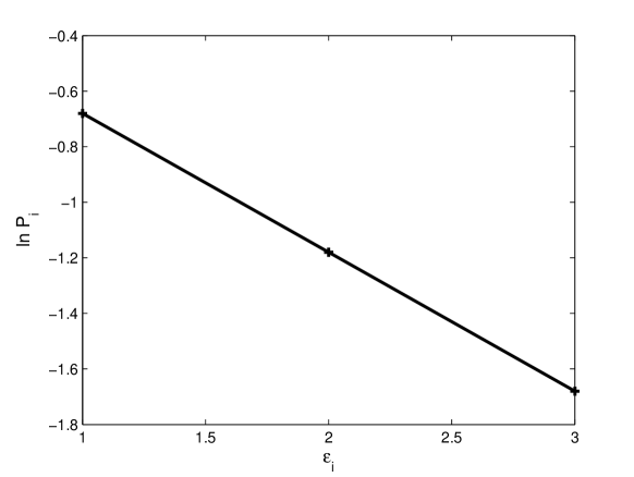
Figure 1: $\varepsilon_{i}=\{1.0,2.0,3.0\},i=1,2,3$ vs. $\ln P_{i}$ from Eq. (30); $\beta=0.5$.

For $\beta=0.5$, $\varepsilon_{i}=\{1.0,2.0,3.0\};i=1,2,3$ versus $\ln P_{i}$, obtained from (30), is a straight line, as is demonstrated in Fig. 1. The value of corresponding canonical partition function, $Z(\beta)$=1.1975. Likewise, taking the logarithm of (15), yields:

$$\ln p_{i}^{*}=\ln\left\{{\exp_{q^{*}}\left[{-\beta^{*}\varepsilon_{i}^{*}}\right]}\right\}-\ln Z_{\mu^{*}}\left({\beta^{*}}\right);i=1,...,m.$$ (31)

For a constant $\beta^{*}\in[0,\infty]$, and energy-eigenvalues $\varepsilon_{i}^{*}=\varepsilon_{i}$, the solutions of (31) cannot coincide with those of (30) for the same canonical ensemble with constant $\beta^{*}$, except perhaps for $m\leq 2$.

For example, even for a simple set of three energy-eigenvalues:$\{\varepsilon_{1},\varepsilon_{2},\varepsilon_{3}\}$, such a coincidence of canonical probabilities for constant $\beta$ and $\beta^{*}$, requires that the following overly prohibitive conditions be simultaneously satisfied:

$$\begin{array}[]{l}\beta^{*}=-\frac{{\ln_{q^{*}}\left\{{Z^{*}\exp\left[{-\beta\varepsilon_{1}}\right]}\right\}}}{\varepsilon_{1}},\\ \\ =-\frac{{\ln_{q^{*}}\left\{{Z^{*}\exp\left[{-\beta\varepsilon_{2}}\right]}\right\}}}{\varepsilon_{2}},\\ \\ =-\frac{{\ln_{q^{*}}\left\{{Z^{*}\exp\left[{-\beta\varepsilon_{3}}\right]}\right\}}}{\varepsilon_{3}}.\\ \end{array}$$ (32)

The derivation of (32) is detailed in the Appendix of this paper.

It is, however, readily demonstrated that the solutions of (31) and (30) will coincide, using the invertible mapping (19). Setting $Z_{\mu^{*}}^{*}=0.9$ in (19) and specifying $\beta^{*}=1.5$, yields the energy-eigenvalues: $\varepsilon_{i}^{*}=\{0.4713,0.9839,1.6420\}$. Here, $Z_{\mu^{*}}(\beta^{*})=1.0778$ for $q^{*}=1.5$. Fig. 2 depicts $\varepsilon_{i}^{*};i=1,2,3$ versus $\ln p_{i}^{*}$. Note that the above mentioned numerical simulation results obey Eq. (32), which is gainfully utilized, by re-stating it in the form:

$$\begin{array}[]{l}\beta^{*}=-\frac{{\ln_{q^{*}}\left\{{Z_{\mu^{*}}^{*}\exp\left[{-\beta\varepsilon_{1}}\right]}\right\}}}{\varepsilon_{1}^{*}},\\ \\ =-\frac{{\ln_{q^{*}}\left\{{Z_{\mu^{*}}^{*}\exp\left[{-\beta\varepsilon_{2}}\right]}\right\}}}{\varepsilon_{2}^{*}},\\ \\ =-\frac{{\ln_{q^{*}}\left\{{Z_{\mu^{*}}^{*}\exp\left[{-\beta\varepsilon_{3}}\right]}\right\}}}{\varepsilon_{3}^{*}},\\ \\ ...\\ \\ =-\frac{{\ln_{q^{*}}\left\{{Z_{\mu^{*}}^{*}\exp\left[{-\beta\varepsilon_{m}}\right]}\right\}}}{\varepsilon_{m}^{*}}.\end{array}$$ (33)

Analytically, the invertible mapping (19) may be readily shown to facilitate the coincidence of (31) with (30) $\forall i=1,...,m;m\geq 3$. Substituting (19) into (31), results in:

$$\begin{array}[]{l}\ln p_{i}^{*}=\ln\exp_{q^{*}}\left\{{\ln_{q^{*}}\left[{Z_{\mu^{*}}^{*}\left({Z\left(\beta\right)-\Phi_{i}}\right)}\right]}\right\}-\ln Z_{\mu^{*}}\left({\beta^{*}}\right)\\ \\ =\ln\left[{Z_{\mu^{*}}^{*}\left({Z\left(\beta\right)-\Phi_{i}}\right)}\right]-\ln Z_{\mu^{*}}\left({\beta^{*}}\right)\\ \\ =\ln Z_{\mu^{*}}^{*}+\ln\left({Z\left(\beta\right)-\Phi_{i}}\right)-\ln Z_{\mu^{*}}\left({\beta^{*}}\right)\\ \\ \mathop{=}\limits^{\left(a\right)}-\beta\varepsilon_{i}-\ln Z\left(\beta\right)\Rightarrow{\rm Eq.(30)~{}recovered!}\end{array}$$ (34)

Here, $(a)$ denotes substituting the expressions: $Z_{\mu^{*}}^{*}=\frac{{Z_{\mu^{*}}\left({\beta^{*}}\right)}}{{Z\left(\beta\right)}}$ and (18), and re-arranging. Thus, (30) is seamlessly recovered from (31) with the aid of the invertible mapping (19). The calculation in (34) does not specify any restriction on the value of $m$.

In the above discussion and the numerical simulations depicted in Fig. 2, $(i)$ $\beta$ and energy-eigenvalues $\varepsilon_{i}$ are given a-priori, $(ii)$ $Z_{\mu^{*}}^{*}$, $\beta^{*}$, and the nonadditive parameter $q^{*}$ are arbitrarily specified, and $(iii)$ the energy-eigenvalues $\varepsilon_{i}^{*}$ are derived from Eq. (19), while ensuring that Eq. (33) is satisfied. It is important to note that the analysis presented herein contains a number of parameters. It is thus imperative to ensure that the fidelity of the invertible mapping (Eq. (19)), which nonlinearly relates $Z_{\mu^{*}}^{*}$, $\beta^{*}$, $\beta$, $\varepsilon_{i}^{*}$, and $\varepsilon_{i}$ is retained, while simultaneously satisfying Eq. (33). A comprehensive multi-parameter study of the invertible mapping is beyond the scope of this paper, and will be presented elsewhere.

VIII Discussions and Conclusions

This paper demonstrates that a given canonical ensemble satisfying the $q^{*}$-maximum entropy principle does not adhere to the large deviation theory. A unique and robust invertible mapping is tacitly demonstrated to facilitate the implicit adherence of a given canonical ensemble satisfying the $q^{*}$-maximum entropy principle, to the large deviation theory.

This is accomplished by: $(i)$ Obtaining canonical probabilities $p_{i}^{*}$ defined by Eq. (15), satisfying the $q^{*}$-maximum entropy principle for energy-eigenvalues $\varepsilon_{i}^{*}=\{\varepsilon_{1}^{*},...,\varepsilon_{m}^{*}\};m\geq 3$, and parameterized by a state-independent effective inverse temperature $\beta^{*}\in[0,\infty]$, $(ii)$ Utilizing the invertible mapping described by Eq. (19) to obtain canonical probabilities satisfying the Shannon-Jaynes maximum entropy theory for energy-eigenvalues $\varepsilon_{i}=\{\varepsilon_{1},...,\varepsilon_{m}\};m\geq 3$, and parameterized by a constant inverse thermodynamic temperature $\beta$, and, $(iii)$ demonstrating that the difference between the canonical probabilities (Eq. (16)) is trivially satisfied, thereby proving an implicit adherence of the $q^{*}$-maximum entropy principle to the large deviation theory.

This is specifically accomplished by mapping a canonical ensemble that satisfies $q^{*}$-maximum entropy principle but does not adhere to the large deviation theory, onto, a canonical ensemble that satisfies the Shannon-Jaynes theory whose foundations are intimately intertwined to the large deviation theory 9 (9, 10, 27). Note that the invertible mapping (Eq. (19)) seamlessly allows for the interchange of steps $(i)$ and $(ii)$ described above, depending upon the energy-eigenvalues and other parameters made available.

Numerical results for exemplary cases have been provided. The results presented in this paper constitute a substantial qualitative improvement vis-á-vis those demonstrated in previous studies, that have attempted to reconcile the $q$-maximum entropy principle with the large deviation theory. A comprehensive analysis of the invertible mapping (Eq.(19)), from information geometric considerations, is currently being pursued. This analysis also assesses the sensitivity of the invertible mapping to variations in $Z_{\mu^{*}}^{*}$, $\beta^{*}$, $\beta$, $\varepsilon_{i}^{*}$, and $\varepsilon_{i}$. The pertinent results will be presented elsewhere.

Appendix A Derivation of Eq. (32)

For simplicity, a set of three energy-eigenvalues:$\{\varepsilon_{1},\varepsilon_{2},\varepsilon_{3}\}$ is chosen, which satisfy the Shannon-Jaynes maximum entropy theory. From $q$-algebra (Ref. 23 (23)), the following relation is obtained:

$$\begin{array}[]{l}\exp_{q^{*}}\left[x\right]\otimes_{q^{*}}\exp_{q^{*}}\left[y\right]=\exp_{q^{*}}\left[{x+y}\right],\\ \\ where:\\ \\ x\otimes_{q^{*}}y=\left[{x^{1-q^{*}}+y^{1-q^{*}}-1}\right]^{\frac{1}{{1-q^{*}}}};x,y>0.\\ \end{array}$$ (35)

The discrete set of energy-eigenvalues may be denoted as: $\{\varepsilon_{1},\varepsilon_{1}+\delta_{1},\varepsilon_{1}+\delta_{2}\}$, where $\delta_{1},\delta_{2}>0$. Setting:

$$\tau_{1}^{*}=-\beta^{*}\varepsilon_{1},\tau_{1}=-\beta\varepsilon_{1},\delta\tau_{1}^{*}=-\beta^{*}\delta_{1},and,\delta\tau_{1}=-\beta\delta_{1}.$$ (36)

Substituting $(A.2)$ into $(A.1)$, Eq. (13) yields with application of $q$-algebra:

$$\begin{array}[]{l}\exp_{q^{*}}\left[{\tau_{1}^{*}+\delta\tau_{1}^{*}}\right]=\exp_{q^{*}}\left[{\tau_{1}^{*}}\right]\otimes_{q^{*}}\exp_{q^{*}}\left[{\delta\tau_{1}^{*}}\right]\\ \\ \Rightarrow\left\{{\left({\exp_{q^{*}}\left[{\tau_{1}^{*}}\right]}\right)^{1-q^{*}}+\left({\exp_{q^{*}}\left[{\delta\tau_{1}^{*}}\right]}\right)^{1-q^{*}}-1}\right\}^{\frac{1}{{1-q^{*}}}}\\ \\ =Z^{*}\exp\left[{\tau_{1}+\delta\tau_{1}}\right]\\ \\ \Rightarrow 1-\left({1-q^{*}}\right)\beta^{*}\left({\varepsilon_{i}+\delta_{1}}\right)=[Z^{*}\exp\left[{\tau_{1}+\delta\tau_{1}}\right]]^{1-q^{*}}\\ \\ \Rightarrow\beta^{*}=-\frac{{\ln_{q^{*}}\left\{{Z^{*}\exp\left[{-\beta\left({\varepsilon_{1}+\delta_{1}}\right)}\right]}\right\}}}{{\varepsilon_{1}+\delta_{1}}}.\\ \end{array}$$ (37)

For consistency of the constant values of $\beta^{*}$, $\beta$, and $Z^{*}$, it is required that:

$$\begin{array}[]{l}\beta^{*}=-\frac{{\ln_{q^{*}}\left\{{Z^{*}\exp\left[{-\beta\varepsilon_{1}}\right]}\right\}}}{{\varepsilon_{1}}}=-\frac{{\ln_{q^{*}}\left\{{Z^{*}\exp\left[{-\beta\left({\varepsilon_{1}+\delta_{1}}\right)}\right]}\right\}}}{{\varepsilon_{1}+\delta_{1}}},\\ \\ and\\ \\ \beta^{*}=-\frac{{\ln_{q^{*}}\left\{{Z^{*}\exp\left[{-\beta\varepsilon_{1}}\right]}\right\}}}{{\varepsilon_{1}}}=-\frac{{\ln_{q^{*}}\left\{{Z^{*}\exp\left[{-\beta\left({\varepsilon_{1}+\delta_{2}}\right)}\right]}\right\}}}{{\varepsilon_{1}+\delta_{2}}}\\ \end{array}$$ (38)

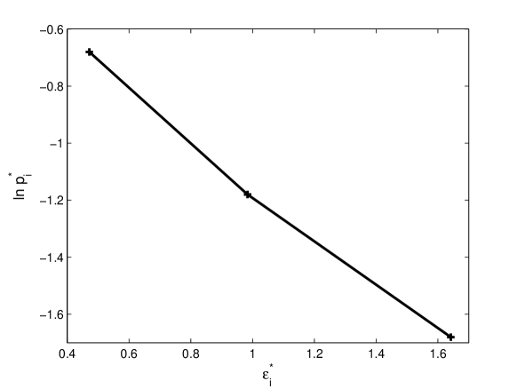
Figure 2: $\varepsilon_{i}^{*}=\{0.4713,0.9839,1.6420\}$ vs. $\ln p_{i}^{*}$ from Eq. (31); $\beta^{*}=1.5,q^{*}=1.5$.

References

• (1) C. Tsallis, Introduction to Nonextensive Statistical Mechanics: Approaching a Complex World, (Springer-Verlag, New York, 2009).
• (2) D. H.Β Zanette and M. M.Β Montemurro, Phys. Lett. A 316, 194 (2003).
• (3) D. H.Β Zanette and M. M.Β Montemurro, Phys. Lett. A 324, 383 (2004).
• (4) E.Β Vives and A.Β Planes, Phys. Rev. Lett. 88, 02061 (2002).
• (5) B.Β R.Β La Cour and W.Β C.Β Schieve, Phys. Rev. E 62, 7494 (2000).
• (6) F.Β Bouchet, T.Β Dauxois, and S.Β Ruffo, Europhys. News 37, 9 (2008).
• (7) B.Β H.Β Lavenda and J.Β Dunning-Davies, J. Appl. Sci. 5, 315 (2005).
• (8) M.Β Nauenberg, Phys. Rev. E 67, 036114 (2003).
• (9) R.Β S. Ellis, Entropy, Large Deviations, and Statistical Mechanics, (Springer-Verlag, New York, 1985).
• (10) H.Β Touchette, Phys. Rep. 478, 1 (2009).
• (11) G.Β Ruiz, and C.Β Tsallis, Phys. Lett. A 376, 2451 (2012).
• (12) H.Β Touchette, Phys. Lett. A 377, 436 (2013).
• (13) G.Β Ruiz, and C.Β Tsallis, Phys. Lett. A 377, 377 (2013).
• (14) E.Β M.Β F.Β Curado, and C.Β Tsallis, J. Phys. A: Math Gen. 24, L91 (1991).
• (15) C.Β Tsallis, R. S.Β Mendes, and A.Β R.Β Plastino, Physica A 261, 524 (1998).
• (16) S.Β Abe, Phys. Rev. E 79, 04116 (2009).
• (17) S.Β Abe, Europhys. Lett. 84, 60006 (2008).
• (18) S.Β Abe, J. Stat. Mech.: Th. Expt. , P07027 (2009).
• (19) R. C.Β Venkatesan, and A.Β Plastino, Physica A 389, 1159 (2010);Physica A 389, 2155 (2010).
• (20) T.Β Wada, and A. M.Β Scarfone, Eur. Phys. Jour. B 47, 557 (2005).
• (21) T.Β Wada, and A. M.Β Scarfone, Phys. Lett. A. 335, 351 (2005).
• (22) J.Β Naudts, Physica A 340, 32 (2004).
• (23) E.Β Borges, Physica A 340, 95 (2004).
• (24) R. C.Β Venkatesan, and A.Β Plastino, Physica A 390, 2749 (2011).
• (25) R. C.Β Venkatesan, and A.Β Plastino, Phys. Lett. A 375, 4237 (2011);Phys. Lett. A 376, 3470 (2012).
• (26) G. L.Β Ferri, S.Β Martinez, and A.Β Plastino, J. Stat. Mech.: Th. Expt. , P04009 (2005).
• (27) R. S.Β Ellis, Physica D 133, 106 (1999). *