Forces between a partially coherent fluctuating source and a magnetodielectric particle.

Abstract

We address the forces exerted by the electromagnetic field emitted by a planar fluctuating source on dielectric particles that have arose much interest because of their recently shown magnetodielectric behavior. In this context, we analyze as a particular case the modification of the Casimir and Van der Waals forces. We study the effect of the source coherence length as well as the interplay between the force from the radiated field and that from the electric and magnetic dipoles induced on the particle. This allows a control of these interactions as well as of the weight and interference effects between the fields from both kinds of induced dipoles, in particular when large changes in their differential scattering cross section occur due to Kerker minimum forward or zero backward conditions; thus opening new paths to nanoparticle ensembling and manipulation. The influence of surface waves of the source is also studied.

Magnetodielectric particles have recently attracted much attention due to their exotic properties as scatterers and nanoantennas (Novotny and van Hulst, 2011; Mehta et al., 2006; Liu et al., 2012; Schuller et al., 2010; Rolly et al., 2012; Schuller et al., 2007; Kerker et al., 1983; Kuznetsov et al., 2012; Evlyukhin et al., 2012). It has been shown (García-Etxarri et al., 2011; Fan et al., 2010) that some dielectric particles behave in this way exhibiting coupled electric and magnetic dipoles induced by the illuminating light field. It is then of great interest to study their response to stochastic radiation forces, specifically those due the field of a planar fluctuating source (Mandel and Wolf, 1995). Many previous studies have dealt with this subject for atoms or non-magnetic nanoparticles with its application to delta-correlated thermal sources and blackbodies in connection with the Van der Waals (VdW) and Casimir-Polder (C-P) interactions (Henkel et al., 2002; Antezza et al., 2005; Novotny and Henkel, 2008).

In this work we deal with a more general kind of statistical sources, namely those that are spatially partially coherent and of the wide variety of those statistically homogeneous and isotropic (Mandel and Wolf, 1995; Auñón and Nieto-Vesperinas, 2012a). Their emission excites electric and magnetic dipoles of the particle in its near field that may be considered as a secondary source whose radiation interacts with the primary fluctuating source; this giving rise to a new total force resulting from both the action of the field radiated by the primary source and that from the field emitted by these dipoles. At thermal wavelengths, the interaction from this secondary source constituted by the particle induced dipoles is interpreted as a Liftshitz force (Lifshitz, 1956), which at zero temperature becomes either those derived by VdW and C-P (Casimir and Polder, 1948), depending on the distance and use, or not, of quasistatic formulations. However, in our study, first the optical wavelengths are such that $\hbar\omega/kT>>1$ and hence Planck energy becomes similar to that of the vacuum fluctuations: $\hbar\omega[\frac{1}{2}+1/(\exp(\hbar\omega/kT)-1)]\approx\frac{1}{2}\hbar\omega$; and second, due to the magnetic response of the nanoparticle, more forces come into play in addition to those that keep an analogy with these above quoted, thus allowing a larger number of degrees of freedom of relevance for particle ensembling and manipulation. We do not restrict here to thermal wavelengthts, but rather consider a range of infrared and optical frequencies whose choice depends on the particle size. Then a particular case of our study is that analogous to those dipole forces induced by spontaneous electromagnetic field fluctuations. While the vacuum forces can become relatively negligible by conveniently manipulating the power intensity of the source, we shall show that in other possible configurations and experimental designs they may predominate.

The geometry considered in this letter consists of two half-spaces. The lower one ($z<0$) is occupied by the source with its polarization currents and it will be denoted as $1$; whereas the upper one ($z>0$), denoted as $2$, is free space and contains the particle.

The Cartesian components of the force on a magnetodielectric dipolar particle is the sum of an electric, magnetic and electric-magnetic dipole interference parts which are expressed in terms of the first electric and magnetic Mie coefficients $a_{1}$ and $b_{1}$ as (Nieto-Vesperinas et al., 2010)

$$F_{i}\left(\mathbf{r}\right) = F_{i}^{e}\left(\mathbf{r}\right)+F_{i}^{m}\left(\mathbf{r}\right)+F_{i}^{e-m}\left(\mathbf{r}\right)$$ (1)

$$= \frac{\varepsilon_{0}\varepsilon_{2}}{2}\text{Re}\left\{\left\langle\alpha_{e}E_{j}^{*}\left(\mathbf{r}\right)\partial_{i}E_{j}\left(\mathbf{r}\right)\right\rangle\right\}$$

$$+ \frac{\mu_{0}\mu_{2}}{2}\text{Re}\left\{\left\langle\alpha_{e}H_{j}^{*}\left(\mathbf{r}\right)\partial_{i}H_{j}\left(\mathbf{r}\right)\right\rangle\right\}$$

$$- \varepsilon_{0}\varepsilon_{2}\frac{Zk_{0}^{4}}{12\pi}\text{Re}\left\{\left(\alpha_{e}^{*}\alpha_{m}\right)\left\langle\mathbf{E}^{*}\times\mathbf{H}\right\rangle_{i}\right\},$$

where $i,j=1,2,3$, $\varepsilon_{l}=\varepsilon_{l}^{\prime}+i\varepsilon_{l}^{\prime\prime}$ and $\mu_{l}=\mu_{l}^{\prime}+i\mu_{l}^{\prime\prime}$ $(l=1,2)$ are the permittivity and susceptibility of the medium embedding the particle, respectively, in our case being vacuum; and $Z=\sqrt{\mu_{0}\mu_{1}/\varepsilon_{0}\varepsilon_{1}}$. $\alpha_{e}$ and $\alpha_{m}$ standing for the electric and magnetic polarizability of the particle, respectively. $\alpha_{e}=i\frac{3\epsilon_{0}}{2k^{3}}a_{1}$, $\alpha_{m}=i\frac{3}{2\mu_{0}k^{3}}b_{1}$; $E_{i}(\bf{r})$ is the total electric vector at frequency $\omega$ at any point of the half-space $z>0$, hence at the position of the particle, i.e. at $\mathbf{r}=\mathbf{r}_{0}$, it will be

$$E_{i}(\mathbf{r}_{0}) = E_{i}^{inc}(\mathbf{r}_{0})+E_{i}^{p}(\mathbf{r}_{0})+E_{i}^{m}(\mathbf{r}_{0})$$ (2)

$$= E_{i}^{inc}+\mu_{0}\mu_{2}\omega^{2}G_{ij}^{p}p_{j}+i\mu_{0}\mu_{2}\omega G_{ij}^{m}m_{j}.$$

In the second line of this equation we have omitted the explicit dependency on space and frequency for brevity. The associated magnetic field can be obtained directly from Maxwell’s equations. In Eq. (2) the last two terms are the electric fields emitted by the particle induced dipoles ($p_{i}=\varepsilon_{0}\alpha_{e}E_{i}^{inc}$ and $m_{i}=\alpha_{m}H_{i}^{inc}$) after multiple reflections at the plane $z=0$ (Wylie and Sipe, 1984) and hence connect the constitutive properties of the source and particle through the reflection Fresnel coefficients $r_{s,p}$ at $z=0$ and the polarizabilities, being described by $G_{ij}^{p,m}$. On the other hand, the first term $E_{i}^{inc}$ represents the electric field incident on the particle after being emitted from the primary source placed at $z<0$, and is defined through the Green’s function $G_{ij}^{P}$ which includes the transmission Fresnel coefficients $t_{s,p}$ from $z<0$ into $z>0$. $G_{ij}^{P}$ may be written as a superposition of plane waves with wavevector $k_{0}\mathbf{s}_{i}=k_{0}(\mathbf{s_{\perp}},s_{z,i})$ with $\mathbf{s_{\perp}}=(s_{x},s_{y})$, $s_{z,i}^{2}=\varepsilon_{i}\mu_{i}-s_{\perp}^{2}$,($i=1,2$), and $k_{0}=2\pi/\lambda=\omega/c$. Thus, in terms of the polarization currents one has

$$E_{i}^{inc}\left(\mathbf{r}_{0}\right)=\mu_{0}\mu_{2}\omega^{2}\int_{V}G^{P}_{ij}\left(\mathbf{r}_{0},\mathbf{r}^{\prime},\omega\right)P_{j}\left(\mathbf{r}^{\prime},\omega\right)d^{3}r^{\prime}.$$ (3)

In vacuum ($\varepsilon_{2}=\mu_{2}=1$), $G_{ij}^{p,m}$ decays exponentially with the distance in the evanescent wave region ($s_{\perp}>1$) and is oscillatory in the radiative one ($s_{\perp}<1$)(Novotny and Hecht, 2006). For a single dipole, this electric field is calculated from Eq. (3) using $G_{ij}^{p}$ and $p_{i}\delta({\bf r}^{\prime}-{\bf r}_{0})$ instead of $G_{ij}^{P}$ and $P_{j}({\bf r}^{\prime})$. In a similar way, the electric field $E^{m}$ generated by the magnetic dipole can be calculated from the Green function associated to the magnetic field of the electric dipole $H^{p}$ and making the interchange $r^{s}\leftrightarrow r^{p}$ in the reflection Fresnel coefficients. Some details about these Green’s functions can be found in e.g. (Sipe, 1987; Joulain et al., 2005). Note that for p-polarization, both $t_{p}$ and $r_{p}$ support surface plasmon polaritons (SPPs) when $\varepsilon_{2}^{\prime}<1$.

Now we define the cross-spectral density tensor of the source polarization as $W_{ij}^{(P)}\left(\mathbf{r}_{1},\mathbf{r}_{2},\omega\right)=\left\langle P_{i}^{*}\left(\mathbf{r}{}_{1},\omega\right)P_{j}\left(\mathbf{r}{}_{2},\omega\right)\right\rangle$. We shall address the wide variety of non-local statistically homogeneous and isotropic sources (Mandel and Wolf, 1995)) for which

$$W_{ij}^{(P)}(\mathbf{r}_{1},\mathbf{r}_{2},\omega)=S^{(P)}(\omega)\mu_{ij}^{(P)}(|\mathbf{r}_{1}-\mathbf{r}_{2}|,\omega).$$ (4)

$S^{P}(\omega)$ denotes the power spectrum of the source and $\mu_{ij}(\mathbf{r}_{1},\mathbf{r}_{2},\omega)$ is the spectral degree of coherence (Mandel and Wolf, 1995). A special particular case of these sources are those thermal and blackbodies widely studied. On inserting Eq. (2) into (1) and taking the statistical homogeneity of the source into account, one obtains the total force on the particle. For these sources only the force along the $z$-axis is different from zero. We consider mutual incoherence between the particle electric and magnetic induced dipoles, i.e., $\left\langle p_{i}^{*}m_{j}\right\rangle=0$ (Rytov et al., 1989). $F_{1}$ and $F_{2}$ will denote the total forces due to the above mentioned contributions of the primary fluctuating source in $z<0$ and to the secondary source field from the particle induced dipoles, respectively.

We study the effect of the magnetodielectric properties of the particle in the near infrared. This is a semiconductor sphere; its anomalous scattering properties have recently received a great deal of attention, both theoretically and experimentally (Nieto-Vesperinas et al., 2011; Geffrin et al., 2012; Fan et al., 2010; Liu et al., 2012). In particular, for each incident plane wave component its scattered intensity in the backscattering direction is zero, [first Kerker condition ($K1$)] when $\text{Re}{\alpha_{e}}=\text{Re}{\alpha_{m}}$ is fulfilled. Also for each of such plane wave components impinging the particle, the forwardly scattered intensity becomes close to a non-zero minimum [second Kerker condition (K2)] when $\text{Re}{\alpha_{e}}=-\text{Re}{\alpha_{m}}$ . In both cases: $\text{Im}{\alpha_{e}}=\text{Im}{\alpha_{m}}$ (Nieto-Vesperinas et al., 2011).

Thus, we address a Si sphere of radius $a=230nm$, the spectrum of the incident light being in the range of $1.2-2\mu m$. At these frequencies the total cross section of the particle is fully determined by the Mie coefficients $a_{1}$ and $b_{1}$ (García-Etxarri et al., 2011), this justifies the use of Eq. (1).

We assume a Gaussian degree of coherence of the source, therefore the correlation function reads $W_{ij}^{(P)}\left(\mathbf{r}_{1},\mathbf{r}_{2},\omega\right)$ $={\cal S}^{(P)}\left(\omega\right)\text{exp}\left(-\left(\left|\mathbf{r}_{1}-\mathbf{r}_{2}\right|\right)^{2}/2\sigma^{2}\right)\delta_{ij}/(2\pi)^{3/2}\sigma^{3}$, $\sigma$ being the coherence length of the source and $S^{(P)}(\omega)={\cal S}^{(P)}(\omega)/(2\pi)^{3/2}\sigma^{3}$ representing the normalized spectrum. Notice that for $\sigma\rightarrow 0$, $W^{(P)}_{ij}(\mathbf{r}_{1},\mathbf{r}_{2},\omega)={\cal S}^{(P)}(\omega)\delta(|\mathbf{r}_{1}-\mathbf{r}_{2}|,\omega)\delta_{ij}$, then the source becomes $\delta$-correlated, like in e.g. a thermal one following the fluctuation-dissipation theorem (Rytov et al., 1989). The source considered here will have an Au interface at $z=0$, hence supporting surface plasmons polaritons (SPPs) in the spectral range under consideration, and thus enhancing the near field forces Auñón and Nieto-Vesperinas (2012b). After performing all the integrations of the form of Eq. (3) for the primary source and for the induced dipoles, (a long but straightforward work, some of whose details are shown in the supplementary information), one sees that $\left\langle E_{i}^{m*}(\mathbf{r}_{0})E_{i}^{m}(\mathbf{r}_{0})\right\rangle=\left\langle H_{i}^{p*}(\mathbf{r}_{0})E_{i}^{p}(\mathbf{r}_{0})\right\rangle=0$. This will be relevant when we discuss the particle Kerker conditions.

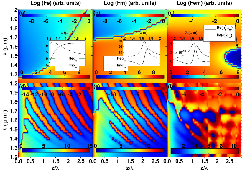
Figure 1: (Color online). From left to right: Normalized electric ($F^{e}$), magnetic ($F^{m}$) and interference force ($F^{em}$) from a $\delta$-correlated source. The first horizontal row shows the part of the force due to the field from the fluctuating primary source at $z=0$, [first term in Eq. (2)]. The insets exhibit the behavior of the electric, magnetic and electric-magnetic interaction force components, respectively, normalized to $a^{3}$. The second horizontal row represents the force from the secondary source constituted by the particle induced dipoles, [second and third terms in Eq. (2)]

Fig. 1 shows the logarithm of the force. This representation aims to clarifying its drastic changes of sign. All the results of this paper will be normalized to the spectrum of the source in order to see the relative weight of each force component. The first horizontal row shows the force $F_{1}$ due to the field impinging from the primary statistical source at $z=0$. The second horizontal row represents the force $F_{2}$ from the secondary source constituted by the electric and magnetic dipoles induced on the particle. The fluctuating source coherence length $\sigma$ is first assumed to be zero. The inset shows the behavior of the polarizability for the range of wavelengths considered. This helps to understand the color plots. In Figs. 1(a) and 1(b) we see a line separating the gradient and scattering forces. For a statistically homogeneous source, the gradient force (proportional to $\text{Re}{\alpha_{e}}\left\langle E_{i}^{*}E_{i}\right\rangle$) is governed uniquely by the evanescent modes and is negative for a particle with $\text{Re}\alpha_{e}>0$ (Auñón and Nieto-Vesperinas, 2012b), hence, it exponentially decays with the distance z to the source. On the other hand, the scattering force (proportional to $\text{Im}{\alpha_{e}}\text{Im}{\left\langle E_{j}^{*}\partial_{i}E_{j}\right\rangle}$) is positive, i.e. pushing, and constant for any $\mathbf{r}_{0}$. As the wavelength grows, $\text{Re}\alpha_{e}>\text{Im}\alpha_{e}$, [see the inset in Fig. 1(a)], the gradient force dominates even at distances larger than $\lambda$, where the evanescent modes do not contribute. This is a remarkable new feature of this kind of particles. Fig. 1 (c) represents the force component $F_{i}^{e-m}$ due to interference between the particle induced electric and magnetic dipoles. In the near field this is almost repulsive for any wavelength, however, at distances larger than the wavelength, where the Poynting vector $\mathbf{S}=\text{Re}(\mathbf{E^{*}}\times\mathbf{H})/2$ is independent of the distance, we have a zone where this force is negative (the arrow indicates that zone). This kind of action is known as a pulling force (Chen et al., 2011; Sukhov and Dogariu, 2011; Novitsky et al., 2011), and its interest has increased in the last years. This last plot shows the relevant role of the magnetodielectric behavior of these particles in this respect, although in this latter specific case when the two other components: electric and magnetic, are added this pulling effect becomes very small, (the electric-magnetic dipole interference force at $\lambda\simeq 1.47\mu m$ and $z\geq 2.5\lambda$ is one order of magnitude less than either $F_{1}^{e}$ or $F_{1}^{m}$), however by manipulating the fluctuating source, a suitable power of the emitted electromagnetic field is obtained (Novotny and Henkel, 2008) so that a tractor light field appears, even in the far zone.

Concerning the force $F_{2}$ fom the particle induced dipoles, we observe in the second row of Fig. 1 that this force exponentially decays with the distance z to the primary source plane $z=0$, and its sign depends on that of the particle polarizability; nevertheless, the oscillating behavior of the Green function due to propagating plane wave components manifests in this force. We also observe that it is six orders of magnitude larger than its counterpart $F_{1}$ from the primary fluctuating source, at least at subwavelength distances $z$. We shall later discuss this.

To get a deeper understanding, Fig. 2 represents $F_{2}$ for some selected wavelengths and for two different source coherence lengths: $\sigma=0$ and $\sigma=\lambda/4$. For an statistically homogeneous source, the relationship between the electric and magnetic cross-spectral density tensors is (Jouttenus et al., 2005)

$$\varepsilon_{0}\left\langle E_{i}^{*}(\mathbf{r}_{1},\omega)E_{j}(\mathbf{r}_{2})\right\rangle=\mu_{0}\left\langle H_{i}^{*}(\mathbf{r}_{1},\omega)H_{j}^{*}(\mathbf{r}_{2})\right\rangle,$$ (5)

hence, in the near field, when the first or the second Kerker condition holds, one has $F^{e}_{1}=F^{m}_{1}$ and $F^{e}_{1}=-F^{m}_{1}$, however, in the far zone $F^{e}_{1}=F^{m}_{1}$ for any value of $\mathbf{r}_{0}$. For the Si particle addressed, the Kerker conditions are fullfilled at $\lambda_{1}\simeq 1.825\mu m$ and $\lambda_{2}\simeq 1.53\mu m$, (see Figs. 2(a) and 2(b) and (Nieto-Vesperinas et al., 2011)). We can also see in the inset of Fig. 1(b), that in the range of $\lambda=1.6-1.65\mu m$ there is a peak in the imaginary part of $\alpha_{m}$ which predominates over all other $\alpha$ parts. The black-dashed-dot line in Fig. 2 represents the force in this peak. In that case, the magnetic force $F^{m}_{z,1}$ is one order of magnitude larger than $F^{e}_{z,1}$ and $F^{em}_{z,1}$, hence the total force on the particle is governed by this magnetic force. This effect, due to the dielectric particle magnetic response to the light field, constitutes one of the main results of this paper.

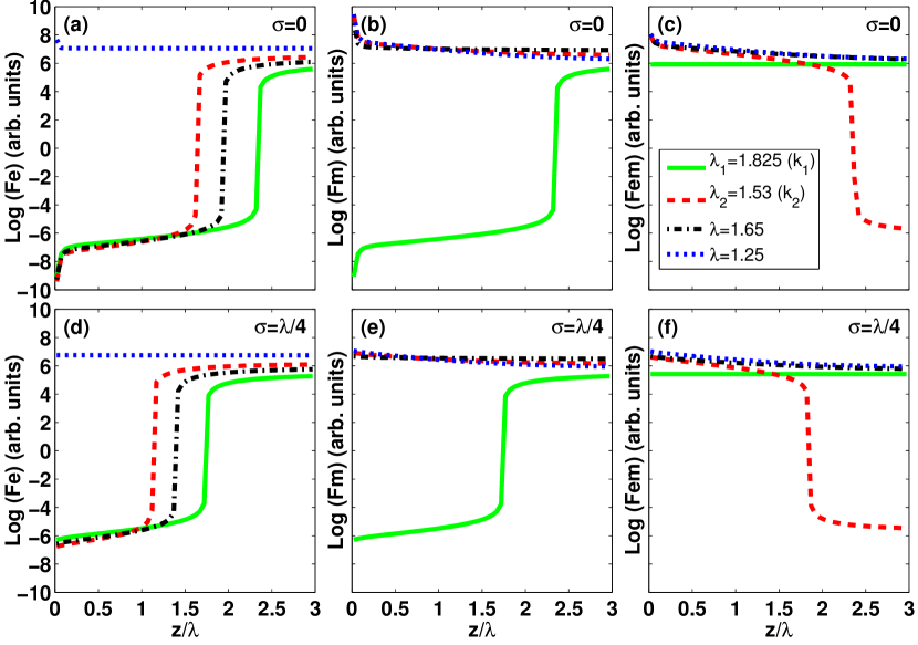
Figure 2: (Color online). Normalized $F_{1}^{e}$, $F_{1}^{m}$ and $F_{1}^{em}$ versus the distance from the plane of the source (in wavelength units) for some values of the wavelength (in $\mu m$). The two Kerker conditions occur at $\lambda_{1}$, (K1), and $\lambda_{2}$, (K2), respectively.

We now address the influence of the coherence length of the source. This will establish the differences between the mechanical action of partially correlated sources and that from e.g. thermal sources and blackbodies. The spectral degree of coherence in $k-$space is $\exp[-(k\sigma s_{\perp})^{2}/2]$, hence, it acts a low-pass filter being maximum for $\sigma=0$ (i.e. when the source is $\delta$-correlated). Because of this fact, the evanescent modes present two such filters: the first is due to the own nature of these evanescent modes while the second stems from the spatial coherence of the source. The shape of Figs. 2(d)-(f) is similar to that of Figs. 2(a)-(c), shifted by a distance $\Delta z\simeq 0.5\lambda$, therefore for $\sigma>\lambda$ the force is solely due to the non-conservative (scattering) force and to the interference force $F_{1}^{em}$, which becomes constant and positive or negative depending on the wavelength. It is worth pointing out that the price paid on increasing the coherence length is expensive, because at the same time there is a reduction of the force strength by various orders of magnitude [cf. e.g. the forces shown in Figs. 2 (a) and 2 (d)].

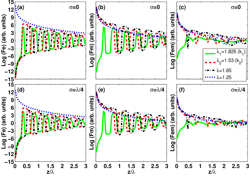
Figure 3: Color online). Normalized $F_{2}^{e}$, $F_{2}^{m}$ and $F_{2}^{em}$ versus distance $z$ (in units of wavelength) from the exit plane $z=0$ of the source for different values of the wavelength (in $\mu m$). The two Kerker conditions are fulfilled at $\lambda_{1}$, (K1), and $\lambda_{2}$, (K2), respectively.

Once we understood the role of the coherence length, we turn our study to its influence on the force $F_{2}$ induced by the secondary source, namely by the particle induced dipoles. Fig. 3 represents $F_{2}$ for the same wavelengths as in Fig. 2. The magnitude of the force in the near-field $z<\lambda$ is much larger than in Fig. 2, thus, the effect of the mechanical action $F_{2}$ of the field emitted by the particle induced dipoles substantially dominates over that $F_{1}$ of the field that is due solely to the stochastic source. Nevertheless, as the distance $z$ grows, all the fastly oscillating components, electric, magnetic and that of interference, of this force $F_{2}$ rapidly tend to zero, and hence is the force $F_{1}$ from the primary source the one that dominates. As follows from the calculation of $E^{p,m}$ and $H^{p,m}$, the cross spectral density tensor of the electric and magnetic dipoles now are not equal; therefore, and although at first sight it could seem that similar relationships between the electric and magnetic forces, in Kerker conditions, are fulfilled like for $F_{1}$ from the primary source, in fact they are not.

The role of the coherence length in this case is exactly the same as in Fig. 1; the magnitude of the force decreases as $\sigma$ grows. Future work should find a minimum value of $\sigma$ for which the Casimir-Polder force predominates over the contributions discussed here.

In summary, we have shown, that the mechanical action on a magnetodielectric small particle from a partially coherent fluctuating source exhibits important new effects at distances shorter than the wavelength. In particular, the magnetic induced dipole and its interference with the electric dipole create a landscape of forces completely different to that previously studied in connection with Van der Waals, Casimir, Liftshitz and rest of radiation forces both in and out of thermodynamic equilibrium. In this respect, Kerker conditions, as a result of the exotic scattering properties of these particles, introduce new relationships in the balance of these new forces over the traditional purely electric forces. Further experiments should be stimulated by these new effects, including consequences of Fano resonances.

References

- Novotny and van Hulst (2011) L. Novotny and N. van Hulst, Nature Photonics 5, 83 (2011).
- Mehta et al. (2006) R. V. Mehta, R. Patel, R. Desai, R. V. Upadhyay, and K. Parekh, Phys. Rev. Lett. 96, 127402 (2006).
- Liu et al. (2012) W. Liu, A. E. Miroshnichenko, D. N. Neshev, and Y. S. Kivshar, ACS Nano 6, 5489 (2012).
- Schuller et al. (2010) J. A. Schuller, E. S. Barnard, W. Cai, Y. C. Jun, J. S. White, and M. L. Brongersma, Nature materials 9, 193 (2010).
- Rolly et al. (2012) B. Rolly, B. Stout, and N. Bonod, Opt. Express 20, 20376 (2012).
- Schuller et al. (2007) J. A. Schuller, R. Zia, T. Taubner, and M. L. Brongersma, Phys. Rev. Lett. 99, 107401 (2007).
- Kerker et al. (1983) M. Kerker, D.-S. Wang, and C. L. Giles, J. Opt. Soc. Am. 73, 765 (1983).
- Kuznetsov et al. (2012) A. I. Kuznetsov, A. E. Miroshnichenko, Y. H. Fu, J. Zhang, and B. Luk’yanchuk, Scientific Reports 2 (2012).
- Evlyukhin et al. (2012) A. B. Evlyukhin, S. M. Novikov, U. Zywietz, R. L. Eriksen, C. Reinhardt, S. I. Bozhevolnyi, and B. N. Chichkov, Nano Letters 12, 3749 (2012), http://pubs.acs.org/doi/pdf/10.1021/nl301594s .
- García-Etxarri et al. (2011) A. García-Etxarri, R. Gómez-Medina, L. S. Froufe-Pérez, C. López, L. Chantada, F. Scheffold, J. Aizpurua, M. Nieto-Vesperinas, and J. J. Sáenz, Opt. Express 19, 4815 (2011).
- Fan et al. (2010) X. Fan, Z. Shen, and B. Luk’yanchuk, Opt. Express 18, 24868 (2010).
- Mandel and Wolf (1995) L. Mandel and E. Wolf, Optical Coherence and Quantum Optics (Cambridge U. Press, Cambridge, UK, 1995).
- Henkel et al. (2002) C. Henkel, K. Joulain, J.-P. Mulet, and J.-J. Greffet, Journal of Optics A: Pure and Applied Optics 4, S109 (2002).
- Antezza et al. (2005) M. Antezza, L. P. Pitaevskii, and S. Stringari, Phys. Rev. Lett. 95, 113202 (2005).
- Novotny and Henkel (2008) L. Novotny and C. Henkel, Opt. Lett. 33, 1029 (2008).
- Auñón and Nieto-Vesperinas (2012a) J. M. Auñón and M. Nieto-Vesperinas, J. Opt. Soc. Am. A 29, 1389 (2012a).
- Lifshitz (1956) E. Lifshitz, Sov. Phys. JETP 2, 73 (1956).
- Casimir and Polder (1948) H. B. G. Casimir and D. Polder, Phys. Rev. 73, 360 (1948).
- Nieto-Vesperinas et al. (2010) M. Nieto-Vesperinas, J. J. Sáenz, R. Gómez-Medina, and L. Chantada, Opt. Express 18, 11428 (2010).
- Wylie and Sipe (1984) J. M. Wylie and J. E. Sipe, Phys. Rev. A 30, 1185 (1984).
- Novotny and Hecht (2006) L. Novotny and B. Hecht, Principles of nano-optics (Cambridge university press, 2006).
- Sipe (1987) J. E. Sipe, J. Opt. Soc. Am. B 4, 481 (1987).
- Joulain et al. (2005) K. Joulain, J.-P. Mulet, F. Marquier, R. Carminati, and J.-J. Greffet, Surface Science Reports 57, 59 (2005).
- Rytov et al. (1989) S. M. Rytov, Y. A. Kravtsov, and V. I. Tatarskii, Principles of statistical radiophysics. Part 3: elements of Random Fields (Springer-Verlag, Berlin, 1989).
- Nieto-Vesperinas et al. (2011) M. Nieto-Vesperinas, R. Gomez-Medina, and J. J. Sáenz, J. Opt. Soc. Am. A 28, 54 (2011).
- Geffrin et al. (2012) J. Geffrin, B. García-Cámara, R. Gómez-Medina, P. Albella, L. Froufe-Pérez, C. Eyraud, A. Litman, R. Vaillon, F. González, M. Nieto-Vesperinas, J. Sáenz, and F. Moreno, Nature Communications 3, 1171 (2012).
- Auñón and Nieto-Vesperinas (2012b) J. M. Auñón and M. Nieto-Vesperinas, Phys. Rev. A 85, 053828 (2012b).
- Chen et al. (2011) J. Chen, J. Ng, Z. Lin, and C. T. Chan, Nature Photon. 5, 531 (2011).
- Sukhov and Dogariu (2011) S. Sukhov and A. Dogariu, Phys. Rev. Lett. 107, 203602 (2011).
- Novitsky et al. (2011) A. Novitsky, C. W. Qiu, and H. Wang, Phys. Rev. Lett. 107, 203601 (2011).
- Jouttenus et al. (2005) T. Jouttenus, T. Setälä, M. Kaivola, and A. T. Friberg, Phys. Rev. E 72, 046611 (2005).