Surface reflectance of Mars observed by CRISM/MRO: 2. Estimation of surface photometric properties in Gusev Crater and Meridiani Planum

Abstract: The present article proposes an approach to analyze the photometric properties of the surface materials from multi-angle observations acquired by the Compact Reconnaissance Imaging Spectrometer for Mars (CRISM) on-board the Mars Reconnaissance Orbiter. We estimate photometric parameters using Hapke’s model in a Bayesian inversion framework. This work also represents a validation of the atmospheric correction provided by the Multi-angle Approach for Retrieval of Surface Reflectance from CRISM Observations (MARS-ReCO) proposed in the companion article.The latter algorithm retrieves photometric curves of surface materials in reflectance units after removing the aerosol contribution. This validation is done by comparing the estimated photometric parameters to those obtained from in situ measurements by Panoramic Camera instrument at the Mars Exploration Rover (MER)-Spirit and MER-Opportunity landing sites. Consistent photometric parameters with those from in situ measurements are found, demonstrating that MARS-ReCO gives access to accurate surface reflectance. Moreover the assumption of a non-Lambertian surface as included in MARS-ReCO is shown to be significantly more precise to estimate surface photometric properties from space in comparison to methods based on a Lambertian surface assumption. In the future, the presented method will allow us to map from orbit the surface bidirectional reflectance and the related photometric parameters in order to characterize the Martian surface.

1 Introduction

Reflectance of planetary surfaces is tightly controlled by the composition of the present materials but also by their granularity, the internal heterogeneities, porosity, and roughness. The reflectance can be characterized by measurements at different wavelengths, viewing geometries (emergence direction) and solar illuminations (incidence direction). Such investigations have been conducted for Mars using telescopes, instruments on-board spacecrafts and rovers. A summary of these studies is available in the Johnson et al. (2008) review chapter. One can find studies related to: the Viking Landers (Guinness et al., 1997), the Pathfinder Lander (Johnson et al., 1999), the Hubble Space Telescope (Bell III et al., 1999), the PANoramic CAMera (Pancam) instrument on-board Mars Exploration Rovers (MER) (Johnson et al., 2006a, b), the Observatoire pour la Minéralogie, l’Eau, les Glaces et l’Activité (OMEGA) instrument on-board Mars Express (MEx) (Pinet et al., 2005) and the High Resolution Stereo Camera (HRSC) instrument on-board MEx (Jehl et al., 2008). Recently, Shaw et al. (2012) derived maps of mm- to cm- scale surface roughness at MER-Opportunity landing site by using multi-angle hyperspectral imager spectrometer called Compact Reconnaissance Imaging Spectrometer for Mars (CRISM) on-board Mars Reconnaissance Orbiter (MRO).

In order to derive compositional and structural information from reflectance measurements, physical models describing the interaction of light with natural media are needed. Chandrasekhar (1960) proposed the radiative transfer equation describing the loss and gains of multidirectional streams of radiative energy within media considered as continuously absorbing and scattering where grains are separated by a distance greater than the wavelength (e.g. atmospheres). In the case of a dense medium (e.g., surfaces), two different solutions are developed. First, solutions based on Monte Carlo ray tracing methods handled the medium complexity (e.g. Grynko and Shkuratov, 2007). Unfortunately, this direct approach requires large computing times and large parameter space, limiting the inversion. Second, solutions based on an empirical or semi-empirical approach were proposed by adapting the radiative transfer equation to granular media (e.g., Hapke, 1981a, b, 1986, 1993, 2002; Shkuratov and Starukhina, 1999; Douté and Schmitt, 1998). These techniques are more relevant for inversion. Several parameters characterize natural surfaces such roughness and compaction, while other parameters characterize an average grain, such the single scattering albedo or the phase function.

Previous photometric studies suggest that variations in scattering properties are controlled by local processes. For example, photometric variations observed by Pancam at Columbia Hill and the cratered plains of Gusev Crater are mainly caused by aeolian and impact cratering processes (Johnson et al., 2006a). These conclusions encourage us to expand the estimation of photometric properties from in situ observations to the entire planet using orbital data to go further in the interpretations.

Observations acquired from space, however, require the correction for atmospheric contribution (i.e., gases and aerosols) in the remotely sensed signal prior to the estimation of the bidirectional reflectance of the surface materials. Previous orbital photometric studies of Martian surfaces were conducted without atmospheric correction but using the lowest aerosols content observations (e.g., Jehl et al., 2008; Pinet et al., 2005). Using data acquired by the multi-angle hyperspectral imaging spectrometer called CRISM on-board MRO (Murchie et al., 2007), our objective is to estimate accurate (i) surface bidirectional reflectance of the surface of Mars and (ii) photometric parameters associated with the materials. Ceamanos et al. (2013) presents a method referred to as Multi-angle Approach for Retrieval of Surface Reflectance from CRISM Observations (MARS-ReCO). This original technique takes advantage of the multi-angular capabilities of CRISM to determine the bidirectional reflectance of the Martian surface. This is done through the atmospheric correction of the signal sensed at the top of atmosphere (TOA). We propose an approach to analyze the photometric parameters of the surface materials in terms of structural information by inverting Hapke’s photometric model in a Bayesian framework, as discussed below. The validation of the methods proposed in this work and in the companion article (Ceamanos et al., 2013) is performed by comparing the estimated photometric parameters to those obtained from in situ measurements by Pancam instrument at the MER-Spirit and MER-Opportunity landing sites (respectively at Gusev Crater and Meridiani Planum) (Johnson et al., 2006a, b).

This article is organized as follows. First, the methodology to obtain photometric surface parameters is described in Section 2. Second, the estimated photometric parameters are presented in Section 3. Third, results are compared to experimental studies, independent orbital measurements and in situ measurements in Section 4. The significance of the photometric results shall be discussed in Section 5.

2 Methodology

This article and its companion take advantage of the multi-angular capabilities of the CRISM instrument to correct for atmospheric contribution in order to estimate the surface bidirectional reflectance (Ceamanos et al., 2013) and to determine the surface photometric parameters (this work). The approach presented in this article includes the following steps: (i) the selection of appropriate CRISM observations at both MER landing sites for the photometric study, (ii) the determination of the surface bidirectional reflectance by correcting for aerosol contributions, (iii) the combination of several CRISM observations for a better sampling of the surface bidirectional reflectance, and (iv) the estimation of the associated surface photometric parameters. The detailed scheme of the procedure is illustrated in Figure 1. One should note that, in order to test the performance of the method presented throughout this article and its companion paper, the study is only conducted at one wavelength and for some spatial pixels. We choose to work at 750 nm where (i) the contribution of gases is minimal and thus the retrieval of photometric properties is likely to be more accurate and (ii) in situ photometric measurements from Pancam instrument are available for the comparison to the estimated photometric parameters.

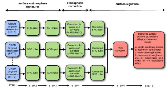
Figure 1: Detailed scheme of the estimation of surface photometric properties. The blue blocks represent the initial FRT CRISM observations (from $i$=1 to n). The green blocks represent the aerosol optical thickness retrieval and the correction for atmospheric contribution for the determination of the surface bidirectional reflectance, which is carried out by the methodology described in the companion paper (Ceamanos et al., 2013). The red blocks correspond to the work presented in this article, that is the estimation of surface photometric properties.

2.1 CRISM data sets

2.1.1 The CRISM instrument and targeted observations

The CRISM instrument on-board MRO is a visible and infrared hyperspectral imager (i.e. 362 to 3920 nm at 6.55 nm/channel) that operates from a sun-synchronous, near-circular (255 x 320 km altitude), near-polar orbit since November 2006. The appropriate mode to estimate surface spectrophotometric properties is the so-called targeted mode providing Full Resolution Targeted (FRT) observations consisting of a sequence of eleven hyperspectral images from a single region acquired at different emission angles. The solar incidence angle is almost constant during the MRO flyby of a targeted observation. A typical targeted sequence is composed of a nadir image ($\sim$10x10 km) at high spatial resolution (15-19 m/pixel) and ten off nadir images with a 10x-spatial binning (resulting in a resolution of 150-200 m/pixel) taken before and after the nadir image. The latter sequence constitutes the so-called Emission Phase Function (EPF) sequence. The pointing of CRISM can rotate (gimbal) ± 60° (Murchie et al., 2007).

2.1.2 Selection of targeted observations

As explained in the companion paper (Ceamanos et al., 2013), the accuracy of the surface reflectance provided by MARS-ReCO when dealing with a single targeted observation highly depends on the combination of a moderate atmospheric opacity (i.e. aerosol optical thickness less than or equal to 2), reasonable illumination conditions (i,e. incidence angle less than or equal 60°), an appropriate phase domain (i.e. significant difference between the available maximum and minimum phase angles up to 40°) and on the number and diversity of angular measurements. The combination of several targeted observations, since it enables a better sampling of the bidirectional reflectance, could therefore significantly improve the reflectance estimation as it provides more regular angular sampling of the surface target. Pinet et al. (2005) and Jehl et al. (2008) proved the benefits of using different spaceborne observations under varied illumination conditions (OMEGA and HRSC). The principal requirement to combine targeted observations is the absence of seasonal changes among the selected observations.

Several CRISM observations have been acquired over the MER landing sites since the beginning of the mission. In particular, up to sixteen and ten CRISM full targeted observations (FRT) are available in the MER-Spirit and MER-Opportunity landing sites, respectively. In this article, we select CRISM observations according to several criteria: (i) the quality of overlap among the observations (above 70%), (ii) the variation of the solar incidence angle implying a widening of the phase angle domain (note that only the variation of the seasonal solar longitude ($Ls$) can provide different incidence angles due to the sun-synchronous orbit of MRO, and (iii) the absence of surface changes (e.g., seasonal phenomena) as they can jeopardize the determination of the surface photometric properties. Taking into account these criteria, three CRISM observations acquired over Gusev Crater (i.e., FRT3192, FRT8CE1 and FRTCDA5) and over Meridiani Planum (i.e., FRT95B8, FRT334D and FRTB6B5) are selected, respectively. We note that the selected observations have quite different phase angle ranges as shown in Table 1.

Table 1: Selected CRISM observations focused on the Spirit and Opportunity landing sites, respectively at Gusev Crater and Meridiani Planum. $Ls$, stands for the solar longitude, $\theta_{0}$ is the incidence angle, $g$ is the phase angle range. AOT_mineral stands for the mineral Aerosol Optical Thickness at 1 $\mu m$ from Wolff’s estimates (Wolff et al., 2009) (personal communication of Michael Wolff) and AOT_water is the water Aerosol Optical Thickness at 320 nm by MARs Color Imager instrument (personal communication of Michael Wolff).

	Gusev Crater (MER-Spirit)			Meridiani Planum (MER-Opportunity)
	FRT3192	FRT8CE1	FRTCDA5	FRT95B8	FRT334D	FRTB6B5
Acquisition date	2006-11-22	2007-12-17	2008-10-07	2008-01-11	2006-11-30	2008-07-08
$Ls$ (degree)	139.138	4.040	138.333	16.223	142.975	96
$\theta_{0}$ (degree)	60.4	40.02	62.8	39.3	55.4	56.4
$g$ (degree)	$\sim$56-112	$\sim$41-90	$\sim$46-106	$\sim$41-86	$\sim$41-106	$\sim$40-106
AOTmineral (1$\mu m$)	0.33$\pm$0.04	0.98$\pm$0.15	0.32$\pm$0.04	0.56$\pm$0.09	0.35$\pm$0.04	0.35$\pm$0.04
AOTwater (320 nm)	0.08$\pm$0.03	0.07$\pm$0.03	0.03$\pm$0.03	0.12$\pm$0.05	0.12$\pm$0.03	0.14$\pm$0.03

Targeted observations are archived in the Planetary Data System (PDS) and are composed of: (i) Targeted Reduced Data Records (TRDR), which store the calibrated data in units of I/F (radiance factor - RADF, see Table 2), the ratio of measured intensity to solar flux, and (ii) Derived Data Records (DDR), which store the ancillary data such as the spatial coordinates (latitude and longitude) and the geometric configurations of each pixel by means of the incidence, emission and phase angles. In the present study, CRISM products are being released with the TRDR2 version of CRISM calibration (TRR2 for brevity).

Table 2: Photometric units derived from the bidirectional reflectance $r$. ($I$: intensity, $F$: solar flux, : $\theta_{0}$: incidence angle, $\theta$: emergence angle, $g$: phase angle). The CRISM observations are released in RADF unit and the SPC cubes in BRF units.

	Unit	Symbol	Name	Expression
reflectance	$sr^{-1}$	$r$	bidirectional reflectance	$r\left(\theta_{0},\theta,g\right)=\frac{I}{\pi\times F}$
		$BRDF$	bidirectional reflectance distribution function	$BRDF=r(\theta_{0},\theta,g)/\cos\left(\theta_{0}\right)$
		$RADF$	Radiance factor	$RADF=\pi\times r(\theta_{0},\theta,g)=\frac{I}{F}$
		$BRF$	bidirectional reflectance factor	$\rho=BRF=\pi\times r(\theta_{0},\theta,g)/\cos\left(\theta_{0}\right)$

2.1.3 SPC cubes: Integrated multi-angle product

To facilitate the access to the multi-angular information pertaining to each terrain unit, the eleven hyperspectral images corresponding to a single targeted observation were spatially rearranged into data set named SPC (spectro-photometric curve) cube (see Ceamanos et al. (2013) for more detail). The SPC cube is composed of: (i) $x$ dimension (horizontal) corresponding to angular configurations (up to eleven) grouping all reflectance values at different geometric views, (ii) $y$ dimension (vertical) corresponding to the spatial coordinate defining a super-pixel. The super-pixels are rearranged as function of the number of available angular configurations and, (iii) $z$ dimension corresponding to the spectral sampling. The photometric curves, stored in a SPC cube are in units of RADF (see Table 2), correspond to the signals TOA. In the present work, all selected FRT observations are binned at 460 meters per pixel (the spatial resolution of each super-pixel). This is done (i) to cope with the geometric deformation inaccuracies in the case of an oblique view with pointing errors, (ii) to minimize on poorly known topography (a CRISM pixel is smaller than MOLA resolution), (iii) to reduce local seasonal variations and (iv) to minimize local slopes effects. We found that binning at 460 meters is a good compromise.

2.2 Estimation of surface bidirectional reflectance: Correction for atmospheric contribution

The radiative transfer in the Martian atmosphere is dominated by CO₂ and H₂O gases, mineral and ice aerosols which are an obstacle for the studies of the surface properties. Indeed the extinction of radiative fluxes, in particular the solar irradiance in the wavelength range of CRISM observations, is mostly due to absorption by gases and scattering by aerosols. Also, aerosols produce an additive signal by scattering of the solar light. As a result, a spectrum collected by the CRISM instrument at the Top Of-Atmosphere (TOA) is a complex signal determined by both the surface and the atmospheric components (gases and aerosols). The atmospheric correction chain proposed for CRISM observations is composed of: (i) the retrieval of Aerosol Optical Thickness (AOT), (ii) the correction for gases, and (iii) the correction for aerosols resulting in the estimation of the surface reflectance. The last step is carried out by the technique referred to as the MARS-ReCO (Ceamanos et al., 2013). In the following, a short summary of the methodology is provided.

2.2.1 Retrieval of AOT

The AOT is defined as the aerosol optical depth along the vertical of the atmosphere layer and is related to the aerosol content.

The retrieval of AOT from orbit is difficult because of the coupling of signals between the aerosols and the surface. Over the last decades, Emission Phase Function (EPF) sequences of Mars were obtained and were used to separate the atmospheric and surface contributions. Significant progresses have resulted from the pioneer works of Clancy and Lee (1991) based on Viking orbiter InfraRed Thermal Mapper (IRTM) EPF observations and Clancy et al. (2003) from Mars Global Surveyor (MGS) Thermal Emission Spectrometer (TES) EPF observations ten years later.

For our study, we decided to use Michael Wolff’s AOT estimates for atmospheric correction purposes (personal communication). This parameter is available for each CRISM observation and is derived from Wolff et al. (2009)’s work. This method is based on the analysis of CRISM EPF sequences combined with information provided by “ground truth” results at both MER landing sites which allow to isolate the single scattering albedo. This method carries out a minimization of the mean square error between measured and predicted TOA radiance based on the previously estimated aerosol single scattering albedo and scattering phase function.

Some assumptions regarding the aerosol properties (i.e., phase function, mixing ratio, column optical depth, etc) and the surface properties (i.e., phase function) must have been accounted for to separate the atmospheric and surface contributions. Concerning the surface properties, this method assumes a non-Lambertian surface to estimate the AOT by using a set of surface photometric parameters that appears to describe the surface phase function adequately for both MER landing sites (Johnson et al., 2006a, b). This assumption is qualitative but reasonable for several reasons enumerated by Wolff et al. (2009). For both MER landing sites it seems from Wolff et al. (2009)’s work that the AOT retrievals are overall consistent with optical depths returned by the Pancam instrument (available via PDS). Consequently, the Wolff’s AOT estimates are suitable for our study at both MER landing sites. Concerning the aerosol properties, some uncertainties may exist especially for the aerosol scattering phase function which is related to the aerosol particle size and shape. First, this method assumes a mean particle aerosol but variations are observed as a function of solar longitude, spatial location (latitude, longitude and altitude) (Wolff et al., 2006). Second the mean aerosol particle size is derived from CRISM observations acquired during planet-encircling dust event in 2007. During a large dust event, aerosol particle size are larger than those found under clear atmospheric conditions. Third, the hypothesis of the particle shape used in Wolff et al. (2009)’s study contain a wrong backscattering part in the scattering phase function (Wolff et al., 2010). Thus all points previously enumerated, may bias the AOT estimation and must be taken into account during the analysis of the robustness of results (the surface bidirectional reflectance and the surface photometric parameters). However, the performance of MARS-ReCO is sensitive to the accuracy of the AOT estimate (Ceamanos et al., 2013) (see 2.2.2).

Note that the AOT is calculated at 1 $\mu m$ where the absorption of gases is almost null.

2.2.2 Correction for gases and aerosols

In order to test the performances of the methodology presented in this article and its companion paper, the present study is only conducted at a single wavelength. We choose to work exclusively at 750 nm where the contribution of gases is low and thus the retrieval of photometric properties is likely to be sufficiently accurate. Furthermore, photometric properties retrieved from in situ measurements taken by Pancam are available at this wavelength and our photometric properties can be validated. Note, however, that the presented methodology can be applied to any CRISM wavelength provided the contribution of gases is corrected previously.

MARS-ReCO is devised to compensate for mineral aerosol effects considering the anisotropic scattering properties of the surface and the aerosols. This method is suitable for any CRISM multi-angle observation within some atmospheric and geometrical constraints (AOT$\leq$2, incidence angle $\theta_{0}$<60°, phase angle range $g{}_{max}-g_{min}$>40°). MARS-ReCO is based on a coupled surface-atmosphere radiative transfer formulation using a kernel-driven scattering model for the surface and a Green’s function to model the diffuse response of the atmosphere (please refer to Ceamanos et al. (2013) for more detail). The AOT of each observation is an input of MARS-ReCO. Table 1 presents the AOT_water and AOT_mineral for each selected CRISM observation. We can note that AOT_water is negligible in front of the AOT_mineral and consequently, the photometric effects from aerosol water ice can be considered negligible in this study.

The uncertainties pertaining to the AOT estimates (personal communication of Michael Wolff, (Wolff et al., 2009)) and to the TOA measurements by CRISM are integrated and propagated in the estimation of the surface bidirectional reflectance in BRF units (cf. Table 2).

Besides the retrieval of the surface bidirectional reflectance, MARS-ReCO also provides an indicator of the quality of the estimated solution in a standard deviation sense, noted by parameter $\sigma_{\rho}$ (in BRF units) and computed as $\sigma_{\rho}=\sqrt{\frac{1}{N_{g}}\sum_{j=1}^{Ng}\mathrm{tr}\left(\mathbf{C}_{\rho p}\right)}$, where $\mathrm{tr}\left(\mathbf{C}_{\rho p}\right)$ is the a posterior covariance matrix and $Ng$ the available geometries (Ceamanos et al., 2013). In systematic test presented in the companion article, the parameter $\sigma_{\rho}$ has proved to be highly correlated with the bidirectional reflectance error from MARS-ReCO and thus provides us with reliable information on the accuracy of the estimated surface bidirectional reflectance.

2.3 Estimation of surface photometric properties: Bayesian inversion based on a Hapke’s photometric model

2.3.1 Defining regions of interest and selection

We now discuss the improvement that results when combining different CRISM targeted observations based on their spatial coherence and thus a better sampling of the surface bidirectional reflectance and thus a maximization of the phase angle range. We defined in Subsection 2.1.3 a super-pixel as the combination of all reflectance value corresponding to a same location unit coming from an individual CRISM sequence or SPC cube. The combination of each super-pixel from each selected CRISM targeted observation is performed when their central coordinates (latitude and longitude) differ less than a half super-pixel size (460/2=230 meters). This is done to ensure maximum overlap. We choose same combined super-pixels called regions of interest (ROI) in following for the photometric study using the several criteria. First, the different ROIs must be located close to the MER Spirit and Opportunity rover’s path, specifically to the location of spectrophotometry measurements by Pancam and in the same geological unit (i.e. presenting same materials). Second, the local topography makes the photometric study more challenging when it is poorly known because it controls to a large extent the incidence, emergence and azimuth local angles. Besides in the case of an oblique illumination (i.e., up to 70°), shadows decrease the signal/noise ratio. In this study, ROIs were therefore selected only in flat areas. Third, ROIs are chosen to have the richest angular configurations and the best angular sampling in terms of phase angle range in order to constrain as much as possible the photometric properties. Figure 2 presents the selected ROIs for this photometric study at Gusev Crater and Meridiani Planum. Four ROIs are selected for Gusev Crater study while only one is chosen for Meridiani Planum study. The limited number of selected ROIs is explained by the fact that few ROIs in both cases respect the combination of criteria previously mentioned. In order to improve the number of ROIs, an improved pointing of each CRISM targeted observation could be envisaged.

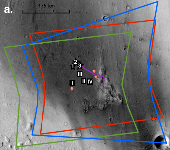
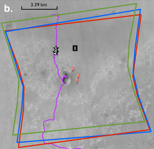
Figure 2: a. Image from Context camera (CTX) of the Spirit landing site at Gusev Crater with the rover path across the plain up to the Columbia hill in purple. The footprint of each selected CRISM observations (only the nadir image) is represented here (blue: FRT3192, green: FRT8CE1 and red: FRTCDA5). Full black stars point to the locations of the photometric measurements in the Gusev plains (1. Landing Site, 2. Bonneville Rim, 3. NW of Missoula) taken by instrument onboard Spirit (Johnson et al., 2006a). Full black squares represent the four ROIs that have been selected for our photometric study (ROI from I to IV). b. Image from CTX camera of the Opportunity landing site at Meridiani Planum with the rover path in purple. The footprint of each selected CRISM observations (only the nadir image) is represented here (blue: FRT95B8, green: FRT334D and red: FRTB6B5). Full black stars represent the locations of photometric measurements (1. South of Voyager, 2. Purgatory region) taken by Pancam instrument onboard Opportunity (Johnson et al., 2006b). Full black squares represent the selected ROI for our photometric study (ROI I).

2.3.2 Direct surface model: Hapke’s photometric model

Models describing the photometry of discrete granular media have been proposed to express the surface bidirectional reflectance using semi-empirical analytical approaches (e.g., Hapke, 1981a, b, 1984, 1986, 1993, 2002) and numerical approaches (e.g., Cheng and Domingue, 2000; Douté and Schmitt, 1998; Mishchenko et al., 1999).

Hapke’s modeling (Hapke, 1993) is widely used in the planetary community due to the simplicity of its expression and due to the fact that it introduces photometric parameters claimed to have physical relevance. Previous Martian photometric studies have been conducted based on orbital HRSC measurements (Jehl et al., 2008) and based on the analysis of in situ MER measurements (Johnson et al., 2006a, b) using the Hapke’s 1993 version model (Hapke, 1993). For this study, since we use the in situ investigation as “ground truth” in order to validate the MARS-ReCO approach, we have to use Hapke’s 1993 version model.

More recent Hapke models (Hapke, 2002, 2008) are available improving the original formulation (Hapke, 1981a, 1993) and can be used for future photometric studies. First, the model (Hapke, 2002) includes: (1) a more accurate analytic approximation for isotropic scatterers, (2) a better estimation of the bidirectional reflectance when the scatterers are anisotropic, and (3) the incorporation of coherent backscattering. Second, the model (Hapke, 2008) overcomes the limitations of the original model in order to predict porosity dependence of the bidirectional reflectance, in case of a particulate medium such as a planetary regolith. For that purpose the treatment of light propagating through the particle spacing.

Following Johnson et al. (2006a, b)’s works and for the sake of the comparison coherence we use the expression of Hapke (1993) as follows:

$$r\left(\theta_{0},\theta,g\right)=\frac{\omega}{4\pi}\,\frac{\mu_{0e}}{\left(\mu_{0e}+\mu_{e}\right)}\,\left\{\left[1+B(g)\right]P(g)+H(\mu_{0e})H(\mu_{e})-1\right\}S(\theta_{0},\theta,g),$$ (1)

• Geometry $\theta_{0}$, $\theta$, and $g$: The incidence, emergence and phase angles, respectively. .

• Single scattering albedo $\omega$: Factor $\omega$ ($0\leq\omega\leq 1$) depends on wavelength and represents the fraction of scattered light to incident light by a single particle (Chandrasekhar, 1960).

• Particle scattering phase function $P(g)$: Function $P(g)$ characterizes the angular distribution of an average particle. The empirical 2-term Henyey-Greenstein function (hereafter referred to as HG2) is used commonly for studying planetary surfaces (e.g., Cord et al., 2003; Hartman and Domingue, 1998; Jehl et al., 2008; Johnson et al., 2006a, b; Souchon et al., 2011). It reads:

  $$P(g)=\left(1-c\right)\,\frac{1-b^{2}}{\left(1+2b\cos\left(g\right)+b^{2}\right)^{3/2}}+c\,\frac{1-b^{2}}{\left(1-2b\cos\left(g\right)+b^{2}\right)^{3/2}}$$ (2)

  where the asymmetric parameter $b$ ($0\leq b\leq 1$) characterizes the anisotropy of the scattering lobe (from $b=0$, which corresponds to the isotropic case, to $b=1$, which corresponds to a particle which diffuses light in a single direction). The backscattering fraction $c$ ($0\leq c\leq 1$) characterizes the main direction of the diffusion ($c<0.5$ corresponding to forward scattering and $c>0.5$ corresponding to backward scattering).

• Multiple scattering function $H(x)$: The exact values of the $H$ function for isotropic scatterers was given by Chandrasekhar (1960). For consistency we use the approximation of isotropic scattering named H93 in the following (Hapke, 1993) as was done for the estimation of the surface photometric parameters by Johnson et al. (2006a, b). The H93 differs by a relative error on $H$ lower than 1% and a relative error on the bidirectional reflectance of a regolith lower than 2% (Cheng and Domingue, 2000). Defining $y=(1-\omega^{1/2}$, the multiple scattering function becomes:

  $$H(x)=\left\{1-\left[1-y\right]x\left[\left(\frac{1-y}{1+y}\right)+\left(1-\frac{1}{2}\left(\frac{1-y}{1+y}\right)-x\left(\frac{1-y}{1+y}\right)\right)\ln\left(\frac{1+x}{x}\right)\right]\right\}^{-1}$$ (3)

• Shadow Hiding Opposition Effect (SHOE) and Coherent Backscatter Opposition Effect (CBOE): $B(g)$ is a function designed to model the sharp increase of brightness around the zero phase angle often observed in the case of particulate media, the so-called opposition effect. The $B(g)$ function is given by Hapke (1993) as follows:

  $$B(g)=\frac{B_{0}}{1+\frac{1}{h}\tan\left(\frac{g}{2}\right)}.$$ (4)

  Parameters $h$ and $B_{0}$ are respectively the angular width and the amplitude of the opposition effect. Factor $h$ (ranging from 0 to 1) is physically related to compaction and particle size distribution and $B_{0}$ (ranging from $0$ to $1$) is an empirical parameter which is related to the particle transparency (Hapke, 1993). It is important to mention that the Ross-Thick Li-Sparse (RTLS) model for the surface reflectivity employed by MARS-ReCO (Ceamanos et al., 2013) is able to describe a backscattering lobe by means of its geometrical kernel. Nevertheless its angular width is more characteristic of photometric effects linked with shadows cast by macroscopic roughness than those occurring at the grain scale such as the SHOE and the CBOE (Lucht et al., 2000). Furthermore, the radiative transfer algorithm that is used to calculate the atmospheric quantities at the core of the MARS-ReCO procedure cannot propagate properly through the atmosphere the narrow backscattering lobes of the SHOE and CBOE. Finally, CRISM orbital measurements never reach the small phase angle domain ($\lesssim 5\text{\textdegree}$) where the previous phenomena are expressed. Consequently, MARS-ReCO is never in the position of retrieving accurate values for $B_{0}$ and $h$.

• Macroscopic roughness factor $S$: We note that planetary regoliths present roughness driven by grain clusters to the pixel scale. In the Hapke’s surface model this phenomena is described by a Gaussian distribution of slopes at a single spatial scale under the pixel size which is not explicitly given. The mean slope angle $\bar{\theta}$ is the only required parameter (Hapke, 1993). Surface roughness involves several radiative phenomena: (i) multiple reflection of light between facets, (ii) shadows depending on the geometry, (iii) bias on the incidence and emergence angles, and (iv) increase of the multiple scattering component. In order to quantify their influence on the bidirectional reflectance, Hapke’s model introduces a simple multiplicative factor $S$ depending on $\mu_{0e}$ and $\mu_{e}$ whose expressions are given in Hapke (1993).

2.3.3 Bayesian inversion of the surface model

The “inverse problem” consists in estimating the model parameters that best explain the observations. Unfortunately, inverse problems do not have a unique solution if the direct model is non-linear, as does the Hapke’s model. Tarantola and Valette (1982) proposed to solve inverse problems in a general non-linear case based on the concept of the state of information which is characterized by a Probability Density Function (PDF). The PDF is defined over both the parameter space and the observed space. The formalism of a PDF is used to define the initial state of information (i.e., a priori knowledge on the parameters, the uncertainties on the observation and on the model). To infer the solution, the Bayes’ theorem is applied. Key points concerning the bayesian inversion concept and framework assumptions are presented in the following:

• Data, model parameters and theoretical relationship: The direct model consists of computing the simulated data $d$, from model parameters $m$:

  $$d=F(m)$$ (5)

• Prior information on the model: The prior information on model parameters $\rho_{m}(m)$ in the parameter space $(M)$ is independent with the data and corresponds to the state of null information. For the Hapke model parameters $\omega$, $b$, $c$, $\bar{\theta}$, $B_{0}$ and $h$, we consider a uniform PDF, different from zero on an interval that insures their physical relevance (between $0$ and $1$ for $\omega$, $b$, $c$, $B_{0}$ and $h$ and between $0{{}^{\circ}}$ and $90{{}^{\circ}}$ for $\bar{\theta}$). Outside the intervals, the PDF is null, avoiding unphysical solution to appear. As discussed in Subsection 2.3.2 in real planetary situations, the SHOE and the CBOE phenomena are only expressed for phase angles $g$ $\lesssim 5\text{\textdegree}$ out of the range encompassed by typical CRISM observations ($g$ $\gtrsim 30\text{\textdegree}$). Thus a priori, neglecting both phenomena should not influence the retrieval of the other parameters . However following Souchon et al. (2011), the model can still be profitably inverted on the data by keeping parameters $B_{0}$ and $h$ since they will compensate for discrepancies between the model and the measurements in some situations. Consequently, in the present work, we first chose to invert the parameters $B_{0}$ and $h$ to systematically control if they are constrained or not by the CRISM data set. However in a second phase we also tested the inversion by setting $B_{0}$ and $h$ to zero and no change was observed on the determination of the other parameters ($\omega$, $\bar{\theta}$, $b$, $c$).

• Prior information on the data: The prior information on data $\rho_{d}(d)$ in the observation space $(D)$ is assumed to be a Gaussian PDF according to the MARS-ReCO formalism and retrieval strategy. Note that the error $\sigma$ on a CRISM measurement at one geometry is assumed to be independent on the state of the surface and on the other geometries (i.e., the PDF has a diagonal covariance matrix with elements $\sigma_{1}^{2},\ldots,\sigma_{N_{g}}^{2}$, where $N_{g}$ is the number of available geometries, up to 11). At 750 nm, the signal to noise ratio was estimated before launch to be equal to 450 (Murchie et al., 2007) but due to additional artifacts such as spikes, and calibration issues (Seelos et al., 2011) we evaluated the uncertainty $\sigma$ of the reflectance measurement ($\rho$) at each geometry $j$ to be of the order of $\sigma_{j}=(1/50)\times\rho_{j}$ where $j$=1,…,$N_{g}$ and $\rho_{j}$ is the CRISM dataset at the $j^{th}$ angular configuration (Ceamanos et al., 2013). Moreover, MARS-ReCO takes into account the uncertainty of the AOT input. Figure 3 presents a typical TOA photometric curve collected by the CRISM instrument (green plus) and the bidirectional reflectance curve produced by the MARS-ReCO algorithm (red crosses). For each geometry the bidirectional reflectance value is accompanied by its $1\sigma$ uncertainty. Those means and root mean square errors are used to build $\rho_{d}(d)$ that serves as an input PDF of the Bayesian inversion.

• Posterior probability density function and resolution of inverse problems: Inversion problems correspond to the particular case where information from the data space $(D)$ is translated into the model space $(M)$. The posterior PDF in the model space $\sigma_{M}(m)$ as defined by Tarantola and Valette (1982) reads

  $$\sigma_{M}(m)=k\,\rho_{M}(m)\,L(m),$$ (6)

  where $k$ is a constant and $L(m)$ is the likelihood function

  $$L(m)=\int_{D}\partial d\,\frac{\rho_{D}(d)\,\theta(d\mid m)}{\mu_{D}(d)},$$ (7)

  where $\theta(d\mid m)$ is the theoretical relationship of the PDF for $d$ given $m$, and $\mu_{D}(d)$ is null information PDF for the data $d$. The solution of the general inverse problem is given by the PDF $\sigma_{M}(m)$ from which any information on the model parameter can be obtained such as mean values, uncertainty bars, etc . Please refer to Tarantola and Valette (1982) for more detail.

• Sampling of solutions to inverse problems: In our case, the relationship between model parameters and observed data through Hapke’s modeling is non-linear. While it is not possible to describe the posterior PDF analytically, it can be sampled using a Monte Carlo approach using a Markov chain (Mosegaard and Tarantola, 1995). After a sufficient number of steps, the state of the chain corresponds to the desired distribution. According our tests, the best trade-off between computation time and accuracy is a burn-in phase (phase in which the Markov chain approaches a stationary state after a certain number of runs) of 500 steps. The next 500 iterations are used to estimate the posterior PDF allowing the determination of the mean and standard deviation of each parameter. Note that a posteriori PDF of a retrieved parameter is not necessarily a gaussian distribution but can be a square function or multi-modal as seen in Figures 4 and 6. To describe the results of each parameter, we choose to compute the mean of the posterior PDF. To describe the uncertainties, we choose to compute the standard deviation. We warn the reader because sometimes these estimators can be inappropriate to describe the PDF. In the following graphs, $2\sigma$ error bars are plotted to describe more accurately the PDFs.

• Root Mean Square residual $RMS$: In order to estimate the difference between the fit and the observed bidirectional reflectance, the Root Mean Square residual (noted $RMS$) is given for each Bayesian inversion as follows:

  $$RMS=\sqrt{\frac{\sum_{N_{g}}\left(\rho_{obs}-\rho_{mod}\right)^{2}}{N_{g}}}$$ (8)

  where $N$ is the available geometric configurations, $\rho_{obs}$ the CRISM bidirectional reflectance corrected for atmosphere and $\rho_{mod}$ the modeled bidirectional reflectance taken as the mean of the 500 iterations used to estimate the posterior PDF.

• Non-uniformity criterion $k$: Photometric parameters $m$ are constrained if their marginal posterior PDF differs from the prior state of information (i.e., a null information taken as a uniform distribution, in our case). In order to distinguish if a given parameter has a solution we perform a statistical test leading to a non-uniformity criterion $k$ (see Appendix A). For $k>0.5$, the marginal posterior PDF is considered to be non-uniform and thus we consider that the mean and standard deviation of the PDF satisfactorily describe the solution(s).

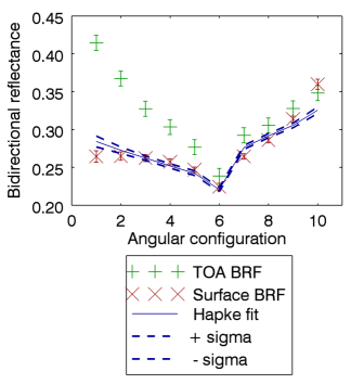
Figure 3: Reflectance values (in BRF units) corresponding to the photometric curve of the ROI I from FRT3192 observation composed of ten angular configurations at the TOA (green plus), and at the surface after the correction for atmospheric contribution carried out by MARS-ReCO (red crosses). In both cases the $1\sigma$ uncertainty is expressed as a function of angular configuration (the eleven geometric views of one CRISM EPF scans from 1st to 5th corresponds to the inbound direction, 6th is the central scan and from 7th to 11th are related to the outbound direction). The latter data are used in the Bayesian inversion. The blue solid and dashed lines represent the Hapke’s best fit and their $1\sigma$ uncertainties, respectively.

3 Analysis of retrieved photometric parameters

As mentioned in Subsection 2.1.2, we selected three CRISM targeted observations from Gusev Crater and from Meridiani Planum (cf. Table 1). All observations were individually corrected for aerosols using MARS-ReCO, knowing the respective AOT values (cf. Table 1). Based on the corrected bidirectional reflectance, we use the proposed methodology described in Subsection 2.3.3 to estimate the photometric parameters of the materials encompassed by four ROIs in the case of Gusev Crater (ROI I to ROI IV) and by one ROI in the case of Meridiani Planum (ROI I).

For each ROI, we determine the surface photometric parameters at 750 nm from (i) a single CRISM FRT observation or (ii) a combination of all selected FRT observations (i.e., FRT3192, FRT8CE1 and FRTCDA5 in the case of Gusev Crater, and FRT95B8, FRT334D and FRTB6B5 in the case of Meridiani Planum). Remember that the chosen targeted observations are complementary in terms of phase angle range (cf. Table 1).

For each parameter of the photometric Hapke’s model (i.e., $\omega$, $b$, $c$, $\bar{\theta}$, $B_{0}$ and $h$) we determine its mean value and standard deviation by running the proposed Bayesian inversion procedure. The non-uniform criterion noted $k$ is conjointly computed and detailed in Tables 3 and 4 for Gusev Crater and Table 5 for Meridiani Planum. In the following, we have two criteria that help us estimate the existence and the quality of a solution. On the one hand, the non-uniform criteria $k$ allows us to reject posterior PDF’s that do not carry a solution. On the other hand, the standard deviation allows us to quantify to which extent a given parameter is constrained by the current solution.

3.1 Results on Gusev Crater

Table 3: Retrieved Hapke’s parameters ($\omega$, $b$, $c$, $\bar{\theta}$ in degree, $B_{0}$, $h$) and their standard deviation in parentheses (the underconstrained parameters are indicated by "(-)") corresponding to the ROI I and II from CRISM measurement at 750 nm using our Bayesian inversion as well as the non-uniform criterion $k$ (second line of each entry) after MARS-ReCO. This analysis is done for each CRISM FRT observation (i.e., FRT3192, FRT8CE1 and FRTCDA5) or for the combination of the three observations after correction for the atmospheric effects by MARS-ReCO. The standard deviation $\sigma_{\rho}$ (in BRF units) is a parameter provided by MARS-ReCO estimating the quality of the retrieved surface bidirectional reflectance. The absolute quadratic residual of the fit $RMS$ (in BRF units) evaluates the deviation of the fit from observed bidirectional reflectance. ($nb$: number of angular configurations $g$: phase angle range in degree)

FRT	Lat.	Lon.	AOT	$\sigma_{\rho}$	$\omega$	$b$	$c$	$\bar{\theta}$	$B_{0}$	$h$	$nb$	$g$
	(°N)	(°E)		$RMS$	$k$	$k$	$k$	$k$	$k$	$k$
3192	-14.603	175.478	0.33$\pm$0.04	0.01	0.68 (0.06)	0.17 (0.20)	0.62 (0.20)	11.62 (3.98)	0.52 (-)	0.52 (-)	10	$\sim$56-112
				0.01	1.00	1.92	0.96	1.00	0.24	0.12
8CE1	-14.606	175.478	0.98$\pm$0.15	0.03	0.77 (0.07)	0.30 (0.28)	0.42 (0.27)	17.23 (9.64)	0.47 (-)	0.50 (-)	9	$\sim$37-79
				0.01	1.00	1.47	0.60	0.98	0.20	0.12
CDA5	-14.604	175.481	0.32$\pm$0.04	0.01	0.78 (0.08)	0.44 (0.32)	0.54 (0.23)	16.71 (4.64)	0.51 (-)	0.52 (-)	8	$\sim$46-107
				0.00	0.99	0.91	0.70	1.00	0.05	0.30
ROI I - 3 FRTs	-	-	-	-	0.71 (0.05)	0.22 (0.18)	0.54 (0.18)	15.78 (2.65)	0.49 (-)	0.54 (-)	27	$\sim$37-112
				0.01	1.00	1.45	0.95	1.00	0.28	0.23

FRT	Lat.	Lon.	AOT	$\sigma_{\rho}$	$\omega$	$b$	$c$	$\bar{\theta}$	$B_{0}$	$h$	$nb$	$g$
	(°N)	(°E)		$RMS$	$k$	$k$	$k$	$k$	$k$	$k$
3192	-14.599	175.499	0.33$\pm$0.04	0.01	0.72 (0.08)	0.29 (0.31)	0.59 (0.20)	12.32 (5.26)	0.52 (-)	0.52 (-)	9	$\sim$55-112
				0.01	1.00	1.69	0.92	1.00	0.23	0.16
8CE1	-14.603	175.500	0.98$\pm$0.15	0.03	0.76 (0.08)	0.34 (0.29)	0.44 (-)	17.58 (9.91)	0.48 (-)	0.48 (-)	7	$\sim$36-90
				0.02	0.99	1.42	0.41	0.98	0.08	0.09
CDA5	-14.602	175.498	0.32$\pm$0.04	0.01	0.74 (0.07)	0.37 (0.28)	0.65 (0.20)	14.62 (4.97)	0.53 (-)	0.51 (-)	8	$\sim$46-107
				0.01	1.00	1.06	0.81	1.00	0.14	0.10
ROI II - 3 FRTs	-	-	-	-	0.72 (0.05)	0.27 (0.15)	0.56 (0.16)	15.62 (2.43)	0.49 (-)	0.52 (-)	24	$\sim$36-112
				0.01	1.00	1.18	0.99	1.00	0.05	0.23

Table 4: Same as Table 3 but for the ROI III and ROI IV

FRT	Lat.	Lon.	AOT	$\sigma_{\rho}$	$\omega$	$b$	$c$	$\bar{\theta}$	$B_{0}$	$h$	$nb$	$g$
	(°N)	(°E)		$RMS$	$k$	$k$	$k$	$k$	$k$	$k$
3192	-14.593	175.496	0.33$\pm$0.04	0.01	0.72 (0.08)	0.32 (0.29)	0.58 (0.20)	10.53 (5.81)	0.50 (-)	0.50 (-)	7	$\sim$56-108
				0.01	1.00	1.12	0.94	1.00	0.15	0.10
8CE1	-14.596	175.494	0.98$\pm$0.15	0.03	0.77 (0.09)	0.35 (0.29)	0.44 (-)	19.13 (10.52)	0.49 (-)	0.51 (-)	7	$\sim$37-84
				0.01	0.99	1.36	0.39	0.98	0.02	0.06
CDA5	-14.594	175.497	0.32$\pm$0.04	0.01	0.72 (0.07)	0.26 (0.25)	0.65 (0.20)	14.21 (5.59)	0.51 (-)	0.54 (-)	7	$\sim$46-106
				0.01	1.00	1.67	0.85	1.00	0.15	0.24
ROI III - 3 FRTs	-	-	-	-	0.69 (0.04)	0.19 (0.14)	0.66 (0.18)	13.96 (4.40)	0.50 (-)	0.53 (-)	21	$\sim$37-108
				0.01	1.00	1.43	0.87	1.00	0.08	0.11

FRT	Lat.	Lon.	AOT	$\sigma_{\rho}$	$\omega$	$b$	$c$	$\bar{\theta}$	$B_{0}$	$h$	$nb$	$g$
	(°N)	(°E)		$RMS$	$k$	$k$	$k$	$k$	$k$	$k$
3192	-14.600	175.507	0.33$\pm$0.04	0.01	0.68 (0.06)	0.17 (0.21)	0.61 (0.22)	11.74 (4.43)	0.53 (-)	0.56 (-)	9	$\sim$56-112
				0.01	1.00	1.80	0.97	1.00	0.28	0.39
8CE1	-14.602	175.508	0.98$\pm$0.15	0.04	0.78 (0.09)	0.38 (0.29)	0.47 (-)	20.40 (11.41)	0.51 (-)	0.50 (-)	6	$\sim$41-84
				0.01	0.99	0.80	0.24	0.97	0.22	0.12
CDA5	-14.600	175.509	0.32$\pm$0.04	0.01	0.74 (0.07)	0.35 (0.27)	0.65 (0.20)	14.55 (5.48)	0.51 (-)	0.50 (-)	8	$\sim$46-107
				0.01	1.00	1.10	0.79	1.00	0.14	0.09
ROI IV - 3 FRTs	-	-	-	-	0.79 (0.07)	0.59 (0.27)	0.56 (0.16)	10.88 (5.11)	0.50 (-)	0.48 (-)	23	$\sim$41-112
				0.01	1.00	0.53	0.97	1.00	0.09	0.05

The quality of the surface bidirectional reflectance estimated by MARS-ReCO is given by the standard deviation $\sigma_{\rho}$. This quality parameter is available for each ROI of each CRISM targeted observation of the present study (cf. Tables 3 and 4). The highest $\sigma_{\rho}$ value is observed for FRT8CE1 which can be explained by a wrong AOT estimation (highest AOT value) in this case (i.e., FRT8CE1: $\sigma_{\rho}$ = 0.03-0.04 for AOT = 0.98). The positive correlation of this uncertainty and the AOT is also observed in the sensitivity study led by Ceamanos et al. (2013). Indeed the error computed for synthetic reference data mimicking the photometric properties of the planet Mars increases with AOT (i.e., for AOT = 1, $\sigma_{\rho}\sim$ 0.05 and error is $\sim$10% while for AOT = 1.5, $\sigma_{\rho}\sim$ 0.10 and error is $\sim$20%, see Ceamanos et al. (2013) for more detail).

Tables 3 and 4 present results regarding the Hapke’s model parameters for the different ROIs of Gusev Crater.

The goodness of fit is estimated through the absolute quadratic residual $RMS$ value (cf. Tables 3 and 4). For all Bayesian inversions, the estimates are less than 0.02 which mean that the inversions are deemed satisfactory.

Figure 4 represents the PDF of each parameter considering the inversion of a single FRT observation as well as the inversion of the three combined observations. According to results, a solution exists for parameters $\omega$, $b$, $c$ and $\bar{\theta}$ (because the PDF is non-uniform) whereas no solution exists for parameters $B_{0}$ and $h$ (uniform PDF). Several conclusions can be drawn when using a single targeted observation:

• Solutions exist for parameter $\omega$ in all cases ($k\sim 1$). The standard deviation shows that the single scattering albedo is the most constrained parameter (i.e., 0.06 < $\sigma$ < 0.09). Examples of posteriori PDFs are plotted in Figures 4 and 9.

• Although solutions exist for parameter $b$ in all cases ($k$ >> 0.5), the standard deviation shows that it is poorly constrained (i.e., 0.25 < $\sigma$ < 0.32) except for the ROI I and ROI IV using the CRISM observation FRT3192. This discrepancy can be explained by the higher number of available geometric configurations, respectively 10 and 9. Examples of posteriori PDFs are plotted in Figures 4 and 10.

• We find meaningful values for parameter $c$ only when we use FRT3192 or FRTCDA5 ($k$ > 0.5). The standard deviation is relatively low (i.e., 0.20 < $\sigma$ < 0.23) in this case. In the case of FRT8CE1, no solution is found for parameter $c$ ($k$ < 0.5) for ROI II, III and IV. For the ROI I, however, a solution exists but it is poorly constrained (i.e., $\sigma$ = 0.27). Examples of posteriori PDFs are plotted in Figures 4 and 10.

• While parameter $\bar{\theta}$ has a solution in all cases ($k\sim 1$), we distinguish two types of results: (i) using FRT3192 or FRTCDA5, we note that the standard deviation is relatively low (i.e., 3.98 < $\sigma$ < 5.81), and (ii) using FRT8CE1, the standard deviation is relatively high (i.e., 9.64 < $\sigma$ < 20.40) .Examples of posteriori PDFs are plotted in Figures 4 and 11.

• No solutions are found for parameters $B_{0}$ and $h$ in any case ($k$ << 0.5). As mentioned in Subsection 2.3.2, nor the phase domain covered by the CRISM observations nor the capabilities of MARS-ReCO allow to constrain the opposition effect (Ceamanos et al., 2013). Consequently, accurate values for $B_{0}$ and $h$ cannot be retrieved and no physical interpretation can be done in this case. Examples of posteriori PDFs are plotted in Figure 4.

Regarding the processing of a single CRISM observation, we note that parameters $c$ and $\bar{\theta}$ are, respectively, non-constrained and poorly constrained only when treating data from FRT8CE1. The reason to explain such a difference may be that the available maximum phase angle range is less than 90° for FRT8CE1. Indeed, Helfenstein (1988) underlined the necessity to have observations which extend from small phase angles out to phase angles above 90° for an accurate determination of the photometric roughness. By contrast, the phase angle range expands by more than 100° for the other observations (cf. Table 1). We note that parameter $b$ is poorly constrained when treating data from all available observations. This result may be explained again by the available phase angle range (cf. Table 1). In conclusion, the presented study clearly demonstrates that the existence and quality of a solution for parameters $b$, $c$ and $\bar{\theta}$ is dependent on the available phase angle range. The bidirectional reflectance curve from a single CRISM observation does not contain enough phase angle information.

By contrast, the combination of three targeted observations provides improved constrains on all Hapke’s parameters except for $B_{0}$ and $h$. Indeed, the standard deviation of each estimated parameter is lower than those obtained when using only a single targeted observation. We note that for ROI IV, the Hapke’s parameters are less constrained than for the other ROIs, especially for parameter $b$ for which no solutions were found. This result can be explained by the limitation in the bidirectional sampling. In fact, we can note in Figure 5 which represents the north projection of geometric conditions for the four selected ROIs that the ROI IV misses a near nadir geometry from the observation FRT8CE1. The latter shows a more different incidence angles (nearly 40°) than the two other CRISM FRT observations (nearly 60°) (see also Table 1) thus explaining that the parameters are less constrained for ROI IV than the other ROI.

To conclude, the quality of these results show the benefits of combining several targeted observations in constraining photometric parameters.

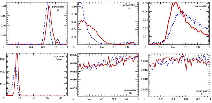
Figure 4: The PDF of each of the six physical parameters retrieved for ROI I. Two cases are considered: the inversion of a single CRISM FRT observation (i.e., FRT3192 in blue line) and the inversion of three combined CRISM FRT observations (in red line).

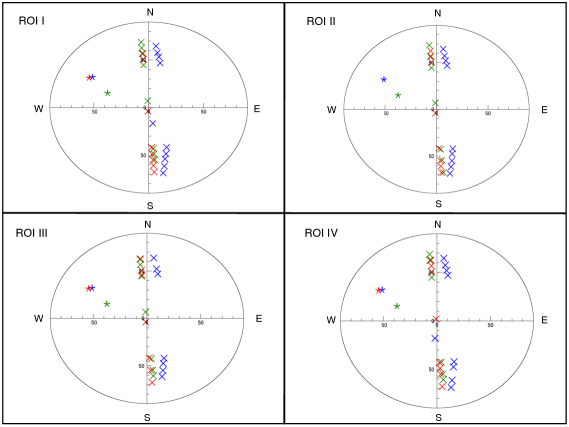
Figure 5: North projection of geometric conditions (stars: incidence rays and crosses: emergence directions) of the four selected ROIs for the Gusev Crater study (blue: FRT3192, green: FRT8CE1 and red: FRTCDA5).

3.2 Results on Meridiani Planum

Table 5: Same as Table 3 but for Meridiani Planum with CRISM FRT observations FRT95B8, FRT334D and FRTB6B5.

FRT	Lat.	Lon.	AOT	$\sigma_{\rho}$	$\omega$	$b$	$c$	$\bar{\theta}$	$B_{0}$	$h$	$nb$	$g$
	(°N)	(°E)		$RMS$	$k$	$k$	$k$	$k$	$k$	$k$
95B8	-2.000	-5.484	0.56$\pm$0.09	0.02	0.72 (0.09)	0.34 (0.30)	0.42 (-)	17.32( 10.33)	0.48 (-)	0.50 (-)	5	$\sim$41-86
				0.01	0.99	1.40	0.44	0.98	0.12	0.16
334D	-2.001	-5.482	0.35$\pm$0.04	0.01	0.67 (0.09)	0.38 (0.32)	0.49 (0.25)	16.65 (7.82)	0.49 (-)	0.48 (-)	5	$\sim$50-98
				0.01	0.99	1.16	0.61	1.00	0.18	0.16
B6B5	-2.004	-5.482	0.35$\pm$0.04	0.01	0.65 (0.07)	0.19 (0.20)	0.52 (-)	18.09 (5.82)	0.50 (-)	0.50 (-)	6	$\sim$41-106
				0.01	1.00	2.06	0.41	1.00	0.12	0.14
ROI I - 3 FRTs	-	-	-	-	0.68 (0.08)	0.36 (0.26)	0.41 (0.21)	18.37 (5.20)	0.51 (-)	0.52 (-)	16	$\sim$41-106
				0.02	0.99	0.82	0.95	1.00	0.15	0.24

Similar to the photometric study on the Gusev Crater, the standard deviation $\sigma_{\rho}$ determined by MARS-ReCO is given for each CRISM observation and the ROI I used for the present study (cf. Table 5). Note that $\sigma_{\rho}$ values are acceptable (0.01 < $\sigma_{\rho}$ < 0.02) meaning that estimated surface bidirectional reflectance are accurate.

Table 5 presents the results obtained on Meridiani Planum. Similar to Gusev Crater study, Figure 6 shows that a solution exists for the parameters $\omega$, $b$, $c$ and $\bar{\theta}$ (i.e., non-uniform PDF) when a single CRISM FRT and in the case of three combined observations, except for parameters $B_{0}$ and $h$.

The goodness of fit is estimated through the absolute quadratic residual $RMS_{abs}$ value (cf. Table 5). For all bayesian inversions, the estimates are less than 0.02 which mean that the inversions are deemed satisfactory.

We note that for the parameter $\omega$, two maximum are visible at nearly 0.6 and 0.8. In order to understand the origin of the bimodal distribution for the parameter $\omega$ in this case, the reflectance of typical Martian material was generated by using realistic photometric properties determined by the Pancam instrument aboard the MER Opportunity site in Meridiani Planum (i) at the same geometric configurations as the FRT95B8 observations, and (ii) at the same combined geometric configurations when merging the three selected observations. In both cases, the posterior PDF for the parameter $\omega$ shows a bimodal distribution. If the geometric sampling is broader (i.e., with varied incidence, emergence and phase angles), the posterior PDF of the parameter $\omega$ becomes a gaussian with a single peak. The presence of two possible solutions is the consequence of the limitation of a sufficient geometric diversity in our selection of CRISM observations for the Meridiani Planum study to constrain the parameter $\omega$, which is otherwise the best-constrained parameter in photometric modeling.

Several conclusions can be drawn when using a single CRISM targeted observation:

• Solutions exist for parameter $\omega$ in all cases ($k\sim 1$). The standard deviation shows that the single scattering albedo is the most constrained parameter (i.e., 0.07 < $\sigma$ < 0.15). Examples of posteriori PDFs are plotted in Figures 6 and 13.

• We find meaningful values for parameter $b$ only when for FRT95B8 or FRT334D or FRTB6B5 ($k$ > 0.5). Albeit the standard deviation is relatively high for FRT95B8 or FRT334D (i.e., 0.30 < $\sigma$ < 0.32), the standard deviation becomes relatively low for FRTB6B5 (i.e., $\sigma$ = 0.20). Examples of posteriori PDFs are plotted in Figures 6 and 14.

• Solutions only exist for parameter $c$ when using FRT334D ($k$ > 0.5). However, the standard deviation is relatively high ($\sigma$ = 0.25). Examples of posteriori PDFs are plotted in Figures 6 and 14.

• While parameter $\bar{\theta}$ has a solution in all cases ($k\sim 1$), we distinguish two types of results: (i) using FRT334D or FRTB6B5, we note that the standard deviation is relatively low (i.e., 5.82 < $\sigma$ <7.82) and (ii) the standard deviation is relatively high (i.e., $\sigma$ = 10.33) when using FRT95B8. Examples of posteriori PDFs are plotted in Figures 6 and 15.

• Similar to the Gusev study, no solution is found for parameters $B0$ and $h$ in any case ($k$ >> 0.5). Examples of posteriori PDFs are plotted in Figure 6.

Dealing with single observations, we note that parameter $\bar{\theta}$ is poorly constrained when treating data from FRT95B8 and FRT334D whereas it is highly constrained when using FRTB6B5 which can be explained by a maximum phase angle below 90° in case of FRT95B8 and FRT334D (cf. Table 1). Helfenstein (1988) underlined the necessity to have observations which extend from small phase angles out to phase angles above 90° for an accurate determination of the photometric roughness. Note that parameter $b$ and $c$ are non-constrained or poorly constrained even through solutions exist in all cases. This outcome can be explained by a worse quality of the Meridiani Planum bidirectional reflectance sampling. Indeed, we note in Figure 7 which represents the north projection of geometric conditions of each selected CRISM FRT observations that the three selected CRISM FRT (i) miss near nadir geometries (close to emergence equal 0) and (ii) present lower number of available angular configurations compared to Gusev Crater work (lower than 6).

We then improve the bidirectional reflectance sampling by combining the three selected targeted observations. We observe that parameters $\omega$, $b$, $\bar{\theta}$ become significantly more constrained. Indeed, the standard deviation of each estimated parameter is lower than those obtained when using only a single observation. However, the parameters are less constrained than those obtained for the Gusev Crater study, which can be explained by the lack of near nadir geometry for this case (cf. Figure 7).

Again, results underline the benefits of combining several observations.

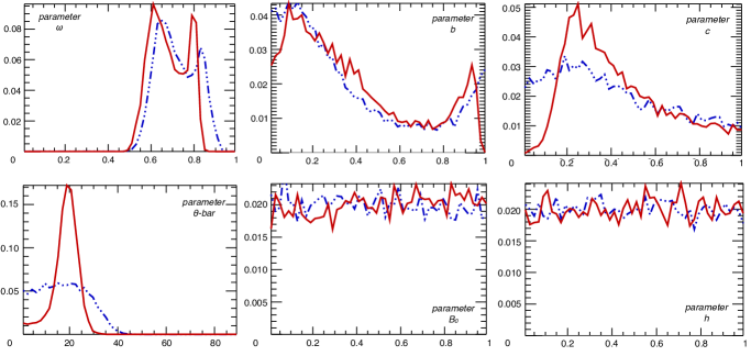
Figure 6: The PDF of each of the six physical parameters retrieved for ROI I of Meridiani Planum. Two cases are considered: the inversion of a single CRISM FRT observation (i.e., FRT95B8 in blue line) and the inversion of three combined CRISM FRT observations (in red line).

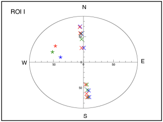
Figure 7: North projection of geometric conditions (stars: incidence directions and crosses: emergence directions) of the selected ROI for the Meridiani Planum study (blue: FRT95B8, green: FRT334D and red: FRTB6B5).

4 Validation

This section focuses on the validation of the estimated photometric parameters by comparing them to previous photometric studies based on experimental, in situ and orbital photometric studies. As the PDF of each parameter is not necessary a gaussian, the estimated mean and the standard deviation are not always representative of the entire distribution. Consequently for each parameter, we use the PDF built from the last 500 iterations of the Markov chain process (see 2.3.1) instead of the previous statistical estimators for the comparison to previous studies.

4.1 Validation of results from Gusev crater

4.1.1 Comparison to experimental measurements on artificial and natural samples

McGuire and Hapke (1995) studied the scattering properties of different isolated artificial particles which have different structure types (sphere/rough particles, clear/irregular shape particle, with/without internal scatterers, …). Their study showed that the Henyey-Greenstein function with two parameters, HG2 (backscattering fraction $c$ and asymmetric parameter $b$) provided the best description of their laboratory bidirectional reflectance measurements. In short, their study shows that smooth clear spheres exhibit greater forward scattering (low values of $c$) and narrower scattering lobes (high values of $b$) whereas particles characterized by their roughness or internal scatterers exhibit greater backward scattering (high values of $c$) and broader scattering lobe (low values of $b$). In a graph mapping the $b$ and $c$ parameter space, the results exhibit a “L-shape” from particles with high density of internal scatterers to smooth, clear, spherical particles. For their study, McGuire and Hapke (1995) used centimeter sized artificial particles which are larger than the light wavelength and far than typical constituents of the planetary regoliths. In order to examine the impact of particle size on the scattering phase function, Hartman and Domingue (1998) observed that there are no significant variations of the latter in McGuire and Hapke (1995) measurements when the particle size is similar to typical planetary regoliths particles. Hartman and Domingue (1998) concluded that McGuire and Hapke (1995) results could be considered to be representative of their respective particle structure types independent of particle size. However, recent experimental works have questioned the initial interpretation of the Hapke’s parameters. Indeed, the Hapke’s parameters seem to be more sensitive to the organization of the surface material (effects of close packing, micro-roughness) than to the optical properties depending on individual particles (Cord et al., 2003; Shepard and Helfenstein, 2007). Similarly, Souchon et al. (2011) measured for a comprehensive set of geometries the reflectance factor of natural granular surfaces composed of volcanic materials differing by their grain size (from the micron-scale to the millimeter-scale), shapes, surface aspect, and mineralogy (including glass and minerals). Thus the main novelty of Souchon et al. (2011)’s experimental study compared to McGuire and Hapke (1995)’s works is the determination of the parameters $b$ and $c$ for planetary analogs of basaltic granular surfaces and not isolated artificial particles. Souchon et al. (2011) compared the scattering parameters retrieved by inversion of Hapke’s model with results on artificial materials (McGuire and Hapke, 1995) and a similar trend was found, though with some variations and new insights. Granular surfaces even with a moderate proportion of isolated translucent monocrystals and/or fresh glass exhibit strongly forward scattering properties and a new part of the L-shape domain in the $b$ and $c$ parameter space is explored.

In Figure 8 that is given as an example of similar figures, the scattering parameters (i.e., backscattering fraction $c$ and asymmetric parameter $b$) of the ROI I from CRISM data (cf. Table 3) are plotted along with the scattering parameters obtained from laboratory measurements of artificial (McGuire and Hapke, 1995) and natural samples (Souchon et al., 2011). Results shows that parameters $b$ and $c$ retrieved from the inversion of combined CRISM FRT observations are consistent with the laboratory studies. The combination of three FRTs is necessary to constrain satisfactorily the $b$ and $c$ values with acceptable error bars. As it can be seen, surface materials of ROI I have high values of $c$ and low values of $b$, which indicate broad backscattering properties related to artificial materials composed of spheres with a moderate density of internal scatterers and close to irregular or round rough, opaque and solid natural particles (cf. Figure 8).

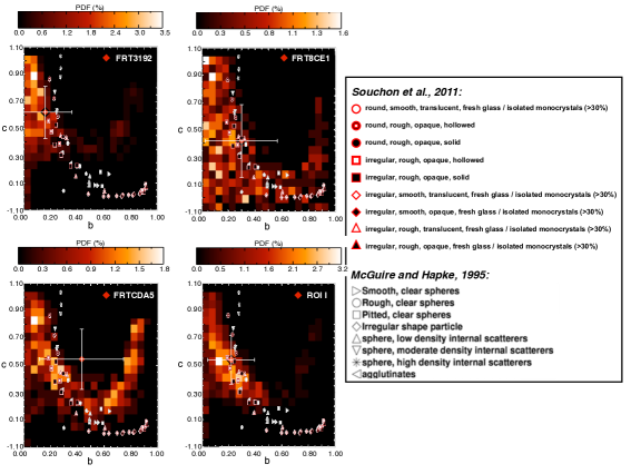
Figure 8: Probability density map of the asymmetric parameter $b$ (horizontal axis) versus the backscattering fraction $c$ (vertical axis) solutions retrieved at 750 nm estimated from the last 500 iterations of the Bayesian inversion for FRT3192, FRT8CE1 and FRTCDA5 observations and their combination (ROI I). The grid is divided into 24 (vertical) x 20 (horizontal) square bins. The coloring gives the probability corresponding to each bin. Means and 2$\sigma$ uncertainties (red rhombus) are plotted too. The inversion solutions are plotted against the experimental $b$ and $c$ values pertaining to artificial particules measured by McGuire and Hapke (1995) and to natural particles measured by Souchon et al. (2011).

4.1.2 Comparison to in situ measurements taken by Pancam/MER-Spirit

The Pancam instrument on-board MER-Spirit acquired several spectrophotometric observations along the rover’s traverse paths to determine the surface physical and chemical properties of rocks and soils encountered at the Gusev Crater. Johnson et al. (2006a) evaluated the parameters of Hapke’s photometric model (Hapke, 1993) using Equations 1, 2 and 3 from measured radiance for several identified units (i.e., “Gray” rocks, which are free of airfall-deposit dust or other coatings, ”Red” rocks, which have coating, and ”Soil” unit, corresponding to unconsolidated materials). The measured radiance at the ground was first corrected for diffuse sky illumination (Johnson et al., 2006a) and local surface facet orientations (Soderblom et al., 2004).

The difference of spatial resolution between CRISM and Pancam instruments must be considered prior to comparison. Indeed, a direct comparison between both sets of photometric parameters must be handled with care as Pancam provides local measurements (at a centimetric scale such as soils and rocks), whereas orbital instruments such as CRISM measure extended areas integrating different geologic units (at a pluri-decametric scale such as a landscape). In the latter case, measurements may be dominated by unconsolidated materials such as soils. As mentioned in Subsection 2.3.1, the four selected ROIs are chosen close to the MER-Spirit’s path. The retrieved photometric parameters for each ROI from the combination of three CRISM observations were compared to those extracted from three sequences taken by Pancam in the Gusev plains. These measurements are located near to the four ROIs in Landing site (Sol 013), Bonneville Rim (Sol 087-088) and Missoula (Sol 102-103) to the northwest side of Columbia Hill (cf. Figure 2) (Johnson et al., 2006a). In this case the combination of three CRISM observations were treated using the H93 version of the Hapke’s model in order to match the same model used in Johnson et al. (2006a). Pancam results are summarized in Table 6.

Table 6: Retrieved Hapke’s parameters and their standard deviation (underconstrained parameters are indicated by “(+,-)”) from the 2-term model for Sol 13, Sol 87-88 and Sol 102-103 and each of the three considered units (Gray Rock, Red Rock and Soil) at 753 nm (except for the parameter $c$ of Red Rock unit for Landing Site which corresponds to the 754 nm model results) from Pancam onboard Spirit (Johnson et al., 2006a)

Site	Unit	$\omega$	$\bar{\theta}$ (deg.)	$b$	$c$	Number	$g$ (deg.)
Landing Site	Bright Soil	0.75 (+0.01, -0.00)	2 (+, -)	0.243 (+0.020, -0.017)	0.625 (+0.012, -0.013)	21	$\sim$30-120
(Sol 013)	Gray Rock	0.83 (+0.01, -0.01)	7 (+3, -4)	0.931 (+0.045, -0.044)	0.065 (+0.058, -0.058)	66	$\sim$30-120
	Red Rock	0.79 (+0.03, -0.02)	20 (+3, -3)	0.187 (+0.026, -0.031)	0.720 (+0.084, -0.087)	68	$\sim$30-120
	Soil	0.76 (+0.01, -0.01)	15 (+2, -1)	0.262 (+0.010, -0.010)	0.715 (+0.029, - 0.032)	51	$\sim$30-120
Bonneville Rim	Gray rock	0.72 (+0.04, -0.04)	23 (+3, -4)	0.434 (+0.035, -0.037)	0.359 (+0.048, -0.050)	63	$\sim$25-120
(Sol 087-088)	Red rock	0.70 (+0.01, -0.01)	15 (+3, -3)	0.219 (+0.017, -0.020)	1.000 (+, -)	72	$\sim$25-120
	Soil	0.66 (+0.00, -0.00)	7 (+1, -1)	0.170 (+0.008, -0.008)	0.823 (+0.025, -0.024)	54	$\sim$25-120
NW of Missoula	Gray rock	0.70 (+0.02, -0.02)	13 (+2, -3)	0.406 (+0.018, -0.032)	0.206 (+0.019, -0.025)	225	$\sim$0-125
(Sol 102-103)	Red rock	0.83 (+0.02, -0.02)	19 (+1, -2)	0.450 (+0.023, -0.064)	0.255 (+0.032, -0.072)	141	$\sim$0-125
	Soil	0.69 (+0.01, -0.00)	11 (+1, -1)	0.241 (+0.011, -0.009)	0.478 (+0.036, -0.022)	132	$\sim$0-125

• Single scattering albedo: Figure 9 plots means and uncertainties as well as the PDF of single scattering albedo $\omega$ estimated for the four selected ROIs against values extracted for each unit defined by Johnson et al. (2006a) (i.e., Gray rocks, Red rocks and Soil) at the Landing site, Bonneville rim and NW of Missoula. The bimodality is identical to Meridiani ROI I (see subsection 3.2) and is the consequence of the lack of geometric diversity in the CRISM dataset. The estimated values of $\omega$ from CRISM are consistent with the Pancam outputs for the Soil unit.

  

  Figure 9: Mean and uncertainties of the single scattering albedo $\omega$ estimated from Pancam measurements at 753 nm for different geological units at Landing Site (Sol 013), Bonneville Rim (Sol 087-088) and NW of Missoula (Sol 102-103) (Johnson et al., 2006a) compared to those estimated from CRISM measurements at 750 nm (note that the error bar represents 2$\sigma$ uncertainties) derived from 2-term HG models. The PDFs of the parameter $\omega$ estimated from the last 500 iterations of the bayesian inversion are also represented on the left side. This is helpful when mean and uncertainties are not entirely representative of the PDF (such as the PDF of the parameter $\omega$ for the ROI IV which shows a bimodal distribution).

• Phase function: Figure 10 plots the asymmetric parameter $b$ versus the backscattering fraction $c$ solutions provided by the Bayesian inversion for each ROI in comparison to the photometric parameters obtained by Johnson et al. (2006a). In the case of Red Rock unit for Landing Site, the parameter $c$ is determined at 754 nm instead of usual 753 nm. Moreover, the parameter $c$ is not constrained at both wavelengths in the case of Red Rock at Bonneville rim. Consequently the parameters $b$ and $c$ are not plotted here. The $b$ and $c$ pair from CRISM observations are most consistent with the Soil unit for all the studied Spirit sites and the Red Rock unit from the Landing Site which exhibit broad backscattering properties. Again, we note that for ROI IV, the Hapke’s parameters are less constrained than for the other ROIs, especially for parameter $b$ for which no solutions were found.

  

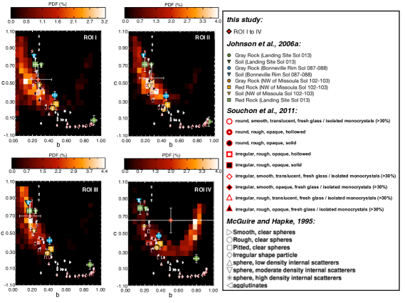
  Figure 10: Probability density map of the asymmetric parameter $b$ (horizontal axis) and the backscattering fraction $c$ (vertical axis) solutions from the last 500 iterations of the Bayesian inversion estimated at 750 nm obtained for the four selected ROIs. The grid is divided into 24 (vertical) x 20 (horizontal) square bins. The coloring gives the probability corresponding to each bin. Means and 2$\sigma$ uncertainties (red rhombus) are plotted too. The inversion solutions are plotted against the experimental $b$ and $c$ values pertaining to artificial particles measured by McGuire and Hapke (1995) and to natural particles measured by Souchon et al. (2011). The Gray Rock (circle), Red Rock (square) and Soil (triangle) units from Pancam sequences at Landing Site (green), Bonneville Rim (blue) and NW of Missoula (orange) estimated at 753 nm (except for the Red Rock unit at the Landing Site which is constrained at 754 nm) (Johnson et al., 2006a) are plotted here.

• Macroscopic roughness: Means and uncertainties as well as the PDF of the macroscopic roughness $\bar{\theta}$ obtained for each selected ROI are presented in Figure 11. The parameter $\bar{\theta}$ of all selected ROIs, estimated from CRISM measurements is consistent with the Soil unit found at the Landing Site and at NW of Missoula (cf. Figure 11). By contrast, this parameter indicates a rougher surface than the soil unit found at Bonneville Rim which is consistent with Johnson et al. (2006a). At intercrater plains where the Landing site is situated, the greater proportion of small clasts in the soil (compared to the soils near Bonneville rim and Missoula area) may explain the rougher surface texture (Ward et al., 2005).

  

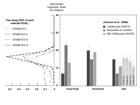
  Figure 11: Mean and uncertainties of the macroscopic roughness $\bar{\theta}$ estimated from Pancam measurements at 753 nm for different geological units at Landing Site (Sol 013), Bonneville Rim (Sol 087-088) and NW of Missoula (Sol 102-103) (Johnson et al., 2006a) compared to those estimated from CRISM measurements at 750 nm (note that the error bar represents 2$\sigma$ uncertainties) derived from 2-term HG models. The PDFs of the parameter $\bar{\theta}$ estimated from the last 500 iterations of the Bayesian inversion are also represented on the left side. This is helpful when mean and uncertainties are not representative of the PDF.

Two principal points from the previous comparison can be outlined. First, at the effective spatial scale achieved from space by CRISM for the photometric characterization (460 m), the surface behaves like the Soil units defined by Johnson et al. (2006a) and particularly like the Soil unit observed at the Landing Site. Second, the values of $\omega$ and $(b,c)$ resulting from our analysis are approximately inside the range of variation seen in Figures 9 and 10 for the Soil units at the three locations. This is not the case for the macroscopic roughness which is close to (within the error bars) the Soil unit values only for the Landing Site and Missoula area (cf. Figure 11). Consequently all photometric parameters retrieved following the methodology proposed in this article are consistent with the results arising from the analysis of Pancam measurements at Gusev provided that ROIs are associated to the proper soil unit. That means that the two independent investigations (the present work and the Johnson et al. (2006a)’s study) are cross-validated in the Gusev case.

4.1.3 Comparison with photometric estimates derived from orbital measurements by HRSC/MEx

Using HRSC imagery, which provides multi-angle data sets (up to five angular configurations by orbit) (McCord et al., 2007), Jehl et al. (2008) determined the regional variations of the photometric properties at the kilometer spatial scale across Gusev Crater and the south flank of Apollinaris Patera using several observations in order to cover a phase angle range from 5° to 95°. The photometric study was carried out without any atmospheric correction but ensuring that the atmospheric contribution was limited by selecting HRSC observations with AOT lower than 0.9. Jehl et al. (2008) applied an inversion procedure developed by Cord et al. (2003) based on the H93 version of Hapke’s model (equation 1). In Jehl et al. (2008)’s study, even photometric units were determined using a principal component analysis at 675 nm in which one of them corresponds to the Spirit landing site area. There is a robust overall first-order consistency between these photometric orbital estimates independently retrieved from HRSC and CRISM observations, particularly for ROIs I, II and III (see Table 7).

Table 7: Retrieved Hapke’s parameters and their standard deviation (the underconstrained parameters are indicated by "(-)") from CRISM measurement at 750 nm (present results) compared to those from HRSC measurements at 675 nm (Jehl et al., 2008). The yellow unit is associated to the Spirit landing site. The case 1 is the Hapke’s parameters determination when the opposition effect parameters are set free and the case 2, when the opposition effect is neglected, with phase angles larger than 20° (see Jehl et al. (2008) for more details).

Instrument	ROI or unit	$\omega$	$b$	$c$	$\bar{\theta}$	$B_{0}$	$h$
					(deg.)
CRISM	ROI I	0.71 (0.05)	0.22 (0.18)	0.54 (0.18)	15.78 (2.65)	0.49 (-)	0.54 (-)
	ROI II	0.72 (0.05)	0.27 (0.15)	0.56 (0.16)	15.62 (2.43)	0.49 (-)	0.52 (-)
	ROI III	0.69 (0.04)	0.19 (0.14)	0.66 (0.18)	13.96 (4.40)	0.50 (-)	0.53 (-)
	ROI IV	0.79 (0.07)	0.59 (0.27)	0.56 (0.16)	10.88 (5.11)	0.50 (-)	0.48 (-)
HRSC	case 1	0.72$\pm$0.02	0.06$\pm$0.02	0.34$\pm$0.06	18.5$\pm$1.5	0.73$\pm$0.07	0.75$\pm$0.13
	case 2	0.80$\pm$0.02	0.22$\pm$0.04	0.41$\pm$0.06	17.2$\pm$3.0	-	-

The principal point from the comparison between both orbital photometric results is that there is a robust overall first-order consistency between these photometric orbital estimates reached independently from HRSC and CRISM observations, particularly for ROIs I, II and III (see Table 7). However, in detail, two differences can be noted for the parameters $\omega$ and $c$ (see Table 7). In fact, the parameters $\omega$ and $c$ from CRISM measurements are respectively lower and higher than those determined from HRSC measurements. Moreover, the parameters $\omega$ and $c$ estimated from CRISM data set are more consistent with in situ measurements.These differences are explained by the use of an aerosol correction in the CRISM data whereas no correction was made in HRSC data. As a consequence, the contribution of bright and forward scattering aerosols in the HRSC measurements appeared to increase the apparent surface single scattering albedo and to decrease the surface backscattering fraction value.

4.2 Validation of Meridiani Planum

4.2.1 Comparison to experimental measurements on artificial particles

Our investigation shows that parameters $b$ and $c$ estimated from the inversion of both individual and combined (cf. Figure 12) CRISM FRTs are consistent with the L-shape defined from laboratory studies. However, the bidirectional reflectance sampling is not adequate to provide accurate estimation of the scattering parameters, even by combining up to three FRTs. In this case, according to parameters $b$ and $c$, the surface represented by ROI I is slightly forward scattering with a relatively broad lobe (low $b$ and $c$) which is consistent with artificial materials composed of round and clear sphere or agglutinates and close to irregular or round rough, opaque and solid natural particles (cf. Figure 12).

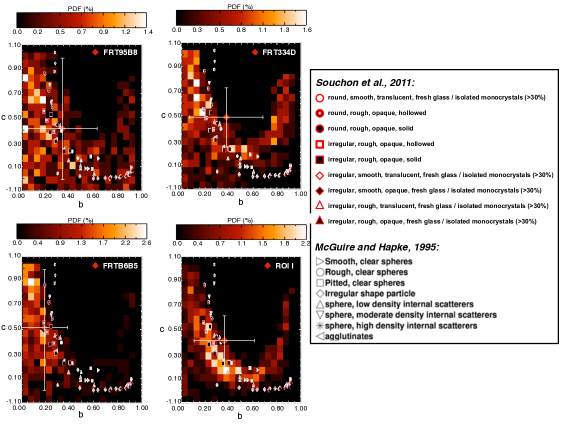
Figure 12: Same as Figure 8 for Meridiani Planum using observations FRT95B8, FRT334D and FRTB6B5 and their combination (ROI I).

4.2.2 Comparison to in situ measurements taken by Pancam/MER-Opportunity

Similar to the work done at the Spirit’s landing site, a photometric study was done at Meridiani Planum by using the Pancam instrument from Eagle crater to Purgatory ripple in (Johnson et al., 2006b). Units were defined, for example, as “Spherule soil” (typical soil with abundant spherules), “Bounce marks” (soil compressed by the airbags at the landing site), and “Outcrop rock” (bedrock). Our results are compared to two photometric sequences taken by Pancam that are near the selected ROI: South of Voyager (Sol 437-439) and Purgatory region (Sol 449-473) (cf. Figure 2). In addition to the Spherule soil unit, Johnson et al. (2006b) defined the soil class “Striped soil”, which characterizes soils with a striped appearance on the faces of some dune forms. Especially for the Purgatory region, large ripples were present and a specific class was defined. Bright soil deposits among the Striped soil unit were defined as a Dusty soil unit which was limited in spatial extent. Results are summarized in Table 8. In this article the photometric results are obtained from the combination of four FRT observations using the H93 version of the Hapke’s model. In this way, we use the same model as Johnson et al. (2006b).

Table 8: Retrieved Hapke’s parameters and their standard deviation (the unconstrained parameters are indicated by “(+,-)”) from the 2-term HG model for Sol 437-439 (Spherule Soil and Striped soil) and Sol 449-473 units (Spherule Soil, Striped Soil, Dusty Soil and Ripples) at 753 nm from Pancam onboard Opportunity (Johnson et al., 2006b).

Site	Unit	$\omega$	$\bar{\theta}$ (deg.)	$b$	$c$	Number	$g$ (deg.)
South of Voyager	Spherule soil	0.53 (+0.02, -0.07)	14 (+1, -2)	0.249 (+0.022, -0.031)	0.491 (+0.058, -0.057)	144	$\sim$5-140
(Sol 437-439)	Striped soil	0.56 (+0.01, -0.01)	15 (+1, -1)	0.305 (+0.010, -0.022)	0.353 (+0.033, -0.032)	119	$\sim$5-140
Purgatory region	Spherule soil	0.51 (+0.00, -0.01)	10 (+0, -1)	0.230 (+0.006, -0.007)	0.761 (+0.023, -0.013)	686	$\sim$0-135
(Sol 449-473)	Striped soil	0.52 (+0.24, -0.00)	11 (+0, -1)	0.117 (+0.011, -0.012)	1.000 (+, -)	104	$\sim$0-135
	Dusty soil	0.66 (+0.02,-0.02)	16 (+1,-1)	0.449 (+0.011,-0.020)	0.364 (+0.019,-0.053)	64	$\sim$0-135
	Ripples	0.52 (+0.01,-0.01)	9 (+1,-1)	0.255 (-0.008,-0.007)	0.434 (+0.023,-0.014)	234	$\sim$0-135

• Single scattering albedo: Figure 13 plots means and uncertainties as well as the PDF of the single scattering albedo $\omega$ of the selected ROI against the values of the Spherule Soil and Striped Soil units defined by Johnson et al. (2006b) at South of Voyager and the additional Dusty soil and Ripples units in the Purgatory region. The retrieved values of $\omega$ from CRISM are higher than those estimated from Pancam measurements except for the spatially sparse Dusty soil unit (first maximum of the PDF around 0.65).

  

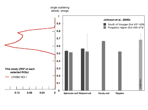
  Figure 13: Mean and uncertainties of the single scattering albedo $\omega$ estimated from Pancam measurements at 753 nm for different geological units at South of Voyager (Sol 437-439) and Purgatory region (Sol 449-473) (Johnson et al., 2006b) compared to those estimated from CRISM measurements at 750 nm (note that the error bar represents 2$\sigma$ uncertainties) derived from 2-term HG models. The PDFs of the parameter $\omega$ estimated from the last 500 iterations of the bayesian inversion are also represented on the left side. This is helpful when mean and uncertainties are not representative of the PDF (such as the PDF of the parameter $\omega$ for the ROI I which shows a bimodal distribution).

• Phase function: Figure 14 plots the asymmetric parameter $b$ and the backscattering fraction $c$ solutions of the Bayesian inversion for the ROI I in comparison to results of two photometric units (i.e., Spherule soil and Striped soil) from South of Voyager and three photometric units (Spherule soil, Dusty Soil and Ripples) for the Purgatory region. Note that the parameter $c$ is underconstrained in the Striped Soil unit in the Purgatory region area because of the relative lack of phase angle coverage ($\sim$45-110°). As mentioned in Subsection 3.2, parameters $b$ and $c$ are not well constrained in the CRISM case but exhibit slightly more forward scattering properties than at Gusev crater. This results is still potentially consistent with all units in Purgatory region and South of Voyager, except for the Spherule soil which exhibits more backscattering properties.

  

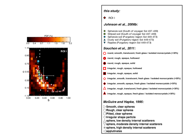
  Figure 14: Probability density map of the asymmetric parameter $b$ (horizontal axis) and the backscattering fraction $c$ (vertical axis) solutions from the last 500 iterations of the Bayesian inversion estimated at 750 nm obtained for the selected ROI. The grid is divided into 24 (vertical) x 20 (horizontal) square bins. The coloring gives the probability corresponding to each bin. Means and 2$\sigma$ uncertainties (red rhombus) are plotted too. The inversion solutions are plotted against the experimental $b$ and $c$ values pertaining to artificial particles measured by McGuire and Hapke (1995) and to natural particles measured by Souchon et al. (2011). The Spherule Soil (circle), Striped Soil (square), Ripple (triangle) and Dusty Soil (triangle) units from Pancam sequences at South of Voyager (green and Purgatory region (blue) estimated at 753 nm (Johnson et al., 2006b) are plotted here.

• Macroscopic roughness: Means and uncertainties as well as the PDF of the macroscopic roughness $\bar{\theta}$ modeled from CRISM data is higher than that retrieved at the South of Voyager and at Purgatory region (cf. Figure 15).

  

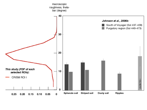
  Figure 15: Mean and uncertainties of the macroscopic roughness $\bar{\theta}$ estimated from Pancam measurements at 753 nm for different geological units at South of Voyager (Sol 437-439) and Purgatory region (Sol 449-473) (Johnson et al., 2006b) compared to those estimated from CRISM measurements at 750 nm (note that the error bar represents 2$\sigma$ uncertainties) derived from 2-term HG models. The PDFs of the parameter $\bar{\theta}$ estimated from the last 500 iterations of the Bayesian inversion are also represented on the left side. This is helpful when mean and uncertainties are not entirely representative of the PDF.

Two principal points from the previous comparison can be outlined. First, at the effective spatial scale achieved from space by CRISM for the photometric characterization (460 m), the surface behaves particularly like the Dusty Soil unit defined by Johnson et al. (2006b) at the Purgatory region: higher single scattering albedo, more forward scattering materials, and rougher surfaces. Second the photometric properties estimated from CRISM data are not strongly supported by those determined from Pancam. In fact, the selected ROI and the Pancam photometric sequences (South of Voyager and Purgatory region) are located several kilometers to the south of the Opportunity landing site where a geological transition region is observed. Indeed bright plains which exposed a smaller areal abundance of hematite, brighter fine-grained dust rich in nanophase iron oxides (such as in Gusev Crater plains) and a larger areal of bright outcrops are observed from orbital measurements (cf. Auxiliary Materials - Figure 1) compared to plains near the landing site (Arvidson et al., 2006). Inside the ROI I, even if the bright material unit does not seem to be the main geological unit at centimeter spatial scale, it seems to be more abundant from the orbit.

5 Discussion

The previous results show that the surface photometric parameters retrieved in this study are consistent with those derived from in situ measurements. This cross-validation demonstrates that MARS-ReCO is able to estimate accurately the surface bidirectional reflectance of Mars. Nevertheless one could question the significance of these estimates. Therefore, this section aims at testing the non-Lambertian surface hypothesis used by MARS-ReCO and the influences of the surface bidirectional reflectance sampling on the determination of the photometric parameters.

5.1 Non-Lambertian surface hypothesis

The compensation for aerosol contribution represents a great challenge for photometric studies. In planetary remote sensing, the Lambertian surface assumption is often adopted by the radiative atmospheric calculations that allow retrieval of surface reflectance (Vincendon et al., 2007; McGuire et al., 2008; Brown and Wolff, 2009; Wiseman et al., 2012). The surface reflectance is then assumed to be independent on geometry (i.e., the variation of TOA radiance with geometry is supposed to exclusively relate to aerosol properties). This hypothesis is generally used as it simplifies the radiative transfer modeling. However, it has been proved that most surface materials (e.g., minerals and ices) have an anisotropic non-Lambertian scattering behaviors (de Grenier and Pinet, 1995; Pinet and Rosemberg, 2001; Johnson et al., 2006a, b; Johnson et al., 2008; Lyapustin et al., 2010). Consequently, considering a Lambertian hypothesis can potentially create biases in the determination of the surface reflectance.

For the AOT estimate some assumptions regarding the surface properties were taken in Wolff et al. (2009)’s work. Indeed this method assumes a non-Lambertian surface to estimate the AOT by using a set of surface photometric parameters (Johnson et al., 2006a, b) that appears to describe the surface phase function adequately for both MER landing sites (roughly associated to the brighter or dusty soils). This assumption is qualitative but reasonable for several reasons enumerated by Wolff et al. (2009). However bias in the estimation of surface bidirectional reflectance can appear. For both MER landing sites it seems from Wolff et al. (2009)’s work that the AOT retrievals are overall consistent with optical depths returned by the Pancam instrument (available via PDS).

In order to test whether or not the non-adoption of a Lambertian hypothesis improves the quality of the retrieved surface reflectance, we compare the surface reflectance and the surface photometric parameters retrieved by a radiative transfer-based atmospheric correction technique that adopts a Lambertian assumption for the surface (Douté, S., 2009) and those given by MARS-ReCO (Ceamanos et al., 2013).

Figure 16 presents the initial TOA reflectance and the surface reflectance derived from both atmospheric correction techniques as a function of the phase angle. As can be seen, the main difference is observed at high phase angle (greater than 90°) where lower BRF are estimated in the case of the Lambertian method. This difference can be explained by the non-Lambertian assumption of the surface by MARS-ReCO. Table 9 presents the photometric parameters retrieved from the surface bidirectional reflectance estimated from both techniques. First, solutions are found for the parameters $\omega$, $b$, $c$ and $\bar{\theta}$ with higher standard deviations from the Lambertian method. Second, higher $b$ is observed from the Lambertian method which is not compatible with the in situ photometric results. This shows that the consideration of a non-Lambertian surface in the correction for aerosol contribution by MARS-ReCO is needed for the determination of accurate surface bidirectional reflectance and thus for the estimation of accurate surface photometric parameters.

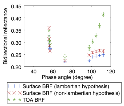
Figure 16: Photometric curves corresponding to ROI I of the FRT3192 observation and composed of ten angular configurations. The reflectance values (in BRF units) are extracted at the TOA (green asterisk), and at the surface after correction for atmospheric contribution. The latter takes into account a non-Lambertian surface hypothesis using MARS-ReCO (red crosses) and a Lambertian surface assumption (blue plus sign) (see details in Subsection 5.1). In the three cases we plot error bars corresponding to the $1\sigma$ uncertainty.

Table 9: Retrieved Hapke’s parameters ($\omega$, $b$, $c$, $\bar{\theta}$ in degree, $B_{0}$, $h$) and their standard deviation (the underconstrained parameters are indicated by "(-)") from CRISM measurement at 750 nm using our Bayesian inversion assuming (i) a non-Lambertian assumption (MARS-ReCO) (Ceamanos et al., 2013) and (ii) a Lambertian hypothesis (Douté, S., 2009) for the surface. The Hapke’s photometric parameters corresponding to the ROI I are retrieved by Bayesian inversion as well as the non-uniform criterion $k$. ($nb$: number of angular configurations, $g$: phase angle range in degree)

ROI	FRT	AOT	$\omega$	$b$	$c$	$\bar{\theta}$	$B_{0}$	$h$	$nb$	$g$
			$k$	$k$	$k$	$k$	$k$	$k$
ROI I	3192 (non-lamb. hypo.)	0.33$\pm$0.04	0.68 (0.06)	0.17 (0.20)	0.62 (0.20)	11.62 (3.98)	0.52 (-)	0.52 (-)	10	$\sim$56-112
			1.00	1.92	0.96	1.00	0.24	0.12
	3192 (lamb. hypo.)	0.33$\pm$0.04	0.74 (0.08)	0.46 (0.32)	0.64 (0.17)	12.43 (4.86)	0.52 (-)	0.50 (-)	10	$\sim$56-112
			0.99	1.12	0.74	0.98	0.25	0.03

5.2 Influences of the surface bidirectional reflectance sampling on the determination of the photometric parameters

The accuracy of the determination of Hapke’s parameters $\omega$, $b$, $c$, $\bar{\theta}$, $B_{0}$ and $h$ highly depends on the quality and the representativeness of the surface bidirectional reflectance used for their estimation. Indeed, for a given phase angle range, the estimation of all parameters is essentially controlled by the degree to which the angular space (incidence, emergence, azimuth and consequently phase angles) is covered rather than by the number of available angular configurations (Souchon et al., 2011). Also, a large phase angle domain is required. In fact, certain photometric parameter are sensitive to the availability of low and high phase angle values. First, the opposition effect is visible only with phase angle values less than 20°. Second, for an accurate determination of the macroscopic roughness, observations that span from small phase angle out to phase angle above 90° is needed (Helfenstein, 1988). Finally, materials with strong backscattering or forward scattering properties require the consideration of large phase angles, ideally greater than 140° (Kamei and Nakamura, 2002; Shkuratov et al., 2007; Shepard and Helfenstein, 2011; Helfenstein et al., 1991).

As presented previously (Subsection 2.1.1), CRISM targeted observations are composed of eleven images which are characterized by a constant incidence angle and eleven different emergence angles. Two modes of relative azimuth are used corresponding to the inbound and outbound portions of the spacecraft trajectory. Based on laboratory experiments performed under a given incidence angle, Souchon (2012) showed that the photometric parameters are determined with a good reliability under the condition of varied emergence and azimuth angles, resulting in varied phase angle values. However, each CRISM observation has intrinsically limited azimuthal and emergence coverage, which affects the determination of all the photometric parameters such as the opposition effect parameters, $B_{0}$ and $h$, the phase function parameters, $b$ and $c$, and the macroscopic roughness, $\bar{\theta}$. The solution used in the present study is to combine several targeted observations with different illumination conditions taken at different times in a year (because of the MRO sun-synchronous orbit) in order to enrich as much as possible the phase angle range by adding low and high phase angles. Nevertheless, low (less than 20°) and high (greater than 120°) phase angle values are not available here.

Thanks to Bayesian inversion, the shape of the a posteriori PDF is known and will inform us whether the bidirectional reflectance sampling is sufficient to estimate accurate photometric parameters. In fact, a uniform or bimodal PDF are the consequence of a lack of the bidirectional reflectance sampling as confirmed by synthetic tests.

Note that the surface bidirectional sampling also influences the AOT estimate notably through the determination of the single scattering albedo. Large AOT error bars are related to CRISM targeted observations presenting limited geometries (Wolff et al., 2009). However, the surface bidirectional reflectance estimated by MARS-ReCO is sensitive to the accuracy of the AOT input (Ceamanos et al., 2013).

5.3 Comparison of surface photometric results from Pancam versus CRISM

The differences regarding the acquisition geometries between Pancam and CRISM can influence the determination of the photometric properties. Ideally, in order to properly compare both results, the bidirectional reflectance sampling should be the same. However, this cannot be achieved because of technical constraints on the acquisition of the bidirectional reflectance measurements in the case of a spaceborne instrument and an in situ vehicle, respectively. In addition, the atmospheric contribution does not affect the observation in the same manner. In the orbital case the light travels twice across the atmosphere while in the in situ case, it only travels once before reaching the sensor.

Comparison of orbital photometric results to in situ photometric results demonstrates two main differences arising from different acquisition modes. The first comes from the sampling of the bidirectional reflectance. Pancam acquires a photometric sequence by varying the illumination angles (observations acquired at several times of day) and by varying the local azimuth and emission angles among similar units to order to enrich the phase angle range.

The second difference comes from the spatial scale that is accessible. CRISM photometric curves are obtained at the hectometric spatial scale on an extended area whereas Pancam observes at the centimeter spatial scale. Some characteristics of the surface can be observed at a hectometric scale but not at centimeter scale and conversely. From the ground, Pancam is able to distinguish rocks and soils with relatively high variability, whereas CRISM observes extended areas for which the variability of rocks and soils may appear relatively reduced. Despite these differences, the choice is made here to consider the Pancam in situ photometric results as the ground truth, taken as a reference.

5.4 Interpretation of the retrieved photometric parameters from orbit

Consistent trends were found with regard to the in situ photometric results. At the hectometer-scale, the surface behaves like the Soil unit defined by Johnson et al. (2006a). The signal acquired by CRISM mixes several contributions coming from distinct surface materials occurring at the sub-pixel level. This mixing can be (i) linear or (ii) non-linear. In the case of linear mixing (geographic mixing), the measured signal is a linear sum of all the radiated energy curves of materials making up the pixel. Consequently, the consistency of our results with the Soil unit behavior can be due to their dominant relative abundance within the CRISM pixel. In the case of non-linear mixing, the signal measured is the result of a non-linearly weighted combination of signals coming from different units. In both cases, the apparent consistency with the Soil unit could be coincidental.

Previous orbital observations acquired at the MER landing sites gave several clues concerning its physical and chemical properties. This information can be used to validate the present photometric results to provide a better understanding of the geological meaning of the estimated photometric properties. First, we compare our results to the albedo estimates by Thermal Emission Spectrometer (TES) instrument. Spirit landed in a relatively dark streak feature which is composed of hundreds of dark-toned, small, sub-parallel streaks created by dust devils, roughly oriented NW-SE. This feature is characterized by low albedo values (between 0.16 and 0.22) (Martinez-Alonso et al., 2005). Pancam in situ analysis (Bell et al, 2004; Farrand et al., 2006) and coupled OMEGA measurements and Spirit data (Lichtenberg et al., 2007) show that the Spirit landing site is mainly composed of soil deposits sprinkled with small rocks interspersed with dust deposits composed of fine-grained nanophase iron-oxide-rich. These results are consistent with the intermediate single scattering albedo estimates modeled from CRISM observations ($\omega\sim 0.68$). Meridiani Planum is characterized by a low albedo estimated at 0.09-0.19 (Mellon et al., 2000). Dust-free dark sand surface is mainly observed on the Meridiani Planum landing site. However the intermediate single scattering albedo value modeled from CRISM dataset is more consistent with bright plains which exposed a smaller areal abundance of hematite, brighter fine-grained dust rich in nanophase iron oxides (such as in Gusev Crater plains) and a larger areal of bright outcrops are observed several kilometers to the south of the Opportunity landing site from orbital measurements (Arvidson et al., 2006).

Second, we compare our results to the thermal inertia (TI) estimated by THermal EMission Imaging System (THEMIS) images. This is a measure of the resistivity of surface materials to a change in temperature which is function of the particle size, bulk density and cohesion. The intermediate THEMIS-derived TI at Gusev landing site (186-347 SI, 3x6 km resolution, (Martinez-Alonso et al., 2005)) suggests that the surface is dominated by unconsolidated materials (cohesionless surface) which is consistent with the photometric estimates. This shows that the surface dominantly behaves like the Soil unit, particularly those observed at the Landing site which exhibit more small clasts in soil. At Meridiani landing site, lower THEMIS-derived TI are found (i.e., 175 SI, 3x6 km resolution, (Jakosky et al., 2006)) suggests that the surface is dominated by more fine-grained materials. Those pieces of information are consistent with the CRISM-derived photometric estimates showing that the area has similar properties as the Soil unit.

Even if consistent trends were found, one difference is observed with regard to the in situ photometric results. The difference concerns the macroscopic roughness $\bar{\theta}$. At Gusev Crater, the intermediate values of $\bar{\theta}$ conjugated to the presence of more small clasts on soil (Ward et al., 2005; Johnson et al., 2006a) suggests that the parameter $\bar{\theta}$ is mainly sensitive to micro-structure. In contrast, slightly rougher soil was modeled from CRISM data at Meridiani Planum. This outcome can be explained by (i) the presence of rocks but very few rocks are observed (Golombek et al., 2005) and/or (ii) the presence of less than 1 cm-hematite-rich concretions (Calvin et al., 2008) and/or (iii) the presence of morphological structures such as cm- high ripples (Golombek et al., 2010). The second and third explanations could be responsible for the roughness measured at hectometer scale, suggesting that the parameter $\bar{\theta}$ is sensitive to both the specific local micro- and macro-structure. At the Gusev plain, it seems that the surface roughness is dominated by small clasts in soils, whereas, at Meridiani Planum it is dominated by the soil particles (concretions) and ripples.

6 Conclusions

CRISM observations acquired over the MER-Spirit and MER-Opportunity landing sites allow us to validate the accuracy of (i) the Martian surface bidirectional reflectance estimated by the procedure named MARS-ReCO developed by Ceamanos et al. (2013) and (ii) the determined Martian photometric parameters, by comparing our results to the in situ photometric results modeled from data taken by the Pancam instrument on-board both rovers. Indeed, Hapke’s parameters ($\omega$, $\bar{\theta}$, $b$ and $c$) estimated from CRISM measurements (using a combination of CRISM multi-angle images after individually by applying to each FRT observation the MARS-ReCO atmospheric correction procedure), are mainly consistent with parameters modeled from in situ measurements taken at the Spirit and Opportunity landing sites. The innovative assumption of a non-Lambertian surface is used in our methodology to accurately estimate intrinsic surface photometric properties from space. Our results appear to improve (i) those achieved in HRSC-based photometric studies, in which no aerosol correction was used, and (ii) those estimated from surface bidirectional reflectance derived from atmospheric correction assuming a Lambertian surface, as they better compare with the in situ Pancam results. This outcome of our study shows that MARS-ReCO gives access to consistent surface bidirectional reflectance. As a consequence, surface photometric parameters can be reliably estimated from CRISM observations, provided that the atmospheric conditions are not turbid. As presented previously, the AOT values derived from Wolff et al. (2009)’s work are estimated with assumptions concerning the surface properties, imposed to be similar as MER observations at both landing sites. Further developments could lead to the joint estimation of AOT and surface bidirectional reflectance by considering the full spectral dimension.

This presented approach may suffer from intrinsic limitations due to the scarcity of CRISM measurements with broad bidirectional reflectance sampling. However the combination of several CRISM observations alleviates this problem by improving the phase angle range thus better constraining the determination of photometric parameters. Furthermore, Since September, 2010, the inbound segment in targeted observations is absent due to problems of the instrument gimbal (Murchie, 2012). Only 6 angular configurations are still available after this date. Consequently, more targeted observations must be combined in order to compensate this limitation.

The presented methodology opens the possibility to map the surface bidirectional reflectance thus the spatial variations of the photometric parameters. The determination of the physical state of the surface materials (i.e., mean grain size, grain sphericity and grain heterogeneity, mean surface porosity and surface brightness) through the study of their photometric properties (phase function of the particle, single scattering albedo, surface roughness, and opposition effects) provides complementary information to composition. It has implications for the characterization of different types of terrain over Mars (i.e., extrusive and intrusive volcanic terrains, sedimentary terrains, impact craters) and for identification of surface temporal modifications (i.e., aeolian process, space weathering process). Moreover, the present work has implications for spectroscopic interpretation as it gives information about the particle (i.e., size) and grain organization which have significant influence on spectral properties (Poulet and Erard, 2004).

In future work, both challenges of map creation and improvements for non-flat terrains shall be taken into account, with a particular emphasis on the complex handling of local slope effects which is not straightforward in the case of multiple reflection between surface facets. Note that MARS-ReCO may be used for mapping the photometric properties of the Martian surface even when using a single CRISM targeted observation. In this case, however, the photometric inversion should be focused to retrieve only single scattering albedo for the best surface bidirectional reflectance sampling. Furthermore, use of a single-lobed Henyey-Greenstein function would reduce the number of unknown photometric parameters and therefore could allows us to constrain the asymmetry parameter besides the single scattering albedo. Likewise, laboratory studies bearing on the photometric behavior of natural surfaces under controlled conditions and under a large range of observational geometries (Souchon et al., 2011) are necessary to better document and interpret the variations of the photometric parameters in relation with surface geological processes such as eolian, aqueous and impact processes.

Appendix A

Non-uniform PDF

Central moments $\mu_{n}$ (such as the variance $\mu_{2}$ of order two) are commonly used for statistical purpose while cumulants $k_{n}$ have the advantage to present unbiased statistical estimator for all orders (Fisher, 1930). Also, the first three cumulants are equivalent to the central moments. For a random variable following the PDF $f(x)$ in (0,1), the cumulant generating function is:

$$\Phi(t)=\ln TF\left\{f(x)\right\}=\ln\intop_{0}^{1}e^{itx}f(x)dx$$ (9)

Cumulants of order $n$ are defined by :

$$k_{n}=\frac{\partial^{n}\Phi(t)}{\partial it^{n}}+o(t)$$ (10)

The first four cumulants of a uniform PDF are:

$$k_{1}=\frac{1}{2}=\mu_{1}$$ (11)

$$k_{2}=\frac{1}{12}=\mu_{2}$$ (12)

$$k_{3}=0=\mu_{3}$$ (13)

$$k_{4}=-\frac{1}{120}=\mu_{4}-3\left(\mu_{2}\right)^{2}$$ (14)

Thus we propose to estimate the non-uniformity of the results of the inversion with:

$$k=max\mid\frac{k_{1}-12}{12},\frac{k_{2}-112}{112},\frac{k_{3}}{160},\frac{k_{4}+1120}{1120}\mid$$ (15)

We perform 10,000 uniform random vectors of 500 samples (identical to the inversion procedure). Since the maximum is $k$=0.47 for the most extreme event, we propose to have non-uniform PDF for $k$>0.5. For the inversion purpose, since the a priori PDF’s on the parameters are uniform if the results of the inversion on one parameter has $k$<0.5, we conclude that this parameters is not constrained by the observations.

References

- Arvidson et al. (2006) Arvidson, R. E., F. Poulet, R. V. Morris, J.-P. Bibring, I. Bell, J. F., S. W. Squyres, P. R. Christensen, G. Bellucci, B. Gondet, B. L. Ehlmann, W. H. Farrand, R. L. Fergason, M. Golombek, J. L. Griffes, J. Grotzinger, E. A. Guinness, K. E. Herkenhoff, J. R. Johnson, G. Klingelhofer, Y. Langevin, D. Ming, K. Seelos, R. J. Sullivan, J. G. Ward, S. M. Wiseman, and M. Wolff, Nature and origin of the hematite-bearing plains of terra meridiani based on analyses of orbital and mars exploration rover data sets, J. Geophys. Res., 111, E12S08, doi:10.1029/2006JE002728, 2006.
- Bell III et al. (1999) Bell III, J. F., M. J. Wolff, T. C. Daley, P. B. Crisp, S. W. Lee, J. T. Trauger, and R. W. Evans, Near-infrared imaging of Mars from HST: Surface reflectance, photometric properties, and implications for MOLA data, Icarus, 138, 25–35, doi:10.1006/icar.1998.6057, 1999.
- Bell et al (2004) Bell, J. F. et al, Pancam multispectral imaging results from the Spirit rover at Gusev Crater, Science, 305, no. 5685, 800–806, doi:10.1126/science.1100175, 2004.
- Brown and Wolff (2009) Brown, A. J., and M. J. Wolff, Atmospheric modeling of the Martian polar regions: One Mars year of CRISM EPF observations of the south pole, Lunar Planet. Sci., abstract 1675, 2009.
- Calvin et al. (2008) Calvin, W. M. et al., Hematite spherules at Meridiani: Results from MI, Mini-TES and Pancam, J. Geophys. Res., 113, E12S37, doi:10.1029/2007JE003048, 2008.
- Ceamanos et al. (2013) Ceamanos, X., S. Douté, J. Fernando, F. Schmidt, P. Pinet, and A. Lyapustin, Surface reflectance of mars observed by CRISM/MRO: 1. multi-angle approach for retrieval of surface reflectance from crism observations (MARS-ReCO), J. Geophys. Res. in press, doi:10.1029/2012JE004195, 2013.
- Chandrasekhar (1960) Chandrasekhar, S., Radiative Transfer, Dover, Mineola, NY., 1960.
- Cheng and Domingue (2000) Cheng, A., and D. L. Domingue, Radiative transfer models for light scattering from planetary surfaces., J. Geophys. Res., 105 (E4), 9477–9482, doi:10.1029/1999JE001170, 2000.
- Clancy and Lee (1991) Clancy, R. T., and S. W. Lee, A new look at dust and clouds in the Mars atmosphere: analysis of Emission-Phase-Function sequences from global Viking IRTM observations, Icarus, 93, 135–158, doi:10.1016/0019-1035(91)90169-T, 1991.
- Clancy et al. (2003) Clancy, R. T., M. J. Wolff, and P. R. Christensen, Mars aerosol studies with the MGS TES emission phase function observations: Optical depths, particle sizes, and ice cloud types versus latitude and solar longitude, J. Geophys. Res., E9 5098, doi:10.1029/2003JE002058, 2003.
- Cord et al. (2003) Cord, A. M., P. C. Pinet, Y. Daydou, and S. D. Chevrel, Planetary regolith surface analogs: optimized determination of Hapke parameters using multi-angular spectro-imaging laboratory data, Icarus, 165, 414–427, doi:10.1016/S0019-1035(03)00204-5, 2003.
- de Grenier and Pinet (1995) de Grenier, M., and P. C. Pinet, Near-opposition martian limb-darkening: quantification and implication for visible-near-infrared bidirectional reflectance studies, Icarus, 115, 354–368, doi:10.1006/icar.1995.1103, 1995.
- Douté and Schmitt (1998) Douté, S., and B. Schmitt, A multilayer bidirectional reflectance model for the analysis of planetary surface hyperspectral images at visible and near-infrared wavelengths, J. Geophys. Res., 103, 31,367–31,389, doi:10.1029/98JE01894, 1998.
- Douté, S. (2009) Douté, S., Retrieving Mars surface reflectance from OMEGA/MEx imagery, IEEE Workshop on Hyperspectral Image and Signal Processing : Evolution in Remote Sensing, 2009.
- Farrand et al. (2006) Farrand, W. H., J. F. Bell III, J. R. Johnson, S. W. Squyres, J. Soderblom, and D. Ming, Spectral variability among rocks in visible and near-infrared multispectral Pancam data collected at Gusev Crater: Examinations using spectral mixture analysis and related techniques, J. Geophys. Res., 111, E02S15, doi:10.1029/2005JE002495, 2006.
- Fisher (1930) Fisher, R. A., The Genetical Theory Of Natural Selection, Clarendon Press, 1930.
- Golombek et al. (2005) Golombek, M. P. et al., Assessment of Mars Exploration Rover landing site predictions, Nature, 436, 44–48, doi:10.1038/nature03600, 2005.
- Golombek et al. (2010) Golombek, M., K. Robinson, A. McEwen, B. Bridges, N. Ivanov, L. Tornabene, and S. R., Constraints on ripple migration at Meridiani Planum from Opportunity and HiRISE observations of fresh craters, J. Geosphys. Res., 115, E00F08, doi:10.1029/2010JE003628, 2010.
- Grynko and Shkuratov (2007) Grynko, Y., and Y. Shkuratov, Ray tracing simulation of light scattering by spherical clusters consisting of particles with different shapes, Journal of Quantitative Spectroscopy & Radiative Transfer, 106, 56–62, doi:10.1016/j.jqsrt.2007.01.005, 2007.
- Guinness et al. (1997) Guinness, E. A., R. E. Arvidson, I. H. D. Clark, and M. K. Shepard, Optical scattering properties of terrestrial varnished basalts compared with rocks and soils at the Viking Lander sites, J. Geophys. Res., 102, 28,687–28,703, doi:10.1029/97JE03018, 1997.
- Hapke (1981a) Hapke, B., Bidirectional reflectance spectroscopy 1. theory, J. Geophys. Res., 86, 3039–3054, doi:10.1029/JB086iB04p03039, 1981a.
- Hapke (1981b) Hapke, B., and E. Wells, Bidirectional Reflectance Spectroscopy 2. Experiments and Observations, J. Geophys. Res., 86, 3055–3060, 1981b.
- Hapke (1984) Hapke, B., Bidirectional Reflectance Spectroscopy 3. Correction for Macroscopic Roughness, Icarus, 59, 41–59, doi:10.1016/0019-1035(84)90054-X, 1984.
- Hapke (1986) Hapke, B., Bidirectional Reflectance Spectroscopy 4. The Extinction Coefficient and the Opposition Effect, Icarus, 67, 264–280, doi:10.1016/0019-1035(86)90108-9, 1986.
- Hapke (1993) Hapke, B., Theory of Reflectance and Emittance Spectroscopy, Cambridge Univ. Press, New York, 1993.
- Hapke (2002) Hapke, B., Bidirectional Reflectance Spectroscopy 5. The Coherent Backscatter Opposition Effect and Anisotropic Scattering, Icarus, 157, 523–534, doi:10.1006/icar.2002.6853, 2002.
- Hapke (2008) Hapke, B., Bidirectional reflectance spectroscopy 6. effects of porosity, Icarus, 195, 918–926, doi:10.1016/j.icarus.2008.01.003, 2008.
- Hartman and Domingue (1998) Hartman, B., and D. Domingue, Scattering of light by individual particles and the implications for models of planetary surfaces, Icarus, 131, 421–448, doi:10.1016/j.jqsrt.2011.04.006, 1998.
- Helfenstein (1988) Helfenstein, P., The geological interpretation of photometric surface roughness, Icarus, 73, 462–481, doi:10.1016/0019-1035(88)90056-5, 1988.
- Helfenstein et al. (1991) Helfenstein, P., U. A. Bonne, S. Stolovy, and J. Veverka, Laboratory photometric measurements of particulate soils out to very large phase angles., Reports of Planetary Geology and Geophysics Program - 1990, NASA-TM-4300, 280–282, 1991.
- Jakosky et al. (2006) Jakosky, B. M. et al., Thermophysical properties of the MER and Beagle II landing site regions on Mars, J. Geophys. Res., 111, E08,008, doi:10.1029/2004JE002320, 2006.
- Jehl et al. (2008) Jehl, A., et al., Gusev photometric variability as seen from orbit by HRSC/Mars-express, Icarus, 197, 403–428, doi:10.1016/j.icarus.2008.05.022, 2008.
- Johnson et al. (1999) Johnson, J. R. et al., Preliminary results on photometric properties of materials at the Sagan Memorial Station, Mars, J. Geophys. Res., 104, 8809–8830, doi:doi:10.1029/98JE02247, 1999.
- Johnson et al. (2006a) Johnson, J. R. et al., Spectrophotometric properties of materials observed by Pancam on the Mars Exploration Rovers: 1. Spirit, J. Geophys. Res., 111, E02S14, doi:10.1029/2005JE002494, 2006a.
- Johnson et al. (2006b) Johnson, J. R. et al., Spectrophotometric properties of materials observed by Pancam on the Mars Exploration Rovers: 2. Opportunity, J. Geophys. Res., 111, E12S16, doi:10.1029/2006JE002762, 2006b.
- Johnson et al. (2006c) Johnson, J. R. et al., Radiative transfer modeling of dust-coated Pancam calibration target materials: Laboratory visible/near-infrared spectrogoniometry, J. Geophys. Res., 111, E12S07, doi:10.1029/2005JE002658, 2006c.
- Johnson et al. (2008) Johnson, J. R., J. F. Bell, P. Geissler, W. M. Grundy, E. A. Guinness, P. C. Pinet, and J. Soderblom, The martian surface, chap. physical properties of the martian surface from spectrophotometric observations, Cambridge University Press, 2008.
- Kamei and Nakamura (2002) Kamei, A., and A. M. Nakamura, Laboratory study of the bidirectional reflectance of powdered surfaces: On the asymmetry parameter of asteroid photometric data, Icarus, 156, 551–561, doi:10.1006/icar.2002.6818, 2002.
- Lichtenberg et al. (2007) Lichtenberg, K. A. et al., Coordinated analyses of orbital and Spirit Rover data to characterize surface materials on the cratered plains of Gusev Crater, Mars, J. Geophys. Res., 112, E12S90, doi:10.1029/2006JE002850, 2007.
- Lucht et al. (2000) Lucht, W., C. B. Schaaf, and A. H. Strahler, An algorithm for the retrieval of albedo from space using semiempirical BRDF models, IEEE Transaction on Geoscience and Remote Sensing, 38(2), 977–998, 2000.
- Lyapustin et al. (2010) Lyapustin, A., C. K. Gatebe, R. Kahn, R. Brandt, J. Redemann, et al., Analysis of snow bidirectional reflectance from ARCTAS Spring-2008 Campaign, Atmospheric Chemistry and Physics, 10, 4359–4375, doi:10.5194/acp-10-4359-2010, 2010.
- Martinez-Alonso et al. (2005) Martinez-Alonso, S., B. M. Jakosky, M. T. Mellon, and N. E. Putzig, A volcanic interpretation of Gusev Crater surface materials from thermophysical, spectral, and morphological evidence, J. Geophys. Res., 110, E01,003, doi:10.1029/2004JE002327, 2005.
- McCord et al. (2007) McCord, J. B. A., T.B., et al., The Mars Express High Resolution Stereo Camera spectrophotometric data: Characteristics and science analysis., J. Geophys. Res., 112, E06,004, doi:10.1029/2006JE002769.E06004, 2007.
- McGuire and Hapke (1995) McGuire, A., and B. Hapke, An experimental study of light scattering by large irregular particles, Icarus, 113, 134–155, 1995.
- McGuire et al. (2008) McGuire, P. C., M. J. Wolff, M. D. Smith, R. E. Arvidson, S. L. Murchie, et al., MRO/CRISM retrieval of surface lambert albedos for multispectral mapping of Mars with DISORT-based radiative transfer modeling: Phase 1 - Using historical climatology for temperatures, aerosol optical depths, and atmospheric pressures, IEEE Transactions on Geoscience and Remote Sensing, 46 (12), 4020–4040, 2008.
- Mellon et al. (2000) Mellon, M. T., B. M. Jakosky, H. H. Kieffer, and P. R. Christensen, High-Resolution Thermal Inertia Mapping from the Mars Global Surveyor Thermal Emission Spectrometer, Icarus, 148, 437–455, doi:10.1006/icar.2000.6503, 2000.
- Mishchenko et al. (1999) Mishchenko, M., J. M. Dlugach, E. G. Yanovitskij, and N. T. Zakharova, Bidirectional reflectance of flat, optically thick particulate layers: An efficient radiative transfer solution and applications to snow and soil surfaces., J. Quant. Spectrosc. Radiat. Trans., 63, 409–432, doi:10.1016/S0022-4073(99)00028-X, 1999.
- Mosegaard and Tarantola (1995) Mosegaard, K., and A. Tarantola, Monte Carlo sampling of solutions to inverse problems, J. Geophys. Res., 100, 12,431–12,447, 1995.
- Murchie et al. (2007) Murchie, S. et al., Compact Reconnaissance Imaging Spectrometer for Mars (CRISM) on Mars Reconnaissance Orbiter (MRO), J. Geophys. Res., 112, E05S03, doi:10.1029/2006JE002682, 2007.
- Murchie (2012) Murchie, S., CRISM on MRO - instrument and investigation overview, in MRO/CRISM Data Users’ Workshop, The Woodlands, TX, 2012.
- Pinet and Rosemberg (2001) Pinet, P., and C. Rosemberg, Regional photometry and spectral albedo of the eastern hemisphere of Mars in the 0.7-1 micron domain, Lunar Planet. Sci., abstract 1640, 2001.
- Pinet et al. (2005) Pinet, P. C., et al., Derivation of Mars surface scattering properties from OMEGA spot pointing, Lunar Planet. Sci., XXXVI, abstract 1694, 2005.
- Poulet and Erard (2004) Poulet, F., and S. Erard, Nonlinear spectral mixing: Quantitative analysis of laboratory mineral mixtures, J. Geophys. Res., 109, E02,009, doi:10.1029/2003JE002179, 2004.
- Seelos et al. (2011) Seelos, F. P., S. Murchie, D. Humm, O. S. Barnouin, F. Morgan, H. W. Taylor, C. Hash, and T. C. Team, CRISM data processing and analysis products update - calibration, correction, and visualization, Lunar Planet. Sci., XXXXII, abstract 1438, 2011.
- Shaw et al. (2012) Shaw, A., R. E. Arvidson, M. J. Wolff, F. P. Seelos, S. M. Wiseman, and S. Cull, Determining surface roughness and additional terrain properties: unsig opportunity mars rover results to interpret orbital data for extended mapping, Lunar Planet. Sci., XXXXIII, abstract 1644, 2012.
- Shepard and Helfenstein (2007) Shepard, M. K., and P. Helfenstein, A test of the Hapke photometric model,, J. Geophys. Res., 112, E03,001, doi:10.1029/2005JE002625., 2007.
- Shepard and Helfenstein (2011) Shepard, M. K., and P. Helfenstein, A laboratory study of the bidirectional reflectance from particulate samples, Icarus, 215, 526–533, doi:10.1016/j.icarus.2011.07.033, 2011.
- Shkuratov and Starukhina (1999) Shkuratov, Y., and L. Starukhina, A model of spectral albedo of particulate surfaces: implications for optical properties of the Moon, Icarus, 137, 235–246, doi:10.1006/icar.1998.6035, 1999.
- Shkuratov et al. (2007) Shkuratov, Y., S. Bondarenko, V. Kaydash, G. Videen, O. Munoz, and H. Volten, Photometry and polarimetry of particulate surfaces and aerosol particles over a wide range of phase angles, Jounal of Quantitative Spectroscopy & Radiative Transfer, 106, 487–508, doi:10.1016/j.jqsrt.2007.01.031, 2007.
- Soderblom et al. (2004) Soderblom, J. M., J. F. Bell, R. E. Arvidson, J. R. Johnson, M. J. Johnson, and F. P. Seelos, Mars Exploration Rover Pancam photometric data QUBs: Definition and example uses, AGU, 85(47) Fall Meet, Abstract P21A-0198., 2004.
- Souchon et al. (2011) Souchon, A. L., P. Pinet, S. Chevrel, Y. Daydou, D. Baratoux, K. Kurita, M. K. Shepard, and P. Helfenstein, An experimental study of Hapke’s modeling of natural granular surface samples, Icarus, 215, 313–331, doi:10.1016/j.icarus.2011.06.023, 2011.
- Souchon (2012) Souchon, A., Influence des phases amorphes dans la réponse optique des régolites planétaires : caractérisation des propriétés physiques et application a l’étude géologique de la lune, Ph.D. thesis, Univ. de Toulouse, France, 2012.
- Tarantola and Valette (1982) Tarantola, A., and B. Valette, Inverse problems=quest for information, J. Geophys. Res., 50, 159–170, 1982.
- Vincendon et al. (2007) Vincendon, M., Y. Langevin, F. Poulet, J.-P. Bibring, and B. Gondet, Recovery of surface reflectance spectra and evaluation of the optical depth of aerosols in the near-IR using a Monte Carlo approach: Application to the OMEGA observations of high-latitude regions of Mars, J. Geophys. Res., 112, E08S13, doi:10.1029/2006JE002845, 2007.
- Ward et al. (2005) Ward, J. G., R. E. Arvidson, and M. Golombek, The size-frequency and areal distribution of rock clasts at the Spirit landing site, Gusev Crater, Mars, Geophys. Res. Lett., 32, L11,203, doi:10.1029/2005GL022705, 2005.
- Wiseman et al. (2012) Wiseman, S. M., R. E. Arvidson, M. J. Wolff, R. V. Morris, F. P. Seelos, M. D. Smith, D. Humm, S. L. Murchie, and J. F. Mustard, Retrieval of atmospherically corrected CRISM spectra using radiative transfer modeling, Lunar Planet. Sci., XXXXIII, abstract 2146, 2012.
- Wolff et al. (2006) Wolff, M. J., M. D. Smith, R. T. Clancy, N. Spanovich, B. A. Whitney, M. T. Lemmon, J. L. Bandfiel, D. Bandfiel, A. Ghosh, G. Landis, P. R. Christensen, J. F. Bell III, and S. W. Squyres, Constraints on dust aerosols from the Mars Exploration Rovers using MGS overflights and Mini-TES, J. Geophys. Res., 111, E12S17, doi:10.1029/2006JE002786, 2006.
- Wolff et al. (2009) Wolff, M. J. et al., Wavelength dependence of dust aerosol single scaterring albedo as observed by the Compact Reconnaissance Imaging Spectrometer, J. Geophys. Res., 114, E00D64, doi:doi:10.1029/2009JE003350, 2009.
- Wolff et al. (2010) Wolff, M. J., R. T. Clancy, J. D. Goguen, M. C. Malin, and B. A. Cantor, Ultraviolet dust aerosol properties as observed by MARCI, Icarus, 208, 143–155, doi:10.1016/j.icarus.2010.01.010, 2010.