Inelastic collapse in one-dimensional driven systems under gravity

Abstract

We study the inelastic collapse in the one-dimensional $N$-particle systems in the situation where the system is driven from below under the gravity. We investigate the hard-sphere limit of the inelastic soft-sphere systems by numerical simulations to find how the collision rate per particle $n_{\rm coll}$ increases as a function of the elastic constant of the sphere $k$ when the restitution coefficient $e$ is kept constant. For the systems with large enough $N\gtrsim 20$, we find three regimes in $e$ depending on the behavior of $n_{\rm coll}$ in the hard-sphere limit: (i) uncollapsing regime for $1\geq e>e_{c1}$, where $n_{\rm coll}$ converges to a finite value, (ii) logarithmically collapsing regime for $e_{c1}>e>e_{c2}$, where $n_{\rm coll}$ diverges as $n_{\rm coll}\sim\log k$, and (iii) power-law collapsing regime for $e_{c2}>e>0$, where $n_{\rm coll}$ diverges as $n_{\rm coll}\sim k^{\alpha}$ with an exponent $\alpha$ that depends on $N$. The power-law collapsing regime shrinks as $N$ decreases and seems not to exist for the system with $N=3$ while, for large $N$, the size of the uncollapsing and the logarithmically collapsing regime decreases as $e_{c1}\simeq 1-2.6/N$ and $e_{c2}\simeq 1-3.0/N$ . We demonstrate that this difference between large and small systems exists already in the inelastic collapse without the external drive and the gravity.

I Introduction

The inelastic hard-sphere system is one of the simplest models of granular media. It consists of rigid spheres that interact with each other only through instantaneous inelastic collisions. Minimum ingredients of the granular systems are taken in this system, for which the efficient event-driven algorithms have been developed for molecular dynamics simulations Rapaport-1980 ; Luding-2004 ; Isobe-1999 as well as sophisticated kinetic theories for analytical study (see, for example, Ref. BrilliantovPoschel-2004 ).

With this idealization of the granular media, however, it has been known that infinite number of collisions among a finite number of particles can occur in a finite length of time. This phenomenon is called inelastic collapse BernuMazighi-1990 ; McNamaraYoung-1992 . Process of collisions involved in the inelastic collapse has been studied for one-dimensional (1-d) BernuMazighi-1990 ; McNamaraYoung-1992 and two-dimensional (2-d) systems McNamaraYoung-1994 ; McNamaraYoung-1996 ; ZhouKadanoff-1996 ; SchorghoferZhou-1996 ; AlamHrenya-2001 , and the conditions for the inelastic collapse have been obtained in some situations BernuMazighi-1990 ; McNamaraYoung-1992 ; McNamaraYoung-1994 ; McNamaraYoung-1996 ; ZhouKadanoff-1996 ; SchorghoferZhou-1996 .

One of the simplest cases is the freely cooling granular gas, in which the inelastic hard-sphere system develops freely without any external forces McNamaraYoung-1994 ; SchorghoferZhou-1996 . In the 2-d systems, it has been shown that the particles that partake in the inelastic collapse form a string like linear structure for the case of frictionless particles McNamaraYoung-1994 , while they form a string like zigzag pattern for the case of the frictional particles SchorghoferZhou-1996 . Another simple case is a simple shear flow, where the collapsing particles have been shown to form a linear string structure typically oriented along the direction $45^{\circ}$ from the flow direction AlamHrenya-2001 .

In the hard-sphere idealization, once the inelastic collapse occurs, the system cannot proceed further without additional assumptions for the dynamics, such as those in the contact dynamics JeanMoreau-1992 ; Moreau-1994 . A simple way to escape from this difficulty is to suppress the inelastic collapse by employing the velocity dependent restitution coefficient that goes to one as the colliding velocity goes to zero Goldmanetal-1998 ; Bizonetal-1998 . In actual systems with finite rigidity, the inelastic collapse should never occur.

Although the inelastic collapse is a singular behavior in the idealized system of the infinitely hard spheres with a constant restitution coefficient, its relevance to some physical behaviors has been suggested. In flowing configurations, it has been demonstrated by numerical simulations that there exists strong correlation between the force chain network and the chain like structure formed by particles that collide repeatedly with each other in the hopper flow FergusonChakraborty-2006 . The inelastic collapse has been also discussed in connection with the formation of correlation in the shear flow LoisLemaitreCarlson-2007 .

In order to study how the inelastic collapse affects system behaviors in physical situations, it is natural to investigate the soft sphere system with finite rigidity and see how the inelastic collapse appears in the hard-sphere limit. If you take, however, a simple limit of the infinite elastic constant with finite dissipation parameters, the resulting restitution coefficient tends to one, therefore the inelastic collapse does not occur. Thus the pertinent hard sphere limit for this purpose is the limit of infinite elastic constant with keeping the resulting restitution coefficient constant by making the dissipation parameter infinite.

Mitarai and Nakanishi studied such limit by examining the limiting behavior of the collision rate $n_{\rm coll}$ for the 2-d gravitational flow MitaraiNakanishi-2003 . The hard-sphere limit was taken as the limit of the infinite elastic constant $k$ with the restitution coefficient $e$ being kept constant. They found that $n_{\rm coll}$ converges to a finite value in the collisional flow regime, while it diverges as $n_{\rm coll}\sim k^{\alpha}$ as $k\to\infty$ in the frictional flow regime. The exponent $\alpha$ was estimated to be about $0.4$ in their case, i.e. the 2-d gravitational flow on a flat slope with ten layers of particles and the restitution coefficient $e=0.7$. More recently, Brewster et al. studied the three-dimensional gravitational flow and obtained $\alpha\simeq 0.25$ for the system with 90$\sim$100 layers of particles on a rough slope and $e=0.88$ BrewsterSilbertGrestLevine-2008 . Although the divergence of collision rate implies emergence of inelastic collapse in the hard-sphere limit, a simple consideration on exponentially decreasing collision time interval would give the logarithmic divergence, and the mechanism for the power law divergence has not been understood yet.

Motivated by these findings of the power law divergence in the gravitational slope flow, in this paper we take a closer look at the problem in an even simpler system, namely, a 1-d inelastic particle system under the gravity with an external excitation from a bottom of the system. The external excitation at the bottom is supposed to mimic the excitation by random collisions of particles with the slope in the gravitational flow, and our 1-d system is intended to capture only the particle motion perpendicular to the slope. By numerical simulations, we will show that even this simple model exhibits the power law divergence of the collision rate, $n_{\rm coll}\sim k^{\alpha}$.

This paper is organized as follows. In Sec. II, we begin by introducing our model and describe a method to study the hard-sphere limit of soft spheres in our simulations. The system with $N=3$ is analyzed to show the logarithmic behavior $n_{\rm coll}\sim\log k$ in the hard sphere limit. In Sec. III, after describing the simulation procedure, first we present the simulation results for the systems with small number of particles ($N=3\sim 6$); Only the logarithmic behavior in the hard sphere limit is observed for $N=3$ while the power law divergence regime appears for the larger system in the smaller $e$ region. Then we show the simulation results of systems with large number of particles ($N\gtrsim 20$) and demonstrate that there exist the three distinct regimes for the limiting behavior of $n_{\rm coll}$ in $e$. We discuss the origin of these limiting behaviors based on the simulation results of inelastic collapse in the 1-d free space. Summary and conclusion are given in Sec. IV.

II One-dimensional model of granular flow

II.1 Model

We consider the 1-d model by focusing the particle motion only perpendicular to the slope (see Fig. 1).

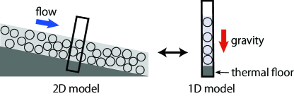
Figure 1: A schematic representation of relation between the granular slope flow and the 1-d driven system.

The particles are allowed to move only along the $z$-axis under the influence of gravity and the lowest particle is excited by the bottom floor.

Let us consider $N$ identical particles with mass $m$ and diameter $d$. The particles are numbered from the bottom starting with $i=1$, and can interact only with their adjacent particles through the soft-sphere interaction. The excitation by the random collision with the slope is represented by the thermal floor located at the bottom $z=0$. When the lowest particle ($i=1$) collides with the bottom, it comes off with a random velocity $v$ by the Maxwell-Boltzmann distribution

$$p(v)=\frac{mv}{k_{\rm B}T_{0}}\exp\left(-\frac{mv^{2}}{2k_{\rm B}T_{0}}\right),$$ (1)

where $T_{0}$ is temperature of the thermal floor and $k_{\rm B}$ is the Boltzmann constant.

The interaction between soft spheres is given by the so-called spring-dashpot model Duran-2000 ; Luding-2004 . Let $z_{i}$ and $v_{i}$ denote the coordinate and the velocity of particle $i$, respectively, then the overlap between the adjoining two particles $i$ and $i+1$ is given by $x_{i,i+1}\equiv d-(z_{i+1}-z_{i})$. The relative velocity between $i$ and $i+1$ is denoted as $v_{i,i+1}\equiv v_{i}-v_{i+1}={dx_{i,i+1}}/{dt}$. Then, the force $f_{i,i+1}$ exerted on particle $i$ by particle $i+1$ is given by

$$f_{i,i+1}=\left\{\begin{array}[]{@{\,}ll}-kx_{i,i+1}-Dmv_{i,i+1}&\mbox{(for $x_{i,i+1}>0$)},\\ 0&\mbox{(for $x_{i,i+1}\leq 0$)}.\end{array}\right.$$ (4)

The first term of Eq. (4) represents the elastic force by the Hookean law with the elastic constant $k$. The second term denotes the dissipative force proportional to the relative velocity $v_{i,i+1}$, where $D$ is the damping constant. The force acting on the particle $i+1$ by the particle $i$ is given by $f_{i+1,i}=-f_{i,i+1}$. Note that the dissipative force is discontinuous at $x_{i,i+1}=0$.

The equation of motion for the particle $i$ is then given by

$$m\frac{dv_{i}}{dt}=-mg+f_{i,i+1}-f_{i-1,i},$$ (5)

where $g$ is the gravitational acceleration. For our linear force law of Eq. (4), the duration time of contact for a binary collision $\tau_{c}$ is constant and given by

$$\tau_{c}=\frac{\pi}{\sqrt{(2k/m)-D^{2}}}.$$ (6)

II.2 Hard-sphere limit

For the linear force law in Eq. (4), the restitution coefficient $e$ of a binary collision is given by

$$e\equiv-\frac{\left.v_{i,i+1}\right|_{t=\tau_{c}}}{\left.v_{i,i+1}\right|_{t=0}}=\exp\left(-D\tau_{c}\right),$$ (7)

using the duration time $\tau_{c}$ of Eq.(6). By solving this for $D$, we obtain

$$D=\sqrt{\frac{2k}{m}\cdot\frac{(\ln e)^{2}}{\pi^{2}+(\ln e)^{2}}}.$$ (8)

The hard-sphere limit is defined as the limit of $k\to\infty$ with keeping $e$ constant. Thus, in this limit $D$ diverges as $D\propto k^{1/2}$ and $\tau_{c}$ goes to zero as $\tau_{c}\propto k^{-1/2}$.

II.3 Inelastic collapse

Bernu and Mazighi BernuMazighi-1990 have studied $N$ inelastic hard spheres thrown against a wall in 1-d system and showed the inelastic collapse can occur if $e$ is less than a critical value $e_{c}^{\rm wall}(N)$. They gave an analytical expression for $e_{c}^{\rm wall}(N)$ using the independent collision wave (ICW) model:

$$e_{c}^{\rm wall}(N)=\tan^{2}\left(\frac{\pi}{4}\left(1-\frac{1}{N}\right)\right).$$ (9)

This is exact for the case of $N=2$ but is an approximation for $N>2$ because the model ignores interaction between collision waves. Using another model called the cushion model, McNamara and Young McNamaraYoung-1992 have obtained an estimate for the minimum number of particles $N_{c}^{\rm wall}$ that is required for collapse when the restitution coefficient is $e$:

$$N_{c}^{\rm wall}(e)=\frac{\ln(4/(1-e))}{1-e}.$$ (10)

This result becomes exact in the limit $e\to 1$. Comparison between the ICW model and the cushion model has been discussed in Refs. McNamaraYoung-1992 ; McNamara-2002 , and the numerical simulations show that the former is more accurate for $N<15$ while the latter is better for $N>15$. In the large $N$ limit, both of the models give $e_{c}^{\rm wall}\to 1$, but the asymptotic forms are

$$e_{c,{\rm ICW}}^{\rm wall}\approx 1-\frac{\pi}{N},$$ (11)

for the ICW model and

$$e_{c,{\rm cushion}}^{\rm wall}\approx 1-\frac{1}{N}\ln(4N)\left(1-\frac{\ln\ln 4N}{\ln 4N}\right),$$ (12)

for the cushion model.

The inelastic collapse can also occur in free space in 1-d system if $e$ is less than a critical value $e_{c}(N)$. A schematic picture of the three-body inelastic collapse is given in Fig. 2.

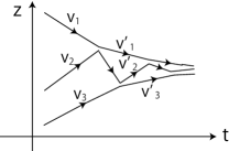
Figure 2: Schematic diagram for particle motion in the three body inelastic collapse in the one dimensional free space.

McNamara and Young McNamaraYoung-1992 have shown that the three-body inelastic collapse can occur if $e<e_{c}(3)\equiv 7-4\sqrt{3}$, by using the $3\times 3$ matrix $\cal{M}$ that relates the final velocities $\bm{v}^{\prime}=(v^{\prime}_{1},v^{\prime}_{2},v^{\prime}_{3})$ of the three particles after two successive collisions with their initial velocities $\bm{v}=(v_{1},v_{2},v_{3})$ as $\bm{v}^{\prime}={\cal M}\bm{v}$.

For $N=4$, the critical value can be evaluated as $e_{c}(4)=e_{c}^{\rm wall}(2)$ because of the symmetry in the order of collisions. If such symmetry in the order of collision process is assumed for $N>4$, one may obtain the relation

$$e_{c}(2N)=e_{c}^{\rm wall}(N),$$ (13)

but numerical simulations have shown that the relation Eq. (13) is not valid for large $N$ McNamara-2002 .

II.4 Asymptotic analysis for $N=3$

In this subsection, we examine the asymptotic behavior of the total number of collisions $n_{\rm tot}$ in a single collapsing event in the hard-sphere limit for the cases of $N=3$ and show that $n_{\rm tot}\sim\log k$ in the $k\to\infty$ limit.

The system with $N=3$ is the smallest one where the inelastic collapse can occur, since the floor provides a thermal drive, thus the inelastic collapse can happen only in sequence of collisions among particles. Then, we can argue the behavior of $n_{\rm tot}$ by considering a collision process of the three-body inelastic collapse in the hard-sphere limit as shown in Fig. 2. In this case, the time between the $(n-1)$th collision and $n$th collision, $t_{12}^{(n)}$, between the same pair of particles, say 1 and 2, behaves as

$$t_{12}^{(n)}\approx qt_{12}^{(n-1)}\approx q^{n}t_{12}^{(0)},$$ (14)

where $q$ is a constant smaller than unity (See Appendix A).

Now, let us discuss the case of the soft spheres with a finite $k$ and $e<e_{c}(3)$. In this case, initial binary collisions can follow a sequence similar to the inelastic collapse, but eventually all of the three particles are in contact after a finite number of collisions, and then fly away from each other with very small relative velocities. We estimate the total number $n_{\rm tot}$ of collisions before all three particles are in contact at the same time. Similar estimation has been done for the case of a single inelastic soft sphere bouncing on a floor to show $n_{\rm tot}\sim\log k$ as $k\to\infty$ MitaraiNakanishi-2003 . The three-body collapse like collision process shows essentially the same behavior as we will show in the following.

First of all, the collision interval $t_{12}^{(n)}$ for the case of the soft-sphere system is given by

$$t_{12}^{(n)} \approx qt_{12}^{(n-1)}+\Delta t_{12},$$ (15)

with the correction term $\Delta t_{12}$ in comparison with Eq. (14) because the collision duration $\tau_{c}$ is finite. It can be shown (see Appendix B) that

$$\Delta t_{12}=-f\tau_{c},$$ (16)

where $f$ is positive and a function of $e$. Substituting Eq. (16) into Eq. (15), we obtain

$$t_{12}^{(n)} \approx qt_{12}^{(n-1)}-f\tau_{c}$$ (17)

$$\approx q^{n}t_{12}^{(0)}-\sum_{i=0}^{n-1}q^{i}f\tau_{c}$$

$$= q^{n}t_{12}^{(0)}-\frac{1-q^{n}}{1-q}f\tau_{c}$$

The number of collisions $n_{\rm tot}$ before all three particles are in contact at the same time is given by the smallest $n$ that satisfies the condition $t_{12}^{(n+1)}\leq 2\tau_{c}$, because two successive collisions between particles 1 and 2 cannot be shorter than the twice of the duration time. Thus, by requiring the relation

$$t_{12}^{(n_{\rm tot})}\simeq 2\tau_{c},$$ (18)

for $n_{\rm tot}\gg 1$ and substituting Eq. (17), we obtain

$$q^{n_{\rm tot}}t_{12}^{(0)}\approx\left(2+\frac{1-q^{n_{\rm tot}}}{1-q}f\right)\tau_{c}.$$ (19)

$n_{\rm tot}$ diverges and $q^{n_{\rm tot}}$ goes to zero in the limit $k\to\infty$ because $\tau_{c}\propto k^{-1/2}$ and $0\leq q<1$. Thus, Eq. (19) can be written as $q^{n_{\rm tot}}t_{12}^{(0)}\sim ak^{-1/2}$, where $a$ is a coefficient that depends on $e$. Therefore, we obtain $n_{\rm tot}$

$$n_{\rm tot}\sim-\frac{1}{2\log q}\log k+\mbox{const.}$$ (20)

If we assume that the frequency $r$ of such a three-body process is independent of $k$, the collision rate is $n_{\rm coll}\sim r\,n_{\rm tot}$ and thus $n_{\rm coll}\sim\log k$ in the hard-sphere limit.

III Simulation results

The main quantity studied in this paper is the collision rate per particle $n_{\rm coll}$ defined as the average number of collisions (including collisions with the floor) per particle per unit time for various values of parameters, $k$, $e$, $N$ and $T_{0}$. We carried out numerical simulations to investigate $n_{\rm coll}$ in the hard-sphere limit. After describing simulation procedure, we present the results for small number of particles $3\leq N\leq 6$ first, and then for large number of particles $N\gtrsim 20$. We find qualitative difference between the two cases.

III.1 Simulation procedure

Numerical simulations are performed using the second-order Runge-Kutta method with the time step $dt=\tau_{\rm c}/100$, where $\tau_{\rm c}$ is the duration time of binary collision given by Eq.(6). All particles are initially placed in such a way that there is no overlap between particles and velocities are given randomly. After waiting for a sufficiently long time for the system to go through an initial transient, we start taking data for various quantities and their time average.

For numerical data, we employ the unit system where the particle mass $m$, the diameter $d$, and the gravitational acceleration $g$ are unities,

$$m=d=g=1.$$ (21)

We set temperature of the thermal floor $k_{\rm B}T_{0}=1$ unless otherwise stated. For a given set of $N$ and $e$, we measure the collision rate $n_{\rm coll}$ for $k=10^{5},\,10^{6},\,10^{7},\,10^{8},\,10^{9}$, and $10^{10}$.

Each collision event between two particles or between a particle and the floor is defined by their contact. The collisions between particles last for some duration time and they are counted everytime colliding particles separate, while the collisions with the floor are assumed to be instantaneous. The total number of collisions $N_{\rm coll}$ includes the collisions between particles and those between a particle and the floor, and the collision rate per particle $n_{\rm coll}$ is defined by

$$n_{\rm coll}=N_{\rm coll}/(NT),$$ (22)

where $T$ is the simulation time length. We set $T=10^{4}$ for $N<50$ and $T=10^{3}$ for $N\geq 50$.

III.2 Small systems

Let us first consider systems with small number of particles, in which a series of collisions occurs in a simple manner. Figure 3 shows the collision rates per particles, $n_{\rm coll}$ as a function of $k$ for various values of $e$ on the system with $N=3\sim 6$. For the system of $N=3$ (Fig. 3), the logarithmic behavior of $n_{coll}$ is clearly observed for $e<e_{c}(3)=7-4\sqrt{3}$, as has been suggested from the analysis in Sec. IID. On the other hand, for $e>e_{c}(3)$, $n_{\rm coll}$ converges to a finite value as $k$ becomes large. It should be noted, however, that $n_{\rm coll}$ increases faster than $\log k$ for $e=0.0718\simeq e_{c}(3)$.

For the systems with $N=$4, 5, and 6, such a region where $n_{\rm coll}$ increases faster than $\log k$ extends toward the smaller $e$ region than $e_{c}(N)$, $e<e_{c}(N)$, as is seen in Fig. 3. Here, $e_{c}(N)$ represents the critical restitution coefficient of the inelastic collapse for the free $N$ particle system evaluated by the ICW model with Eq. (9) and Eq. (13),

$$e_{c}(N)=\tan^{2}\left(\frac{\pi}{4}\left(1-\frac{2}{N}\right)\right),$$ (23)

which we expect accurate for small $N$.

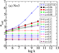
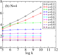
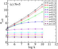
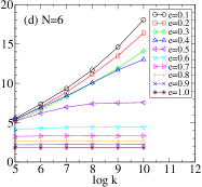
Figure 3: Collision rate per particle $n_{\rm coll}$ vs. $\log k$ for various values of the restitution coefficient $e$ for the systems with $N=3$ (a), 4 (b), 5 (c), and 6 (d).

In Fig. 4, $n_{\rm coll}$ is shown as a function of $e$ for $k=10^{5}\sim 10^{10}$ on the system with $N=3\sim 6$. One may notice that the curves have irregular-looking fine structures. We confirmed, however, that their statistical errors are small enough and that these fine structures are reproducible if we change sequences of random numbers in the simulations. Some of larger structures coincide with the critical restitution constants $e_{c}(n)$ with ($n=3,\cdots,N+1$), which are shown by the vertical dotted lines in Fig. 4. In the case of $N=3$ (Fig. 4), one can observe a sharp peak at $e_{c}(3)$, and the peak value of $n_{\rm coll}$ increases faster than $\log k$ as $k$ increases. For $e<e_{c}(3)$, $n_{\rm coll}$ increases by a nearly constant when $k$ becomes 10 times larger, which suggests that $n_{\rm coll}$ increases logarithmically as is discussed above.

For $N=3\sim 6$, there are a couple of features in common. First, a sharp peak appears at $e_{c}(n)(n=3,\cdots,N-1)$ and the peak at $e_{c}(3)$ is highest. Secondly, a dip appears at $e$ slightly larger than $e_{c}(N)$. Our simulation results (not shown here) suggest that this dip still exists for $N=10$, becomes unclear for $N=25$, and completely disappears for $N=30$.

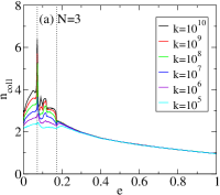
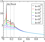
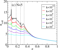
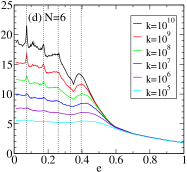
Figure 4: Collision rate per particle $n_{\rm coll}$ vs. $e$, plotted for $k=10^{5}\sim 10^{10}$ for the systems with $N=3$ (a), 4 (b), 5 (c), and 6 (d). The vertical dotted lines are at the restitution coefficient of $e_{c}(3)$, $e_{c}(4)$, $\cdots$, $e_{c}(N+1)$ from left to right.

III.3 Large systems

III.3.1 Collision rate in the large $k$ limit

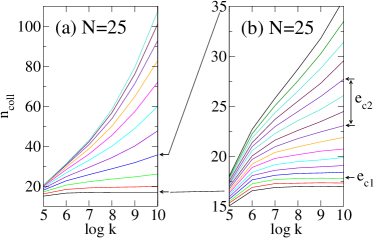
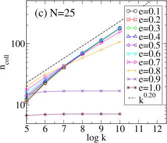
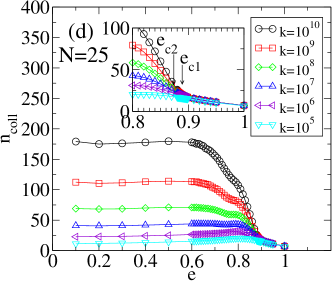
Figure 5: Collision rate per particle $n_{\rm coll}$ for $N=25$. $n_{\rm coll}-\log k$ is plotted for (a) $e=0.80\sim 0.90$ with an increment 0.01 from top to bottom. (b) $e=0.87\sim 0.90$ with an increment 0.002 from top to bottom. $\log n_{\rm coll}-\log k$ is plotted for (c) $e=0.1\sim 1.0$ with an increment 0.1. (d) $n_{\rm coll}-e$ is plotted for $k=10^{5}\sim 10^{10}$ from bottom to top with the inset that shows in close-up near the critical values $e_{c1}\approx 0.894$ and $e_{c2}\approx 0.88$.

For large systems, the power-law divergence of the collision rate dominates, but we can see clearly that there exists the region of restitution coefficient where $n_{\rm coll}$ diverges definitely slower than the power law.

In Fig. 5, we plot $n_{\rm coll}$ for $N=25$ as a function of $k$ for various values of $e$ (a, b, and c), and as a function of $e$ for various values of $k$ (d). It is clear in the logarithmic plot of Fig. 5(c) that $n_{\rm coll}$ converges for $e\gtrsim 0.9$ and diverges in the power-law for $e\lesssim 0.8$. The exponent $\alpha$ in the power-law regime depends on $e$, but is nearly constant $\alpha\simeq 0.2$ for $e\lesssim 0.6$ as can be seen from Fig. 5(c). In Fig. 5(d), we also observed that the value of $n_{\rm coll}$ itself is nearly independent of $e$ for any value of $k$ for $e\lesssim 0.6$, where the exponent $\alpha$ is nearly constant.

In the following, we will examine the transition region between the converging regime to the diverging regime carefully. Let us denote the lower limit of the restitution of the converging region by $e_{c1}$ and the upper limit of the power-law diverging region by $e_{c2}$. A close look at the region $0.8<e<0.9$ in the semi-logarithmic plots of Fig. 5(a, b) reveals that there are two regimes within the region where $n_{\rm coll}$ diverges: the convex regime and the concave regime as a function of $\log k$. In the convex regime, $n_{\rm coll}$ diverges faster than $\log k$, suggesting that it is a part of the power-law regime. In the concave regime, the divergence is slower and it seems that $n_{\rm coll}$ eventually shows the logarithmic divergence

$$n_{\rm coll}\sim b(e,N)\log k+\mbox{const.}$$ (24)

in the large $k$ limit with the coefficient $b$ that depends on $e$ and also on $N$. The lower limit of the converging regime $e_{c1}$ is determined as the upper limit of the divergence; the data are fitted to Eq.(24) in the asymptotic region, then $e_{c1}$ is the point where $b=0$. On the other hand, the value of $e_{c2}$ is estimated by the boundary between the convex and the concave regime. By these procedures, we obtain that $e_{c1}\simeq 0.894$ and $e_{c2}$ is somewhere between 0.878 and 0.884 for $N=25$. The values of $e_{c1}$ and $e_{c2}$ are determined for several values of $N$, and plotted with error bars in the $1/N$-$(1-e)$ plane in Fig. 6. One can see that they fit very well to the lines

$$(1-e_{c1}^{\rm fit})={2.6\over N},\quad(1-e_{c2}^{\rm fit})={3.0\over N}.$$ (25)

Note that their functional form is the same with the asymptotic form of $e_{c,{\rm ICW}}^{\rm wall}$ in Eq. (11).

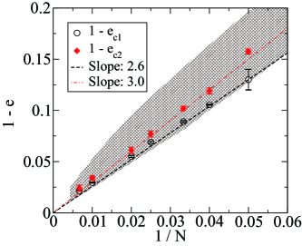
Figure 6: Bifurcation diagram for the three regimes. The critical values of $e_{c1}$ and $e_{c2}$ are plotted for $N=$20, 25, 30, 40, 50, 100, and 150. The error bars show ambiguity of the results in the procedure. The dashed and the dashed dotted lines show the fitting lines for $e_{c1}$ and $e_{c2}$ by $(1-e_{c1}^{\rm fit})={2.6/N}$ and $(1-e_{c2}^{\rm fit})={3.0/N}$, respectively. The shaded region represents the region where the partially condensed state appears; its boundary is estimated at $N=$20, 25, 30, 50, 100 and 150.

We further examine $b(e,N)$ in Eq.(24) as a function of both $e$ and $N$ by simulation data. From Eq.(25), we expect that $b(e,N)$ is expressed by a simple function of $(1-e)-A/N$ with a constant $A\approx 2.6$. This is actually what we find in Fig. 7(a), where we plot $b(e,N)/N^{5/2}$ against $(1-e)-2.6/N$ for various values of $N$ and $e$ in the logarithmic scale. One can see that the data collapse on a straight line with the slope 2, which means

$$b(e,N)\sim N^{5/2}\Bigl{(}(1-e)-2.6/N\Bigr{)}^{2},$$ (26)

from which we confirm the asymptotic form

$$e_{c1}\simeq 1-{2.6\over N}.$$ (27)

It should be noted that this result is very close to the critical values of $e$ below which clustering starts in the 1-d granular system driven by a vibrating bottom plate, i.e. $e_{c}\approx 1-2.5/N$ LudingClementBlumenRajchenbachDuran-1994 and $e_{c}\approx 1-2.6/N$ BernuDelyonMazighi-1994 .

Based upon above analysis, we conclude that the critical values, $e_{c1}$ and $e_{c2}$, do not coincide; therefore, in addition to the converging regime, there are two diverging regimes in $e$ with respect to behavior of $n_{\rm coll}$ in the hard-sphere limit $k\to\infty$: (i) uncollapsing regime, $e>e_{c1}$, where $n_{\rm coll}$ converges to a constant value, (ii) logarithmically collapsing regime, $e_{c1}>e>e_{c2}$, where $n_{\rm coll}$ diverges as $n_{\rm coll}\sim\log k$, and (iii) power-law collapsing regime, $e<e_{c2}$, where $n_{\rm coll}$ diverges as $n_{\rm coll}\sim k^{\alpha}$.

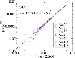
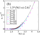
Figure 7: (a) $b(e,N)/N^{5/2}$ vs. $(1-e)-2.6/N$ in the logarithmic scale. $b(e,N)$ is defined in Eq.(24) and estimated from the plots similar to those in Fig.5(c) for various values of $N$ and $e$ in the logarithmically collapsing regime. The dashed line gives a fit by $1.5((1-e)-2.6/N)^{2}$ for $b/N^{5/2}$. (b) $b(e,N)/N^{1/2}$ vs. $N(1-e)$ in the linear scale using the same data as in (a). The range of values of $e$ used to plot (a) and (b) is the following: $0.835\leq e\leq 0.900$ for $N=20$, $0.876\leq e\leq 0.900$ for $N=25$, $0.894\leq e\leq 0.920$ for $N=30$, $0.918\leq e\leq 0.940$ for $N=40$, $0.932\leq e\leq 0.960$ for $N=50$, $0.963\leq e\leq 0.972$ for $N=100$, and $0.972\leq e\leq 0.979$ for $N=150$.

III.3.2 Partially condensed state

We observe a partial condensation near the bottom around a certain value of $e$. Figure 8 shows the spatial variation of the positional fluctuation (a) and the kinetic energy (b) of each particle for various values of $e$ for $N=25$; Fig. 8 shows the standard deviation $\sigma_{i}$ of the position of the particle $i$ divided by the one $\sigma_{0\,i}$ for the elastic case $e=1$, and (b) shows the kinetic energy $K_{i}$ of the particle $i$. Note that $K_{i}=(1/2)k_{\rm B}T_{0}$ for any particle when $e=1$.

For $e\gtrsim 0.91$, $\sigma_{i}/\sigma_{i\,0}$ and $K_{i}$ are larger in the region closer to the bottom and they decrease monotonically as the particle index $i$ increases. This is because the thermal wall at the bottom supplies the kinetic energy to the bottom particle, and the kinetic energy is dissipated as it is transported away from the bottom via the inelastic collisions. However, around $e\simeq 0.9$, a dip appears near the bottom both in $\sigma_{i}/\sigma_{0\,i}$ and $K_{i}$, and there appears the inversion layer where the temperature increases with $i$. This means that the low temperature and high density domain appears near the bottom. We call this the partially condensed state. For $N=25$, the value of $e\simeq 0.9$ where the partially condensed state appears almost coincides with, but seems to be slightly larger than $e_{c1}\simeq 0.894$, i.e. the critical point of the inelastic collapse.

The condensed domain with low $\sigma_{i}/\sigma_{i\,0}$ in Fig. 8 extends towards the upper part of the system as $e$ is decreased down to $0.84$, where the whole system is condensed. That is, the partially condensed state appears for $0.84\lesssim e\lesssim 0.90$, namely, the partially condensed state appears both in the logarithmically collapsing and the power-law collapsing regimes.

In Figure 6, the region for the partially condensed state is shown by the shaded area in the $1/N$-$(1-e)$ plane. One can see that the upper bound of $e$ (the lower boundary in Fig. 6) for the partially condensed state nearly coincides with $e_{c1}$ for all of the cases examined.

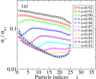
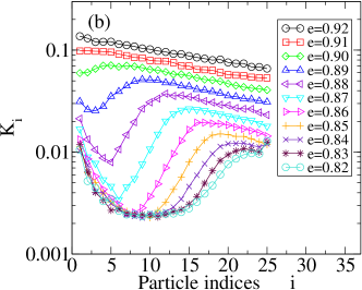
Figure 8: Spatial variation of the particle fluctuation of position and the kinetic energy for $e=0.82\sim 0.92$ for the system with $N=25$. (a) The standard deviation of particle position $\sigma_{i}$ of particle $i$, normalized by the corresponding value for $e=1$, $\sigma_{0,i}$. (b) The kinetic energy $K_{i}$ of the particle $i$. The data are shown for the cases with the elastic constant $k=10^{10}$.

III.3.3 Exponent in the power-law collapsing regime

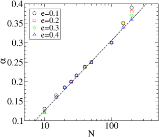
Figure 9: Exponent of the power law $\alpha$ for $e=0.1,\,0.2,\,0.3,$ and $0.4$ plotted as a function of $N$. The dashed line gives a fit by $0.18\log N-0.054$.

We observed that $n_{\rm coll}$ is almost constant when $e\leq 0.4$ for $N=25$ as can be seen in Fig 5. We examined this for the case with $N=20\sim 150$, and found this is true for all the cases. In Fig. 9, the exponents $\alpha$ for $e=$0.1, 0.2, 0.3 and 0.4 are plotted against $\log N$. One can see that $\alpha$ does not change by $e$ but depends linearly on $\log N$ and can be fitted to

$$\alpha^{\rm fit}=0.18\log N-0.054\simeq 0.18\log\left(N/2\right).$$ (28)

This logarithmic dependence of the exponent $\alpha$ on $N$ means that $n_{\rm coll}$ is given by

$$n_{\rm coll}\sim(N/2)^{0.18\log k},$$ (29)

for $e\leq 0.4$.

III.3.4 Effect of the floor temperature $T_{0}$

We find no qualitative difference in the $k$-dependence of $n_{\rm coll}$ by changing $k_{\rm B}T_{0}$ from 1 to 10 in both systems with $N=25$ and $50$. We show in Table 1 the critical values $e_{c1}$ and $e_{c2}$, and the average exponent of the power law $\overline{\alpha}$ for $k_{\rm B}T_{0}=1$ (see Sec. IIIC.1), $2$, $4$, and $10$ for the systems with $N=25$ and $50$. Here $\overline{\alpha}$ is the arithmetic mean of the four values of $\alpha$ at $e=0.1,\,0.2,\,0.3,$ and $0.4$, for which $\alpha$’s are almost constant independent of $e$. The both critical values and the power law exponent seem to be independent of $T_{0}$.

00$N$	00$k_{\rm B}T_{0}$00	00$e_{c1}$00	00$e_{c2}$00	0000000$\overline{\alpha}$00000
0025	$1$	$0.894$	00$0.878\sim 0.884$	000.20
	$2$	$0.892$	00$0.874\sim 0.880$	000.20
	$4$	$0.892$	00$0.872\sim 0.880$	000.20
	$10$	$0.890$	00$0.872\sim 0.878$	000.19
0050	$1$	$0.944$	00$0.942\sim 0.936$	000.25
	$2$	$0.944$	00$0.938\sim 0.942$	000.25
	$4$	$0.944$	00$0.938\sim 0.940$	000.24
	$10$	$0.944$	00$0.934\sim 0.944$	000.24

Table 1: The critical values $e_{c1}$, $e_{c2}$ and the average exponent of the power law $\overline{\alpha}$ for various values of the floor temperature $T_{0}$ for the systems with $N=25$ and $50$. The average exponent $\overline{\alpha}$ is defined as the arithmetic mean of the four values of $\alpha$ at $e=0.1,\,0.2,\,0.3,$ and $0.4$.

III.4 Inelastic collapse in the free space

In order to narrow down the possible origin of the power law divergence of the collision rate, we further simplify the system and consider the $N$-particle system in the 1-d free space without the external drive and the gravity. We performed MD simulations to see how the total number of collisions behaves in the hard sphere limit.

In the initial state, $N$ particles of the diameter $d$ are placed at an equal interval with the space $a$,

$$x_{i}=\left(i-{N+1\over 2}\right)(d+a);\quad i=1,2,\cdots N,$$ (30)

with the initial velocities,

$$v_{i}=-v_{0}\,{\rm sgn}(x_{i})+\delta v_{0}\,\xi_{i},$$ (31)

where ${\rm sgn}(x)$ is the sign function and $\xi_{i}$’s are random numbers distributed uniformly over the interval $[-1,1)$; $v_{0}$ and $\delta v_{0}$ are positive parameters.

We count the total number of collisions $n_{\rm tot}$ until the relative velocity of the end particles $v_{N}-v_{1}$ becomes positive. The results are shown in Fig.10 for the systems with $N=3$ (a) and 25 (b) for $d=a=v_{0}=1$ and $\delta v_{0}=0.1$. One can see that the total number of collisions $n_{\rm tot}$ behaves in an analogous way with the collision rate $n_{\rm coll}$ in the driven system under the gravity shown in Figs.3 and 5(c). For the case of $N=3$, $n_{\rm tot}$ converges to a finite value when $e>e_{c}(3)\simeq 0.0718$ and diverges as $\log k$ when $e<e_{c}(3)$. The dashed lines in Fig.10 show Eq.(20) with $q$ given by Eq.(49) for the corresponding $e$ values, and adjusted constants. As for the case of $N=25$, $n_{\rm tot}$ diverges as $k^{\alpha}$ when $e\lesssim 0.6$ with the exponent close to the value $\alpha\simeq 0.2$ for the previous case with the drive and the gravity.

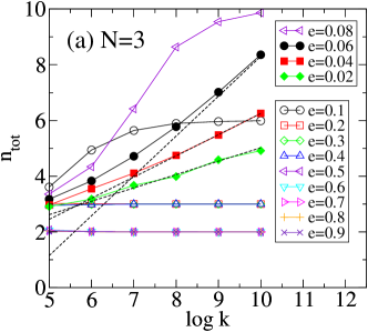
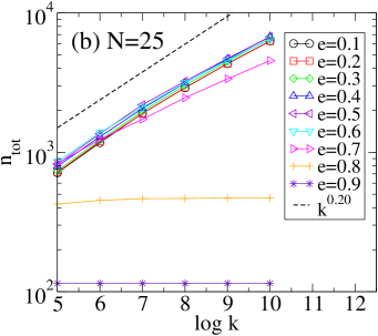
Figure 10: $n_{\rm tot}$ vs. $\log k$ for various values of $e$ (a) for $N=3$ in the log-linear scale and (b) for $N=25$ in the log-log scale. The parameters for the initial state are $a=v_{0}=1$ and $\delta v_{0}=0.1$. Each data point represents an average over $1000$ realizations by different random number $\xi_{i}$’s. The dashed lines in (a) show the asymptotic behavior given by Eq.(20) with $q$ given by Eq.(49) for the corresponding $e$ values after the constants being adjusted to the data. The dashed line in (b) is the line with the slope 0.2.

IV Summary and Discussions

We have studied the inelastic collapse in the 1-d system under the gravity with the random driving from the bottom floor. Using MD simulations for the soft-sphere systems, we calculated the collision rate per particle $n_{\rm coll}$ and see how it diverges/converges in the hard-sphere limit; The hard-sphere limit is taken by the infinite limit of the elastic constant, $k\to\infty$ with the restitution coefficient $e$ being kept constant. We have found that there are three regimes in the restitution coefficient $e$: (i) the uncollapsing regime for $1\geq e>e_{c1}$, where $n_{\rm coll}$ converges, (ii) the logarithmically collapsing regime for $e_{c1}>e>e_{c2}$, where $n_{\rm coll}$ diverges as $n_{\rm coll}\sim\log k$, and (iii) the power-law collapsing regime for $e_{c2}>e>0$, where $n_{\rm coll}\sim k^{\alpha}$. For small $N$ systems, the region of $e$ for the power-law collapsing regime is small and disappears for $N=3$. On the other hand, for large $N$ systems, the region for the power-law collapsing regime expands in the way that both of $e_{c1}$ and $e_{c2}$ approaches 1 as Eq.(25). As for the floor temperature effect, we have checked the critical restitution constants $e_{c1}$ and $e_{c2}$ and the power law exponent $\alpha$ for the system of $N=25$ and $50$, and found virtually no change for all of them in the temperature range of $1\leq k_{\rm B}T_{0}\leq 10$.

If the intervals of collisions follow a geometrical sequence toward the inelastic collapse, the logarithmic divergence of the collision number can be understood based on the consideration that the collision sequence terminates at the point where the collision interval becomes comparable with the duration time of binary collision. In the case of one particle bouncing on a floor under the gravity, it is obvious that the collision times follow the geometrical sequence. We have shown that it holds also for the three-particle system in the 1-d free space. Thus, the logarithmic divergence of the collision rate for the externally driven system can be understood if the inelastic collapses occur at a certain rate and they do not interfere each other nor are affected by the external drive in the hard-sphere limit, $k\to\infty$.

On the other hand, the power-law divergence of the collision rate is more intriguing. It has been reported in the gravitational slope flows MitaraiNakanishi-2003 , but our results show that it occurs in an even simpler system, i.e. a 1-d externally driven system under the gravity. If we try to understand this in the same way as above, the collision interval should decrease as a power of collision number. This possibility is supported by the fact that the total number of collisions in the free space also diverges in the power law in the hard sphere limit. If this is true, we still need to understand how the power law sequence collision intervals arises.

For the small $N$ systems, the collision rate shows a certain structure as a function of $e$ at $e=e_{c}(n)$ of $3\leq n\leq N+1$, i.e. the critical restitution coefficient for the $n$-particle system in the free space. For $N=3$, there is a sharp peak at $e=e_{c}(3)$ and a dip at $e=e_{c}(4)$, while for $3<N\leq 6$, we find peaks at $e=e_{c}(n)$ for $3\leq n\leq N-1$, a dip or a shoulder at $e\simeq e_{c}(N)$, and a somewhat broad peak around $e\simeq e_{c}(N+1)$. Such a structure becomes vague for larger $N$. Note that the relative motion of $n$ particles under gravity with respect to their center of mass is equivalent to the motion in the free space as long as they do not interact with their surrounding particles. Thus, the structure at $e_{c}(n)$ for $n<N$ should be an effect of the inelastic collapse in which a part of the system is involved, but we do not understand yet how it shows up as a sharp peak or a dip structure, depending on the number of particles involved.

For large $N$, it is also intriguing that the collision rate is independent of $e$ for a rather wide range; In the case of $N=25$, $n_{\rm coll}$ is constant in the region $e\lesssim 0.6$ for any $k$, thus the exponent $\alpha$ also does not depend on $e$ in the same region. Within the range $20\leq N\leq 150$, $n_{\rm coll}$ is almost constant for $e\leq 0.4$, but the power-law exponent increases depending linearly on $\log N$ as $N$ is increased.

One may find that some data points for $N>100$ in Figs. 6, 7(b), and 9 seem to deviate systematically from the asymptotic fitting expressions given by Eqs. (25), (26), and (28), respectively. This may be due to the excessive load on particles near the floor. In the case of very large $N$, the load on the particles near the floor becomes so large that the contacts among them cannot be resolved into binary collisions but may remain as a long-lived contacts in the range of $k$ investigated. In such a case, the system behavior may deviate from the assumed asymptotic forms.

It is found that there appears the partially condensed state, where some particles near the bottom condense with lower kinetic energy. The region where the partially condensed state appears in the $N$-$(1-e)$ plane covers the logarithmically collapsing regime; It starts hardly inside the uncollapsing regime and extends somewhat into the power-law collapsing regime. The condensed state near $e_{c1}$ contains only a few particles, but the number of condensed particles increases as $e$ decreases. The fact that the partially condensed state starts almost at $e_{c1}$ suggests that the inelastic collapse causes the condensation, but it remains to be understood how a small number of particles can condense by the inelastic collapse at $e\approx e_{c1}$, that is much larger than $e_{c}(n)$ for small $n$.

The partially condensed state has already been observed in the 1-d granular systems driven by a vibrating bottom plate in various forms of vibration. In the case of the sinusoidal vibration, the condensed state has been shown to appear for $N(1-e)\gtrsim 2.5$ LudingClementBlumenRajchenbachDuran-1994 , and in the cases of a sawtooth vibration and a piecewise quadratic vibration, for $N(1-e)\gtrsim 2.6$ BernuDelyonMazighi-1994 . Our result shows that the partially condensed state appears below $e_{c1}$, which means $N(1-e)\gtrsim 2.6$ from Eq. (27). These results are consistent with each other and show that the point where the system starts to condense is not sensitive to the driving mode.

In summary, we have demonstrated that the inelastic collapse shows up in the 1-d driven system under the gravity as the diverging collision rate in the large $k$ limit with keeping the restitution coefficient $e$ constant. By numerical simulations, we found that there are three regimes for the way that the collision rate diverges, i.e. the uncollapsing regime, the logarithmically collapsing regime, and the power-law collapsing regime.

Appendix A

In this appendix, we consider the three-body inelastic collapse of the inelastic hard spheres in the free space and derive the asymptotic behavior Eq. (14) of the time $t_{12}^{(n)}$ between two successive collisions between the particles 1 and 2.

Let $t^{(n)}$ be the time of the $n$th collision between the particles 2 and 3 and $t^{\prime(n)}$ be the time of the $n$th collision between the particles 1 and 2, and define $t_{1}^{(n)}={t^{\prime}}^{(n)}-t^{(n)}$ and ${t}_{2}^{(n)}=t^{(n+1)}-t^{\prime(n)}$ (See, Fig. 11). Similarly, the particle velocities just after $t^{(n)}$ are $v_{i}^{(n)}\,(i=1,2,3)$, those just after ${t^{\prime}}^{(n)}$ are ${v^{\prime}}_{i}^{(n)}\,(i=1,2,3)$. The relative velocities are denoted by $v_{21}^{(n)}=v_{2}^{(n)}-v_{1}^{(n)}$ and $v_{32}^{(n)}=v_{3}^{(n)}-v_{2}^{(n)}$. The separation between the particles 1 and 2 at $t^{(n)}$ is denoted by $x_{21}^{(n)}$ and that between the particles 2 and 3 at ${t^{\prime}}^{(n)}$ by ${x^{\prime}}_{32}^{(n)}$.

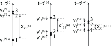
Figure 11: Schematic picture of collision sequence occurring in the three-body inelastic collapse in the free space.

The time $t_{1}^{(n)}$ and $t_{2}^{(n)}$ are then written as

$$t^{(n)}_{1} = \frac{x^{(n)}_{21}}{|v^{(n)}_{21}|},\hskip 28.45274pt{t}^{(n)}_{2}=\frac{{x^{\prime}}^{(n)}_{32}}{|{v^{\prime}}^{(n)}_{32}|},$$ (32)

respectively. The separations $x_{21}^{(n)}$ and ${x^{\prime}}_{32}^{(n)}$ can also be expressed as

$$x^{(n)}_{21}={v^{\prime}}^{(n-1)}_{21}{t}^{(n-1)}_{2},\hskip 28.45274pt{x^{\prime}}^{(n)}_{32}=v^{(n)}_{32}t^{(n)}_{1},$$ (33)

respectively. Combining Eqs. (32) and (33), we can write

$$t^{(n)}_{1} = \frac{{v^{\prime}}^{(n-1)}_{21}}{|v^{(n)}_{21}|}\cdot\frac{v^{(n-1)}_{32}}{|{v^{\prime}}^{(n-1)}_{32}|}\,t^{(n-1)}_{1}$$ (34)

Using $v^{(n-1)}_{21}=-\frac{1}{e}{v^{\prime}}^{(n-1)}_{21}$ and $v^{(n)}_{32}=-e{v^{\prime}}^{(n-1)}_{32}$, we can further rewrite it as

$$t^{(n)}_{1} = \frac{1}{e^{2}}\frac{{v}^{(n)}_{32}}{|v^{(n)}_{21}|}\cdot\frac{{v}^{(n-1)}_{32}}{|v^{(n-1)}_{21}|}\left(\frac{v^{\prime(n-1)}_{21}}{|{v^{\prime}}^{(n-1)}_{32}|}\right)^{2}t^{(n-1)}_{1}.$$ (35)

This relation can be expressed using the ratio of the relative velocities $m^{(n)}=v^{(n)}_{32}/v^{(n)}_{21}$ and ${m^{\prime}}^{(n)}={v^{\prime}}^{(n)}_{32}/{v^{\prime}}^{(n)}_{21}$ as

$$t^{(n)}_{1} = \frac{1}{e^{2}}\frac{m^{(n)}m^{(n-1)}}{({m^{\prime}}^{(n-1)})^{2}}\,t^{(n-1)}_{1}.$$ (36)

The sequence of $m^{(n)}$ and ${m^{\prime}}^{(n)}$, which are completely determined by the collision laws and the initial condition $m^{(0)}$ (or ${m^{\prime}}^{(n)}$), has been studied by Constantin et al. ConstantinGrossmanMungan-1995 . We briefly summarize their results that are relevant for our purpose in this appendix. Upon a collision between particles 1 and 2, velocities after the collision $(v^{\prime}_{1},v^{\prime}_{2})$ and before the collision $(v_{1},v_{2})$ are related by

$$\left(\begin{array}[]{c}v^{\prime}_{1}\\ v^{\prime}_{2}\end{array}\right) = \left(\begin{array}[]{cc}\frac{1-e}{2}&\frac{1+e}{2}\\ \frac{1+e}{2}&\frac{1-e}{2}\end{array}\right)\left(\begin{array}[]{c}v_{1}\\ v_{2}\end{array}\right).$$ (43)

From this collision law, we can deduce the following relations:

$${m}^{(n)} = -e\frac{{m^{\prime}}^{(n-1)}}{1+b\,{m^{\prime}}^{(n-1)}},$$ (44)

$${m^{\prime}}^{(n)} = -\frac{1}{e}\left(m^{(n)}+b\right),$$ (45)

where $b\equiv(1+e)/2$. If $e<e_{c}(3)=7-4\sqrt{3}$ and $m^{(0)}$ (or ${m^{\prime}}^{(0)}$) is such that the collision sequence continues infinitely, i.e. the inelastic collapse occurs, then $m^{(n)}$ and $m^{\prime(n)}$ should converge to the stable fixed point values

$$m^{*} = \frac{1}{2}\left(-b+\sqrt{b^{2}-4e}\right),$$ (46)

$${m^{\prime}}^{*} = \frac{1}{2e}\left(-b-\sqrt{b^{2}-4e}\right),$$ (47)

which are real when $e\leq e_{c}(3)$.

Therefore, if both $n$ and $n^{\prime}$ are so large that $m^{(n)}\approx m^{(n^{\prime})}\approx m^{*}$ and ${m^{\prime}}^{(n)}\approx{m^{\prime}}^{(n^{\prime})}\approx{m^{\prime}}^{*}$, Eq. (36) can be written as

$$t^{(n)}_{1}\approx\left(\frac{m^{*}}{e\,{m^{\prime}}^{*}}\right)^{2}t^{(n-1)}_{1}\approx\left(\frac{m^{*}}{e\,{m^{\prime}}^{*}}\right)^{2(n-n^{\prime})}t^{(n^{\prime})}_{1}.$$ (48)

It is straightforward to show

$$\left(\frac{m^{*}}{e\,{m^{\prime}}^{*}}\right)^{2}={1-6e+e^{2}-(1+e)\sqrt{1-14e+e^{2}}\over 1-6e+e^{2}+(1+e)\sqrt{1-14e+e^{2}}}\equiv q,$$ (49)

and $0\leq q<1$ for $0\leq e<e_{c}(3)$. If we start to count the number of collisions at $n^{\prime}$, namely we put $n^{\prime}=0$, then we have

$$t^{(n)}_{1}\approx q^{n}\,t^{(0)}_{1}.$$ (50)

Because of symmetry with regard to exchange of particles, ${t}^{(n)}_{2}$ should have the same property, and we finally obtain

$$t_{12}^{(n)}={t}^{(n)}_{1}+{t}^{(n-1)}_{2}\approx q^{n}\,t_{12}^{(0)},$$ (51)

which is Eq. (14).

Appendix B

In this appendix, we turn to the problem of the three-body inelastic collapse like collisions among the inelastic soft spheres and derive the asymptotic behavior Eqs. (15) and (16) of the time $t_{12}^{{\rm S}(n)}$ between the instants of the end of contact at two successive collisions between the soft particles 1 and 2. We put superscript ${\rm S}$ for quantities that are defined for soft particles in this appendix, in order to distinguish them from the corresponding quantities defined for hard particles in Appendix A.

Let $\tilde{t}^{{\rm S}(n)}$ and $t^{{\rm S}(n)}$ be the times of the beginning and the end of contact at the $n$th collision between the particles 2 and 3, respectively (See, Fig. 12). Similarly, let $\tilde{t^{\prime}}^{{\rm S}(n)}$ and ${t^{\prime}}^{{\rm S}(n)}$ be the times of the beginning and the end of contact at the $n$th collision between the particles 1 and 2. We define the time intervals during which the particles move freely as $t_{1}^{{\rm S}(n)}\equiv\tilde{t^{\prime}}^{{\rm S}(n)}-t^{{\rm S}(n)}$ and $t_{2}^{{\rm S}(n)}\equiv\tilde{t}^{{\rm S}(n+1)}-{t^{\prime}}^{{\rm S}(n)}$. Using the duration time $\tau_{c}$ of contact for a binary collision (see Eq. (6)), $t_{12}^{{\rm S}(n)}$ can be represented as

$$t_{12}^{{\rm S}(n)}=t_{1}^{{\rm S}(n)}+t_{2}^{{\rm S}(n-1)}+2\tau_{c},$$ (52)

because two collisions occur during the time $t_{12}^{{\rm S}(n)}$.

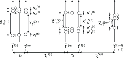
Figure 12: Schematic picture of collision sequence occurring in the three-body inelastic collapse like collisions among the inelastic soft spheres in the free space.

We denote the relative distance between the particles 1 and 2 just before the $n$th collision between the particles 2 and 3 as $\tilde{x}_{21}^{{\rm S}(n)}$, and that just after the collision as $x_{21}^{{\rm S}(n)}$. Similarly, the relative distance between the particles 2 and 3 just before the $n$th collision between the particles 1 and 2 is $\tilde{x^{\prime}}_{32}^{{\rm S}(n)}$, and that just after the collision is ${x^{\prime}}_{32}^{{\rm S}(n)}$. The relative distances just before and just after a collision are related as follows:

$$x_{21}^{{\rm S}(n)} = \tilde{x}_{21}^{{\rm S}(n)}+V_{1}^{(n)}\tau_{c},$$ (53)

$${x^{\prime}}_{32}^{{\rm S}(n)} = \tilde{x^{\prime}}_{32}^{{\rm S}(n)}+V_{3}^{(n)}\tau_{c},$$ (54)

where $V_{1}^{(n)}$ is the relative velocity of the center of mass of the particles 2 and 3 with respect to the particle 1, and $V_{3}^{(n)}$ is the relative velocity of the particle 3 with respect to the center of mass of the particles 1 and 2,

$$V_{1}^{(n)} \equiv \frac{v_{3}^{(n)}+v_{2}^{(n)}}{2}-v_{1}^{(n)}=v_{21}^{(n)}+\frac{1}{2}v_{32}^{(n)},$$ (55)

$$V_{3}^{(n)} \equiv v_{3}^{(n)}-\frac{v_{2}^{(n)}+v_{1}^{(n)}}{2}=v_{32}^{(n)}+\frac{1}{2}v_{21}^{(n)}.$$ (56)

The relation Eqs. (32) and (33) for the hard particles should be modified for the soft spheres as

$$t^{{\rm S}(n)}_{1} = \frac{x^{{\rm S}(n)}_{21}}{|v^{(n)}_{21}|},\hskip 28.45274ptt^{{\rm S}(n)}_{2}=\frac{{x^{\prime}}^{{\rm S}(n)}_{32}}{|{v^{\prime}}^{(n)}_{32}|},$$ (57)

and

$$\tilde{x}^{{\rm S}(n)}_{21} = {v^{\prime}}^{(n-1)}_{21}{t}^{{\rm S}(n-1)}_{2},\hskip 14.22636pt\tilde{x^{\prime}}^{{\rm S}(n)}_{32}=v^{(n)}_{32}t^{{\rm S}(n)}_{1},$$ (58)

respectively. Combining Eqs. (53), (54), (57) and (58), we can write

$$t_{1}^{{\rm S}(n)} = \frac{{v^{\prime}}_{21}^{(n-1)}}{|v_{21}^{(n)}|}\frac{v_{32}^{(n-1)}}{|{v^{\prime}}_{32}^{(n-1)}|}t_{1}^{{\rm S}(n-1)}$$ (59)

$$+ \frac{1}{|v_{21}^{(n)}|}\left[\frac{{v^{\prime}}_{21}^{(n-1)}}{|{v^{\prime}}_{32}^{(n-1)}|}V_{3}^{(n-1)}+V_{1}^{(n)}\right]\tau_{c}.$$

Substituting Eqs. (55) and (56) into Eq. (59) and using the ratio of the relative velocities $m^{(n)}$ and ${m^{\prime}}^{(n)}$ defined in Appendix A, $t_{1}^{{\rm S}(n)}+\tau_{c}$ can be expressed as

$$t_{1}^{{\rm S}(n)}+\tau_{c} = \frac{1}{e^{2}}\frac{m^{(n)}m^{(n-1)}}{({m^{\prime}}^{(n-1)})^{2}}\left(t_{1}^{{\rm S}(n-1)}+\tau_{c}\right)$$ (60)

$$+ \frac{1}{2}m^{(n)}\left[\frac{1}{(e{m^{\prime}}^{(n-1)})^{2}}-1\right]\tau_{c}.$$

Note that the sequence of the particle velocities $v_{i}^{(n)}(i=1,2,3)$ and that of $m^{(n)}$ and ${m^{\prime}}^{(n)}$ are completely determined by the collision laws and their initial conditions regardless whether the particles are hard or soft. Using the relations Eqs. (44) and (45) and the fact $m^{(n)},\,{m^{\prime}}^{(n)}<0$ in the collapse like collision processes, it can be shown that the second term on the right-hand side of Eq. (60) is negative.

If $m^{(n)}$ and ${m^{\prime}}^{(n)}$ converge sufficiently fast to their stable fixed point values $m^{*}$ and ${m^{\prime}}^{*}$, and we start to count the number of collisions after $m^{(n)}\approx m^{*}$ and ${m^{\prime}}^{(n)}\approx{m^{\prime}}^{*}$ are reached, we can write

$$t_{1}^{{\rm S}(n)}+\tau_{c}$$ (61)

$$\approx q\left(t_{1}^{{\rm S}(n-1)}+\tau_{c}\right)+\frac{m^{*}}{2}\left[\frac{1}{(e{m^{\prime}}^{*})^{2}}-1\right]\tau_{c},$$

for any $n\geq 1$.

Because of symmetry with regard to exchange of particles, $t_{2}^{{\rm S}(n)}$ should have the same expression as Eq. (61). Substituting Eq. (61) into Eq. (52), we finally obtain Eqs. (15) and (16):

$$t_{12}^{{\rm S}(n)}=qt_{12}^{{\rm S}(n-1)}-f\tau_{c},$$ (62)

where

$$f\equiv-m^{*}\left[\frac{1}{(e{m^{\prime}}^{*})^{2}}-1\right],$$ (63)

which is a positive function of $e$.

References

- (1) D. C. Rapaport, J. Comput. Phys. 34, 184 (1980).
- (2) S. Luding, in The Physics of Granular Media, edited by H. Hinrichsen and D. E. Wolf (Wiley-VCH, Weinheim, 2004), p.299.
- (3) M. Isobe, Int. J. Mod. Phys. C 10,1281 (1999).
- (4) N. V. Brilliantov and T. Pöschel, Kinetic Theory of Granular Gases (Oxford University Press, Oxford, 2004).
- (5) B. Bernu and R. Mazighi, J. Phys. A: Math. Gen. 23,5745 (1990).
- (6) S. McNamara and W. R. Young, Phys. Fluids A 4, 496 (1992).
- (7) S. McNamara and W. R. Young, Phys. Rev. E 50, R28, (1994).
- (8) S. McNamara and W. R. Young, Phys. Rev. E 53, 5089 (1996).
- (9) T. Zhou and L. P. Kadanoff, Phys. Rev. E 54, 623 (1996).
- (10) N. Schörghofer and T. Zhou, Phys. Rev. E 54, 5511 (1996).
- (11) M. Alam and C. M. Hrenya, Phys. Rev. E 63, 061308 (2001).
- (12) M. Jean and J. J. Moreau, in Proceedings of Contact Mechanics International Symposium, edited by A. Curnier (Presses Polytechniques et Universitaires Romandes, Lausanne, Switzerland, 1992), p. 31.
- (13) J. J. Moreau, Eur. J. Mech. A/Solids 13, 93 (1994).
- (14) D. Goldman, M. D. Shattuck, C. Bizon, W. D. McCormick, J. B. Swift, and H. L. Swinney, Phys. Rev. E 57, 4831 (1998).
- (15) C. Bizon, M. D. Shattuck, J. R. de Bruyn, J. B. Swift, W. D. McCormick, and H. L. Swinney, J. Stat. Phys. 93, 449 (1998).
- (16) W. Goldsmith, Impact: The Theory and Physical Behaviour of Colliding Solids, (Arnold, London, 1960).
- (17) A. Ferguson and B. Chakraborty, Phys. Rev. E 73, 011303 (2006).
- (18) G. Lois, A. Lemaître, and J. M. Carlson, Phys. Rev. E 76, 021302 (2007).
- (19) N. Mitarai and H. Nakanishi, Phys. Rev. E 67, 021301 (2003).
- (20) R. Brewster, L. E. Silbert, G. S. Grest, and A. J. Levine, Phys. Rev. E 77, 061302 (2008).
- (21) J. Duran, Sands, Powders, and Grains: An Introduction to the Physics of Granular Materials (Springer Verlag, New York, 2000).
- (22) S. McNamara, in Dynamics: Models and Kinetic Methods for Non-equilibrium Many Body Systems, NATO ASI Series E 371, edited by J. Karkheck (Kluwer Academic Publishers, Dordrecht, 1998), p.267.
- (23) S. Luding, E. Clément, A. Blumen, J. Rajchenbach, and J. Duran, Phys. Rev. E 49, 1634 (1994).
- (24) B. Bernu, F. Delyon, and R. Mazighi, Phys. Rev. E 50, 4551 (1994).
- (25) P. Constantin, E. Grossman, and M. Mungan, Physica D 83, 409 (1995).