Extending the range of the inductionless magnetorotational instability

Abstract

The magnetorotational instability (MRI) can destabilize hydrodynamically stable rotational flows, thereby allowing angular momentum transport in accretion disks. A notorious problem for MRI is its questionable applicability in regions with low magnetic Prandtl number, as they are typical for protoplanetary disks and the outer parts of accretion disks around black holes. Using the WKB method, we extend the range of applicability of MRI by showing that the inductionless versions of MRI, such as the helical MRI and the azimuthal MRI, can easily destabilize Keplerian profiles $\propto r^{-3/2}$ if the radial profile of the azimuthal magnetic field is only slightly modified from the current-free profile $\propto r^{-1}$. This way we further show how the formerly known lower Liu limit of the critical Rossby number, ${\rm Ro}\approx-0.828$, connects naturally with the upper Liu limit, ${\rm Ro}\approx+4.828$.

Initiated by the seminal work of Balbus and Hawley BH91 , the magnetorotational instability has become the standard explanation for turbulence and enhanced angular momentum transport in accretion disks around black holes and proto-stars. While MRI is thought to be a robust phenomenon in the hot parts of accretion disks, a notorious problem concerns the viability of MRI in other regions, such as the outer parts of black hole accretion disks BH08 and the “dead zones” of protoplanetary disks TURNER . This has to do with the fact that the onset of MRI demands that both the rotation period and the Alfvén crossing time in vertical direction are shorter than the timescale for magnetic diffusion LIU2006 . For the case of a vertical magnetic field $B_{z}$ applied to a disk of height $H$ this means that both the magnetic Reynolds number ${\rm Rm}=\mu_{0}\sigma H^{2}\Omega$ and the Lundquist number $S=\mu_{0}\sigma Hv_{A}$ must be larger than one, and that $S\lesssim{\rm Rm}$ ($\Omega$ is the angular velocity, $\mu_{0}$ is the magnetic permeability, $\sigma$ the conductivity, $v_{A}:=B_{z}/\sqrt{\mu_{0}\rho}$ is the Alfvén velocity, with $\rho$ denoting the density). In a disk with given size, angular velocity, and magnetic field strength it is then often the spatially varying magnetic Prandtl number ${\rm Pm}=\nu/\eta$, i.e. the ratio of viscosity $\nu$ to magnetic diffusivity $\eta:=(\mu_{0}\sigma)^{-1}$, that determines the values of $\rm Rm$ and $S$, and hence the fate of MRI.

For the case without external $B_{z}$ things are even more complicated since the MRI-triggering magnetic field, in this case dominated by the azimuthal component $B_{\phi}$, must be produced in the disk itself, very likely by some sort of an $\alpha-\Omega$ dynamo process BRANDENBURG . This combined, loop-like action of MRI and self-excitation has attracted much attention in the past, with many open questions concerning issues of numerical convergence FROMANG , as well as the role of disk stratification STRATIFICATION and vertical boundary conditions KAPILA . Again, the most interesting case appears in the limit of low ${\rm Pm}$. While Lesur and Longaretti LESUR have argued for a power-law decline of the turbulent transport with decreasing ${\rm Pm}$, there are also indications for the existence of some critical ${\rm Rm}$ in the order of 10${}^{3}...10^{4}$ for the MRI-dynamo loop to work FLEMING-OISHI-FLOCK .

Exactly this situation, characterized by low ${\rm Pm}$ and a significant or even dominant $B_{\phi}$, is the subject of intense theoretical and experimental research initiated by Hollerbach and Rüdiger HR95 . For the ratio of $B_{\phi}$ to $B_{z}$ being on the order of 1 and $B_{\phi}(r)\propto 1/r$, helical MRI (HMRI) was shown to work also in the inductionless limit P11 , ${\rm Pm}=0$, and to be governed by the Reynolds number ${\rm Re}={\rm Rm}{\rm Pm}^{-1}$ and the Hartmann number ${\rm Ha}=S{\rm Pm}^{-1/2}$, quite in contrast to standard MRI (SMRI) that is governed by ${\rm Rm}$ and $S$.

Somewhat disappointingly, a crucial limitation of this surprising kind of MRI was identified by Liu et al. LIU who used a WKB approach to find a minimum steepness of the rotation profile, expressed by the Rossby number ${\rm Ro}:=r(2\Omega)^{-1}\partial\Omega/\partial r<{\rm Ro}_{\rm LLL}=2(1{-}\sqrt{2})\approx-0.828$. This limit, which we call lower Liu limit (LLL) in the following, implies that the inductionless HMRI in the case when $B_{\phi}(r)\propto 1/r$ does not extend to the most relevant Keplerian case, characterized by ${\rm Ro}_{\rm Kep}=-3/4$. In addition to the LLL, the authors found also a second threshold of the Rossby number, which we call the upper Liu limit (ULL), at ${\rm Ro}_{\rm ULL}=2(1{+}\sqrt{2})\approx+4.828$. This second limit, which implies a magnetic destabilization of extremely stable flows with strongly increasing angular frequency, has attained nearly no attention up to present, but will play an important role below.

The existence of the LLL, together with a variety of further predicted parameter dependencies, was confirmed in the PROMISE experiment working with a low ${\rm Pm}$ liquid metal PRE . Present experimental work at the same device aims at the characterization of the azimuthal MRI (AMRI), a non-axisymmetric “relative” of the axisymmetric HMRI, which is expected to dominate at large ratios of $B_{\phi}$ to $B_{z}$ TEELUCK . However, AMRI as well as inductionless MRI modes with any azimuthal wavenumber (which may be relevant at small values of $B_{\phi}/B_{z}$), seem also to be constrained by the LLL as recently shown in a unified WKB treatment of all inductionless versions of MRI APJ12 . Actually, it is the apparent failure of HMRI, and AMRI, to apply to Keplerian profiles that has prevented a wider acceptance of those inductionless forms of MRI in the astrophysical community. Only recently, the intricate, though continuous, transition between SMRI and HMRI was explained in some detail by showing that it involves a spectral exceptional point at which the inertial wave branch coalesces with the branch of the slow magneto-Coriolis wave KS10 .

Given the fundamental importance of whether any sort of inductionless MRI could possibly work in the low ${\rm Pm}$ regions of accretion disks, it is quite natural to ask for how to extend the range of its applicability beyond the LLL. In a first attempt, the stringency of the LLL for $B_{\phi}(r)\propto 1/r$ was questioned by Rüdiger and Hollerbach rh07 who had found an extension of the LLL to Keplerian values in global simulations when at least one of the radial boundary conditions was assumed electrically conducting. Later, though, by distinguishing between convective and absolute instabilities for the travelling waves such as HMRI, the LLL was vindicated even for such modified electrical boundary conditions P11 . A second attempt was made in KS11 treating HMRI for non-zero, but low $S$. It was found that for $B_{\phi}(r)\propto 1/r$, the essential HMRI mode extends from $S=0$ only to a value $S\approx 0.618$, and allows for a maximum Rossby number of ${\rm Ro}\approx-0.802$ which is indeed slightly above the LLL, yet below the Keplerian value. Close to this critical point, the essential HMRI is then replaced by a helically modified SMRI. A third possibility arises by noting that the saturation of MRI could lead to modified flow structures with parts of steeper shear, sandwiched with parts of shallower shear u10 .

In this Letter, we discuss another promising way of extending the range of applicability of the inductionless versions of MRI to Keplerian profiles, and beyond. Rather than relying on modified electrical boundary conditions, or on locally steepened $\Omega(r)$ profiles, we will evaluate $B_{\phi}(r)$ profiles that are shallower than $1/r$. The main idea behind that is the following: Assume that in a low-${\rm Pm}$ region, characterized by $S<<1$ so that standard MRI is reliably suppressed, ${\rm Rm}$ may still be sufficiently large for inducing azimuthal magnetic fields, either from a prevalent axial field $B_{z}$ or by means of a dynamo process without any pre-given $B_{z}$. If $B_{\phi}$ is produced exclusively by an isolated axial current, we get $B_{\phi}\propto 1/r$. The other extreme case, $B_{\phi}\propto r$, corresponds to the case of a homogeneous axial current density in the fluid which is already prone to the kink-type Tayler instability SEILMAYER , even at ${\rm Re}=0$. For real accretion disks with complicated conductivity distributions in radial and axial direction, quite a variety of intermediate $B_{\phi}(r)$ dependencies between $\propto 1/r$ and $\propto r$ profiles is well conceivable. Leaving those details aside, here we focus on the generic question which deviations of the $B_{\phi}(r)$ profile from $1/r$ could make HMRI (or AMRI) a viable mechanism for destabilizing Keplerian rotation profiles. By defining an appropriate magnetic Rossby number ${\rm Rb}$ we will show that the instability extends well beyond the LLL, even reaching ${\rm Ro}=0$ when going to ${\rm Rb}=-0.5$. Evidently, in this extreme case of uniform rotation the only available energy source of the instability is the magnetic field. Most interestingly, by tracing the instability threshold further into the region of positive ${\rm Ro}$ in the ${\rm Ro}-{\rm Rb}$ plane, we find a natural connection with the ULL whose meaning was a somewhat mysterious conundrum up to present.

We set out from the equations of incompressible, viscous and resistive magnetohydrodynamics, i.e. the Navier-Stokes equation for the velocity field $\bf u$ and the induction equation for the magnetic field $\bf B$, together with the continuity equation for incompressible flows and the divergence-free condition for the magnetic field:

$$\frac{\partial{\bf u}}{\partial t}+{\bf u}\cdot\nabla{\bf u} = \frac{{\bf B}\cdot\nabla{\bf B}}{\mu_{0}\rho}-\frac{1}{\rho}\nabla\left(p{+}\frac{{\bf B}^{2}}{2\mu_{0}}\right){+}\nu\nabla^{2}{\bf u},$$ (1)

$$\frac{\partial{\bf B}}{\partial t} = {\bf B}\cdot\nabla{\bf u}-{\bf u}\cdot\nabla{\bf B}+\eta\nabla^{2}{\bf B},$$ (2)

$$\nabla\cdot{\bf u} = 0,\quad\nabla\cdot{\bf B}=0.$$ (3)

We consider a purely rotational flow exposed to a magnetic field comprising a constant axial component and an azimuthal one with arbitrary radial dependence:

$${\bf u}_{0}(r)=r\,\Omega(r)\,{\bf e}_{\phi},\quad{\bf B}_{0}(r)=B_{\phi}^{0}(r){\bf e}_{\phi}+B_{z}^{0}{\bf e}_{z}.$$ (4)

To study flow and magnetic field perturbations on this background we linearize the equations in the vicinity of the stationary solution by assuming ${\bf u}={\bf u}_{0}+{\bf u}^{\prime}$, $p=p_{0}+p^{\prime}$, and ${\bf B}={\bf B}_{0}+{\bf B}^{\prime}$ and leaving only terms of first order with respect to the primed quantities. Introducing the total wavenumber $|{\bf k}|^{2}=k^{2}_{r}+k^{2}_{z}$, and $\alpha=k_{z}/|{\bf k}|$, where $k_{r}$ and $k_{z}$ are the radial and axial wavenumbers of the perturbation, we define the viscous, resistive, and two Alfvén frequencies corresponding to $B_{z}$ and $B_{\phi}$:

$$\omega_{\nu}{=}\nu|{\bf k}|^{2},~{}~{}\omega_{\eta}{=}\eta|{\bf k}|^{2},~{}~{}\omega_{A}{=}\frac{k_{z}{B_{z}^{0}}}{\sqrt{\rho\mu_{0}}},~{}~{}\omega_{A_{\phi}}{=}\frac{B_{\phi}^{0}}{r\sqrt{\rho\mu_{0}}}.$$ (5)

Then, we define the ratio $\beta$ of the two field components, a re-scaled azimuthal wavenumber $n$, the Reynolds number ${\rm Re}$, and the Hartmann number ${\rm Ha}$ as follows:

$$\beta=\alpha\frac{\omega_{A_{\phi}}}{\omega_{A}},~{}~{}n=\frac{m}{\alpha},~{}~{}{\rm Re}=\alpha\frac{\Omega}{\omega_{\nu}},~{}~{}{{\rm Ha}}=\frac{\omega_{A}}{\sqrt{\omega_{\nu}\omega_{\eta}}}\;.$$ (6)

The steepness of $\Omega(r)$ will be measured by the hydrodynamic Rossby number, and the steepness of $B_{\phi}(r)$ by the corresponding magnetic Rossby number:

$${\rm Ro}=\frac{r}{2\Omega}\frac{\partial\Omega}{\partial r},\quad{\rm Rb}=\frac{r}{2\omega_{A_{\phi}}}\frac{\partial\omega_{A_{\phi}}}{\partial r}\;.$$ (7)

By employing the same short-wavelength (WKB) approximation as in KGD1966 ; APJ12 , but now including ${\rm Rb}$, we end up with a system of 4 coupled equations for the perturbations of arbitrary azimuthal wavenumber, yielding the ultimate dispersion relation $\det\left(M-\lambda I\right)=0$, with $\lambda$ denoting the (complex) growth rate in units of $\alpha\Omega$ and

$$M{=}\left(\begin{array}[]{cccc}-in{-}\frac{1}{{\rm Re}}&2\alpha&\frac{i{\rm Ha}(1{+}n\beta)}{\sqrt{{\rm Re}\rm Rm}}&\frac{-2\alpha\beta{\rm Ha}}{\sqrt{{\rm Re}\rm Rm}}\\ \frac{-2(1{+}{\rm Ro})}{\alpha}&-in{-}\frac{1}{{\rm Re}}&\frac{2\beta{\rm Ha}(1{+}{\rm Rb})}{\alpha\sqrt{{\rm Re}{\rm Rm}}}&\frac{i{\rm Ha}(1{+}n\beta)}{\sqrt{{\rm Re}{\rm Rm}}}\\ \frac{i{\rm Ha}(1{+}n\beta)}{\sqrt{{\rm Re}\rm Rm}}&0&-in{-}\frac{1}{{\rm Rm}}&0\\ \frac{-2\beta{\rm Ha}{\rm Rb}}{\alpha\sqrt{{\rm Re}\rm Rm}}&\frac{i{\rm Ha}(1{+}n\beta)}{\sqrt{{\rm Re}\rm Rm}}&\frac{2{\rm Ro}}{\alpha}&-in{-}\frac{1}{{\rm Rm}}\\ \end{array}\right),$$ (12)

where ${\rm Rm}={\rm Re}{\rm Pm}$ is the magnetic Reynolds number. As a first test case, this relation can be applied to the kink-type Tayler instability that has recently been observed in a liquid metal experiment SEILMAYER . In the relevant limit with ${\rm Pm}=0$ and ${\rm Re}=0$ we deduce from the Bilharz criterion Bilharz44 the following condition for marginal stability:

$${\rm Rb}=\frac{(1+{\rm Ha}^{2}(n\beta+1)^{2})^{2}-4{\rm Ha}^{4}\beta^{2}(n\beta+1)^{2}}{4{\rm Ha}^{2}\beta^{2}(1+{\rm Ha}^{2}(n\beta+1)^{2})}\;.$$ (14)

For ${\rm Rb}=0$, which corresponds to $B_{\phi}\propto r$, and taking the limit $\beta\rightarrow\infty$, we obtain $\beta{\rm Ha}=(1-(1\pm n)^{2})^{-1/2}$ which would become equal to 1 for $n=\mp 1$. Translated to the real experiment with $k_{z}\approx 2.4/r$ and a very rough estimate $k_{r}\approx\pi/r$, we find a value of ${\rm Ha}_{\rm exp}:=B_{\phi}(r)r\sqrt{\sigma/\rho\nu}\approx 34$ which is not too far from the experimentally observed value of 22 SEILMAYER .

Our main focus here is, however, on the limit ${\rm Re}\rightarrow\infty$ and ${\rm Ha}\rightarrow\infty$ that is relevant for MRI. Assuming for the moment ${\rm Pm}=0$ (which will be slightly relaxed later), and inserting the optimal relation between ${\rm Re}$ and ${\rm Ha}$,

$${\rm Re}=2{\rm Rb}\sqrt{3{\rm Rb}+2}(\sqrt{1+2{\rm Rb}}+\sqrt{2{\rm Rb}})\beta^{3}{\rm Ha}^{3}\;$$ (15)

(obtained in the manner described in APJ12 ), we find from the Bilharz criterion Bilharz44 the dependence of the critical Rossby number on ${\rm Rb}$, $n$, and $\beta$:

$${\rm Ro}_{\rm cr}^{\pm} = -2+\frac{F\pm\sqrt{F^{2}-4\beta^{2}(n\beta+1)^{2}}}{2\beta^{2}(n\beta+1)^{2}}F,$$ (16)

where $F=(n\beta+1)^{2}-2\beta^{2}{\rm Rb}$. Note that under the assumption ${\rm Pm}=0$ the dispersion relation possesses an exact solution, which after being expanded into the Taylor series with respect to the interaction parameter ${\rm N}={\rm Ha}^{2}{\rm Re}^{-1}$ in the vicinity of ${\rm N}=0$, is

$$\lambda = -i(n\pm 2\sqrt{1+{\rm Ro}})-{\rm Re}^{-1}$$ (17)

$$- {\rm N}\left(F\pm\frac{\beta({\rm Ro}+2)(n\beta+1)}{\sqrt{1+{\rm Ro}}}\right)+O({\rm N}^{2}).$$

At $n=0$, ${\rm Rb}=-1$ and ${\rm Re}\rightarrow\infty$ the growth rates (17) reduce to those derived in P11 . In the limit ${\rm N}\rightarrow 0$ and ${\rm Re}\rightarrow\infty$ the stability boundary is obtained when the real part of the term linear in ${\rm N}$ vanishes. This condition leads exactly to equation (16), which also confirms the correct application of the Bilharz criterion.

With the goal to find extremal values of $\rm Ro$ that are compatible with marginal stability, we can further optimize $\beta$ and $n$ (or $\alpha$) according to

$$\beta_{\rm opt}=\frac{-1}{n\pm\sqrt{-2{\rm Rb}}},~{}~{}\alpha_{\rm opt}=\left(m{+}\frac{\omega_{A}}{\omega_{A_{\phi}}}\right)\frac{\pm 1}{\sqrt{-2{\rm Rb}}}$$ (18)

to obtain ${\rm Ro}_{\rm opt}^{\pm}({\rm Rb}){=}-2{-}4{\rm Rb}{\pm}2(2{\rm Rb}(2{\rm Rb}{+}1))^{1/2}$, or

$${\rm Rb}=-\frac{1}{8}\frac{({\rm Ro}+2)^{2}}{{\rm Ro}+1}.$$ (19)

This relation, which is the central result of this Letter, is illustrated in Figure 1. Let us start at the LLL, i.e. at ${\rm Rb}=-1$, ${\rm Ro}_{\rm LLL}={\rm Ro}_{\rm opt}^{-}(-1)\approx-0.828$. With increasing ${\rm Rb}$, ${\rm Ro}_{\rm opt}^{-}({\rm Rb})$ also increases and reaches the Keplerian value ${\rm Ro}=-3/4$ at ${\rm Rb}=-25/32=-0.78125$. At ${\rm Rb}=-1/2$ we arrive at solid body rotation, i.e. ${\rm Ro}=0$. Interestingly, being connected at ${\rm Rb}=-0.5$ to the branch ${\rm Ro}_{\rm opt}^{+}({\rm Rb})$ the threshold continues even into the positive ${\rm Ro}$ region corresponding to an outward increasing angular frequency. Finally it meets the ULL at ${\rm Ro}_{\rm opt}^{+}(-1)\approx+4.828$ when ${\rm Rb}$ comes back to $-1$.

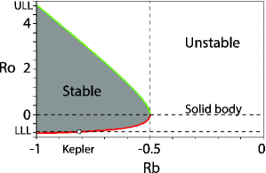
Figure 1: Dependence of the optimal critical Rossby numbers ${\rm Ro}_{\rm opt}^{\pm}$ on ${\rm Rb}$ when ${\rm Pm}=0$ and ${\rm N}\rightarrow 0$.

Having thus seen that HMRI can easily extend to Keplerian profiles, we still have to confirm that the shallow $B_{\phi}(r)$ profiles can indeed be produced by induction effects for which some finite value of ${\rm Rm}$ is still necessary. For the sake of illustration, we choose now ${\rm Ro}_{\rm Kep}=-3/4$, and ${\rm Ha}=30$. Figure 2 shows two groups of critical curves in the $\beta-{\rm Pm}$ plane. The four curves on the right side correspond to SMRI, the curves continuing into the left part correspond to HMRI. The latter ones consist, in general, of two parts, one reaching the inductionless ${\rm Pm}=0$ area. The connection between them typically happens at ${\rm Rm}\propto 1$.

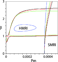
Figure 2: SMRI and HMRI for $n=0$, ${\rm Ro}=-3/4$, ${\rm Ha}=30$. Black: ${\rm Rb}=-0.74$, ${\rm Re}\approx 19876$, red: ${\rm Rb}=-0.75$, ${\rm Re}\approx 21294$, green: ${\rm Rb}=-0.77$, ${\rm Re}\approx 23935$, blue: ${\rm Rb}=-0.91$, ${\rm Re}\approx 38553$, middle of the blue curve ${\rm Pm}=0.0002$, $S={\rm Ha}{\rm Pm}^{1/2}\approx 0.42$, ${\rm Rm}={\rm Re}{\rm Pm}\approx 7.71$.

In Figure 3 we show that this mechanism is not restricted to $n=m=0$ but can easily extend to the range of AMRI with higher azimuthal wavenumbers $m$, both for small absolute values (Fig. 3a) and large absolute values (Fig. 3b) of $\beta$.

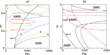
Figure 3: Domains of SMRI, HMRI, and AMRI for ${\rm Ha}=30$, ${\rm Ro}=-3/4$, ${\rm Re}=4000$, ${\rm Rb}=-0.755$, and (a) black: $n=-1$, blue: -2, green: -3, red: -4 and (b) red: $n=0$, black: 1.

In summary, we have found that the range of applicability of the inductionless versions of MRI that were previously thought to be restricted to ${\rm Ro}<{\rm Ro}_{\rm LLL}\approx-0.828$, can easily extend to Keplerian profiles if only ${\rm Rm}$ is large enough to produce a $B_{\phi}(r)$ profile that is somewhat shallower than $1/r$. Interestingly, the ${\rm Ro}_{\rm opt}^{+}({\rm Rb})$ curve starting with the ULL further continues to meet the ${\rm Ro}_{\rm opt}^{-}({\rm Rb})$ branch at the solid body rotation. Since this extension of the inductionless forms of MRI circumvents the usual demand $S\propto 1$, our finding may have significant consequences for the working of MRI in the colder parts of accretion disks. A detailed investigation of the respective roles of $S$ and $\rm Rm$ for the onset and the saturation mechanism of the instability in different astrophysical problems goes beyond the scope of this letter and must be be left for future work. We only note here that the sensitive structure of the instability domains in the low $\rm Pm$-region, as seen in Figs. 2 and 3, may easily trigger a quasi-oscillatory behaviour in the non-linear regime. Our results encourage experiments on the combination of MRI and current driven instabilities as they are presently planned in the framework of the DRESDYN project DRESDYN .

This work was supported by Helmholtz-Gemeinschaft Deutscher Forschungszentren (HGF) in frame of the Helmholtz Alliance LIMTECH, as well as by Deutsche Forschungsgemeinschaft in frame of the SPP 1488 (PlanetMag). We acknowledge fruitful discussions with Marcus Gellert, Rainer Hollerbach, and Günther Rüdiger.

References

- (1) S.A. Balbus, J.F. Hawley, Astrophys. J. 376, 214 (1991)
- (2) S.A. Balbus, P. Henri, Astrophys. J. 674, 408 (2008)
- (3) N.J. Turner, T. Sano, Astrophys. J. Lett. 679, L131 (2008)
- (4) W. Liu, J. Goodman, H. Ji, Astrophys. J. 643, 306 (2006)
- (5) A. Brandenburg et al., Astrophys. J. 446, 741 (1995); J. Herault et al., Phys. Rev. E 84, 036321 (2011)
- (6) S. Fromang, J. Papaloizou, Astron. Astrophys. 476, 1113 (2007)
- (7) J. Shi, J.H. Krolik, S. Hirose, Astrophys. J. 708, 1716 (2010)
- (8) P.J. Käpilä, M.J. Korpi, Mon. Not. R. Astr. Soc. 413, 901 (2011)
- (9) G. Lesur, P.-Y. Longaretti, Mon. Not. R. Astron. Soc. 378, 1471 (2007)
- (10) T.P. Fleming, J.M. Stone, J.F. Hawley, Astrophys. J. 530, 464 (2010); J.S. Oishi, M.-M. Mac Low, Astrophys. J. 740, 18 (2011); M. Flock, T. Henning, H. Klahr, Astrophys. J. 761, 95 (2012)
- (11) R. Hollerbach, G. Rüdiger, Phys. Rev. Lett. 95, 124501 (2005)
- (12) J. Priede, Phys. Rev. E 84, 066314 (2011)
- (13) W. Liu, J. Goodman, I. Herron, H. Ji, Phys. Rev. E 74, 056302 (2006)
- (14) F. Stefani et al., Phys. Rev. E. 80, 066303 (2009)
- (15) R. Hollerbach, V. Teeluck, G. Rüdiger, Phys. Rev. Lett. 104, 044502 (2010)
- (16) O.N. Kirillov, F. Stefani, Y. Fukumoto, Astrophys. J. 756, 83 (2012)
- (17) O.N. Kirillov, F. Stefani, Astrophys. J. 712, 52 (2010)
- (18) G. Rüdiger, R. Hollerbach, Phys. Rev. E 76, 068301 (2007)
- (19) O.N. Kirillov, F. Stefani, Phys. Rev. E 84, 036304 (2011)
- (20) O.M. Umurhan, Astron. Astrophys. 513, A47 (2010)
- (21) M. Seilmayer et al., Phys. Rev. Lett. 108, 244501 (2012)
- (22) E.R. Krueger, A. Gross, R.C. Di Prima, J. Fluid Mech. 24, 521 (1966); M.J. Landman, P.G. Saffman, Phys. Fluids 30, 2339 (1987); B. Eckhardt, D. Yao, Chaos, Solit., Fract. 5, 2073 (1995); S. Friedlander, M.M. Vishik, Chaos 5, 416 (1995)
- (23) H. Bilharz, Z. Angew. Math. Mech. 24, 77 (1944)
- (24) F. Stefani et al., Magnetohydrodynamics 48, 103 (2012)