The Atacama Cosmology Telescope: Beam Measurements and the Microwave Brightness Temperatures of Uranus and Saturn

Abstract

We describe the measurement of the beam profiles and window functions for the Atacama Cosmology Telescope (ACT), which operated from 2007 to 2010 with kilo-pixel bolometer arrays centered at 148, 218, and 277 GHz. Maps of Saturn are used to measure the beam shape in each array and for each season of observations. Radial profiles are transformed to Fourier space in a way that preserves the spatial correlations in the beam uncertainty, to derive window functions relevant for angular power spectrum analysis. Several corrections are applied to the resulting beam transforms, including an empirical correction measured from the final CMB survey maps to account for the effects of mild pointing variation and alignment errors. Observations of Uranus made regularly throughout each observing season are used to measure the effects of atmospheric opacity and to monitor deviations in telescope focus over the season. Using the WMAP-based calibration of the ACT maps to the CMB blackbody, we obtain precise measurements of the brightness temperatures of the Uranus and Saturn disks at effective frequencies of 149 and 219 GHz. For Uranus we obtain thermodynamic brightness temperatures $T_{\rm U}^{149}=$ $106.7\pm 2.2$ K and $T_{\rm U}^{219}=$ $100.1\pm 3.1$ K. For Saturn, we model the effects of the ring opacity and emission using a simple model and obtain resulting (unobscured) disk temperatures of $T_{\rm S}^{149}=$ $137.3\pm 3.2$ K and $T_{\rm S}^{219}=$ $137.3\pm 4.7$ K.

1. Introduction

The Atacama Cosmology Telescope (ACT) is a 6 m, off-axis telescope designed for millimeter wavelength observations of the cosmic microwave background (CMB) with arcminute resolution (Fowler et al., 2007). The telescope is located in Northern Chile, at an elevation of 5190 m, where atmospheric conditions are excellent for microwave observations from April through December. From 2008 to 2010, ACT observed the sky with bolometer arrays operating in frequency bands centered at 148 GHz, 218 GHz and 277 GHz. The choice of bands provides the ability, in principle, to spectrally discriminate between signal from the CMB, the Sunyaev-Zel’dovich effect (SZE; Sunyaev & Zel’dovich, 1970), and dusty sources. The 148 GHz array was also in operation during a short observing season at the end of 2007.

The ACT scientific program has produced measurements of the CMB angular power spectrum at multipoles spanning $\ell\approx 300$ to 10000 (Das et al., 2013; Dunkley et al., 2013), probing the primary and secondary anisotropies (Sievers et al., 2013). ACT has produced source catalogs (Marriage et al., 2011a), and galaxy cluster samples reaching to high redshifts (Marriage et al., 2011b; Hasselfield et al., 2013).

The telescope beam acts as a low-pass spatial filter on the astrophysical signal from the sky. The effects of this filtering are relevant, to varying degrees, to all ACT science results. Interpretation of the angular power spectrum, in particular, relies on its decomposition into components that are correlated across large ranges in angular scale. The extraction of cosmological parameters associated with such components depends on an understanding of the beam shape and the covariant features of the window function uncertainty.

In this work we describe the processing of planet observations to obtain the telescope beams, and thus the instrument window function, for each detector array for each season of operation. We also discuss the use of Uranus observations to monitor beam shape and calibration. Because the ACT maps are ultimately calibrated to the CMB blackbody via the dipole calibration of WMAP (Jarosik et al., 2011), we obtain precise measurements of the Uranus and Saturn disk temperatures without resorting to interpolation across unknown source spectra or other calibration transfer standards.

A detailed description of the instrument can be found in Swetz et al. (2011), and the main data reduction and map-making pipeline is described in Dünner et al. (2013). Hincks et al. (2010) present an analysis of the ACT beams from the 2008 season; the present approach extends this earlier analysis.

In Section 2 of this paper we discuss the planet observations and maps. In Section 3 we obtain the telescope window function through an analysis of the planet maps and the application of corrections for several systematic effects. In Section 4, we interpret the apparent brightness of Uranus to calibrate the sensitivity of the telescope to atmospheric water vapor and focus variation. In Section 5 we use the CMB-based calibration of the ACT maps to obtain absolutely calibrated measurements of Uranus and Saturn brightness temperatures.

2. Observations and Mapping

2.1. Observations

The ACT observation strategy is to scan over small ranges of azimuth angle while keeping the boresight altitude fixed at $\approx 50^{\circ}$ to minimize systematic effects due to altitude variation. The CMB fields are observed as they rise and set through two central azimuth pointings. Planet observations are made at this same telescope altitude angle, by briefly interrupting CMB survey scans and re-pointing in azimuth to the planet location.

ACT observed a planet approximately once per night of operation in 2007–2010, but only high quality observations of Saturn and Uranus are considered in this analysis. Saturn and Uranus were preferentially targeted, as Saturn’s brightness makes it useful for beam profile measurements, and Uranus’ stable brightness is a convenient calibration source. While Uranus was visible throughout each observing season, Saturn was available only at the beginning and end of each season. Jupiter and Mars were, respectively, too bright and too low in the sky to be useful for calibration work. In Table 1 we list the number of high quality Uranus and Saturn observations achieved in each season.

Table 1 Number of Saturn and Uranus observations selected for calibration purposes for each season and array.

	2007	2008	2009	2010
Saturn
148 GHz	022	022	013	035
218 GHz	–	023	009	028
277 GHz	–	016	005	023
Uranus
148 GHz	016	037	094	113
218 GHz	–	033	075	102
277 GHz	–	021	016	074

Note. — While Uranus was visible throughout each observing season, Saturn was available only near the beginning and end of each season. The number of successful planet observations is lower at higher frequencies because of increased sensitivity in these arrays to atmospheric contamination.

2.2. Planet Maps

As described in Dünner et al. (2013), maps are made from the ACT time stream data according to a maximum likelihood technique in which the noise is described in the time domain while the signal is assumed to be spatially coherent (Tegmark, 1997). The bolometer time stream data for planet observations are pre-processed in a similar fashion to the CMB survey data. The time stream data are calibrated, based on detector load curves, after deconvolving the effects of the detector time constants and low-pass readout filtering. Detectors are then screened for quality based on their projections onto a common-mode computed using a fiducial set of well-behaved detectors. Detector screening is performed with the planetary signal masked out. Maps are made using a dedicated code that is optimized for high resolution mapping of single observations; we have confirmed that the main season map pipeline code produces compatible results when run on the same data. Each map is solved iteratively, converging after fewer than 10 iterations. The noise model is designed to remove common-mode signal at frequencies below 0.2 Hz, corresponding to angular scales that are much larger than the array size. Because high-pass filtering of this kind may suppress signal at large angular scales, we study the transfer function of the map making solutions in Section 3.4.1.

2.3. Map Selection

While planets were observed almost every night, observations do not always yield successful maps. The primary reason for failed mapping is a low number of live detectors during periods of high sky loading. This is a greater problem at higher frequencies, and for the 277 GHz array in particular leads to many maps with incomplete sampling of the planet signal; such maps are discarded.

Planet observations are sometimes made after sunrise. While such observations allow us to study the magnitude of pointing and beam focus changes due to thermal deformation of the telescope structure, they are excluded from the present analysis. The sunrise cut is also applied to CMB observations.

A small number of maps are cut due to having substantially higher noise levels than other maps of the same planet for the same array and season. The remaining maps are used to establish the telescope beam and calibration parameters, as described in the following sections. Season mean beam maps, obtained by aligning and averaging the selected Saturn maps for each season and array, are shown in Figure 1. The Airy pattern is easily seen in the maps at 148 GHz and 218 GHz. The horizontal streaks are parallel to the telescope scan direction.

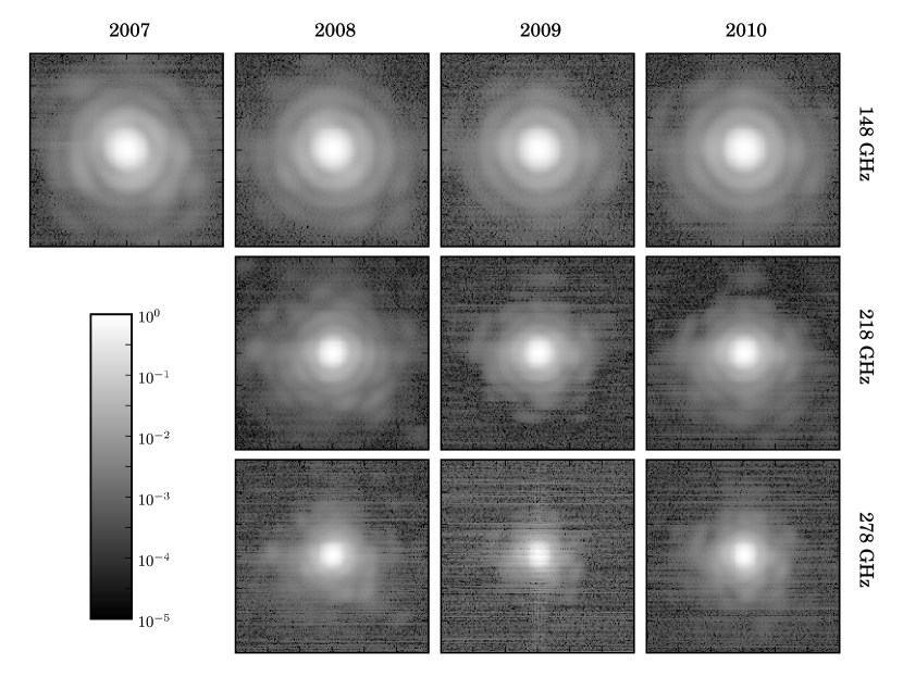
Figure 1.— Beam maps for each season and array, formed from the average of selected Saturn maps. Gray scale is logarithmic. Each panel is 12 ′ by 12 ′.Each contributing Saturn map incorporates all live detectors in the array. The well-resolved Airy rings indicates that the relative detector offsets are accurately known. The frequency labels correspond to the effective frequencies for CMB spectrum radiation (Swetz et al., 2011).

3. Beams

In this section we obtain measurements of the telescope beams for each season and array. Saturn is bright and much smaller than the beam solid angle, permitting the characterization of our beams with high signal-to-noise ratio. Saturn maps are reduced to radial profiles, which are then modeled with appropriately chosen basis functions and transformed to Fourier space. The resulting transform, the beam modulation transfer function, is corrected for a number of systematic effects to produce a window function and $\ell$-space covariance suitable for use with the ACT CMB survey maps.

3.1. Radial Profiles

While the instantaneous ACT beams are slightly ($<10\%$) elliptical in cross-section, we analyze them as though they were circular, and work exclusively with the “symmetrized” (i.e., azimuthally averaged) radial profiles. The resulting beam measurements are suitable for any analysis that incorporates a similar simple azimuthal average of the signal under study. In particular, the cross-linking of CMB survey observations is such that the telescope beam contributes to the map, with roughly equal weight, at two orientations that differ in rotation by approximately 90 degrees; the net effective beam is very nearly circular. The goal of our analysis is thus to characterize the symmetrized beam.

Radial profiles are obtained for each Saturn observation by averaging map data in radial annuli of width 9″, producing average profile measurements $y_{i}$ at radii $\theta_{i}$. On scales smaller than a few arcminutes, the covariant noise is sub-dominant to the planetary signal and thus the shape of the core beam is very well measured by even a single observation of Saturn. However, at larger angular scales there is non-negligible contamination from the atmosphere. This means that the asymptotic behavior of the beam cannot be separated from the fluctuating background without making some assumptions about the beam behavior far from the main lobe.

The illumination of the ACT optics is controlled by a cryogenic Lyot stop at an image of the circular exit pupil; this leads to a beam shape described by an Airy pattern (for monochromatic radiation) and to the expectation that the beam pattern (including the effects of finite detector size and spectral response) will decay asymptotically as $1/\theta^{3}$, where $\theta$ is the angle from the beam peak. We fit this model to the radial profile data in order to fix the background level of the map and to provide a model for extrapolating the beam to large angles.

The background level of the map and the large-angle behavior of the beam are measured by fitting the model $y(\theta)=A\times(1\mathrm{\SIUnitSymbolArcminute}{}/\theta)^{3}+c$ to the binned profile data in the range $\theta_{A}<\theta_{i}<\theta_{B}$, with the range chosen such that the profile measurements have fallen to below 1% of the peak but are still signal dominated. The points $y_{i}$ with $\theta_{i}<\theta_{A}$, corrected for the background level $c$ and renormalized so that $y(\theta=0)\approx 1$, constitute the “core” of the beam profile. The radial profile beyond $\theta_{A}$ is referred to as the “wing.” The fit ranges used for each array, and the amplitude of the beam at $\theta_{A}$ relative to the peak, are given in Table 2. An example of the wing fit for each array is shown in Figure 2.

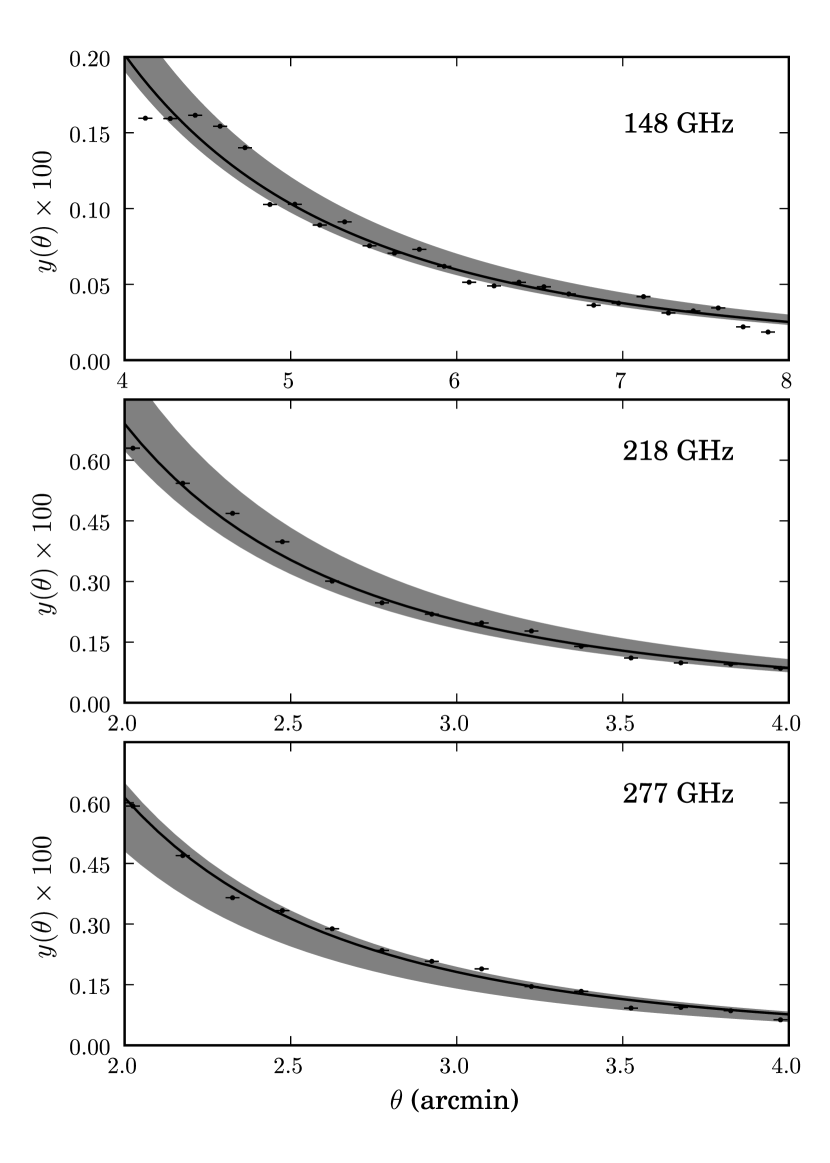
Figure 2.— Wing model fitted to binned radial profile data. Points shown, and the best-fit model (solid line) are from a typical individual Saturn observation for each array. A baseline is fit simultaneously and has been removed from the data points. The shaded area represents the standard deviation of all individual best-fits to wing models for the 2010 season.

Table 2 Summary of beam parameters by array and season.

		Wing Fit (§3.1)				Transform Fit (§3.2)			Beam Properties				Hincks et al
Array	Season	$\theta_{A}$	$\theta_{B}$	$B(\theta_{A})$		$\ell_{\rm max}$	$n_{\rm mode}$		Solid angle	FWHM	Ellip.		Solid angle
				$(10^{-3})$					($10^{-9}$ sr)	(arcmin)			($10^{-9}$ sr)
148 GHz	2007	4 ′	8 ′	2.40 $\pm$ 0.05		21900	11		$224.5\pm 1.4$	1.364 ′	1.098		–
	2008	4 ′	8 ′	2.03 $\pm$ 0.04		18400	9		$216.6\pm 1.6$	1.373 ′	1.065		$218.2\pm 4.0$
	2009	4 ′	8 ′	2.15 $\pm$ 0.09		16400	8		$215.8\pm 2.6$	1.378 ′	1.039		–
	2010	4 ′	8 ′	2.13 $\pm$ 0.04		15800	9		$215.4\pm 1.8$	1.381 ′	1.033		–
218 GHz	2008	2 ′	4 ′	6.54 $\pm$ 0.12		25500	6		$116.5\pm 1.1$	1.092 ′	1.021		$118.2\pm 3.0$
	2009	2 ′	4 ′	7.07 $\pm$ 0.29		25800	6		$123.9\pm 1.7$	1.057 ′	1.026		–
	2010	2 ′	4 ′	7.34 $\pm$ 0.21		25100	6		$125.0\pm 1.8$	1.015 ′	1.027		–
277 GHz	2008	2 ′	4 ′	5.49 $\pm$ 0.12		28400	7		$\phantom{0}98.1\pm 1.9$	0.869 ′	1.049		$104.2\pm 6.0$
	2009	2 ′	4 ′	5.22 $\pm$ 0.26		32100	7		$\phantom{0}95.2\pm 4.0$	0.879 ′	1.118		–
	2010	2 ′	4 ′	5.65 $\pm$ 0.18		28600	7		$\phantom{0}98.9\pm 2.0$	0.870 ′	1.103		–

Note. — Radial profiles are obtained within a distance $\theta_{A}$ from the peak; wing and baseline parameters are fit to data over the range $\theta_{A}$ to $\theta_{B}$. The level $B(\theta_{A})$ of the beam, relative to the peak, at the edge of the wing fit region is shown for reference. Parameters $\ell_{\rm max}{}$ and $n_{\rm mode}$ describe the basis functions used for fitting a beam model to the radial profile data in the beam core. The solid angle and FWHM of the symmetrized instantaneous telescope beam are provided, along with the ellipticity (defined as the ratio of major to minor axes of the unsymmetrized mean beam). The solid angles for the 2008 season may be compared to the values from the independent analysis of Hincks et al. (2010).

For each array, the multiple observations of Saturn in each season are combined by taking the mean of their core profile points and wings. The season mean beam profile is thus described by points $\mathrm{bar}{y}_{i}$ (for each $\theta_{i}<\theta_{A}$) and a mean wing fit parameter $\mathrm{bar}{A}$. The full covariance matrix of $\{\mathrm{bar}{y}_{1},...,\mathrm{bar}{y}_{n},\mathrm{bar}{A}\}$ is computed from the ensemble of Saturn profiles and, as described in the next section, is used to propagate covariant error on large angular scales into the $\ell$-space beam covariance matrix.

The solid angle and FWHM of the beam (as well as the approximate ellipticity of the non-symmetrized telescope beam) are shown in Table 2. Solid angles may be compared to the values presented in Hincks et al. (2010). The reduction in solid angle uncertainty is primarily due to our choice to fit the wing over a range of radii closer to the beam center. We have doubled the error from its formal value to account for systematic variation in solid angle results as different fitting ranges are used.

3.2. Harmonic Transforms and Window Functions

Sky temperature data may be compared to predictions based on cosmological models through statistical measures such as the angular power spectrum of temperature fluctuations. The effect of the observing strategy and telescope beam on the measurement of correlation functions in CMB data has been discussed in, e.g., White & Srednicki (1995). For ACT, it is important to understand the beam and its covariance over a broad range of angular scales.

A Gaussian random temperature field $T({\mathbf{n}})$ at position ${\mathbf{n}}$ on the sphere may be characterized by coefficients $C_{\ell}$ of the decomposition of its auto-correlation function:

$$\Big{\langle}T({\mathbf{n}})T({\mathbf{n^{\prime}}})\Big{\rangle} =\sum_{\ell=1}^{\infty}\frac{2\ell+1}{4\pi}C_{\ell}P_{\ell}({\mathbf{n}}\cdot{\mathbf{n^{\prime}}}),$$ (1)

where $P_{\ell}$ are Legendre polynomials. Measurements $\widetilde{T}({\mathbf{n}})$ of the temperature field with a given telescope and observing strategy will differ from the true sky temperature; for ACT the primary effects are an uncertain calibration (which we neglect for now) and the telescope beam. For the case of an azimuthally symmetric beam that does not vary in time or with position on the sky, the auto-correlation function of the observed temperature map $\widetilde{T}{}({\mathbf{n}})$ will be related to the $C_{\ell}$ describing the $T({\mathbf{n}})$ by (e.g., White & Srednicki, 1995)

$$\left\langle\widetilde{T}{}({\mathbf{n}})\widetilde{T}{}({\mathbf{n^{\prime}}})\right\rangle =\sum_{\ell}\frac{2\ell+1}{4\pi}C_{\ell}P_{\ell}({\mathbf{n}}\cdot{\mathbf{n^{\prime}}})B_{\ell}^{2},$$ (2)

where $B_{\ell}$ are the multipole coefficients of the beam, defined by

$$B(\theta) =\sum_{\ell=1}^{\infty}B_{\ell}\sqrt{\frac{(2\ell+1)}{4\pi}}P_{\ell}(\cos\theta).$$ (3)

In this context, $B_{\ell}^{2}$ is referred to as the window function.

The ACT beams are sufficiently concentrated that we may work in a flat sky approximation and take $\theta$ to be a radial coordinate in the plane. The radial component of the Fourier conjugate variable will be $\ell$. The azimuthally symmetric two-dimensional Fourier transform $B(\ell)$ of $B(\theta)$ may be used to obtain the multipole coefficients according to $B_{\ell}=B(\ell)$ with entirely negligible error. We will thus work in the flat sky approximation, but write $B_{\ell}$ (with $\ell$ in subscript) to emphasize the correspondence to the multipole coefficients.

We consider contributions from the wing and from the core separately. The transform of the wing (which is truncated below $\theta_{A}$) is easily obtained. For the beam core, computation of the transform from the binned radial profile requires us to interpolate the profile data $y_{i}$. We achieve this by expressing the real space beam as a sum of basis functions which we know to have spatial frequency cut-offs near those determined by the telescope optics in each frequency band.

The primary mirror has a diameter $D=6$ m; this size limits the optical response to spatial frequencies below $\ell_{\rm max}{}\approx 2\pi D/\lambda$. A natural basis for the Fourier space beam is then provided by the Zernike polynomials $R_{2n}^{0}(\rho)$, where $\rho=\ell/\ell_{\rm max}{}$. (The Zernike polynomials $R_{n}^{m}(\rho,\phi)$ are orthogonal and complete on the unit disk; here we impose azimuthal symmetry and need only consider even $n$ and $m=0$.) We thus model the real space beam with basis functions $f^{n}(\theta)$, for non-negative integer $n$, that are proportional to inverse Fourier transforms of $R_{2n}^{0}(\rho)$:

$$f^{n}(\theta) =\frac{J_{2n+1}(\theta\ell_{\rm max}{})}{\theta\ell_{\rm max}{}}.$$ (4)

In practice, for some value of $\ell_{\rm max}{}$ and a mode count $n_{\rm mode}$ the beam model is expressed as

$$B(\theta) =\sum_{n=0}^{n_{\rm mode}-1}a^{n}f^{n}(\theta),$$ (5)

where the coefficients $a^{n}$ are fit parameters. The model is fitted to the data by minimizing the $\chi^{2}$ of the residuals $y_{i}-B(\theta_{i})$, accounting for the full covariance of the $y_{i}$ measurements. Values of $\ell_{\rm max}{}$ and $n_{\rm mode}$ are adjusted to obtain a fit with the minimum number of modes necessary that gives a $\chi^{2}$ per degree of freedom equal to unity. The fit yields coefficients $a^{n}$ and the covariance matrix of the errors, $\langle\delta a^{n}\delta a^{n^{\prime}}\rangle$.

Details of the fitting parameters, including $\ell_{\rm max}{}$, $n_{\rm mode}$ and reduced $\chi^{2}$ for each season and array, are presented in Table 2. The choice of basis functions results in a satisfactory expansion of the beam using approximately half as many modes as data points.

After fitting the coefficients $a^{n}$ in real space, we obtain the corresponding beam transform,

$$B_{\ell} =\sum_{n}a^{n}F^{n}_{\ell}+w_{\ell},$$ (6)

where $F^{n}_{\ell}$ are the Fourier transforms of $f^{n}(\theta)$, truncated above $\theta_{A}$, and $w_{\ell}$ is the Fourier transform of the extrapolated wing, from $\theta_{A}$ to infinity.

The resulting beam transforms are shown in Figure 3. While the beams for the 2008 season are shown, the beam features are not substantially different between seasons. The figure shows the separate contributions of the core and wing to the beam transform. The wing contributes significantly only at low $\ell$ (i.e., below 1000 at 148 GHz, and below 2000 at 218 GHz and 277 GHz).

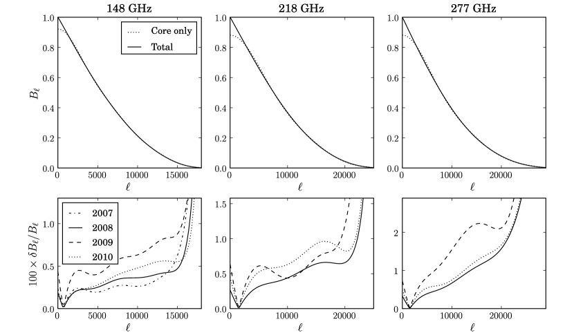
Figure 3.— Upper panels: Beam transforms $B_{\ell}$ for each array. Beams shown are for the 2008 season. The total beam is the sum of the contribution from the core of the beam, and the extrapolated wing. Lower panels: Diagonal error from the covariance matrix for the renormalized beam. The beam normalization has been fixed at calibration $\ell$ = 700 (1500) for the 148 GHz (218 GHz and 277 GHz) array(s), as described in Section 3.3. Note that these curves show uncertainty, not systematic trends, and they do not include additional uncertainty from the empirical corrections of Section 3.5. The full covariance matrix shows an anti-correlation between the beam error at angular scales above the calibration $\ell$ and beam error below the calibration $\ell$. The window function is $B_{\ell}^{2}$ and thus its fractional error is $2\delta B_{\ell}/B_{\ell}$.

While this is very similar to the procedure described in Hincks et al. (2010), in this work we include covariance between radial profile data points, and between the radial profile and the wing fit parameter. This results in a natural propagation of beam errors on all spatial scales into the fitted beam transform and its $\ell$-space covariance matrix. Our treatment of beam errors is discussed in the next section.

3.3. Beam and Calibration Covariance

Using the covariance matrix of the fit coefficients obtained in Section 3.1, we also obtain the covariance in $\ell$ space:

$$\Sigma_{\ell\ell^{\prime}} \equiv\left\langle\delta B_{\ell}\delta B_{\ell^{\prime}}\right\rangle$$

$$=\sum_{n,n^{\prime}}F^{n}_{\ell}F^{n^{\prime}}_{\ell^{\prime}}\left\langle\delta a^{n}\delta a^{n^{\prime}}\right\rangle+\left\langle\delta w_{\ell}\delta w_{\ell^{\prime}}\right\rangle$$

$$\quad+\sum_{n}F_{\ell}^{n}\left\langle\delta a^{n}\delta w_{\ell^{\prime}}\right\rangle+\sum_{n}\left\langle\delta w_{\ell}\delta a^{n}\right\rangle F_{\ell^{\prime}}^{n}.$$ (7)

This covariance includes contributions from the wing fit error and the correlation between the wing fit error and the coefficients $a^{n}$.

This covariance matrix is an $\ell$-space representation of the covariant features in the radial profiles that contribute to the $B_{\ell}$. However, because the calibration of the CMB survey maps is established at a particular angular scale, we must recast the beam covariance into an appropriate form. This is effectively the same procedure applied in Page et al. (2003).

The absolute calibration of the ACT maps at 148 GHz is obtained by cross-correlation of the 2008 Southern and 2010 Equatorial maps with the WMAP 7-year maps (Jarosik et al., 2011) at 94 GHz of the same sky region, over angular scales with $300<\ell<1100$ (Hajian et al., 2011; Das et al., 2013). This leads to an absolute calibration of the ACT maps centered near $\ell=700$. The 2009 season Equatorial maps at 148 GHz are then calibrated, over $500<\ell<2500$, to the 2010 season Equatorial maps. The subsequent calibration of the 218 GHz maps to the 148 GHz maps is performed in the signal-dominated regime with $1000<\ell<3000$. The 277 GHz maps have not yet been calibrated to WMAP. For each season and array, we factor out the beam amplitude at effective calibration scale $\ell=L$, where $L=700$ for the 148 GHz array, and $L=1500$ for the 218 GHz and 277 GHz arrays.

For a celestial temperature signal described by multipole moments $T_{\ell,m}$, we measure a map $M_{\ell,m}$ in detector power units, which is related to $T$ by

$$M_{\ell,m} =G_{\ell}T_{\ell,m},$$ (8)

where $G_{\ell}\equiv G_{0}B_{\ell}$ is the product of the beam (normalized such that $B_{\ell=0}=1$) and a global calibration factor $G_{0}$ that converts CMB temperature to map units (i.e., to detector power units).

Our calibration to WMAP is a comparison of $M$ and $T$ at $\ell=L$ and is thus a measurement of $G_{L}$ that is independent of our beam uncertainty. This leads us to recast Equation (8) as

$$M_{\ell,m} =G_{L}b_{\ell}T_{\ell,m},$$ (9)

where

$$b_{\ell}\equiv\frac{B_{\ell}}{B_{L}}.$$ (10)

Since the errors in $b_{\ell}$ and $G_{L}$ are not correlated, the uncertainty in $G_{\ell}$ is described by a covariance matrix $\Gamma_{\ell\ell^{\prime}}$ that is the sum of a calibration error from the measurement of $G_{L}$, and a term due to correlated error in the $b_{\ell}$:

$$\Gamma_{\ell\ell^{\prime}} =b_{\ell}b_{\ell^{\prime}}(\delta G_{L})^{2}+\frac{G_{L}^{2}}{B_{L}^{2}}\left[\Sigma_{\ell\ell^{\prime}}-b_{\ell}\Sigma_{L\ell^{\prime}}\right.$$

$$\left.\phantom{0000000000000000}-\Sigma_{\ell L}b_{\ell^{\prime}}+b_{\ell}b_{\ell^{\prime}}\Sigma_{LL}\right].$$ (11)

The term in square brackets is the normalized beam covariance that accompanies ACT data releases. The diagonal beam error (i.e., the square root of the diagonal entries of the normalized beam covariance) is shown for each season and array in Figure 3. At high $\ell$, the error in the effective season beam is dominated by an empirical map-based correction, which is not included here (see Section 3.5).

While the fitted beam and covariance are an accurate description of the binned radial beam profile, they must be corrected for a number of systematic effects prior to being used to interpret ACT maps.

3.4. Correction for Systematics

The beams computed in the preceding section are corrected for a number of systematic effects that would otherwise bias the resulting transforms relative to the true telescope beam. These are briefly described below.

3.4.1 Mapping Transfer Function

Because our map-making procedure includes time domain high-pass filtering, we might expect poor reproduction of large spatial scales. We study the mapping transfer function by injecting a simulated signal into telescope time stream data and comparing the output map to the input map in Fourier space. The transfer function deviates significantly from unity only on angular scales larger than 20 ′. The wing fit is performed at somewhat smaller radii than this, and we have confirmed that the wing fit and extrapolation reproduces the input signal, on all scales, to 0.1%.

A very small ($\approx$0.1%) correction due to the 3.5″ pixelization of the planet maps is applied by dividing the beam transform by the azimuthal average of the analytic pixel window function.

3.4.2 Radial Binning of Planet Maps

The binning of the planet map pixel data into annuli has a slight impact on the inferred beam transform. This is quantified by evaluating the harmonic transform of data points taken from a model of the radial beam profile, and comparing it to the harmonic transform of points that include simulated binning of the radial beam profile. This resulting correction is approximately 1% at $\ell=10000$.

3.4.3 Saturn Disk and Ring Shape

The Saturn angular diameter of approximately 8″ is large enough that we do not treat it as a point source. For each season and array, we deconvolve Saturn’s shape assuming that it is a disk with solid angle equal to the mean solid angle for all Saturn observations that contribute to the mean instantaneous beam measurement. This correction is approximately 2% at $\ell=10000$.

While Saturn’s rings complicate the spatial distribution of the planetary signal, these effects are negligible at $\ell<20000$, aside from an overall change in average brightness, and need not be considered in the deconvolution procedure.

3.5. Mean Instantaneous vs. Effective Beam

After applying the corrections described in Section 3.4, the resulting beam describes the telescope response to a point-like radiation source with approximately Rayleigh-Jeans spectrum, averaged over the focal plane of each array. We refer to this beam as the “mean instantaneous beam,” to emphasize that the combination of observations taken at many different times may lead to an effective window function that is different from the instantaneous one.

For use in particular contexts, we compute an effective beam that includes corrections for alternative frequency spectra, and for pointing variation or other cumulative effects resulting from the combination of observations taken at many different times.

We apply a simple first-order correction to obtain the effective beam for different radiation spectra. For radiation with a band effective frequency $\nu$, the beam is taken to be

$$B^{\prime}(\ell) =B(\ell\nu_{\rm RJ}/\nu),$$ (12)

where $\nu_{RJ}$ is the effective frequency for radiation with a Rayleigh-Jeans (RJ) spectrum. Effective frequencies for various spectral types are presented in Swetz et al. (2011).

In the absence of planetary sources, the absolute pointing registration of individual ACT observations is not known. Since each pixel of the ACT survey maps contains contributions from data acquired on many different nights throughout each season, the resulting season effective beam for these maps is less sharp than the instantaneous beam obtained from carefully aligned individual planet observations.

Pointing repeatability can be estimated from the variation in apparent planet positions, relative to expectations, in each season and array. As summarized in Table 3, these indicate that the repeatability of telescope pointing is at the $\sigma_{\rm planet}=3\arcsec{}$ to 8″ (RMS) level. Pointing variation in CMB observations may in principle be smaller than $\sigma_{\rm planet}$, since CMB observations are performed at the same azimuth angles each night, while planets observations span a wider range of azimuths.

In addition to pointing repeatability, the season effective beam may also be diluted due to errors in the global pointing model, which is used to combine observations made at different azimuth angles. These global adjustments are estimated using point source positions measured in (non-cross-linked) maps made from only rising or only setting data.

While pointing variance and global alignment may contribute to dilution of the season beam, we must also acknowledge that the beam may change slightly over the course of the season in a way that is not captured by the Saturn observations. (Changes in the beam over the course of the season, and the resulting impact on calibration, are assessed using Uranus observations in Section 4.) We thus seek an empirical measure of the difference between the season effective beam and the instantaneous beam obtained from Saturn observations.

We parametrize the difference between the season effective beam $B_{\ell}^{\rm eff}$ and the instantaneous beam $B_{\ell}$ as a Gaussian in $\ell$:

$$B_{\ell}^{\rm eff} =B_{\ell}\times e^{-\ell(\ell+1)V/2}.$$ (13)

If the correction is interpreted as arising purely from Gaussian pointing error, then $V$ is simply the pointing variance in square radians. While this motivates the form of the correction, our broader interpretation permits $V$ to differ from the value expected based on pointing variance measured from planets, or to be less than zero if the season effective beam is somewhat sharper than the ensemble of Saturn observations indicates.

We measure $V$ for each season and array using bright point sources in the season CMB survey maps. Point sources with signal to noise ratios greater than 10 are identified using a matched filter. A beam model is fit to the map in the vicinity of each source, producing a value of $V$. The weighted mean and error of these individual fits, for each season and array, are used to form the effective beam for use with the survey maps. While this point source analysis gives us a secondary probe of the beam core, we note that the Saturn observations are still key for measuring the behavior in the wings of the beam.

The values of the season correction parameter $V$ are presented in Table 3. The measurement of $V$ is somewhat susceptible to changes in the fitting parameters and thus the quoted errors have been inflated from the formal values by factors of 2 and 6 for the 148 GHz and 218 GHz arrays, respectively. While values of $V$ for the 148 GHz array are very similar between seasons, values for 218 GHz are more variable. The analysis of Uranus observations in Section 4.1 shows that in 2010 the telescope beam was more sharply focused, relative to the mean beam estimated from Saturn, during most of the observing season (see Section 4.1); this results in a negative value for $V$ at 218 GHz.

Table 3 Pointing variance and beam correction parameters.

		$\sigma^{2}_{\rm planet}$	$V$	Attenuation
Season	Array	(arcsec2)	(arcsec2)	at $\ell=5000$
2007	148 GHz	-$\phantom{0}53\pm 12$	–	–
2008	148 GHz	-$\phantom{0}24\pm\phantom{0}4$	-$\phantom{0}25\pm 10$	-$0.993\pm 0.003$
	218 GHz	-$\phantom{0}23\pm\phantom{0}5$	-$143\pm 51$	-$0.962\pm 0.013$
	277 GHz	-$\phantom{0}11\pm\phantom{0}2$	–	–
2009	148 GHz	-$\phantom{0}58\pm\phantom{0}9$	-$\phantom{0}26\pm\phantom{0}6$	-$0.993\pm 0.002$
	218 GHz	-$\phantom{0}43\pm\phantom{0}8$	-$\phantom{0}46\pm 27$	-$0.988\pm 0.007$
	277 GHz	-$\phantom{0}49\pm 18$	–	–
2010	148 GHz	-$\phantom{0}31\pm\phantom{0}3$	-$\phantom{0}29\pm\phantom{0}6$	-$0.992\pm 0.002$
	218 GHz	-$\phantom{0}18\pm\phantom{0}2$	-$5\pm 23$	-$1.002\pm 0.006$
	277 GHz	-$\phantom{0}25\pm\phantom{0}3$	–	–

Note. — Pointing variance $\sigma_{\rm planet}^{2}$ is measured from planet observations, and the season effective beam correction parameter $V$ is measured from point sources in the full-season CMB survey maps, where available. The parameter $V$ is used to correct the high-$\ell$ beam for use with the survey maps; the resulting attenuation or inflation of the beam at $\ell=5000$ is provided for reference. The covariant error due to this correction is included in the season effective beam covariance matrix.

4. Planet Brightness Measurements

In this section we use observations of Uranus and Saturn to study the variation in the system gain due to changes in water vapor level and telescope focus.

4.1. Planet Amplitudes

We characterize the apparent brightness of a planet in a map by examining the ratio of the Fourier transform of the map to expectations based on the beam and planet shape. While ultimately equivalent to procedures that involve measuring source peak heights in filtered real-space maps, the Fourier space approach emphasizes the role of spatial filtering in providing precise planet amplitude measurements. It also allows us to quantify differences between the planet shape and expectations based on the beam measurements in a physically meaningful way.

Once again working in the flat sky limit, we let $\theta$ represent a vector in the plane of the sky centered on the planet. The Fourier conjugate variable is denoted as $\ell$ and is written in subscript. The signal from a planet is modeled as a circular disk of uniform RJ temperature $T^{P}$. For each planet observation, we use the total disk solid angle $\Omega^{P}$ to compute angular radius $\theta^{P}\equiv(\Omega^{P}/\pi)^{1/2}$. The Fourier transform of the planetary signal has components

$$T_{\ell} =T^{P}\Omega^{P}_{\ell},$$ (14)

where $\Omega^{P}_{\ell}\equiv\Omega^{P}\times(2J_{1}(\ell\theta^{P})/(\ell\theta^{P}))$ is the Fourier transform of a disk of radius $\theta^{P}$. For Uranus, $\Omega^{P}_{\ell}\approx\Omega^{P}$ at the ACT angular scales; for Saturn, the finite disk size cannot be neglected, but the effects due to its oblateness are negligible. Planetary radii are taken at the 1 bar atmospheric surface, as reported in Archinal et al. (2011). The Saturn equatorial radius is $60268\pm 4$ km and the polar radius is $54364\pm 10$ km; the Uranus equatorial radius is $25559\pm 4$ km and the polar radius is $24973\pm 20$ km.

Adapting equation (8) to the flat sky, the ACT map $M(\mbox{\boldmath$\theta$}{})$ of the planetary signal will have Fourier components

$$M_{\mbox{\boldmath$\ell$}}{} =G_{0}B_{\ell}T^{P}\Omega^{P}_{\ell}.$$ (15)

For each planet map, we compute the amplitude $M_{\ell}$ of the planet at multiple bins in $\ell$. The map is centered, apodized, and Fourier transformed. To suppress atmospheric contamination, which contributes faint horizontal streaks to the map, we mask Fourier components having $|\ell_{x}|<1700$. The remaining complex Fourier amplitudes are averaged inside annuli of width $\Delta\ell\approx 600$ and the imaginary part is discarded. We then compute the ratio of $M_{\ell}$ to $B_{\ell}\Omega^{P}_{\ell}$ (which has been corrected to account for the apodization and masking applied to obtain $M_{\ell}$).

The result is a curve of planet amplitude measurements,

$$\widehat{\alpha}{}_{\ell} \equiv\frac{M_{\ell}}{B_{\ell}\Omega^{P}_{\ell}},$$ (16)

for $2000<\ell<14000$. In the absence of any gain or beam variation, $\alpha_{\ell}$ should be equal to $G_{0}T^{P}$, the apparent brightness of the planet in detector power units.

The mean and variance of $\widehat{\alpha}{}_{\ell}$ curves for selected seasons and arrays are shown in Figure 4. The $\widehat{\alpha}{}_{\ell}$ curves are not in all cases consistent with a constant value. This may be attributed to variations in the focus from night to night. To parametrize these deviations and to make possible an assessment of the impact they might have on the system calibration, we fit parameters $\widehat{\alpha}{}$ and $\widehat{\beta}{}$ for each $\widehat{\alpha}{}_{\ell}$ curve according to the following model:

$$\widehat{\alpha}{}_{\ell} =\widehat{\alpha}{}\left(1+\widehat{\beta}{}\frac{\ell-\mathrm{bar}{\ell}}{5000}\right).$$ (17)

The mean angular scale $\mathrm{bar}{\ell}$ is taken as the center of the fitting range. The parameters $\widehat{\alpha}{}$ and $\widehat{\beta}{}$ represent the mean amplitude of the planet and the deviation from expected focus of the beam, respectively. For example, $\widehat{\beta}{}=0.01$ would indicate that the the planetary signal is stronger by 1% at $\ell\approx 10000$ relative to $\ell\approx 5000$, given the mean season beam, and thus the telescope beam at the time of observation was slightly more sharply focused. We would expect observations associated with negative $\widehat{\beta}{}$ to also have a smaller $\widehat{\alpha}{}$ than expected, since a less sharply focused beam will have poorer overall efficiency.

The extraction of amplitudes $\widehat{\alpha}{}$ and focus parameters $\widehat{\beta}{}$ allows us to quantify deviations of focus over the season, and to estimate the effects of such deviations on the overall system calibration. This is accomplished in the next section, where a model for system calibration is obtained from the brightness and focus measurements of Uranus.

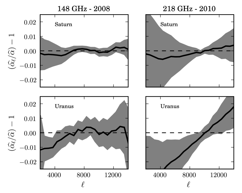
Figure 4.— Variation of planet amplitude measurements with angular scale. Each panel shows mean fractional deviation of $\widehat{\alpha}{}_{\ell}$ relative to $\widehat{\alpha}{}$ (solid line) and the standard deviation of all individual $\widehat{\alpha}{}_{\ell}/\widehat{\alpha}{}$ curves (grey band) for a particular season, array, and planet. See Section 4.1 for definitions of $\widehat{\alpha}{}_{\ell}$ and $\widehat{\alpha}{}$. We show results from 148 GHz 2008 (left panels), where there is a high degree of consistency between the planet observations and the season mean beam. We also show results for 218 GHz 2010 (right panels), where there is somewhat more variance in the curves (which is typical of the 218 GHz array) and where the Uranus observations deviate significantly from the mean beam (which is seen in all arrays in 2010). Differences between Uranus and Saturn are indicative of 2% changes in the beam focus during the season; such changes have been accounted for in the season effective beam by fitting a correction parameter to maps of point sources in the season maps as described in Section 3.5.

4.2. Calibration Parameters from Uranus Observations

The measurements of $\widehat{\alpha}{}$ and $\widehat{\beta}{}$ from Uranus observations, along with measurements of the precipitable water vapor (PWV) level for most of these observations, permit us to characterize the impact of PWV level and focus variation on the telescope calibration. This analysis does not require that the brightness temperature of Uranus be precisely known, but assumes that the brightness is roughly constant over the observing season. (We do not perform the same analysis on Saturn, because the effective brightness varies with the ring opening angle; see Section 5.2).

The Atmospheric Transmission at Microwaves model (ATM; Pardo et al., 2001) provides estimates of atmospheric emission and absorption at millimeter and sub-millimeter wavelengths. The ACT frequency bands avoid strong molecular resonances and are thus primarily susceptible to continuum emission and absorption due to water vapor. For the purposes of calibration we are interested in the atmospheric transmission in a given frequency band. The transmission at the ACT observation altitude $\theta_{0}$ is written as

$$T =\exp\left(-(\tau_{\rm w}{}w+\tau_{\rm d}{})/\sin\theta_{0}\right),$$ (18)

where $w$ is the precipitable water vapor column density at zenith and $\tau_{\rm w}{}w$ and $\tau_{\rm d}{}$ are the “wet” and “dry” optical depths at zenith. The parameters $\tau_{\rm w}{}$ and $\tau_{\rm d}{}$ vary negligibly over the range of temperatures and pressures experienced at the telescope site.

Because planet observations discussed in this work are obtained at the same fiducial altitude used for CMB observations, the effects of $\tau_{\rm d}{}$ are common to both observations and cannot be measured from the planet observations. We define the overall system gain $G_{0}$ such that it applies at the typical PWV level of $w_{0}=0.44$ mm. The $w$-dependent gain factor is then

$$G_{0}(w) =G_{0}\exp\left(-(\tau_{\rm w}{}+\tau_{\rm x}{})(w-w_{0})/\sin\theta\right).$$ (19)

Here $\tau_{\rm w}{}$ is as provided by the ATM model, while $\tau_{\rm x}{}$ is a fit parameter that could indicate a deviation from the ATM model but is more likely due to a bias in the detector calibration procedure that is sensitive to sky loading. Estimates of $\tau_{\rm w}{}$ for the ACT bands were computed using the ATM model by Marriage (2006); these values are provided for reference in Table 4.

To assess the impact of small variations in telescope focus on planet calibration, we include a dependence on the difference between the focus parameter $\widehat{\beta}{}$ (defined in Equation (17)) and the season mean focus parameter $\mathrm{bar}{\beta}$. Because a planet was observed approximately once per night, we take $\mathrm{bar}{\beta}$ to be the average of measured $\widehat{\beta}{}$ for all planet observations for the array and season under consideration. We adopt an exponential form out of convenience; calibration variation is small so a linear correction would be equivalent.

The full model for the Uranus brightness data $\widehat{\alpha}{}$, $\widehat{\beta}{}$ is then given by

$$\alpha =T^{U}G_{0}e^{m(\beta-\mathrm{bar}{\beta})}\times$$

$$\quad\quad\exp\left(-(\tau_{\rm w}{}+\tau_{\rm x}{})(w-w_{0})/\sin\theta\right),$$ (20)

where the fit parameters $T^{U}G_{0}$, $m$, and $\tau_{\rm x}{}$ represent overall calibration, sensitivity to variations in telescope focus, and sensitivity to PWV beyond predictions based on ATM, respectively.

This model is fitted to the Uranus brightness amplitude data for each season and frequency array. The parameter values are presented in Table 4. The residuals have scatter of approximately 2%, 2% to 6%, and 6% in the 148 GHz, 218 GHz and 277 GHz arrays respectively; this scatter is not explained by uncertainties in planet amplitude measurement. Values obtained for $\tau_{\rm x}{}$ are in good agreement between seasons for the 148 GHz and 218 GHz arrays. They are inconsistent with zero (at the $\approx 2$–$\sigma$ to 4–$\sigma$ level), which we attribute to systematic detector calibration error. For the 277 GHz array there is some slight disagreement between the 2009 and 2010 results, which we attribute to the low number of observations in 2009. The values of $\tau_{\rm x}{}$ are used in combination with $\tau_{\rm w}{}$ to correct the time-ordered data for opacity prior to creation of full-season survey maps, as described in Dünner et al. (2013).

While for some seasons and arrays we obtain better fits to the data by including the parameter $m$, the impact of this additional parameter on inferred overall system calibration is small. To show this, we refit the model of equation (20) with parameter $m$ fixed to 0. The resulting calibration factor $T^{U}G_{0}^{(m=0)}$ may be compared to the case where $m$ was free to vary. The differences are presented in Table 4; the change in overall calibration is 0.6% or smaller, and always less than the 1-$\sigma$ error on $T^{U}G_{0}$, with the exception of the 2009 data for the 218 GHz array. This exceptional case also has a large (9%) uncertainty in its absolute WMAP-based calibration.

The fit values of $T^{U}G_{0}$ may be used to provide an absolute calibration of each array (should $T^{U}$ be known) or to provide a measurement of the Uranus disk temperature based on an independent calibration of $G_{0}$. The latter possibility is discussed in the next section, leading to the measurements of Uranus and Saturn brightness temperatures presented in Section 5.

Table 4 Properties of planetary data and calibration model fit parameters by season and array.

	Array
Quantity	148 GHz	218 GHz	277 GHz
$\tau_{\rm w}$ (mm-1)	$0.019$	$0.044$	$0.075$
$\tau_{\rm x}$ (mm-1)
2007	-$0.016\pm 0.010$	–	–
2008	-$0.014\pm 0.004$	-$0.040\pm 0.008$	-$0.033\pm 0.063$
2009	-$0.009\pm 0.005$	-$0.021\pm 0.017$	-$0.008\pm 0.041$
2010	-$0.012\pm 0.003$	-$0.045\pm 0.008$	-$0.083\pm 0.016$
Error in $T^{U}G_{0}$ (%)
2007	0.9	–	–
2008	0.2	0.4	1.3
2009	0.3	1.1	2.2
2010	0.2	0.4	0.8
$m$
2007	-$0.7\pm 0.6$	–	–
2008	-$0.5\pm 0.3$	-$0.5\pm 0.6$	-$1.2\pm 1.3$
2009	-$0.5\pm 0.3$	-$3.4\pm 0.5$	-$1.2\pm 0.7$
2010	-$0.8\pm 0.1$	-$0.5\pm 0.2$	-$1.5\pm 0.4$
$\beta$ mean (rms)
2007	$-$0.017 (0.010)	–	–
2008	0.002 (0.006)	0.011 (0.010)	0.011 (0.015)
2009	0.004 (0.011)	0.008 (0.016)	0.007 (0.020)
2010	0.015 (0.015)	0.021 (0.019)	0.017 (0.019)
$\left(G_{0}^{(m=0)}/G_{0}-1\right)$ (%)
2007	$-$0.6	–	–
2008	0.1	$-$0.3	0.5
2009	0.2	1.4	0.4
2010	0.3	0.2	0.4

Note. — The opacity parameters $\tau_{\rm w}{}$ from the ATM model are provided for reference. Fit parameters $\tau_{\rm x}{}$ and $m$ parametrize sensitivity of Uranus apparent brightness to PWV and focus parameter, respectively. The mean and standard deviation of the focus parameter $\beta$ for all planet observations in each season is provided for reference. The overall calibration shift $G_{0}^{(m=0)}/G_{0}-1$ is the systematic calibration change if $m$ is fixed to zero instead of being free to vary.

4.3. Relation to WMAP-Based Calibration

The absolute calibration of the ACT full-season CMB survey maps is obtained through cross-correlation in $\ell$-space (Hajian et al., 2011) to the 94 GHz maps from WMAP7 (Jarosik et al., 2011). As described by Das et al. (2013), the WMAP maps are used to calibrate the ACT 2008 Southern and 2010 Equatorial field maps at 148 GHz directly; the latter maps are then used to calibrate the 148 GHz map for 2009 and the 218 GHz maps for all seasons.

While the data entering the survey maps are corrected for atmospheric opacity, they have not been corrected for any kind of time variation in the telescope beam. Instead, we have obtained an effective season beam suitable for use with the survey maps by comparing our mean instantaneous beam to point sources in the survey maps, as described in Section 3.5. This correction has negligible effect at low $\ell$ where the calibration to WMAP takes place. Furthermore, the WMAP calibration should be associated with the telescope gain at the season-average focus parameter. Thus the calibration factor obtained from the WMAP calibration is compatible with $G_{0}$ as defined by equation (20).

5. Brightness Temperatures of Uranus and Saturn

Using the WMAP-based calibration of the ACT survey maps at 148 GHz and 218 GHz, we convert the Saturn and Uranus amplitude measurements to calibrated brightness temperatures. A geometrically detailed, two-parameter model for Saturn disk and ring temperatures is fit to the Saturn brightness data. Because CMB survey maps for the 277 GHz array have not yet been calibrated to WMAP, we do not consider that array in this analysis.

In what follows, we refer to both the Rayleigh-Jeans (RJ) and brightness temperatures of the planet. The RJ temperature $T_{\rm RJ}$ is related to the brightness temperature $T_{\rm B}$ by equating the specific intensity of an RJ spectrum and a blackbody spectrum at the band effective frequency $\nu_{\rm eff}$:

$$B_{\nu_{\rm eff}}(T_{\rm B}) =2\nu_{\rm eff}^{2}k_{\rm B}T_{\rm RJ}/c^{2},$$ (21)

where $B_{\nu}(T)$ is the blackbody spectral radiance. The spectra of Saturn and Uranus are each sufficiently close to the RJ limit that we take the source effective frequencies to be the RJ band centers of 149.0 GHz and 219.1 GHz (Swetz et al., 2011).

5.1. Uranus

Based on our fitted values of $T^{U}G_{0}$ (Section 4.2) and the absolute calibration of $G_{0}$ using WMAP data, we obtain measurements of $T^{U}$. Because the calibration factor is obtained from the primary anisotropies of the CMB, we must account for the different frequency spectrum of the planets relative to the CMB blackbody. The effective spectral index of the flux of the CMB in the ACT bands is 1.0 (0.0) in the 148 GHz (218 GHz) bands, while the spectral index of Uranus is approximately 1.65 in both bands (based on, e.g., Griffin & Orton, 1993). The 3.5 GHz uncertainty in the ACT band centers and the effective frequencies provided in Swetz et al. (2011) result in an additional 1.6% (2.7%) error in the Uranus brightness determinations at 148 GHz (218 GHz).

The Rayleigh-Jeans temperatures obtained for each season and array are presented in Table 5. The value quoted for the 148 GHz (218 GHz) array is valid at effective frequency of 149.0 (219.1) GHz. All RJ temperatures have been inflated by 0.5 (0.3) K to compensate for the background provided by the CMB in our bands. Brightness temperatures may be computed from the RJ values by adding 3.5 (5.1) K.

The results are consistent between seasons (even after removing the correlated error due to the frequency spectrum correction), with uncertainty dominated by the overall instrument calibration uncertainty rather than statistical uncertainty from planet brightness measurements.

From the RJ temperature measurements in each season, we compute a weighted mean disk temperature for Uranus. The WMAP-based calibration error is correlated between the 2009 and 2010 seasons, because the 2009 map is calibrated to the 2010 ACT map, and the ACT band center uncertainty is correlated across all seasons. We account for this in the mean and error presented. At 148 GHz, we obtain a RJ (brightness) temperature of 103.2 K (106.7 K), with 2.1% error. At 218 GHz, we obtain temperature 95.0 K (100.1 K), with 3.2% error.

We compare our Uranus temperature measurements to the widely used model of Griffin & Orton (1993, hereafter G&O). The G&O model provides brightness temperatures for Uranus and Neptune in the $\approx 100$ to 1000 GHz range based on precise measurements of brightness ratios of each planet to Mars. The absolute calibration is obtained by interpolating, in the logarithm of the frequency, between the Wright (1976) model for Mars temperature at $3.5\micron$ (857 GHz), and the (Ulich, 1981) model for Mars temperature at 90 GHz. They adopt a 5% systematic error for this Ulich-Wright hybrid model.

The G&O model predicts a brightness temperature of 112 K at 148 GHz, approximately 5% larger than our measured value. This suggests that the Ulich-Wright model for Mars brightness is 5% high at 148 GHz. Weiland et al. (2011) have observed a similar 5% discrepancy between Mars temperatures and the Ulich model at 94 GHz. At 218 GHz, the G&O model gives a brightness temperature of 99 K, which is 1% smaller than our measured value; this difference is smaller than our calibration uncertainty.

Long term studies of Uranus show a variation in mean disk brightness at 8.6 GHz (Klein & Hofstadter, 2006) and 90 GHz (Kramer et al., 2008) on decade time scales. If this variation is attributed to differences in the Uranus surface brightness at different planet latitudes, it implies that the mean disk temperature is roughly 10% larger when the South pole, rather than the equator, is directed to towards the observer. The ACT measurements over the 2008–2010 period span Uranus sub-Earth latitudes from 1 ° to 13 °. In comparison, the observations presented by G&O were made in 1990–1992 and span sub-Earth latitudes from -70 ° to -60 °. It is then possible that, rather than a difference in calibration, Uranus was brighter in these bands at the time the G&O data were taken. However, if one accepts the 5% downward recalibration of the Ulich Mars model at 94 GHz, then one should accept a downward recalibration (of 4–5%) of the G&O data around 148 GHz. This brings the ACT and G&O measurements into agreement, with no evidence for any variation in Uranus brightness temperature due to sub-Earth latitude.

Our results at 148 GHz are consistent with the analysis of Sayers et al. (2012), who use WMAP measurements of Uranus and Neptune at 94 GHz (Weiland et al., 2011) to recalibrate the G&O model at 143 GHz. It is important to note that while our measurements rely on a detailed understanding of the telescope beam, our absolute calibration standard is the CMB, for which the brightness as a function of frequency is known. Our errors thus do not include any significant systematic contribution due to interpolation of unknown source spectra into our frequency bands.

In Figure 5 we show our brightness temperature measurements along with WMAP measurements below 100 GHz from Weiland et al. (2011) and with data used by G&O to fit their model in the 90 to 1000 GHz range.

As discussed above, systematic error in the G&O model is dominated by uncertainty in the Mars spectrum below 1000 GHz. The ACT and WMAP data provide new, absolutely calibrated temperature measurements between 20 and 220 GHz. We thus fit a simple empirical model for the temperature using the ACT, WMAP, and the higher frequency G&O data. To avoid the strong spectral feature at 30 GHz, we include only the two highest frequency bands of WMAP. We use the three data points in G&O above 600 GHz. We model the Uranus brightness temperature as a function of $\phi\equiv(\nu/100~{}\rm{GHz})$ by

$$\frac{T^{U}}{1~{}\rm{K}} =a_{0}+a_{1}\log_{10}\phi+a_{2}\log_{10}^{2}\phi,$$ (22)

and obtain best fit coefficients $(a_{0},a_{1},a_{2})=(121,-78.2,18.2)$.

The ACT, WMAP, and G&O brightness temperature measurements are shown in Figure 5, along with the G&O model and our empirical model.

Table 5 RJ temperature measurements of Uranus and Saturn.

	$T^{\rm RJ}$ (K)
	148 GHz	218 GHz
Uranus (§5.1)
2008	$101.5\pm 2.0$	$\phantom{0}93.2\pm 2.3$
2009	$103.8\pm 2.2$	$\phantom{0}91.5\pm 8.6$
2010	$105.7\pm 2.1$	$\phantom{0}97.6\pm 2.6$
Combined	$103.2\pm 2.2$	$\phantom{0}95.0\pm 3.1$
Saturn, W11 model (§5.2)
$T_{\rm disk}$	$133.8\pm 3.2$	$132.2\pm 4.7$
$T_{\rm ring}$	$\phantom{0}17.7\pm 2.2$	$\phantom{0}12.3\pm 4.0$
[$\chi^{2}$ / d.o.f.]	[7.6 / 5]	[6.5 / 5]
Saturn, single T model (§5.2)
$T_{\rm disk}$	$131.2\pm 3.1$	$127.5\pm 4.4$
[$\chi^{2}$ / d.o.f.]	[12.0 / 6]	[11.2 / 6]

Note. — Values for Uranus (Section 5.1) are shown for each season, as well as a weighted mean that takes full account of calibration covariance between seasons. Saturn results (Section 5.2) are provided for both a two-component disk+ring model and a disk-only model. All temperatures are RJ and have been corrected for the CMB to indicate the brightness that would be seen relative to an empty (T=0) sky. To obtain thermodynamic brightness temperatures at 148 GHz (218 GHz), add 3.5 K (5.1 K) to the RJ values.

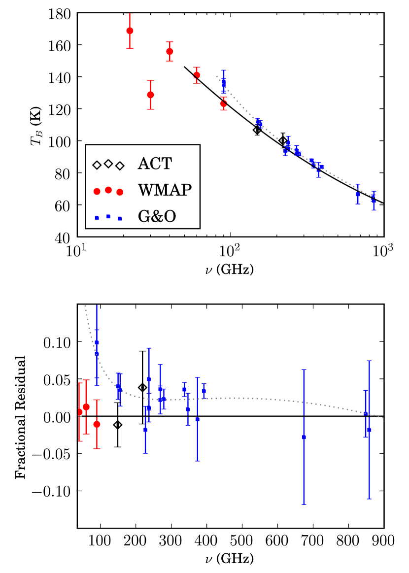
Figure 5.— Measurements of the Uranus brightness temperature from this work, Weiland et al. (2011, WMAP), and Griffin & Orton (1993, G&O). The G&O points include data from that work as well as Ulich (1981) and Orton et al. (1986). The dotted line shows the model of G&O. G&O data are calibrated to a Ulich-Wright hybrid model for Mars brightness that interpolates between 90 and 857 GHz and carries an estimated 5% systematic error. The solid line is our best-fit empirical model, using only the two highest frequency points from WMAP, the two ACT points, and the G&O points above 600 GHz.

5.2. Saturn

Measurements of the Saturn disk temperature are complicated by the presence of the rings, whose dust both obscures the main disk and radiates at a lower temperature. The ACT observations of Saturn span ring opening angles from -2 to 12 degrees and provide an opportunity to explore the separate contribution of these two components to the total effective brightness of the planet.

We follow closely the approach of Weiland et al. (2011, hereafter W11), who apply a two-parameter model in which the opacity and geometry of the rings are fixed, while the disk temperature and an effective temperature for the rings are free to vary. The ring dimensions and normal opacities are taken from Dunn et al. (2002). For each of the 148 GHz and 218 GHz arrays, we fit $T_{\rm disk}{}$ and $T_{\rm ring}{}$, which describe the mean disk temperature and mean effective brightness temperature of the rings (see W11 for the detailed definition), respectively.

The measurements of $\widehat{\alpha}{}$ and $\widehat{\beta}{}$ for each Saturn observation are converted to RJ temperatures, including corrections for PWV level and focus parameter, and with the CMB-based calibration applied. Because the scatter in the temperatures is not fully accounted for by the errors in the amplitude measurements and correction parameters, we combine observations made in single 15 to 30 day periods, taking the uncertainty in each combined measurement to be the error in the mean of the contributing data. As a result, a small number of temporally isolated observations are discarded. The binned data points, and the best fit model, are shown in Figure 6.

The fit of the W11 model includes a full accounting of the non-trivial correlations in the calibration uncertainty of the data points. The resulting models are good fits, with $\chi^{2}$ per degree of freedom of 7.6/5 (6.5/5) in the 148 GHz (218 GHz) array. The model fit parameters and uncertainties are presented in Table 5.

For comparison, we also fit a single temperature model to the binned Saturn data, finding poorer fits and mean temperatures that are 1–$\sigma$ less than the disk temperatures obtained in the full model. These temperatures and $\chi^{2}$ statistics are also presented in Table 5.

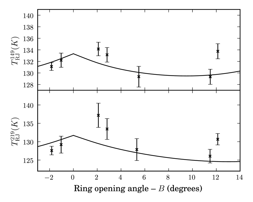
Figure 6.— Binned data and resulting best-fit two-component model of effective Saturn brightness vs. ring opening angle ($B$) relative to observer. The model is symmetric about $B=0$ by construction. As the absolute value of $B$ increases, the increased radiation from the rings and decreased flux from the obscured disk leads to a local minimum in the total effective brightness at $B\approx$ 9 ° (13 °) at 149 GHz (219 GHz). The model is fitted independently for each frequency band. Error bars correspond to the error in the mean of observations contributing to each point, but fits include additional error due to calibration, which is covariant within each season and in some cases between seasons. Approximate mean dates of observation are, from left to right: Nov/08, Dec/08, Jun/10, Apr/10, Dec/09, Dec/10, Dec/10. The sign convention is such that $B<0$ corresponds to negative values of the sub-Earth latitude.

In Figure 7 we show the ACT disk temperature measurements along with high precision results from W11 below 100 GHz and from Goldin et al. (1997, hereafter G97) between 170 and 700 GHz. The G97 measurements have statistical errors at the 2% level, but are calibrated with reference to the same Mars model used by G&O. We have applied a rough recalibration factor to the G97 measurements using the WMAP result (Weiland et al., 2011) that the Ulich (1981) model for Mars temperature is 5% high at 94 GHz. Our recalibration factor varies linearly with the log of frequency from 0.95 at 90 GHz to 1 at 857 GHz. With this calibration factor applied, the G97 measurement at 170 GHz and ACT measurements at 149 and 219 GHz are consistent with a flat spectrum over this frequency range. It is difficult to comment further on the continuum spectrum of Saturn based on the ACT and G97 data, due to the proximity of the high frequency G97 bands to PH₃ resonances (e.g., Weisstein & Serabyn, 1996).

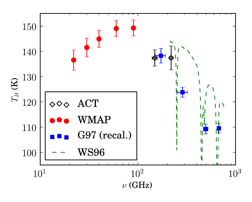
Figure 7.— Measurements of the Saturn disk brightness temperature from ACT, Weiland et al. (2011, WMAP), and Goldin et al. (1997, G97). Points from G97 have been recalibrated as described in the text. Frequency error bars on ACT and G97 points indicate bandwidth. Temperature error bars on G97 points do not include calibration uncertainty. The green dashed line is a spectral model from Weisstein & Serabyn (1996, WS96), which shows proximity of absorption features to G97 points.

6. Conclusion

We have described the reduction of ACT planet observations for the purposes of measuring and monitoring the telescope beam and gain parameters. The core of the beam has been well characterized by Saturn observations, and studies of point sources in the map have provided an empirical correction to account for pointing variance, alignment error, and slight changes in beam focus. Observations of Uranus have been used to measure and account for changes in system gain due to atmospheric water vapor and focus variation.

Based on hundreds of brightness measurements of Uranus, we have obtained precise measurements of the disk brightness temperature at 148 GHz and 218 GHz. In contrast to previous observations, our absolute calibration standard is the CMB blackbody. We have also obtained precise measurements of the Saturn disk temperature, in the context of a simple two-component model.

This work was supported by the U.S. National Science Foundation through awards AST-0408698 and AST-0965625 for the ACT project, as well as awards PHY-0855887 and PHY-1214379. Funding was also provided by Princeton University, the University of Pennsylvania, and a Canada Foundation for Innovation (CFI) award to UBC. ACT operates in the Parque Astronómico Atacama in northern Chile under the auspices of the Comisión Nacional de Investigación Científica y Tecnológica de Chile (CONICYT). Computations were performed on the GPC supercomputer at the SciNet HPC Consortium. SciNet is funded by the CFI under the auspices of Compute Canada, the Government of Ontario, the Ontario Research Fund – Research Excellence; and the University of Toronto.

References

- Archinal et al. (2011) Archinal, B. A., et al. 2011, Celestial Mechanics and Dynamical Astronomy, 109, 101
- Das et al. (2013) Das, S., et al. 2013, JCAP submitted (arXiv:1301.1037)
- Dunkley et al. (2013) Dunkley, J., et al. 2013, JCAP submitted (arXiv:1301.0776)
- Dunn et al. (2002) Dunn, D. E., Molnar, L. A., & Fix, J. D. 2002, Icarus, 160, 132
- Dünner et al. (2013) Dünner, R., Hasselfield, M., Marriage, T. A., Sievers, J., et al. 2013, ApJ, 762, 10
- Fowler et al. (2007) Fowler, J. W., et al. 2007, Appl. Opt., 46, 3444
- Goldin et al. (1997) Goldin, A. B., et al. 1997, ApJ, 488, L161
- Griffin & Orton (1993) Griffin, M. J., & Orton, G. S. 1993, Icarus, 105, 537
- Hajian et al. (2011) Hajian, A., et al. 2011, ApJ, 740, 86
- Hasselfield et al. (2013) Hasselfield, M., et al. 2013, JCAP submitted (arXiv:1301.0816)
- Hincks et al. (2010) Hincks, A. D., et al. 2010, ApJS, 191, 423
- Jarosik et al. (2011) Jarosik, N., et al. 2011, ApJS, 192, 14
- Klein & Hofstadter (2006) Klein, M. J., & Hofstadter, M. D. 2006, Icarus, 184, 170
- Kramer et al. (2008) Kramer, C., Moreno, R., & Greve, A. 2008, A&A, 482, 359
- Marriage (2006) Marriage, T. A. 2006, PhD thesis, Princeton University
- Marriage et al. (2011a) Marriage, T. A., et al. 2011a, ApJ, 731, 100
- Marriage et al. (2011b) —. 2011b, ApJ, 737, 61
- Orton et al. (1986) Orton, G. S., Griffin, M. J., Ade, P. A. R., Nolt, I. G., & Radostitz, J. V. 1986, Icarus, 67, 289
- Page et al. (2003) Page, L., et al. 2003, ApJS, 148, 39
- Pardo et al. (2001) Pardo, J. R., Cernicharo, J., & Serabyn, E. 2001, IEEE Transactions on Antennas and Propagation, 49, 1683
- Sayers et al. (2012) Sayers, J., Czakon, N. G., & Golwala, S. R. 2012, ApJ, 744, 169
- Sievers et al. (2013) Sievers, J. L., et al. 2013, JCAP submitted (arXiv:1301.0824)
- Sunyaev & Zel’dovich (1970) Sunyaev, R. A., & Zel’dovich, Y. B. 1970, Comments on Astrophysics and Space Physics, 2, 66
- Swetz et al. (2011) Swetz, D. S., et al. 2011, ApJS, 194, 41
- Tegmark (1997) Tegmark, M. 1997, ApJ, 480, L87
- Ulich (1981) Ulich, B. L. 1981, AJ, 86, 1619
- Weiland et al. (2011) Weiland, J. L., et al. 2011, ApJS, 192, 19
- Weisstein & Serabyn (1996) Weisstein, E. W., & Serabyn, E. 1996, Icarus, 123, 23
- White & Srednicki (1995) White, M., & Srednicki, M. 1995, ApJ, 443, 6
- Wright (1976) Wright, E. L. 1976, ApJ, 210, 250