Weighted estimation of the dependence function for an extreme-value distribution

Abstract

Bivariate extreme-value distributions have been used in modeling extremes in environmental sciences and risk management. An important issue is estimating the dependence function, such as the Pickands dependence function. Some estimators for the Pickands dependence function have been studied by assuming that the marginals are known. Recently, Genest and Segers [Ann. Statist. 37 (2009) 2990–3022] derived the asymptotic distributions of those proposed estimators with marginal distributions replaced by the empirical distributions. In this article, we propose a class of weighted estimators including those of Genest and Segers (2009) as special cases. We propose a jackknife empirical likelihood method for constructing confidence intervals for the Pickands dependence function, which avoids estimating the complicated asymptotic variance. A simulation study demonstrates the effectiveness of our proposed jackknife empirical likelihood method.

, and

1 Introduction

Let $(X_{11},X_{12}),\ldots,(X_{n1},X_{n2})$ be independent random pairs with common distribution function $F$ and continuous marginal distributions $F_{1}(x)=F(x,\infty)$ and $F_{2}(y)=F(\infty,y)$. Then the copula of $F$ is defined as

$$C(x,y)=P\bigl{(}F_{1}(X_{11})\leq x,F_{2}(X_{12})\leq y\bigr{)}.$$

When $C^{t}(u^{1/t},v^{1/t})=C(u,v)$ holds for all $u,v\in[0,1]$ and $t>0$, $C$ is called an extreme value copula and is determined by the Pickands dependence function, $A$, through the equation

$$C(u,v)=\exp\biggl{\{}\log(uv)A\biggl{(}\frac{\log(v)}{\log(uv)}\biggr{)}\biggr{\}}$$ (1)

for all $(u,v)\in(0,1]^{2}\setminus\{(1,1)\}$, where $A$ is a convex function and satisfies $\max(t,1-t)\leq A(t)\leq 1$ for all $0\leq t\leq 1$ (see Pickands [16] and Falk and Reiss [6]).

Write $Y_{ij}=-\log\{F_{j}(X_{ij})\}$ for $i=1,\ldots,n$, $j=1,2$ and

$$H_{n}(z)=\frac{1}{n}\sum_{i=1}^{n}I\biggl{(}\frac{Y_{i1}}{Y_{i1}+Y_{i2}}\leq z\biggr{)}.\vspace*{-2pt}$$

We denote $u\wedge v=\min(u,v)$ and $u\vee v=\max(u,v)$ throughout. Estimators for the Pickands dependence function $A(t)$ when the marginal distributions $F_{j},j=1,2$ are known have been proposed by Pickands [16], Deheuvels [5], Hall and Tajvidi [10], and Capéraà, Fougères and Genest [3], defined as

$$A^{P}(t) = \frac{n}{\sum_{i=1}^{n}\{Y_{i1}/t\}\wedge\{Y_{i2}/(1-t)\}},$$

$$A^{D}(t) = \frac{n}{\sum_{i=1}^{n}\{Y_{i1}/t\}\wedge\{Y_{i2}/(1-t)\}-t\sum_{i=1}^{n}Y_{i1}-(1-t)\sum_{i=1}^{n}Y_{i2}+n},$$

$$A^{\mathit{HT}}(t) = \frac{n}{\sum_{i=1}^{n}\{({nY_{i1}})/({t\sum_{j=1}^{n}Y_{j1}})\}\wedge\{{nY_{i2}}/{((1-t)\sum_{j=1}^{n}Y_{j2})}\}},$$

$$A^{\mathit{CFG}}(t) = \exp\biggl{\{}\lambda(t)\int_{0}^{t}\frac{H_{n}(z)-z}{z(1-z)}\,\mathrm{d}z-\bigl{(}1-\lambda(t)\bigr{)}\int_{t}^{1}\frac{H_{n}(z)-z}{z(1-z)}\,\mathrm{d}z\biggr{\}},\vspace*{-2pt}$$

respectively, where $\lambda(t)\in[0,1]$ is a weight function and $A^{P}(t)$ and $A^{D}(t)$ are corresponding limits when $t=0$ or $1$. When the marginal distributions are unknown, similar nonparametric estimators can be obtained by replacing the marginal distribution $F_{j}$ by the corresponding empirical distribution $F_{nj}(x)=\frac{1}{n}\sum_{i=1}^{n}I(X_{ij}\leq x)$ or $\hat{F}_{nj}(x)=\frac{1}{n+1}\sum_{i=1}^{n}I(X_{ij}\leq x).$ We denote these estimators as $\tilde{A}^{P}(t),\tilde{A}^{D}(t),\tilde{A}^{\mathit{HT}}(t)$ and $\tilde{A}^{\mathit{CFG}}(t)$. Recently, Genest and Segers [8] showed that $\tilde{A}^{P}(t),\tilde{A}^{D}(t)$ and $\tilde{A}^{\mathit{HT}}(t)$ have the same asymptotic distribution as

$$\hat{A}^{P}(t)=\frac{n}{\sum_{i=1}^{n}\{Z_{i1}/(1-t)\}\wedge\{Z_{i2}/t\}}\vspace*{-2pt}$$

and that $\tilde{A}^{\mathit{CFG}}(t)$ with $\lambda(t)=t$ has the same asymptotic distribution as

$$\hat{A}^{\mathit{CFG}}(t)=\exp\Biggl{\{}-\gamma-\frac{1}{n}\sum_{i=1}^{n}\bigl{(}Z_{i1}/(1-t)\bigr{)}\wedge(Z_{i2}/t)\Biggr{\}},\vspace*{-2pt}$$

where $\gamma=-\int_{0}^{\infty}\log(x)\mathrm{e}^{-x}\,\mathrm{d}x$ is the Euler constant and

$$Z_{ij}=-\log\{\hat{F}_{nj}(X_{ij})\}\qquad\mbox{for }i=1,\ldots,n,j=1,2.\vspace*{-2pt}$$

Moreover, Genest and Segers [8] derived the asymptotic distributions of $\hat{A}^{P}(t)$ and $\hat{A}^{\mathit{CFG}}(t)$ by noting the following important relationship:

$$\hat{A}^{P}(t)=\biggl{\{}\int_{0}^{1}u^{-1}\hat{C}_{n}(u^{1-t},u^{t})\,\mathrm{d}u\biggr{\}}^{-1}$$

and

$$\hat{A}^{\mathit{CFG}}(t)=\exp\biggl{(}-\gamma+\int_{0}^{1}\{\hat{C}_{n}(u^{1-t},u^{t})-I(u>\mathrm{e}^{-1})\}\{u\log(u)\}^{-1}\,\mathrm{d}u\biggr{)},\vspace*{-2pt}$$

where

$$\hat{C}_{n}(u,v)=\frac{1}{n}\sum_{i=1}^{n}I\bigl{(}\hat{F}_{n1}(X_{i1})\leq u,\hat{F}_{n2}(X_{i2})\leq v\bigr{)}.\vspace*{-2pt}$$

In this article, we propose a class of weighted estimators including $\hat{A}^{P}(t)$ and $\hat{A}^{\mathit{CFG}}(t)$ as special cases. We provide details in Section 2. In Section 3 we propose a jackknife empirical likelihood method to construct confidence intervals for the Pickands dependence function. Unlike the normal approximation method, this new method does not need to estimate any additional quantities, such as asymptotic variance. In Section 4 we report a simulation study conducted to examine the finite sample behavior of the proposed jackknife empirical likelihood method. We provide proofs in Section 5.

2 Weighted estimation

It follows from (1) that

$$C(u^{1-t},u^{t})=u^{A(t)}\qquad\mbox{for all }u\in[0,1]\mbox{ and all }t\in[0,1],\vspace*{-2pt}$$ (2)

which motivates the estimation of $A(t)$ by minimizing the following weighted distance with respect to $\alpha\geq 0$:

$$\int_{0}^{1}\{\hat{C}_{n}(u^{1-t},u^{t})-u^{\alpha}\}^{2}\bar{\lambda}(u,t)\,\mathrm{d}u,\vspace*{-2pt}$$

where $\bar{\lambda}(u,t)\geq 0$ is a weight function. Under some regularity conditions, the foregoing estimator is the solution of $\alpha$ to the equation

$$\int_{0}^{1}\{\hat{C}_{n}(u^{1-t},u^{t})-u^{\alpha}\}u^{\alpha}\{-\log(u)\}\bar{\lambda}(u,t)\,\mathrm{d}u=0\vspace*{-2pt}$$

for $\alpha>0$. This is a special case of the proposed M-estimators and Z-estimators of Bücher, Dette and Volgushev [2]. Noting that $u^{\alpha}(-\log u)\bar{\lambda}(u,t)=C(u^{1-t},u^{t})(-\log u)\bar{\lambda}(u,t)$ and $\bar{\lambda}(u,t)$ is any weight function, we propose treating $C(u^{1-t},u^{t})(-\log u)\bar{\lambda}(u,t)$ as a new weight function. This leads us to estimate $A(t)$ by solving the following equation with respect to $\alpha\geq 0$:

$$\int_{0}^{1}\{\hat{C}_{n}(u^{1-t},u^{t})-u^{\alpha}\}\lambda(u,t)\,\mathrm{d}u=0,\vspace*{-2pt}$$ (3)

where $\lambda(u,t)\geq 0$ is a new weight function. We denote this new estimator by $\hat{A}^{w}_{n}(t;\lambda)$. When $\lambda(u,t)$ is taken as $u^{-1}$ or $\{-u\log(u)\}^{-1}$, $\hat{A}^{w}_{n}(t;\lambda)$ becomes $\hat{A}^{P}(t)$ or $\hat{A}^{\mathit{CFG}}(t)$. Thus, the foregoing class of estimators includes the known estimators in the literature as special cases.

Write $g(\alpha)=\int_{0}^{1}\{\hat{C}_{n}(u^{1-t},u^{t})-u^{\alpha}\}\lambda(u,t)\,\mathrm{d}u.$ Because $u^{\alpha}$ is a decreasing function of $\alpha$ for each fixed $u\in[0,1]$, $g(\alpha)$ is an increasing function of $\alpha$ for each fixed $t$. Moreover, $g(0)<0$ and $g(\infty)>0$ when $n$ is sufficiently large. Thus, (3) has a unique solution $\hat{A}^{w}_{n}(t;\lambda)$ for each large $n$ and $t\in[0,1]$. Note that this unique solution might not satisfy that $\max(t,1-t)\leq\hat{A}^{w}_{n}(t;\lambda)\leq 1$ and $\hat{A}^{w}_{n}(0;\lambda)=\hat{A}^{w}_{n}(1;\lambda)=1$.

Let $W(u,v)$ denote a tight Gaussian process with mean 0, covariance

$$E\{W(u_{1},v_{1})W(u_{2},v_{2})\}=C(u_{1}\wedge u_{2},v_{1}\wedge v_{2})-C(u_{1},v_{1})C(u_{2},v_{2}),$$

and $W(u,0)=W(0,v)=W(1,1)=0$ for all $u,v\in[0,1]$. The asymptotic distribution for the proposed estimator $\hat{A}^{w}_{n}(t;\lambda)$ is given in the following theorem.

Theorem 2.1

Suppose that $\frac{\partial^{2}}{\partial u^{2}}C(u,v)$, $\frac{\partial^{2}}{\partial v^{2}}C(u,v)$ and $\frac{\partial^{2}}{\partial u\,\partial v}C(u,v)$ are defined and continuous on the sets ${\cal F}_{1}=\{(u,v)\colon\ 0<u<1\mbox{ and }0\leq v\leq 1\}$, ${\cal F}_{2}=\{(u,v)\colon\ 0\leq u\leq 1,0<v<1\}$ and ${\cal F}_{3}=\{(u,v)\colon\ 0<u<1,0<v<1\}$, respectively. Also assume that for each fixed $t\in[0,1]$ the function $\lambda(u,t)\geq 0$ is continuous and not equal to 0 as a function of $u\in(0,1)$. Furthermore, assume that

$$\cases{\displaystyle\biggl{|}\frac{\partial^{2}}{\partial u^{2}}C(u,v)\biggr{|}\leq\frac{M}{u(1-u)}&\quad for $(u,v)\in{\cal F}_{1}$,\vspace*{2pt}\cr\displaystyle\biggl{|}\frac{\partial^{2}}{\partial v^{2}}C(u,v)\biggr{|}\leq\frac{M}{v(1-v)}&\quad for $(u,v)\in{\cal F}_{2}$,\vspace*{2pt}\cr\displaystyle\biggl{|}\frac{\partial^{2}}{\partial u\,\partial v}C(u,v)\biggr{|}\leq\frac{M}{u(1-u)}\wedge\frac{M}{v(1-v)}&\quad for $(u,v)\in{\cal F}_{3}$}$$

for some constant $M>0$, $A^{\prime}(t)$ is continuous on $[0,1]$, and there exist $\delta_{1}>0$ and $\delta_{2}\in[0,1/2)$ such that

$$\cases{\displaystyle\sup_{0\leq t\leq 1}\sqrt{n}\int_{0}^{(n+1)^{-1/((1-t)\vee t)}}u^{1/2}\lambda(u,t)\,\mathrm{d}u\to 0,\vspace*{2pt}\cr\displaystyle\sup_{0\leq t\leq 1}\sqrt{n}\int_{({n}/{(n+1)})^{1/((1-t)\vee t)}}^{1}(1-u)\lambda(u,t)\,\mathrm{d}u\to 0,\vspace*{2pt}\cr\displaystyle\sup_{0\leq t\leq 1}n^{-1/4+\delta_{1}}\int_{(n+1)^{-1/((1-t)\vee t)}}^{({n}/{(n+1)})^{1/((1-t)\vee t)}}\lambda(u,t)\,\mathrm{d}u\to 0,\vspace*{2pt}\cr\displaystyle\sup_{0\leq t\leq 1}\int_{0}^{1}\bigl{\{}u^{(1-t)\vee t}\bigl{(}1-u^{(1-t)\vee t}\bigr{)}\bigr{\}}^{\delta_{2}}\lambda(u,t)\,\mathrm{d}u<\infty,\vspace*{2pt}\cr\displaystyle\sup_{0\leq t\leq 1}\int_{0}^{1}u^{(1-t)\vee t-(1-t)}u^{(1-t)\delta_{2}}(1-u^{1-t})^{\delta_{2}}\lambda(u,t)\,\mathrm{d}u<\infty,\vspace*{2pt}\cr\displaystyle\sup_{0\leq t\leq 1}\int_{0}^{1}u^{(1-t)\vee t-t}u^{t\delta_{2}}(1-u^{t})^{\delta_{2}}\lambda(u,t)\,\mathrm{d}u<\infty,\vspace*{2pt}\cr\displaystyle\sup_{0\leq t\leq 1}\int_{1/2}^{1}(-\log u)\lambda(u,t)\,\mathrm{d}t<\infty.}$$ (4)

Then as $n\to\infty$, $\sup_{0\leq t\leq 1}|\hat{A}^{w}_{n}(t;\lambda)-A(t)|=\mathrm{o}_{p}(1)$. Moreover, suppose that $\lambda(u,t)$ is continuous in $(0,1)\times[0,1]$ and

$$|\lambda(u,t_{1})-\lambda(u,t_{2})|\leq|t_{1}-t_{2}|^{\delta_{0}}\lambda_{0}(u),\qquad t_{1},t_{2}\in[0,1],u\in(0,1)$$

for some constant $\delta_{0}>0$ and function $\lambda_{0}(u),u\in(0,1)$, where $\lambda_{0}(u)$ satisfies that

$$\int^{1/2}_{0}u^{\alpha}\lambda_{0}(u)\,\mathrm{d}u<\infty,\qquad\int^{1}_{1/2}(1-u^{\alpha})\lambda_{0}(u)\,\mathrm{d}u<\infty$$

for all $\alpha>0$. Then, as $n\rightarrow\infty$, $\sqrt{n}\{\hat{A}^{w}_{n}(t;\lambda)-A(t)\}$ converges to $B(t)$ in $C([0,1])$, where

$$B(t) = \biggl{\{}\int_{0}^{1}C(u^{1-t},u^{t})\lambda(u,t)\log(u)\,\mathrm{d}u\biggr{\}}^{-1}$$

$${}\times\int_{0}^{1}\{W(u^{1-t},u^{t})-C_{1}(u^{1-t},u^{t})W(u^{1-t},1)-C_{2}(u^{1-t},u^{t})W(1,u^{t})\}\lambda(u,t)\,\mathrm{d}u,$$

$C_{1}(u,v)=\frac{\partial}{\partial u}C(u,v)$ and $C_{2}(u,v)=\frac{\partial}{\partial v}C(u,v)$.

Remark 2.0.

Theorem 2.1 still holds when condition (4) is replaced by

$$\cases{\displaystyle\sup_{0\leq t\leq 1}\sqrt{n}\int_{0}^{(n+1)^{-2}}u^{1/2}\lambda(u,t)\,\mathrm{d}u\to 0,\vspace*{2pt}\cr\displaystyle\sup_{0\leq t\leq 1}\sqrt{n}\int_{({n}/{(n+1)})^{2}}^{1}(1-u)\lambda(u,t)\,\mathrm{d}u\to 0,\vspace*{2pt}\cr\displaystyle\sup_{0\leq t\leq 1}n^{-1/4+\delta_{1}}\int^{({n}/{(n+1)})^{2}}_{(n+1)^{-2}}\lambda(u,t)\,\mathrm{d}u\to 0,\vspace*{2pt}\cr\displaystyle\sup_{0\leq t\leq 1}\int_{0}^{1}u^{\delta_{2}/2}(1-u)^{\delta_{2}}\lambda(u,t)\,\mathrm{d}u<\infty}$$

for some $\delta_{1}>0$ and $\delta_{2}\in[0,1/2)$. This follows from the proof of Theorem 2.1 by replacing $\int_{0}^{(n+1)^{-1/((1-t)\vee t)}}$, $\int_{(n+1)^{-1/((1-t)\vee t)}}^{({n}/{(n+1)})^{1/((1-t)\vee t)}}$ and $\int_{({n}/{(n+1)})^{1/((1-t)\vee t)}}^{1}$ in (5) by $\int_{0}^{(n+1)^{-2}}$, $\int_{(n+1)^{-2}}^{({n}/{(n+1)})^{2}}$ and $\int_{({n}/{(n+1)})^{2}}^{1}$, respectively.

Remark 2.0.

A common approach to choosing $\lambda(u,t)$ is to minimize the asymptotic variance of $\hat{A}^{w}_{n}(t;\lambda)$. This is difficult to do analytically. Linear combinations of some known estimators can be considered instead. For example, suppose that the weight functions $\lambda_{1}(u),\ldots,\lambda_{q}(u)$ give the corresponding estimators $\hat{A}^{w}_{n,1}(t),\ldots,\hat{A}^{w}_{n,q}(t)$. Define the class of new weight functions as

$${\cal F}_{0}=\Biggl{\{}\lambda(u,t)\colon\ \lambda(u,t)=\sum_{i=1}^{q}a_{i}(t)\lambda_{i}(u),a_{1}(t)\geq 0,\ldots,a_{q}(t)\geq 0,\sum_{i=1}^{q}a_{i}(t)=1\Biggr{\}}.$$

Then one can choose $a_{i}^{\prime}s$ to minimize the asymptotic variance of $\hat{A}^{w}_{n}(t;\lambda)$ in this class ${\cal F}_{0}$, which results in explicit formulas for $a_{i}^{\prime}s$.

Assume that $\lambda(u,t)=u^{-1}(-\log u)^{-q(t)}$ for some $q(t)\in[0,1]$. Then $\hat{A}^{P}(t)$ and $\hat{A}^{\mathit{CFG}}(t)$ correspond to $q(t)=0$ and $q(t)=1$, respectively. When $q(t)<1$, we can write

$$\int_{0}^{1}\{\hat{C}_{n}(u^{1-t},u^{t})-u^{\theta}\}\lambda(u,t)\,\mathrm{d}u$$

$$\quad=-\frac{1}{1-q(t)}\int_{0}^{1}\{\hat{C}_{n}(u^{1-t},u^{t})-u^{\theta}\}\,\mathrm{d}(-\log u)^{1-q(t)}$$

$$\quad=\frac{1}{1-q(t)}\int_{0}^{1}(-\log u)^{1-q(t)}\,\mathrm{d}\bigl{(}\hat{C}_{n}(u^{1-t},u^{t})-u^{\theta}\bigr{)}$$

$$\quad=\frac{1}{1-q(t)}\int_{0}^{1}(-\log u)^{1-q(t)}\,\mathrm{d}\hat{C}_{n}(u^{1-t},u^{t})-\frac{\theta^{q(t)-1}}{1-q(t)}\int^{\infty}_{0}u^{1-q}\mathrm{e}^{-u}\,\mathrm{d}u$$

$$\quad=\frac{1}{1-q(t)}\Biggl{\{}\frac{1}{n}\sum_{i=1}^{n}\biggl{\{}\frac{Z_{i1}}{1-t}\wedge\frac{Z_{i2}}{t}\biggr{\}}^{1-q(t)}-\theta^{q(t)-1}\Gamma\bigl{(}2-q(t)\bigr{)}\Biggr{\}},$$

where the $Z_{ij}^{\prime}s$ are as defined in Section 1. Thus,

$$\hat{A}^{w}_{n}(t;\lambda)=\exp\Biggl{\{}-\Biggl{(}\log\Biggl{(}\frac{1}{n}\sum_{i=1}^{n}\biggl{(}\frac{Z_{i1}}{1-t}\wedge\frac{Z_{i2}}{t}\biggr{)}^{1-q(t)}\Biggr{)}-\log\Gamma\bigl{(}2-q(t)\bigr{)}\Biggr{)}\Big{/}\bigl{(}1-q(t)\bigr{)}\Biggr{\}}$$

for $0\leq q(t)\leq 1$. Note that when $q(t)=1$, the foregoing expression is defined as the limit, which becomes the same as $\hat{A}^{\mathit{CFG}}(t)$. In particular, we propose to choose $q(t)=\min\{\hat{A}^{\mathit{CFG}}(t),1\}$ and denote the resulting estimator by $\hat{A}^{w}_{n}(t).$ To compare this new estimator with $\hat{A}^{\mathit{CFG}}(t)$, we draw $1000$ random samples with size $n=100,1000,5000$ from a Gumbel copula with $A(t)=\{t^{\theta}+(1-t)^{\theta}\}^{1/\theta}$, a Hüsler–Reiss copula with $A(t)=(1-t)\Phi(\theta+\frac{1}{2\theta}\log\frac{1-t}{t})+t\Phi(\theta+\frac{1}{2\theta}\log\frac{t}{1-t})$, and a Tawn copula with $A(t)=1-\theta t+\theta t^{2}$, where $\Phi(x)$ denotes the distribution function of $N(0,1)$. Figure 1 plots the ratios of the mean squared error of $\hat{A}^{w}_{n}(t)$ to the mean squared error of $\hat{A}^{\mathit{CFG}}(t)$ for $t=0.1,0.2,\ldots,0.9$, and shows that the new estimator has a smaller mean squared error than $\hat{A}^{\mathit{CFG}}(t)$ in all of the cases considered.

3 Jackknife empirical likelihood method

In this section, we consider interval estimation for the Pickands dependence function $A(t)$, which plays an important role in risk management since one may be concerned with interval estimation for $C(u,v)$ at some particular values of $u$ and $v$. Note that an interval for $A(t)$ can be easily transformed to an interval for a monotone function of $A(t)$. Moreover, these two intervals have the same coverage probability, but different interval lengths. Because the upper tail dependence coefficient can be written as a monotone function of $A(1/2)$, an interval can be constructed via an interval for $A(1/2)$.

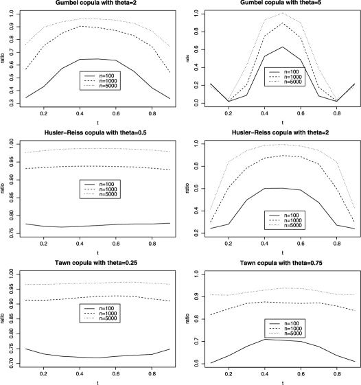
Figure 1: Ratios of the mean squared error of the new estimator $\hat{A}^{w}_{n}(t)$ to that of $\hat{A}^{\mathit{CFG}}(t)$ for $t=0.1,0.2,\ldots,0.9$.

An obvious approach to constructing an interval for $A(t)$ is to use the normal approximation method based on any one of the estimators for $A(t)$. Because the asymptotic distribution of any one of the estimators for $A(t)$ depends on its derivative $A^{\prime}(t)$, the normal approximation method requires estimating $A^{\prime}(t)$ first. In an alternative approach to constructing confidence intervals, the empirical likelihood method has been extended and applied in various fields since Owen [13, 14] introduced it for construction of a confidence interval/region for a mean. (See Owen [15] for an overview.) An important feature of the empirical likelihood method is its property of self-studentization, which avoids estimating the asymptotic variance explicitly. A general approach to formulating the empirical likelihood function is based on estimating equations, as in Qin and Lawless [17].

Because our proposed weighted estimator is defined as the solution to equation (3), the method of Qin and Lawless [17] may be applied directly by defining the empirical likelihood function as

$$\sup\Biggl{\{}\prod_{i=1}^{n}(np_{i})\colon\ p_{1}\geq 0,\ldots,p_{n}\geq 0,\sum_{i=1}^{n}p_{i}=1,$$

$$\hphantom{\sup\Biggl{\{}}\sum_{i=1}^{n}p_{i}\int_{0}^{1}\bigl{\{}I\bigl{(}\hat{F}_{n1}(X_{i1})\leq u^{1-t},\hat{F}_{n2}(X_{i2})\leq u^{t}\bigr{)}-u^{\theta}\bigr{\}}\lambda(u,t)\,\mathrm{d}u=0\Biggr{\}}.$$

However, this method cannot catch the variation introduced by the marginal empirical distributions. In other words, the limit is no longer a chi-squared distribution. In general, the nonlinear functional must be linearized by introducing some link variables before the profile empirical likelihood method is used. (See Chen, Peng and Zhao [4] for details on applying the profile empirical likelihood method to copulas.) Unfortunately, this linearization idea is not applicable to the estimation of $A(t)$. Recently, Jing, Yuan and Zhou [11] proposed a so-called “jackknife empirical likelihood” method to construct confidence intervals for U-statistics. More specifically, these authors proposed applying the empirical likelihood method to jackknife samples, which could result in a chi-squared limit. Motivated by Gong, Peng and Qi [9]’s study of the use of a smoothed jackknife empirical likelihood method to construct a confidence interval for a receiver operating characteristic curve, one needs to work with a smoothed version of the left-hand side of (3). The reason for smoothing is to separate marginals from the copula estimator when expanding the jackknife empirical likelihood ratio. In this work, we used the smoothed empirical copula of Fermanian, Radulović and Wegkamp [7], defined as

$$\hat{C}_{n}^{s}(u^{1-t},u^{t})=\frac{1}{n}\sum_{i=1}^{n}K\biggl{(}\frac{u-\hat{F}_{n1}^{1/(1-t)}(X_{i1})}{h}\biggr{)}K\biggl{(}\frac{u-\hat{F}_{n2}^{1/t}(X_{i2})}{h}\biggr{)},$$

where $K(x)=\int_{-\infty}^{x}k(s)\,\mathrm{d}s$, $k$ is a symmetric density function with support $[-1,1]$, and $h=h(n)>0$ is a bandwidth. Based on this smoothed estimation, a jackknife empirical likelihood function can be constructed as follows. Put $\hat{F}_{nj,-i}(x)=\frac{1}{n}\sum_{l=1,l\neq i}^{n}I(X_{lj}\leq x)$ for $j=1,2$ and $i=1,\ldots,n$,

$$\hat{C}_{n,-i}^{s}(u^{1-t},u^{t})=\frac{1}{n-1}\sum_{j=1,j\neq i}^{n}K\biggl{(}\frac{u-\hat{F}_{n1,-i}^{1/(1-t)}(X_{j1})}{h}\biggr{)}K\biggl{(}\frac{u-\hat{F}_{n2,-i}^{1/t}(X_{j2})}{h}\biggr{)}$$

for $i=1,\ldots,n$, and define the jackknife sample as

$$\hat{V}_{i}(u,t)=n\hat{C}_{n}^{s}(u^{1-t},u^{t})-(n-1)\hat{C}_{n,-i}^{s}(u^{1-t},u^{t})$$

for $i=1,\ldots,n$.

We next apply the empirical likelihood method based on estimating equations of Qin and Lawless [17] to the foregoing jackknife sample. This gives the jackknife empirical likelihood function for $\theta=A(t)$ as

$$L(\theta) = \sup\Biggl{\{}\prod_{i=1}^{n}(np_{i})\colon\ p_{1}\geq 0,\ldots,p_{n}\geq 0,\sum_{i=1}^{n}p_{i}=1,$$

$$\hphantom{\sup\Biggl{\{}}\sum_{i=1}^{n}p_{i}\int_{a_{n}}^{1-b_{n}}\{\hat{V}_{i}(u,t)-u^{\theta}\}\lambda(u,t)\,\mathrm{d}u=0\Biggr{\}},$$

where $a_{n}>0$ and $b_{n}>0$. Note that we use $\int_{a_{n}}^{1-b_{n}}$ instead of $\int_{0}^{1}$ in defining the foregoing jackknife empirical likelihood function, to control the bias term and allow the possibility of $\lambda(0,t)=\infty$ and $\lambda(1,t)=\infty$.

By the standard Lagrange multiplier technique, we obtain the log jackknife empirical likelihood ratio as

$$l(\theta)=-2\log L(\theta)=2\sum_{i=1}^{n}\log\{1+\beta Q_{i}(\theta)\},$$

where

$$Q_{i}(\theta)=\int_{a_{n}}^{1-b_{n}}\{\hat{V}_{i}(u,t)-u^{\theta}\}\lambda(u,t)\,\mathrm{d}u$$

and $\beta=\beta(\theta)$ satisfies

$$\frac{1}{n}\sum_{i=1}^{n}\frac{Q_{i}(\theta)}{1+\beta Q_{i}(\theta)}=0.$$ (5)

Theorem 3.1

Suppose that $\frac{\partial^{2}}{\partial u^{2}}C(u,v)$, $\frac{\partial^{2}}{\partial v^{2}}C(u,v)$ and $\frac{\partial^{2}}{\partial u\,\partial v}C(u,v)$ are defined and continuous on the set ${\cal F}_{3}=\{(u,v),0<u<1\mbox{ and }0<v<1\}$ and

$$\biggl{|}\frac{\partial^{2}}{\partial u^{2}}C(u,v)\biggr{|} \leq \frac{M}{u(1-u)},\qquad\biggl{|}\frac{\partial^{2}}{\partial v^{2}}C(u,v)\biggr{|}\leq\frac{M}{v(1-v)},$$

$$\biggl{|}\frac{\partial^{2}}{\partial u\,\partial v}C(u,v)\biggr{|} \leq \frac{M}{u(1-u)}\wedge\frac{M}{v(1-v)}$$

for $(u,v)\in{\cal F}_{3}$ and some constant $M>0$. Let $t$ denote a fixed point in $(0,1)$. Assume that the function $\lambda(u,t)\geq 0$ is continuous and not identical to 0 as a function of $u\in(0,1)$, $A^{\prime}(s)$ is continuous at $s=t$, and

$$\cases{\displaystyle h=h(n)\to 0,\qquad nh\to\infty,\vspace*{2pt}\cr\displaystyle a_{n}\to 0,\qquad b_{n}\to 0,\qquad h/a_{n}\to 0,\qquad h/b_{n}\to 0,\vspace*{2pt}\cr\displaystyle n^{-1/4+\delta_{1}}\int_{a_{n}}^{1-b_{n}}\lambda(u,t)\,\mathrm{d}u\to 0\qquad\mbox{for some }\delta_{1}>0,\vspace*{2pt}\cr\displaystyle\int_{0}^{1}u^{\delta_{2}}(1-u^{\delta_{2}})\lambda(u,t)\,\mathrm{d}u<\infty\qquad\mbox{for some }\delta_{2}\in[0,1/2),\vspace*{2pt}\cr\displaystyle\sqrt{n}h^{2}\int_{a_{n}}^{1-b_{n}}u^{-3/2}\lambda(u,t)\,\mathrm{d}u\to 0,\vspace*{2pt}\cr\displaystyle\sqrt{n}h^{2}\int_{a_{n}}^{1-b_{n}}\{\log u\}^{-1}u^{-3/2}\lambda(u,t)\,\mathrm{d}u\to 0,\vspace*{2pt}\cr\displaystyle\frac{1}{\sqrt{n}h}\int_{a_{n}}^{1-b_{n}}u^{-1}\lambda(u,t)\,\mathrm{d}u\to 0,\vspace*{2pt}\cr\displaystyle n^{-3/2}\int_{a_{n}}^{1-b_{n}}u^{-2}\lambda(u,t)\,\mathrm{d}u\to 0}$$ (6)

as $n\to\infty$. Then $l(A_{0}(t))\stackrel{{\scriptstyle d}}{{\to}}\chi^{2}(1)$ as $n\to\infty$, where $A_{0}(t)$ denotes the true value of $A(t)$.

For any fixed $t\in(0,1)$, based on the foregoing theorem, a jackknife empirical likelihood confidence interval for $A_{0}(t)$ with level $\gamma_{0}$ can be constructed as

$$I_{\gamma_{0}}(t)=\{\theta\colon\ l(\theta)\leq\chi^{2}_{\gamma_{0}}\},$$

where $\chi^{2}_{\gamma_{0}}$ is the $\gamma_{0}$ quantile of $\chi^{2}(1)$, as follows:

Remark 3.0.

(i) When $\lambda(u,t)=\{-u\log u\}^{-1}$, we have $\sup_{0\leq u\leq 1}\lambda(u,t)=\infty$. We can choose

$$a_{n}=d_{1}n^{-a},\qquad b_{n}=d_{2}n^{-b},\qquad h=d_{3}n^{-1/3}$$

for some $d_{1},d_{2},d_{3}>0$, $0<a<1/9$, and $0<b<1/6$. (

• iii)]

• When $\sup_{0\leq u\leq 1}\lambda(u,t)<\infty$, we can choose

  $$a_{n}=d_{1}n^{-a},\qquad b_{n}=d_{2}n^{-b},\qquad h=d_{3}n^{-1/3}$$

  for some $d_{1},d_{2},d_{3}>0,b>0$, and $0<a<1/3$. Here we fix the rate for $h$ because the optimal rate for the bandwidth in smoothing distribution estimation is $n^{-1/3}$.

• Theorem 3.1 still holds when $a_{n}\to a\in(0,1/2)$ and $b_{n}\to b\in(0,1/2]$ as $n\to\infty$.

4 Simulation study

In this section we examine the finite-sample behavior of the proposed jackknife empirical likelihood method based on $\lambda(u,t)=u^{-1}(-\log u)^{-\min\{\hat{A}^{\mathit{CFG}}(t),1\}}$ in terms of coverage probability and compare it with the method based on the asymptotic distribution of $\hat{A}^{\mathit{CFG}}(t)$. For computing the coverage probability of the proposed jackknife empirical likelihood method, we choose $k(x)=\frac{15}{16}(1-x^{2})^{2}I(|x|\leq 1)$, $h=0.5n^{-1/3}$, $a_{n}=b_{n}=0.1$, $\lambda(u,t)=u^{-1}(-\log u)^{-\min\{\hat{A}^{\mathit{CFG}}(t),1\}}$ and use the R package “emplik” (see Zhou [19]). To compute the confidence interval based on the asymptotic distribution of $\hat{A}^{\mathit{CFG}}(t)$, we use the multiplier method proposed by Kojadinovic and Yan [12]. More specifically, we use eq. (7) of Kojadinovic and Yan [12], with $N=500$ and $\{Z_{i}^{(k)}\colon\ i=1,\ldots,n,k=1,\ldots,N\}$ as independent random variables from $N(0,1)$, to calculate the critical points of the asymptotic distribution of $\sqrt{n}\{\hat{A}^{\mathit{CFG}}(t)-A(t)\}$. We do not use a larger $N$, because this multiplier method is computationally intensive. A comparison study on bootstrap approximations has been reported by Bücher and Dette [1].

Table 1: Empirical coverage probabilities are reported for the proposed jackknife empirical likelihood confidence interval (JELCI) based on $\lambda(u,t)=u^{-1}(-\log u)^{-\min\{\hat{A}^{\mathit{CFG}}(t),1\}}$, and the confidence interval based on the multiplier method for $\hat{A}^{\mathit{CFG}}(t)$ (MCI) with nominal levels $0.9$ and $0.95$

	Level 0.9	Level 0.9	Level 0.95	Level 0.95
$(n,t,\mbox{Copula},\theta)$	JELCI	MCI	JELCI	MCI
$(100,0.1,\mbox{Gumbel},2)$	0.604	0.276	0.639	0.366
$(100,0.1,\mbox{H\"{u}sler-Reiss},0.5)$	0.845	0.566	0.899	0.655
$(100,0.1,\mbox{Tawn},0.25)$	0.817	0.571	0.872	0.670
$(100,0.5,\mbox{Gumbel},2)$	0.871	0.722	0.941	0.784
$(100,0.5,\mbox{H\"{u}sler-Reiss},0.5)$	0.888	0.715	0.941	0.802
$(100,0.5,\mbox{Tawn},0.25)$	0.886	0.750	0.941	0.825
$(100,0.8,\mbox{Gumbel},2)$	0.841	0.531	0.889	0.599
$(100,0.8,\mbox{H\"{u}sler-Reiss},0.5)$	0.889	0.646	0.947	0.758
$(100,0.8,\mbox{Tawn},0.25)$	0.884	0.677	0.938	0.758
$(1000,0.1,\mbox{Gumbel},2)$	0.888	0.655	0.935	0.740
$(1000,0.1,\mbox{H\"{u}sler-Reiss},0.5)$	0.892	0.813	0.942	0.883
$(1000,0.1,\mbox{Tawn},0.25)$	0.900	0.820	0.957	0.891

We draw $1000$ random samples with size $n=100,1000$ from the Gumbel copula, the Hüsler–Reiss copula, and the Tawn copula with Pickands dependence functions specified at the end of Section 2. Table 1 reports the coverage probabilities at levels $0.9$ and $0.95$ for $t=0.1,0.5,0.8$. These show that (i) the proposed jackknife empirical likelihood method gives much more accurate coverage probabilities than the multiplier method based on the asymptotic distribution of $\hat{A}^{\mathit{CFG}}(t)$, and (ii) our proposed jackknife empirical likelihood method performs poorly for the boundary case $t=0.1$ when $n=100$, but its performance improves as $n$ becomes large.

5 Proofs

Proof of Theorem 2.1 Define

$$\alpha_{n}(u,v)=\sqrt{n}\Biggl{\{}\frac{1}{n}\sum_{i=1}^{n}I\bigl{(}F_{1}(X_{i1})\leq u,F_{2}(X_{i2})\leq v\bigr{)}-C(u,v)\Biggr{\}}.$$

Then, from Proposition 4.2 of Segers [18] and Theorem G.1 of Genest and Segers [8], it follows that

$$\sup_{0\leq u,v\leq 1}\bigl{|}\sqrt{n}\{\hat{C}_{n}(u,v)-C(u,v)\}-\alpha_{n}(u,v)+C_{1}(u,v)\alpha_{n}(u,1)+C_{2}(u,v)\alpha_{n}(1,v)\bigr{|}$$

$$\quad=\mathrm{O}(n^{-1/4}(\log n)^{1/2}(\log\log n))\qquad\mbox{a.s.}$$

and

$$\frac{\alpha_{n}(u,v)}{(u\wedge v)^{\delta}(1-u\wedge v)^{\delta}}\stackrel{{\scriptstyle D}}{{\to}}\frac{W(u,v)}{(u\wedge v)^{\delta}(1-u\wedge v)^{\delta}}$$

in the space $l^{\infty}([0,1]^{2})$ of bounded, real-valued functions on $[0,1]^{2}$ for any $\delta\in[0,1/2)$, where $W$ is defined before Theorem 2.1. By the Skorohod construction, there exists a probability space carrying $\hat{C}_{n}^{*},\alpha_{n}^{*},W^{*}$ such that

$$(\hat{C}_{n}^{*},\alpha_{n}^{*})\stackrel{{\scriptstyle d}}{{=}}(\hat{C}_{n},\alpha_{n}),\qquad W^{*}\stackrel{{\scriptstyle d}}{{=}}W,\vspace*{-16pt}$$ (7)

$$\sup_{0\leq u,v\leq 1}\bigl{|}\sqrt{n}\{\hat{C}_{n}^{*}(u,v)-C(u,v)\}-\alpha_{n}^{*}(u,v)+C_{1}(u,v)\alpha_{n}^{*}(u,1)+C_{2}(u,v)\alpha_{n}^{*}(1,v)\bigr{|}$$

(8)

$$\quad=\mathrm{O}(n^{-1/4}(\log n)^{1/2}(\log\log n))\qquad\mbox{a.s.}$$

and

$$\sup_{0\leq u,v\leq 1}\biggl{|}\frac{\alpha_{n}^{*}(u,v)}{(u\wedge v)^{\delta}(1-u\wedge v)^{\delta}}-\frac{W^{*}(u,v)}{(u\wedge v)^{\delta}(1-u\wedge v)^{\delta}}\biggr{|}=\mathrm{o}_{p}(1).$$ (9)

Let $\hat{A}^{w*}_{n}(t;\lambda)$ denote the solution to

$$\int_{0}^{1}\{\hat{C}_{n}^{*}(u^{1-t},u^{t})-u^{\alpha}\}\lambda(u,t)\,\mathrm{d}u=0.$$

Then (7) implies that

$$\{\hat{A}^{w*}_{n}(t;\lambda)\colon\ 0\leq t\leq 1\}\stackrel{{\scriptstyle d}}{{=}}\{\hat{A}^{w}_{n}(t;\lambda)\colon\ 0\leq t\leq 1\}.$$ (10)

Write

$$\int_{0}^{1}\bigl{\{}\hat{C}_{n}^{*}(u^{1-t},u^{t})-u^{A(t)}\bigr{\}}\lambda(u,t)\,\mathrm{d}u$$

$$\quad=\int_{0}^{(n+1)^{-1/((1-t)\vee t)}}\bigl{\{}-u^{A(t)}\bigr{\}}\lambda(u,t)\,\mathrm{d}u$$

$$\qquad{}+\int_{(n+1)^{-1/((1-t)\vee t)}}^{({n}/{(n+1)})^{1/((1-t)\vee t)}}\bigl{\{}\hat{C}_{n}^{*}(u^{1-t},u^{t})-u^{A(t)}\bigr{\}}\lambda(u,t)\,\mathrm{d}u$$ (11)

$$\qquad{}+\int_{({n}/{(n+1)})^{1/((1-t)\vee t)}}^{1}\bigl{\{}1-u^{A(t)}\bigr{\}}\lambda(u,t)\,\mathrm{d}u$$

$$\quad=:I_{1}(t)+I_{2}(t)+I_{3}(t).$$

Because $1\geq A(t)\geq(1-t)\vee t\geq 1/2$, (4) implies that $I_{1}(t)$ and $I_{3}(t)$ are finite and

$$\cases{\displaystyle\sup_{0\leq t\leq 1}\sqrt{n}|I_{1}(t)|\leq\sup_{0\leq t\leq 1}\sqrt{n}\int_{0}^{(n+1)^{-1/((1-t)\vee t)}}u^{1/2}\lambda(u,t)\,\mathrm{d}u=\mathrm{o}(1),\cr\displaystyle\sup_{0\leq t\leq 1}\sqrt{n}|I_{3}(t)|\leq\sup_{0\leq t\leq 1}\sqrt{n}\int_{({n}/{(n+1)})^{1/((1-t)\vee t)}}^{1}(1-u)\lambda(u,t)\,\mathrm{d}u=\mathrm{o}(1).}$$ (12)

From the condition

$$\sup_{0\leq t\leq 1}\int_{0}^{1}\bigl{\{}u^{(1-t)\vee t}\bigl{(}1-u^{(1-t)\vee t}\bigr{)}\bigr{\}}^{\delta_{2}}\lambda(u,t)\,\mathrm{d}u<\infty$$

in (4) and (9), it follows that

$$\sup_{0\leq t\leq 1}\biggl{|}\int_{0}^{1}\bigl{(}\alpha_{n}^{*}(u^{1-t},u^{t})-W^{*}(u^{1-t},u^{t})\bigr{)}\lambda(u,t)\,\mathrm{d}u\biggr{|}\stackrel{{\scriptstyle p}}{{\to}}0.$$ (13)

By (1), we have

$$0 \leq C_{1}(u^{1-t},u^{t})=u^{A(t)-(1-t)}\{A(t)-tA^{\prime}(t)\}$$

$$\leq u^{(1-t)\vee t-(1-t)}\{A(t)-tA^{\prime}(t)\}$$

and

$$0 \leq C_{2}(u^{1-t},u^{t})=u^{A(t)-t}\{A(t)+(1-t)A^{\prime}(t)\}$$

$$\leq u^{(1-t)\vee t-t}\{A(t)+(1-t)A^{\prime}(t)\}.$$

Because $A(t)$ and $A^{\prime}(t)$ are bounded on [0,1], from the conditions

$$\sup_{0\leq t\leq 1}\int_{0}^{1}u^{(1-t)\vee t-(1-t)}u^{(1-t)\delta_{2}}(1-u^{1-t})^{\delta_{2}}\lambda(u,t)\,\mathrm{d}u<\infty$$

and

$$\sup_{0\leq t\leq 1}\int_{0}^{1}u^{(1-t)\vee t-t}u^{t\delta_{2}}(1-u^{t})^{\delta_{2}}\lambda(u,t)\,\mathrm{d}u<\infty$$

in (4), it follows that

$$\cases{\displaystyle\sup_{0\leq t\leq 1}\biggl{|}\int_{0}^{1}\alpha_{n}^{*}(u^{1-t},1)C_{1}(u^{1-t},u^{t})\lambda(u,t)\,\mathrm{d}u\cr\displaystyle\hphantom{\sup_{0\leq t\leq 1}\biggl{|}}-\int_{0}^{1}W^{*}(u^{1-t},1)C_{1}(u^{1-t},u^{t})\lambda(u,t)\,\mathrm{d}u\biggr{|}\stackrel{{\scriptstyle p}}{{\to}}0,\vspace*{2pt}\cr\displaystyle\sup_{0\leq t\leq 1}\biggl{|}\int_{0}^{1}\alpha_{n}^{*}(1,u^{t})C_{2}(u^{1-t},u^{t})\lambda(u,t)\,\mathrm{d}u\cr\displaystyle\hphantom{\sup_{0\leq t\leq 1}\biggl{|}}-\int_{0}^{1}W^{*}(1,u^{t})C_{2}(u^{1-t},u^{t})\lambda(u,t)\,\mathrm{d}u\biggr{|}\stackrel{{\scriptstyle p}}{{\to}}0.}$$ (14)

By the condition

$$\sup_{0\leq t\leq 1}n^{-1/4+\delta_{1}}\int_{(n+1)^{-1/((1-t)\vee t)}}^{({n}/{(n+1)})^{1/((1-t)\vee t)}}\lambda(u,t)\,\mathrm{d}u\to 0$$

in (4), (5), (13) and (14), we have

$$\sup_{0\leq t\leq 1}\biggl{|}\sqrt{n}I_{2}(t)-\int_{0}^{1}\{W^{*}(u^{1-t},u^{t})-W^{*}(u^{1-t},1)C_{1}(u^{1-t},u^{t})$$

$$\hphantom{\sup_{0\leq t\leq 1}\biggl{|}\sqrt{n}I_{2}(t)-\int_{0}^{1}\{}{}-W^{*}(1,u^{t})C_{2}(u^{1-t},u^{t})\}\lambda(u,t)\,\mathrm{d}u\biggr{|}$$ (15)

$$\quad=\mathrm{O}_{p}\biggl{(}n^{-1/4}(\log n)^{1/2}(\log\log n)^{1/4}\sup_{0\leq t\leq 1}\int_{(n+1)^{-1/((1-t)\vee t)}}^{({n}/{(n+1)})^{1/((1-t)\vee t)}}\lambda(u,t)\,\mathrm{d}u\biggr{)}+\mathrm{o}_{p}(1)=\mathrm{o}_{p}(1).$$

By (12) and (5), we have

$$\sup_{0\leq t\leq 1}\biggl{|}\int_{0}^{1}\sqrt{n}\bigl{\{}\hat{C}_{n}^{*}(u^{1-t},u^{t})-u^{A(t)}\bigr{\}}\lambda(u,t)\,\mathrm{d}u$$

$$\hphantom{\sup_{0\leq t\leq 1}\biggl{|}}{}-\int_{0}^{1}\{W^{*}(u^{1-t},u^{t})-W^{*}(u^{1-t},1)C_{1}(u^{1-t},u^{t})-W^{*}(1,u^{t})C_{2}(u^{1-t},u^{t})\}\lambda(u,t)\,\mathrm{d}u\biggr{|}$$

$$\quad=\mathrm{o}_{p}(1),$$

which is equivalent to

$$\sup_{0\leq t\leq 1}\biggl{|}\int_{0}^{1}\sqrt{n}\bigl{\{}u^{\hat{A}^{w*}_{n}(t;\lambda)}-u^{A(t)}\bigr{\}}\lambda(u,t)\,\mathrm{d}u$$

$$\hphantom{\sup_{0\leq t\leq 1}\biggl{|}}{}-\int_{0}^{1}\{W^{*}(u^{1-t},u^{t})-W^{*}(u^{1-t},1)C_{1}(u^{1-t},u^{t})$$ (16)

$$\hphantom{\sup_{0\leq t\leq 1}\biggl{|}{}-\int_{0}^{1}\{}{}-W^{*}(1,u^{t})C_{2}(u^{1-t},u^{t})\}\lambda(u,t)\,\mathrm{d}u\biggr{|}=\mathrm{o}_{p}(1).$$

The foregoing equation shows that as $n\rightarrow\infty$,

$$\sup_{0\leq t\leq 1}\biggl{|}\int_{0}^{1}\bigl{\{}u^{\hat{A}^{w*}_{n}(t;\lambda)}-u^{A(t)}\bigr{\}}\lambda(u,t)\,\mathrm{d}u\biggr{|}=\mathrm{o}_{p}(1),$$ (17)

which implies that

$$P\bigl{(}\hat{A}^{w*}_{n}(t;\lambda)>4/3\mbox{ for some }t\in[0,1]\bigr{)}$$

$$\quad\leq P\biggl{(}\sup_{0\leq t\leq 1}\biggl{|}\int_{0}^{1}\bigl{\{}u^{\hat{A}^{w*}_{n}(t;\lambda)}-u^{A(t)}\bigr{\}}\lambda(u,t)\,\mathrm{d}u\biggr{|}\geq\inf_{0\leq t\leq 1}\int_{0}^{1}\bigl{(}u^{A(t)}-u^{4/3}\bigr{)}\lambda(u,t)\,\mathrm{d}u\biggr{)}\rightarrow 0$$

since $1/2\leq A(t)\leq 1$ for all $0\leq t\leq 1$. Similarly,

$$P\bigl{(}\hat{A}^{w*}_{n}(t;\lambda)<1/3\mbox{ for some }t\in[0,1]\bigr{)}$$

$$\quad\leq P\biggl{(}\sup_{0\leq t\leq 1}\biggl{|}\int_{0}^{1}\bigl{\{}u^{\hat{A}^{w*}_{n}(t;\lambda)}-u^{A(t)}\bigr{\}}\lambda(u,t)\,\mathrm{d}u\biggr{|}\geq\inf_{0\leq t\leq 1}\int_{0}^{1}\bigl{(}u^{1/3}-u^{A(t)}\bigr{)}\lambda(u,t)\,\mathrm{d}u\biggr{)}$$

$$\hskip 6.7pt\rightarrow 0\qquad\mbox{as }n\to\infty.$$

Thus,

$$P\bigl{(}1/3\leq\hat{A}^{w*}_{n}(t;\lambda)\leq 4/3\mbox{ for all }t\in[0,1]\bigr{)}\to 1.$$ (18)

By the mean value theorem,

$$\int_{0}^{1}\bigl{\{}u^{\hat{A}^{w*}_{n}(t;\lambda)}-u^{A(t)}\bigr{\}}\lambda(u,t)\,\mathrm{d}u$$

$$\quad=\int_{0}^{1}u^{a(u,t)A(t)+(1-a(u,t))\hat{A}^{w*}_{n}(t;\lambda)}(\log u)\lambda(u,t)\,\mathrm{d}u$$

$$\qquad{}\times\bigl{(}A(t)-\hat{A}^{w*}_{n}(t;\lambda)\bigr{)}$$

for some $a(u,t)\in[0,1]$. Because $1/2\leq A(t)\leq 1$, we have $0<a(u,t)A(t)+(1-a(u,t))\hat{A}^{w*}_{n}(t;\lambda)\leq 7/3$ when $0<\hat{A}^{w*}_{n}(t;\lambda)\leq 4/3$. Thus, from (18), it follows that

$$P\biggl{(}\inf_{0\leq t\leq 1}\int_{0}^{1}u^{a(u,t)A(t)+(1-a(u,t))\hat{A}^{w*}_{n}(t;\lambda)}(-\log u)\lambda(u,t)\,\mathrm{d}u$$

$$\hphantom{P\biggl{(}}\geq\sup_{0\leq t\leq 1}\int_{0}^{1}u^{7/3}(-\log u)\lambda(u,t)\,\mathrm{d}u\biggr{)}\rightarrow 1$$

as $n\to\infty$, which, combined with (17), (5) and (7), implies that

$$\sup_{0\leq t\leq 1}|\hat{A}^{w*}_{n}(t;\lambda)-A(t)|=\mathrm{o}_{p}(1).$$ (20)

Then $\sup_{0\leq t\leq 1}|\hat{A}^{w}_{n}(t;\lambda)-A(t)|=\mathrm{o}_{p}(1)$ follows from (20) and (10).

We next prove that $\hat{A}_{n}^{w}(t;\lambda)$ is continuous for $t\in[0,1]$. For $t_{m},t\in[0,1]$ and $t_{m}\rightarrow t\in[0,1]$ as $m\rightarrow\infty$, we have

$$\int^{1/2}_{0}u^{\hat{A}_{n}^{w}(t_{m};\lambda)}\lambda(u,t_{m})\,\mathrm{d}u+\int^{1}_{1/2}\bigl{(}u^{\hat{A}_{n}^{w}(t_{m};\lambda)}-1\bigr{)}\lambda(u,t_{m})\,\mathrm{d}u$$

$$\quad=\int^{1/2}_{0}\hat{C}_{n}(u^{1-t_{m}},u^{t_{m}})\lambda(u,t_{m})\,\mathrm{d}u+\int^{1}_{1/2}\bigl{(}\hat{C}_{n}(u^{1-t_{m}},u^{t_{m}})-1\bigr{)}\lambda(u,t_{m})\,\mathrm{d}u.$$

Note that the function

$$\int^{1/2}_{0}\hat{C}_{n}(u^{1-t},u^{t})\lambda(u,t)\,\mathrm{d}u+\int^{1}_{1/2}\bigl{(}\hat{C}_{n}(u^{1-t},u^{t})-1\bigr{)}\lambda(u,t)\,\mathrm{d}u$$

is continuous in $t\in[0,1]$; thus, we have

$$\lim_{m\rightarrow\infty}\biggl{(}\int^{1/2}_{0}u^{\hat{A}_{n}^{w}(t_{m};\lambda)}\lambda(u,t_{m})\,\mathrm{d}u+\int^{1}_{1/2}\bigl{(}u^{\hat{A}_{n}^{w}(t_{m};\lambda)}-1\bigr{)}\lambda(u,t_{m})\,\mathrm{d}u\biggr{)}$$

$$\quad=\int^{1/2}_{0}\hat{C}_{n}(u^{1-t},u^{t})\lambda(u,t)\,\mathrm{d}u+\int^{1}_{1/2}\bigl{(}\hat{C}_{n}(u^{1-t},u^{t})-1\bigr{)}\lambda(u,t)\,\mathrm{d}u.$$

Because

$$\int^{1/2}_{0}u^{\alpha}\lambda(u,t)\,\mathrm{d}u+\int^{1}_{1/2}(u^{\alpha}-1)\lambda(u,t)\,\mathrm{d}u$$

is continuous in $t\in[0,1]$ and is monotone in $\alpha$ for each $t\in[0,1]$, we conclude that $\hat{A}_{n}^{w}(t_{m};\lambda)\rightarrow\hat{A}_{n}^{w}(t;\lambda)$ as $m\rightarrow\infty$. Thus, $\hat{A}_{n}^{w}(t;\lambda)$ is continuous in $[0,1]$.

Note that

$$\sup_{0\leq t\leq 1}\int_{0}^{1}\bigl{\{}u^{(1-t)\vee t}\bigl{(}1-u^{(1-t)\vee t}\bigr{)}\bigr{\}}^{\delta_{2}}\lambda(u,t)\,\mathrm{d}u<\infty$$

for some $\delta_{2}\in[0,1/2)$ in (4) implies that $\int_{0}^{1/2}u^{\delta_{2}}\lambda(u,t)\,\mathrm{d}u<\infty.$ Thus, using

$$u^{a(u,t)A(t)+(1-a(u,t))\hat{A}^{w*}_{n}(u;\lambda)}(-\log u)\lambda(u,t)$$

$$\quad=u^{A(t)}(-\log u)\lambda(u,t)u^{(1-a(u,t))(\hat{A}^{w*}_{n}(u;\lambda)-A(t))}$$

$$\quad\leq u^{A(t)}(-\log u)\lambda(u,t)u^{-(1-a(u,t))\sup_{0\leq t\leq 1}|\hat{A}^{w*}_{n}(t;\lambda)-A(t)|},$$

$A(t)\geq 1/2$ for all $t\in[0,1]$, (20) and

$$0\leq u^{-s_{1}}-1\leq\frac{s_{1}}{s_{2}}u^{-s_{2}}\qquad\mbox{for all }u\in[0,1]\mbox{ and any fixed }0<s_{1}<s_{2}<1,$$

we get that

$$\sup_{0\leq t\leq 1}\biggl{|}\int_{0}^{1}u^{a(u,t)A(t)+(1-a(u,t))\hat{A}^{w*}_{n}(t;\lambda)}(\log u)\lambda(u,t)\,\mathrm{d}u-\int_{0}^{1}u^{A(t)}(\log u)\lambda(u,t)\,\mathrm{d}u\biggr{|}$$

$$\quad\leq\sup_{0\leq t\leq 1}\biggl{|}\int_{0}^{1}u^{A(t)}(-\log u)\lambda(u,t)\bigl{(}u^{-(1-a(u,t))\sup_{0\leq s\leq 1}|\hat{A}^{w*}_{n}(s;\lambda)-A(s)|}-1\bigr{)}\,\mathrm{d}u\biggr{|}$$

$$\quad\leq\sup_{0\leq t\leq 1}\biggl{(}\frac{(1-a(u,t))\sup_{0\leq s\leq 1}|\hat{A}^{w*}_{n}(s;\lambda)-A(s)|}{(1-a)\sup_{0\leq s\leq 1}|\hat{A}^{w*}_{n}(s;\lambda)-A(s)|+(A(t)-\delta_{2})/2}$$

(21)

$$\hphantom{\quad\leq\sup_{0\leq t\leq 1}\biggl{(}}{}\times\int_{0}^{1}u^{-(1-a(u,t))\sup_{0\leq s\leq 1}|\hat{A}^{w*}_{n}(s;\lambda)-A(s)|+(A(t)+\delta_{2})/2}(-\log u)\lambda(u,t)\,\mathrm{d}u\biggr{)}$$

$$\quad=\mathrm{o}_{p}(1)\mathrm{O}_{p}\biggl{(}\sup_{0\leq t\leq 1}\int_{0}^{1}u^{-(1-a(u,t))\sup_{0\leq s\leq 1}|\hat{A}^{w*}_{n}(s;\lambda)-A(s)|+(A(t)+\delta_{2})/2}(-\log u)\lambda(u,t)\,\mathrm{d}u\biggr{)}\ \$$

$$\quad=\mathrm{o}_{p}(1)\mathrm{O}_{p}\biggl{(}\sup_{0\leq t\leq 1}\int_{0}^{1}u^{\delta_{2}}(1-u^{\delta_{2}})\lambda(u,t)\,\mathrm{d}u\biggr{)}=\mathrm{o}_{p}(1).$$

Note that the two processes $\hat{A}^{w}_{n}(t;\lambda),B(t)$ are continuous for $t\in[0,1]$. Thus, from (7), (5), (5), (5) and (10), we conclude that $\sqrt{n}\{\hat{A}^{w}_{n}(t;\lambda)-A(t)\}$ converges to $B(t)$ in $C([0,1])$.

Before proving Theorem 3.1, we present some lemmas. Throughout, we assume that $t$ is a given point in $(0,1)$ and use $\theta_{0}$ to denote $A_{0}(t)$.

Lemma 5.1.

Under the conditions of Theorem 3.1, as $n\rightarrow\infty$, we have

$$\frac{1}{\sqrt{n}}\sum_{i=1}^{n}Q_{i}(\theta_{0}) \stackrel{{\scriptstyle d}}{{\to}} \int_{0}^{1}\{W(u^{1-t},u^{t})-W(u^{1-t},1)C_{1}(u^{1-t},u^{t})$$

$$\hphantom{\int_{0}^{1}\{}{}-W(1,u^{t})C_{2}(u^{1-t},u^{t})\}\lambda(u,t)\,\mathrm{d}u.$$

Proof.

Write

$$\hat{V}_{i}(u,t) = K\biggl{(}\frac{u-\hat{F}_{n1,-i}^{1/(1-t)}(X_{i1})}{h}\biggr{)}K\biggl{(}\frac{u-\hat{F}_{n2,-i}^{1/t}(X_{i2})}{h}\biggr{)}$$

$${}+\sum_{j=1}^{n}\biggl{\{}K\biggl{(}\frac{u-\hat{F}_{n1}^{1/(1-t)}(X_{j1})}{h}\biggr{)}K\biggl{(}\frac{u-\hat{F}_{n2}^{1/t}(X_{j2})}{h}\biggr{)}$$

$$\hphantom{+\sum_{j=1}^{n}\biggl{\{}}{}-K\biggl{(}\frac{u-F_{n1,-i}^{1/(1-t)}(X_{j1})}{h}\biggr{)}K\biggl{(}\frac{u-F_{n2,-i}^{1/t}(X_{j2})}{h}\biggr{)}\biggr{\}}$$

$$=: \hat{V}_{i1}(u,t)+\hat{V}_{i2}(u,t)$$

and

$$\frac{1}{n}\sum_{i=1}^{n}Q_{i}(\theta_{0})$$

$$\quad=n^{-1}\int_{a_{n}}^{1-b_{n}}\sum_{i=1}^{n}\{\hat{V}_{i1}(u,t)-u^{\theta}\}\lambda(u,t)\,\mathrm{d}u$$

$$\qquad{}+n^{-1}\int_{a_{n}}^{1-b_{n}}\sum_{i=1}^{n}\hat{V}_{i2}(u,t)\lambda(u,t)\,\mathrm{d}u$$

$$\quad=n^{-1}\int_{a_{n}}^{1-b_{n}}\Biggl{\{}\sum_{i=1}^{n}K\biggl{(}\frac{u-\hat{F}_{n1,-i}^{1/(1-t)}(X_{i1})}{h}\biggr{)}K\biggl{(}\frac{u-\hat{F}_{n2,-i}^{1/t}(X_{i2})}{h}\biggr{)}-u^{\theta_{0}}\Biggr{\}}\lambda(u,t)\,\mathrm{d}u$$

$$\qquad{}+n^{-1}\int_{a_{n}}^{1-b_{n}}\sum_{i=1}^{n}\sum_{j=1}^{n}\biggl{\{}K\biggl{(}\frac{u-\hat{F}_{n1}^{1/(1-t)}(X_{j1})}{h}\biggr{)}-K\biggl{(}\frac{u-\hat{F}_{n1,-i}^{1/(1-t)}(X_{j1})}{h}\biggr{)}\biggr{\}}$$

$$\hphantom{{}+n^{-1}\int_{a_{n}}^{1-b_{n}}\sum_{i=1}^{n}\sum_{j=1}^{n}}\qquad{}\times K\biggl{(}\frac{u-\hat{F}_{n2}^{1/t}(X_{j2})}{h}\biggr{)}\lambda(u,t)\,\mathrm{d}u$$ (23)

$$\qquad{}+n^{-1}\int_{a_{n}}^{1-b_{n}}\sum_{i=1}^{n}\sum_{j=1}^{n}K\biggl{(}\frac{u-\hat{F}_{n1}^{1/(1-t)}(X_{j1})}{h}\biggr{)}$$

$$\hphantom{{}+n^{-1}\int_{a_{n}}^{1-b_{n}}\sum_{i=1}^{n}\sum_{j=1}^{n}}\qquad{}\times\biggl{\{}K\biggl{(}\frac{u-\hat{F}_{n2}^{1/t}(X_{j2})}{h}\biggr{)}-K\biggl{(}\frac{u-\hat{F}_{n2,-i}^{1/t}(X_{j2})}{h}\biggr{)}\biggr{\}}\lambda(u,t)\,\mathrm{d}u$$

$$\qquad{}+n^{-1}\int_{a_{n}}^{1-b_{n}}\sum_{i=1}^{n}\sum_{j=1}^{n}\biggl{\{}K\biggl{(}\frac{u-\hat{F}_{n1,-i}^{1/(1-t)}(X_{j1})}{h}\biggr{)}-K\biggl{(}\frac{u-\hat{F}_{n1}^{1/(1-t)}(X_{j1})}{h}\biggr{)}\biggr{\}}$$

$$\hphantom{{}+n^{-1}\int_{a_{n}}^{1-b_{n}}\sum_{i=1}^{n}\sum_{j=1}^{n}}\qquad{}\times\biggl{\{}K\biggl{(}\frac{u-F_{n2}^{1/t}(X_{j2})}{h}\biggr{)}-K\biggl{(}\frac{u-\hat{F}_{n2,-i}^{1/t}(X_{j2})}{h}\biggr{)}\biggr{\}}\lambda(u,t)\,\mathrm{d}u$$

$$\quad=:I_{1}+\cdots+I_{4}.$$

Furthermore, the first term $I_{1}$ can be expressed as

$$I_{1} = \int_{a_{n}}^{1-b_{n}}\lambda(u,t)\biggl{\{}\int_{0}^{1}\int_{0}^{1}\frac{1}{n}\sum_{i=1}^{n}I\bigl{(}\hat{F}_{n1,-i}(X_{i1})\leq s_{1},\hat{F}_{n2,-i}(X_{i2})\leq s_{2}\bigr{)}h^{-2}$$

$$\hphantom{\int_{a_{n}}^{1-b_{n}}\lambda(u,t)\biggl{\{}}{}\times k\biggl{(}\frac{u-s_{1}^{1/(1-t)}}{h}\biggr{)}k\biggl{(}\frac{u-s_{2}^{1/t}}{h}\biggr{)}\,\mathrm{d}s_{1}^{1/(1-t)}\,\mathrm{d}s_{2}^{1/t}-u^{\theta_{0}}\biggr{\}}\,\mathrm{d}u$$

$$= \int_{a_{n}}^{1-b_{n}}\lambda(u,t)\Biggl{\{}\int_{0}^{1}\int_{0}^{1}\frac{1}{n}\sum_{i=1}^{n}I\biggl{(}\hat{F}_{n1}(X_{i1})\leq\frac{n}{n+1}\biggl{(}s_{1}+\frac{1}{n}\biggr{)},$$

$$\hphantom{\int_{a_{n}}^{1-b_{n}}\lambda(u,t)\Biggl{\{}\int_{0}^{1}\int_{0}^{1}\frac{1}{n}\sum_{i=1}^{n}I\biggl{(}}\hat{F}_{n2}(X_{i2})\leq\frac{n}{n+1}\biggl{(}s_{2}+\frac{1}{n}\biggr{)}\biggr{)}$$

$$\hphantom{\int_{a_{n}}^{1-b_{n}}\lambda(u,t)\Biggl{\{}\int_{0}^{1}\int_{0}^{1}}{}\times h^{-2}k\biggl{(}\frac{u-s_{1}^{1/(1-t)}}{h}\biggr{)}$$

$$\hphantom{\int_{a_{n}}^{1-b_{n}}\lambda(u,t)\Biggl{\{}\int_{0}^{1}\int_{0}^{1}}{}\times k\biggl{(}\frac{u-s_{2}^{1/t}}{h}\biggr{)}\,\mathrm{d}s_{1}^{1/(1-t)}\,\mathrm{d}s_{2}^{1/t}-u^{\theta_{0}}\Biggr{\}}\,\mathrm{d}u$$

$$= \int_{a_{n}}^{1-b_{n}}\int_{-1}^{1}\int_{-1}^{1}\lambda(u,t)\biggl{\{}\hat{C}_{n}\biggl{(}\frac{n}{n+1}(u-s_{1}h)^{1-t}+\frac{1}{n+1},\frac{n}{n+1}(u-s_{2}h)^{t}+\frac{1}{n+1}\biggr{)}$$

$$\hphantom{\int_{a_{n}}^{1-b_{n}}\int_{-1}^{1}\int_{-1}^{1}\lambda(u,t)\biggl{\{}}{}-C\biggl{(}\frac{n}{n+1}(u-s_{1}h)^{1-t}+\frac{1}{n+1},$$

$$\hphantom{\int_{a_{n}}^{1-b_{n}}\int_{-1}^{1}\int_{-1}^{1}\lambda(u,t)\biggl{\{}{}-C\biggl{(}}\frac{n}{n+1}(u-s_{2}h)^{t}+\frac{1}{n+1}\biggr{)}\biggr{\}}k(s_{1})k(s_{2})\,\mathrm{d}s_{1}\,\mathrm{d}s_{2}\,\mathrm{d}u$$

$${}+\int_{a_{n}}^{1-b_{n}}\int_{-1}^{1}\int_{-1}^{1}\lambda(u,t)\biggl{\{}C\biggl{(}\frac{n}{n+1}(u-s_{1}h)^{1-t}+\frac{1}{n+1},\frac{n}{n+1}(u-s_{2}h)^{t}+\frac{1}{n+1}\biggr{)}$$

$$\hphantom{{}+\int_{a_{n}}^{1-b_{n}}\int_{-1}^{1}\int_{-1}^{1}\lambda(u,t)\biggl{\{}}{}-C(u^{1-t},u^{t})\biggr{\}}k(s_{1})k(s_{2})\,\mathrm{d}s_{1}\,\mathrm{d}s_{2}\,\mathrm{d}u$$

$$=: \mathit{II}_{1}+\mathit{II}_{2}.$$

Because $\sup_{a_{n}\leq u\leq 1-b_{n}}(h/u)\leq h/a_{n}\to 0$ and

$$\inf_{a_{n}\leq u\leq 1-b_{n}}\min\{(n+1)u^{t},(n+1)u^{1-t}\}\geq(n+1)a_{n}\to\infty$$

as $n\to\infty$, we have

$$\sup_{a_{n}\leq u\leq 1-b_{n},-1\leq s\leq 1}\biggl{|}\frac{\log(u-sh)}{\log u}-1\biggr{|}$$

(25)

$$\quad\leq\sup_{a_{n}\leq u\leq 1-b_{n}}\frac{2h/u}{-\log u}\leq\frac{2h}{-a_{n}\log(a_{n})}+\frac{2h}{-(1-b_{n})\log(1-b_{n})}\to 0,$$

$$\sup_{a_{n}\leq u\leq 1-b_{n},-1\leq s\leq 1}\biggl{|}u^{t-1}\biggl{\{}\frac{n}{n+1}(u-sh)^{1-t}+\frac{1}{n+1}\biggr{\}}-1\biggr{|}\to 0$$ (26)

and

$$\sup_{a_{n}\leq u\leq 1-b_{n},-1\leq s\leq 1}\biggl{|}u^{-t}\biggl{\{}\frac{n}{n+1}(u-sh)^{t}+\frac{1}{n+1}\biggr{\}}-1\biggr{|}\to 0,$$ (27)

which, together with (1), imply that

$$\cases{\displaystyle\sup_{a_{n}\leq u\leq 1-b_{n},-1\leq s_{1},s_{2}\leq 1}\biggl{|}\biggl{(}\log\biggl{\{}\frac{n}{n+1}(u-s_{1}h)^{1-t}+\frac{1}{n+1}\biggr{\}}\cr\displaystyle\hphantom{\sup_{a_{n}\leq u\leq 1-b_{n},-1\leq s_{1},s_{2}\leq 1}\biggl{|}\biggl{(}}{}+\log\biggl{\{}\frac{n}{n+1}(u-s_{2}h)^{t}+\frac{1}{n+1}\biggr{\}}\biggr{)}\big{/}\log u-1\biggr{|}\to 0,\cr\displaystyle\sup_{a_{n}\leq u\leq 1-b_{n},-1\leq s_{1},s_{2}\leq 1}\biggl{|}A\biggl{(}\log\biggl{\{}\frac{n}{n+1}(u-s_{2}h)^{t}+\frac{1}{n+1}\biggr{\}}\cr\displaystyle\hphantom{\sup_{a_{n}\leq u\leq 1-b_{n},-1\leq s_{1},s_{2}\leq 1}\biggl{|}A\biggl{(}}{}\Big{/}\biggl{(}\log\biggl{\{}\frac{n}{n+1}(u-s_{1}h)^{1-t}+\frac{1}{n+1}\biggr{\}}\cr\displaystyle\hphantom{\sup_{a_{n}\leq u\leq 1-b_{n},-1\leq s_{1},s_{2}\leq 1}\biggl{|}A\biggl{(}{}\Big{/}\biggl{(}}{}+\log\biggl{\{}\frac{n}{n+1}(u-s_{2}h)^{t}+\frac{1}{n+1}\biggr{\}}\biggr{)}\biggr{)}-A(t)\biggr{|}\to 0,\vspace*{2pt}\cr\displaystyle\sup_{a_{n}\leq u\leq 1-b_{n},-1\leq s_{1},s_{2}\leq 1}\biggl{|}C\biggl{(}\frac{n}{n+1}(u-s_{1}h)^{1-t}+\frac{1}{n+1},\cr\displaystyle\hphantom{\sup_{a_{n}\leq u\leq 1-b_{n},-1\leq s_{1},s_{2}\leq 1}\biggl{|}C\biggl{(}}\frac{n}{n+1}(u-s_{2}h)^{t}+\frac{1}{n+1}\biggr{)}-C(u^{1-t},u^{t})\biggr{|}\to 0,\cr\displaystyle\sup_{a_{n}\leq u\leq 1-b_{n},-1\leq s_{1},s_{2}\leq 1}\biggl{|}C_{1}\biggl{(}\frac{n}{n+1}(u-s_{1}h)^{1-t}+\frac{1}{n+1},\cr\displaystyle\hphantom{\sup_{a_{n}\leq u\leq 1-b_{n},-1\leq s_{1},s_{2}\leq 1}\biggl{|}C_{1}\biggl{(}}\frac{n}{n+1}(u-s_{2}h)^{t}+\frac{1}{n+1}\biggr{)}-C_{1}(u^{1-t},u^{t})\biggr{|}\to 0,\cr\displaystyle\sup_{a_{n}\leq u\leq 1-b_{n},-1\leq s_{1},s_{2}\leq 1}\biggl{|}C_{2}\biggl{(}\frac{n}{n+1}(u-s_{1}h)^{1-t}+\frac{1}{n+1},\cr\displaystyle\hphantom{\sup_{a_{n}\leq u\leq 1-b_{n},-1\leq s_{1},s_{2}\leq 1}\biggl{|}C_{2}\biggl{(}}\frac{n}{n+1}(u-s_{2}h)^{t}+\frac{1}{n+1}\biggr{)}-C_{2}(u^{1-t},u^{t})\biggr{|}\to 0,\vspace*{1pt}\cr\displaystyle\sup_{a_{n}\leq u\leq 1-b_{n},-1\leq s_{1},s_{2}\leq 1}\biggl{|}C_{11}\biggl{(}\frac{n}{n+1}(u-s_{1}h)^{1-t}+\frac{1}{n+1},\cr\displaystyle\hphantom{\sup_{a_{n}\leq u\leq 1-b_{n},-1\leq s_{1},s_{2}\leq 1}\biggl{|}C_{22}\biggl{(}}\frac{n}{n+1}(u-s_{2}h)^{t}+\frac{1}{n+1}\biggr{)}-C_{11}(u^{1-t},u^{t})\biggr{|}\to 0,\cr\displaystyle\sup_{a_{n}\leq u\leq 1-b_{n},-1\leq s_{1},s_{2}\leq 1}\biggl{|}C_{12}\biggl{(}\frac{n}{n+1}(u-s_{1}h)^{1-t}+\frac{1}{n+1},\cr\displaystyle\hphantom{\sup_{a_{n}\leq u\leq 1-b_{n},-1\leq s_{1},s_{2}\leq 1}\biggl{|}C_{22}\biggl{(}}\frac{n}{n+1}(u-s_{2}h)^{t}+\frac{1}{n+1}\biggr{)}-C_{12}(u^{1-t},u^{t})\biggr{|}\to 0,\cr\displaystyle\sup_{a_{n}\leq u\leq 1-b_{n},-1\leq s_{1},s_{2}\leq 1}\biggl{|}C_{22}\biggl{(}\frac{n}{n+1}(u-s_{1}h)^{1-t}+\frac{1}{n+1},\cr\displaystyle\hphantom{\sup_{a_{n}\leq u\leq 1-b_{n},-1\leq s_{1},s_{2}\leq 1}\biggl{|}C_{22}\biggl{(}}\frac{n}{n+1}(u-s_{2}h)^{t}+\frac{1}{n+1}\biggr{)}-C_{22}(u^{1-t},u^{t})\biggr{|}\to 0.}$$ (28)

Thus, by (6), (28), and similar arguments used in the proof of Theorem 2.1, we can show that

$$\sqrt{n}\mathit{II}_{1}\stackrel{{\scriptstyle d}}{{\to}}\int_{0}^{1}\!\{W(u^{1-t},u^{t})-W(u^{1-t},1)C_{1}(u^{1-t},u^{t})-W(1,u^{t})C_{2}(u^{1-t},u^{t})\}\lambda(u,t)\,\mathrm{d}u.\qquad\quad$$ (29)

It is straightforward to verify that

$$\cases{\displaystyle|C_{1}(u^{1-t},u^{t})u^{1-t}|=\mathrm{O}\bigl{(}u^{A(t)}\bigr{)}=\mathrm{O}(u^{1/2}),\vspace*{2pt}\cr\displaystyle|C_{2}(u^{1-t},u^{t})u^{t}|=\mathrm{O}\bigl{(}u^{A(t)}\bigr{)}=\mathrm{O}(u^{1/2}),\vspace*{2pt}\cr\displaystyle|C_{11}(u^{1-t},u^{t})u^{2-2t}\{1-\log u\}|=\mathrm{O}\bigl{(}u^{A(t)}\bigr{)}=\mathrm{O}(u^{1/2}),\vspace*{2pt}\cr\displaystyle|C_{22}(u^{1-t},u^{t})u^{2t}\log u|=\mathrm{O}\bigl{(}u^{A(t)}\bigr{)}=\mathrm{O}(u^{1/2}),\vspace*{2pt}\cr\displaystyle|C_{12}(u^{1-t},u^{t})u\{1-\log u\}|=\mathrm{O}\bigl{(}u^{A(t)}\bigr{)}=\mathrm{O}(u^{1/2})}$$ (30)

uniformly for $u\in[a_{n},1-b_{n}]$. By Taylor’s expansion, we have

$$\mathit{II}_{2} = \int_{a_{n}}^{1-b_{n}}\!\int_{-1}^{1}\!\int_{-1}^{1}\!\biggl{\{}\!C_{1}(u^{1-t},u^{t})u^{1-t}\biggl{(}\frac{n}{n+1}\biggl{(}1-\frac{s_{1}h}{u}\biggr{)}^{1-t}\!+\!\frac{1}{(n+1)u^{1-t}}-1\biggr{)}$$

$$\hphantom{\int_{a_{n}}^{1-b_{n}}\int_{-1}^{1}\int_{-1}^{1}\biggl{\{}}{}+C_{2}(u^{1-t},u^{t})u^{t}\biggl{(}\frac{n}{n+1}\biggl{(}1-\frac{s_{2}h}{u}\biggr{)}^{t}+\frac{1}{(n+1)u^{t}}-1\biggr{)}$$

$$\hphantom{\int_{a_{n}}^{1-b_{n}}\int_{-1}^{1}\int_{-1}^{1}\biggl{\{}}{}+\frac{1}{2}C_{11}(u^{1-t},u^{t})\bigl{(}1+\mathrm{o}(1)\bigr{)}u^{2-2t}$$

$$\hphantom{\int_{a_{n}}^{1-b_{n}}\int_{-1}^{1}\int_{-1}^{1}\biggl{\{}{}+\;}{}\times\biggl{(}\frac{n}{n+1}\biggl{(}1-\frac{s_{1}h}{u}\biggr{)}^{1-t}+\frac{1}{(n+1)u^{1-t}}-1\biggr{)}^{2}$$

$$\hphantom{\int_{a_{n}}^{1-b_{n}}\int_{-1}^{1}\int_{-1}^{1}\biggl{\{}}{}+\frac{1}{2}C_{22}(u^{1-t},u^{t})\bigl{(}1+\mathrm{o}(1)\bigr{)}u^{2t}\biggl{(}\frac{n}{n+1}\biggl{(}1-\frac{s_{2}h}{u}\biggr{)}^{t}+\frac{1}{(n+1)u^{t}}-1\biggr{)}^{2}$$

$$\hphantom{\int_{a_{n}}^{1-b_{n}}\int_{-1}^{1}\int_{-1}^{1}\biggl{\{}}{}+C_{12}(u^{1-t},u^{t})\bigl{(}1+\mathrm{o}(1)\bigr{)}u\biggl{(}\frac{n}{n+1}\biggl{(}1-\frac{s_{1}h}{u}\biggr{)}^{1-t}+\frac{1}{(n+1)u^{1-t}}-1\biggr{)}$$

$$\hphantom{\int_{a_{n}}^{1-b_{n}}\int_{-1}^{1}\int_{-1}^{1}\biggl{\{}{}+\;}{}\times\biggl{(}\frac{n}{n+1}\biggl{(}1-\frac{s_{2}h}{u}\biggr{)}^{t}+\frac{1}{(n+1)u^{t}}-1\biggr{)}\biggr{\}}$$

$$\hphantom{\int_{a_{n}}^{1-b_{n}}\int_{-1}^{1}\int_{-1}^{1}}{}\times k(s_{1})k(s_{2})\lambda(u,t)\,\mathrm{d}s_{1}\,\mathrm{d}s_{2}\,\mathrm{d}u.$$

Consider the first term in the foregoing expression. By (6), (28), (30), and the symmetry of $k(s)$, we have

$$\int_{a_{n}}^{1-b_{n}}\int_{-1}^{1}\int_{-1}^{1}C_{1}(u^{1-t},u^{t})u^{1-t}\biggl{(}\frac{n}{n+1}\biggl{(}1-\frac{s_{1}h}{u}\biggr{)}^{1-t}+\frac{1}{(n+1)u^{1-t}}-1\biggr{)}$$

$$\hphantom{\int_{a_{n}}^{1-b_{n}}\int_{-1}^{1}\int_{-1}^{1}}{}\times k(s_{1})k(s_{2})\lambda(u,t)\,\mathrm{d}s_{1}\,\mathrm{d}s_{2}\,\mathrm{d}u$$

$$\quad=\int_{a_{n}}^{1-b_{n}}\int_{-1}^{1}C_{1}(u^{1-t},u^{t})u^{1-t}\biggl{(}\frac{n}{n+1}\biggl{(}1-\frac{s_{1}h}{u}\biggr{)}^{1-t}-1\biggr{)}k(s_{1})\lambda(u,t)\,\mathrm{d}s_{1}\,\mathrm{d}u$$

$$\qquad{}+\frac{1}{n+1}\int_{a_{n}}^{1-b_{n}}C_{1}(u^{1-t},u^{t})\lambda(u,t)\,\mathrm{d}u$$

$$\quad=\bigl{(}1+\mathrm{o}(1)\bigr{)}\int_{a_{n}}^{1-b_{n}}\int_{-1}^{1}C_{1}(u^{1-t},u^{t})u^{-1-t}\frac{nh^{2}}{2(n+1)}(1-t)(-t)s_{1}^{2}k(s_{1})\lambda(u,t)\,\mathrm{d}s_{1}\,\mathrm{d}u$$

$$\qquad{}+\frac{1}{n+1}\int_{a_{n}}^{1-b_{n}}C_{1}(u^{1-t},u^{t})(1-u^{1-t})\lambda(u,t)\,\mathrm{d}u$$

$$\quad=\mathrm{O}\biggl{(}h^{2}\int^{1-b_{n}}_{a_{n}}u^{-3/2}\lambda(u,t)\,\mathrm{d}u\biggr{)}+\mathrm{O}\biggl{(}n^{-1}\int^{1-b_{n}}_{a_{n}}u^{-1/2}\lambda(u,t)\,\mathrm{d}u\biggr{)}=\mathrm{o}\bigl{(}1/\sqrt{n}\bigr{)}.$$

Other terms of (5) can be handled in the same way, resulting in

$$\mathit{II}_{2} = \mathrm{o}\bigl{(}1/\sqrt{n}\bigr{)}+\mathrm{O}\biggl{(}\int_{a_{n}}^{1-b_{n}}\biggl{|}C_{2}(u^{1-t},u^{t})u^{t}\biggl{(}\frac{h^{2}}{u^{2}}+\frac{1}{(n+1)u}\biggr{)}\lambda(u,t)\biggr{|}\,\mathrm{d}u\biggr{)}\qquad$$

$${}+\mathrm{O}\biggl{(}\int_{a_{n}}^{1-b_{n}}\biggl{|}C_{11}(u^{1-t},u^{t})u^{2-2t}\biggl{(}\frac{h}{u}+\frac{1}{(n+1)u}\biggr{)}^{2}\lambda(u,t)\biggr{|}\,\mathrm{d}u\biggr{)}\qquad$$

$${}+\mathrm{O}\biggl{(}\int_{a_{n}}^{1-b_{n}}\biggl{|}C_{22}(u^{1-t},u^{t})u^{2t}\biggl{(}\frac{h}{u}+\frac{1}{(n+1)u}\biggr{)}^{2}\lambda(u,t)\biggr{|}\,\mathrm{d}u\biggr{)}\qquad$$

$${}+\mathrm{O}\biggl{(}\int_{a_{n}}^{1-b_{n}}\biggl{|}C_{12}(u^{1-t},u^{t})u\biggl{(}\frac{h}{u}+\frac{1}{(n+1)u}\biggr{)}\biggl{(}\frac{h}{u}+\frac{1}{(n+1)u}\biggr{)}\lambda(u,t)\biggr{|}\,\mathrm{d}u\biggr{)}\qquad\ \$$

$$= \mathrm{o}\bigl{(}1/\sqrt{n}\bigr{)}+\mathrm{O}\biggl{(}h^{2}\int_{a_{n}}^{1-b_{n}}u^{-3/2}\lambda(u,t)\,\mathrm{d}u\biggr{)}\qquad$$

$${}+\mathrm{O}\biggl{(}h^{2}\int_{a_{n}}^{1-b_{n}}\{\log u\}^{-1}u^{-3/2}\lambda(u,t)\,\mathrm{d}u\biggr{)}\qquad$$

$$= \mathrm{o}\bigl{(}1/\sqrt{n}\bigr{)}.\qquad$$

For the second term, $I_{2}$, in (5), by the mean value theorem, we can write

$$I_{2} = n^{-1}\int_{a_{n}}^{1-b_{n}}\sum_{i=1}^{n}\sum_{j=1}^{n}\biggl{\{}\frac{\hat{F}_{n1,-i}^{1/(1-t)}(X_{j1})-\hat{F}_{n1}^{1/(1-t)}(X_{j1})}{h}k\biggl{(}\frac{u-\hat{F}_{n1}^{1/(1-t)}(X_{j1})}{h}\biggr{)}\quad\qquad$$

$$\hphantom{n^{-1}\int_{a_{n}}^{1-b_{n}}\sum_{i=1}^{n}\sum_{j=1}^{n}\biggl{\{}}{}+\frac{1}{2}\biggl{(}\frac{\hat{F}_{n1,-i}^{1/(1-t)}(X_{j1})-\hat{F}_{n1}^{1/(1-t)}(X_{j1})}{h}\biggr{)}^{2}k^{\prime}\biggl{(}\frac{u-\xi_{n,i,j}^{1/(1-t)}}{h}\biggr{)}\biggr{\}}\quad\qquad$$

$$\hphantom{n^{-1}\int_{a_{n}}^{1-b_{n}}\sum_{i=1}^{n}\sum_{j=1}^{n}}{}\times K\biggl{(}\frac{u-F_{n2}^{1/t}(X_{j2})}{h}\biggr{)}\lambda(u,t)\,\mathrm{d}u,\quad\qquad$$

where $\xi_{n,i,j}$ is between $\hat{F}_{n1}(X_{j1})$ and $\hat{F}_{n1,-i}(X_{j1})$. Using the equation

$$F_{n1,-i}(X_{j1})-\hat{F}_{n1}(X_{j1})=\frac{1}{n}\hat{F}_{n1}(X_{j1})-\frac{1}{n}I(X_{i1}\leq X_{j1}),$$

we have

$$\cases{\displaystyle\sup_{1\leq i,j\leq n}|\hat{F}_{n1}(X_{j1})-\hat{F}_{n1,-i}(X_{j1})|\leq n^{-1},\cr\displaystyle\sup_{1\leq i,j\leq n}\bigl{|}\hat{F}_{n1}^{1/(1-t)}(X_{j1})-\hat{F}_{n1,-i}^{1/(1-t)}(X_{j1})\bigr{|}\leq\frac{1}{1-t}n^{-1}.}$$ (34)

Then, uniformly for $u\in[a_{n},1-b_{n}]$,

$$\sum_{i=1}^{n}\sum_{j=1}^{n}I\biggl{(}\biggl{|}\frac{u-\xi_{n,i,j}^{1/(1-t)}}{h}\biggr{|}\leq 1\biggr{)}\qquad$$

$$\quad\leq\sum_{i=1}^{n}\sum_{j=1}^{n}P\biggl{(}(u-h)^{1-t}-\frac{1}{n}\leq\hat{F}_{n1}(X_{j1})\leq(u+h)^{1-t}+\frac{1}{n}\biggr{)}\qquad$$

(35)

$$\quad\leq n\times\biggl{\{}\frac{(n+1)(u+h)^{1-t}+(n+1)/n}{n}-\frac{(n+1)(u-h)^{1-t}-(n+1)/n-1}{n}\biggr{\}}\qquad$$

$$\quad=\mathrm{O}(u^{-1}nh)\qquad$$

and

$$\sum_{j=1}^{n}I\biggl{(}\biggl{|}\frac{u-F_{n1}^{1/(1-t)}(X_{j1})}{h}\biggr{|}\leq 1\biggr{)}=\mathrm{O}(u^{-1}h).$$ (36)

Because $k(s)$ is a density function with support on $[-1,1]$, it follows from (5), (5) and (36) that

$$I_{2} = \mathrm{O}\Biggl{(}h^{-1}n^{-2}\int_{a_{n}}^{1-b_{n}}\sum_{i=1}^{n}\sum_{j=1}^{n}I\biggl{(}\biggl{|}\frac{u-F_{n1}^{1/(1-t)}(X_{j1})}{h}\biggr{|}\leq 1\biggr{)}\lambda(u,t)\,\mathrm{d}u\Biggr{)}$$

$${}+\mathrm{O}\biggl{(}h^{-2}n^{-3}\int_{a_{n}}^{1-b_{n}}\sum_{i=1}^{n}\sum_{j=1}^{n}I\biggl{(}\biggl{|}\frac{u-\xi_{n,i,j}^{1/(1-t)}}{h}\biggr{|}\leq 1\biggr{)}\lambda(u,t)\,\mathrm{d}u\biggr{)}$$

$$= \mathrm{O}\biggl{(}n^{-1}\int_{a_{n}}^{1-b_{n}}u^{-1}\lambda(u,t)\,\mathrm{d}u\biggr{)}=\mathrm{o}\bigl{(}1/\sqrt{n}\bigr{)}.$$

Similarly, we can show that

$$I_{3}=\mathrm{o}\bigl{(}1/\sqrt{n}\bigr{)}\quad\mbox{and}\quad I_{4}=\mathrm{o}\bigl{(}1/\sqrt{n}\bigr{)}.$$ (38)

Thus, the lemma follows from (29), (5), (5) and (38). ∎

Lemma 5.2.

Under conditions of Theorem 3.1, we have

$$\frac{1}{n}\sum_{i=1}^{n}Q_{i}^{2}(\theta_{0}) \stackrel{{\scriptstyle p}}{{\to}} E\biggl{(}\int_{0}^{1}\{W(u^{1-t},u^{t})-W(u^{1-t},1)C_{1}(u^{1-t},u^{t})$$

$$\hphantom{E\biggl{(}\int_{0}^{1}\{}{}-W(1,u^{t})C_{2}(u^{1-t},u^{t})\}\lambda(u,t)\,\mathrm{d}u\biggr{)}^{2}$$

as $n\to\infty$.

Proof.

By (5), we can write

$$Q_{i}^{2}(\theta)$$

$$\quad=\int_{a_{n}}^{1-b_{n}}\int_{a_{n}}^{1-b_{n}}\{\hat{V}_{i1}(u_{1},t)\hat{V}_{i1}(u_{2},t)+\hat{V}_{i1}(u_{1},t)\hat{V}_{i2}(u_{2},t)-\hat{V}_{i1}(u_{1},t)u_{2}^{\theta}$$

$$\quad\hphantom{=\int_{a_{n}}^{1-b_{n}}\int_{a_{n}}^{1-b_{n}}\{}{}+\hat{V}_{i2}(u_{1},t)\hat{V}_{i1}(u_{2},t)+\hat{V}_{i2}(u_{1},t)\hat{V}_{i2}(u_{2},t)-\hat{V}_{i2}(u_{1},t)u_{2}^{\theta}$$

$$\quad\hphantom{=\int_{a_{n}}^{1-b_{n}}\int_{a_{n}}^{1-b_{n}}\{}{}-u_{1}^{\theta}\hat{V}_{i1}(u_{2},t)-u_{1}^{\theta}\hat{V}_{i2}(u_{2},t)+u_{1}^{\theta}u_{2}^{\theta}\}\lambda(u_{1},t)\lambda(u_{2},t)\,\mathrm{d}u_{1}\,\mathrm{d}u_{2}.$$

Using arguments similar to those in (5), we have

$$\frac{1}{n}\sum_{i=1}^{n}\int_{a_{n}}^{1-b_{n}}\int_{a_{n}}^{1-b_{n}}\hat{V}_{i2}(u_{1},t)\hat{V}_{i2}(u_{2},t)\lambda(u_{1},t)\lambda(u_{2},t)\,\mathrm{d}u_{1}\,\mathrm{d}u_{2}$$

$$\quad=\int_{a_{n}}^{1-b_{n}}\int_{a_{n}}^{1-b_{n}}\Biggl{(}\frac{1}{n}\sum_{i=1}^{n}\sum_{j=1}^{n}\sum_{l=1}^{n}\biggl{\{}\frac{\hat{F}_{n1,-i}(X_{j1})-\hat{F}_{n1}(X_{j1})}{h}\frac{1}{1-t}\hat{F}_{n1}^{t/(1-t)}(X_{j1})$$

$$\quad\hphantom{=\int_{a_{n}}^{1-b_{n}}\int_{a_{n}}^{1-b_{n}}\Biggl{(}\frac{1}{n}\sum_{i=1}^{n}\sum_{j=1}^{n}\sum_{l=1}^{n}\biggl{\{}}{}\times k\biggl{(}\frac{u_{1}-\hat{F}_{n1}^{1/(1-t)}(X_{j1})}{h}\biggr{)}K\biggl{(}\frac{u_{1}-\hat{F}_{n2}^{1/t}(X_{j2})}{h}\biggr{)}$$

$$\quad\hphantom{=\int_{a_{n}}^{1-b_{n}}\int_{a_{n}}^{1-b_{n}}\Biggl{(}\frac{1}{n}\sum_{i=1}^{n}\sum_{j=1}^{n}\sum_{l=1}^{n}\biggl{\{}}{}+\frac{\hat{F}_{n2,-i}(X_{j2})-\hat{F}_{n2}(X_{j2})}{h}\frac{1}{t}\hat{F}_{n2}^{(1-t)/t}(X_{j2})$$

$$\quad\hphantom{=\int_{a_{n}}^{1-b_{n}}\int_{a_{n}}^{1-b_{n}}\Biggl{(}\frac{1}{n}\sum_{i=1}^{n}\sum_{j=1}^{n}\sum_{l=1}^{n}\biggl{\{}{}+\;}{}\times k\biggl{(}\frac{u_{1}-\hat{F}_{n2}^{1/t}(X_{j2})}{h}\biggr{)}K\biggl{(}\frac{u_{1}-\hat{F}_{n1}^{1/(1-t)}(X_{j1})}{h}\biggr{)}\biggr{\}}$$

(39)

$$\quad\hphantom{=\int_{a_{n}}^{1-b_{n}}\int_{a_{n}}^{1-b_{n}}\Biggl{(}\frac{1}{n}\sum_{i=1}^{n}\sum_{j=1}^{n}\sum_{l=1}^{n}}{}\times\biggl{\{}\frac{\hat{F}_{n1,-i}(X_{l1})-\hat{F}_{n1}(X_{l1})}{h}\frac{1}{1-t}\hat{F}_{n1}^{t/(1-t)}(X_{l1})$$

$$\quad\hphantom{=\int_{a_{n}}^{1-b_{n}}\int_{a_{n}}^{1-b_{n}}\Biggl{(}\frac{1}{n}\sum_{i=1}^{n}\sum_{j=1}^{n}\sum_{l=1}^{n}\biggl{\{}{}\times\;}{}\times k\biggl{(}\frac{u_{2}-\hat{F}_{n1}^{1/(1-t)}(X_{l1})}{h}\biggr{)}K\biggl{(}\frac{u_{2}-\hat{F}_{n2}^{1/t}(X_{l2})}{h}\biggr{)}$$

$$\quad\hphantom{=\int_{a_{n}}^{1-b_{n}}\int_{a_{n}}^{1-b_{n}}\Biggl{(}\frac{1}{n}\sum_{i=1}^{n}\sum_{j=1}^{n}\sum_{l=1}^{n}\biggl{\{}{}\times\;}{}+\frac{\hat{F}_{n2,-i}(X_{l2})-\hat{F}_{n2}(X_{l2})}{h}\frac{1}{t}\hat{F}_{n2}^{(1-t)/t}(X_{l2})$$

$$\quad\hphantom{=\int_{a_{n}}^{1-b_{n}}\int_{a_{n}}^{1-b_{n}}\Biggl{(}\frac{1}{n}\sum_{i=1}^{n}\sum_{j=1}^{n}\sum_{l=1}^{n}\biggl{\{}{}\times\;{}+\;}{}\times k\biggl{(}\frac{u_{2}-\hat{F}_{n2}^{1/t}(X_{l2})}{h}\biggr{)}K\biggl{(}\frac{u_{2}-\hat{F}_{n1}^{1/(1-t)}(X_{l1})}{h}\biggr{)}\biggr{\}}\Biggr{)}\quad$$

$$\quad\hphantom{=\int_{a_{n}}^{1-b_{n}}\int_{a_{n}}^{1-b_{n}}}{}\times\lambda(u_{1},t)\lambda(u_{2},t)\,\mathrm{d}u_{1}\,\mathrm{d}u_{2}+\mathrm{o}_{p}(1).$$

It is straightforward to check that

$$\frac{1}{n}\sum_{i=1}^{n}\{\hat{F}_{n1}(x)-\hat{F}_{n1,-i}(x)\}\{\hat{F}_{n1}(y)-\hat{F}_{n1,-i}(y)\}$$

$$\quad=\frac{n+1}{n^{3}}\hat{F}_{n1}(x\wedge y)-\frac{n+2}{n^{3}}\hat{F}_{n1}(x)\hat{F}_{n1}(y),$$

$$\frac{1}{n}\sum_{i=1}^{n}\{\hat{F}_{n2}(x)-\hat{F}_{n2,-i}(x)\}\{\hat{F}_{n2}(y)-\hat{F}_{n2,-i}(y)\}$$

$$\quad=\frac{n+1}{n^{3}}\hat{F}_{n2}(x\wedge y)-\frac{n+2}{n^{3}}\hat{F}_{n2}(x)\hat{F}_{n2}(y)$$

and

$$\frac{1}{n}\sum_{i=1}^{n}\{\hat{F}_{n1}(x)-\hat{F}_{n1,-i}(x)\}\{\hat{F}_{n2}(y)-\hat{F}_{n2,-i}(y)\}$$

$$\quad=\frac{1}{n^{2}}\hat{C}_{n}(\hat{F}_{n1}(x),\hat{F}_{n2}(y))-\frac{n+2}{n^{3}}\hat{F}_{n1}(x)\hat{F}_{n2}(y).$$

Then (5) can be written as

$$\frac{1}{n}\sum_{i=1}^{n}\int_{a_{n}}^{1-b_{n}}\int_{a_{n}}^{1-b_{n}}\hat{V}_{i2}(u_{1},t)\hat{V}_{i2}(u_{2},t)\lambda(u_{1},t)\lambda(u_{2},t)\,\mathrm{d}u_{1}\,\mathrm{d}u_{2}$$

$$\quad=\frac{1}{h^{2}}\int_{a_{n}}^{1-b_{n}}\int_{a_{n}}^{1-b_{n}}\Biggl{(}\frac{1}{n^{2}h^{2}}\sum_{j=1}^{n}\sum_{l=1}^{n}\biggl{\{}\bigl{(}\hat{F}_{n1}(X_{j1}\wedge X_{l1})-\hat{F}_{n1}(X_{j1})\hat{F}_{n1}(X_{l1})\bigr{)}\frac{1}{(1-t)^{2}}$$

$$\quad\hphantom{=\frac{1}{h^{2}}\int_{a_{n}}^{1-b_{n}}\int_{a_{n}}^{1-b_{n}}\Biggl{(}\frac{1}{n^{2}h^{2}}\sum_{j=1}^{n}\sum_{l=1}^{n}\biggl{\{}}{}\times\hat{F}_{n1}^{t/(1-t)}(X_{j1})\hat{F}_{n1}^{t/(1-t)}(X_{l1})k\biggl{(}\frac{u_{1}-\hat{F}_{n1}^{1/(1-t)}(X_{j1})}{h}\biggr{)}$$

$$\quad\hphantom{=\frac{1}{h^{2}}\int_{a_{n}}^{1-b_{n}}\int_{a_{n}}^{1-b_{n}}\Biggl{(}\frac{1}{n^{2}h^{2}}\sum_{j=1}^{n}\sum_{l=1}^{n}\biggl{\{}}{}\times K\biggl{(}\frac{u_{1}-\hat{F}_{n2}^{1/t}(X_{j2})}{h}\biggr{)}k\biggl{(}\frac{u_{2}-\hat{F}_{n1}^{1/(1-t)}(X_{l1})}{h}\biggr{)}$$

$$\quad\hphantom{=\frac{1}{h^{2}}\int_{a_{n}}^{1-b_{n}}\int_{a_{n}}^{1-b_{n}}\Biggl{(}\frac{1}{n^{2}h^{2}}\sum_{j=1}^{n}\sum_{l=1}^{n}\biggl{\{}}{}\times K\biggl{(}\frac{u_{2}-\hat{F}_{n2}^{1/t}(X_{l2})}{h}\biggr{)}$$

$$\quad\hphantom{=\frac{1}{h^{2}}\int_{a_{n}}^{1-b_{n}}\int_{a_{n}}^{1-b_{n}}\Biggl{(}\frac{1}{n^{2}h^{2}}\sum_{j=1}^{n}\sum_{l=1}^{n}\biggl{\{}}{}+\bigl{(}\hat{F}_{n2}(X_{j2}\wedge X_{l2})-\hat{F}_{n2}(X_{j2})\hat{F}_{n2}(X_{l2})\bigr{)}\frac{1}{t^{2}}$$

$$\quad\hphantom{=\frac{1}{h^{2}}\int_{a_{n}}^{1-b_{n}}\int_{a_{n}}^{1-b_{n}}\Biggl{(}\frac{1}{n^{2}h^{2}}\sum_{j=1}^{n}\sum_{l=1}^{n}\biggl{\{}{}+\;}{}\times\hat{F}_{n2}^{(1-t)/t}(X_{j2})\hat{F}_{n2}^{(1-t)/t}(X_{l2})k\biggl{(}\frac{u_{1}-\hat{F}_{n2}^{1/t}(X_{j2})}{h}\biggr{)}$$

$$\quad\hphantom{=\frac{1}{h^{2}}\int_{a_{n}}^{1-b_{n}}\int_{a_{n}}^{1-b_{n}}\Biggl{(}\frac{1}{n^{2}h^{2}}\sum_{j=1}^{n}\sum_{l=1}^{n}\biggl{\{}{}+\;}{}\times K\biggl{(}\frac{u_{1}-\hat{F}_{n1}^{1/(1-t)}(X_{j1})}{h}\biggr{)}k\biggl{(}\frac{u_{2}-\hat{F}_{n2}^{1/t}(X_{l2})}{h}\biggr{)}$$

$$\quad\hphantom{=\frac{1}{h^{2}}\int_{a_{n}}^{1-b_{n}}\int_{a_{n}}^{1-b_{n}}\Biggl{(}\frac{1}{n^{2}h^{2}}\sum_{j=1}^{n}\sum_{l=1}^{n}\biggl{\{}{}+\;}{}\times K\biggl{(}\frac{u_{2}-\hat{F}_{n1}^{1/(1-t)}(X_{l1})}{h}\biggr{)}$$

$$\quad\hphantom{=\frac{1}{h^{2}}\int_{a_{n}}^{1-b_{n}}\int_{a_{n}}^{1-b_{n}}\Biggl{(}\frac{1}{n^{2}h^{2}}\sum_{j=1}^{n}\sum_{l=1}^{n}\biggl{\{}}{}+\bigl{(}\hat{C}_{n}(\hat{F}_{n1}(X_{j1}),\hat{F}_{n2}(X_{l2}))-\hat{F}_{n1}(X_{j1})\hat{F}_{n2}(X_{l2})\bigr{)}$$

$$\quad\hphantom{=\frac{1}{h^{2}}\int_{a_{n}}^{1-b_{n}}\int_{a_{n}}^{1-b_{n}}\Biggl{(}\frac{1}{n^{2}h^{2}}\sum_{j=1}^{n}\sum_{l=1}^{n}\biggl{\{}{}+\;}{}\times\frac{1}{t(1-t)}\hat{F}_{n1}^{1/(1-t)}(X_{j1})\hat{F}_{n2}^{(1-t)/t}(X_{l2})$$

$$\quad\hphantom{=\frac{1}{h^{2}}\int_{a_{n}}^{1-b_{n}}\int_{a_{n}}^{1-b_{n}}\Biggl{(}\frac{1}{n^{2}h^{2}}\sum_{j=1}^{n}\sum_{l=1}^{n}\biggl{\{}{}+\;}{}\times k\biggl{(}\frac{u_{1}-\hat{F}_{n1}^{1/(1-t)}(X_{j1})}{h}\biggr{)}K\biggl{(}\frac{u_{1}-\hat{F}_{n2}^{1/t}(X_{j2})}{h}\biggr{)}$$

$$\quad\hphantom{=\frac{1}{h^{2}}\int_{a_{n}}^{1-b_{n}}\int_{a_{n}}^{1-b_{n}}\Biggl{(}\frac{1}{n^{2}h^{2}}\sum_{j=1}^{n}\sum_{l=1}^{n}\biggl{\{}{}+\;}{}\times k\biggl{(}\frac{u_{2}-\hat{F}_{n2}^{1/t}(X_{l2})}{h}\biggr{)}K\biggl{(}\frac{u_{2}-\hat{F}_{n1}^{1/(1-t)}(X_{l1})}{h}\biggr{)}$$

$$\quad\hphantom{=\frac{1}{h^{2}}\int_{a_{n}}^{1-b_{n}}\int_{a_{n}}^{1-b_{n}}\Biggl{(}\frac{1}{n^{2}h^{2}}\sum_{j=1}^{n}\sum_{l=1}^{n}\biggl{\{}}{}+\bigl{(}\hat{C}_{n}(\hat{F}_{n1}(X_{l1}),\hat{F}_{n2}(X_{j2}))-\hat{F}_{n1}(X_{l1})\hat{F}_{n2}(X_{j2})\bigr{)}$$

$$\quad\hphantom{=\frac{1}{h^{2}}\int_{a_{n}}^{1-b_{n}}\int_{a_{n}}^{1-b_{n}}\Biggl{(}\frac{1}{n^{2}h^{2}}\sum_{j=1}^{n}\sum_{l=1}^{n}\biggl{\{}{}+\;}{}\times\frac{1}{t(1-t)}\hat{F}_{n1}^{1/(1-t)}(X_{l1})\hat{F}_{n2}^{(1-t)/t}(X_{j2})$$

$$\quad\hphantom{=\frac{1}{h^{2}}\int_{a_{n}}^{1-b_{n}}\int_{a_{n}}^{1-b_{n}}\Biggl{(}\frac{1}{n^{2}h^{2}}\sum_{j=1}^{n}\sum_{l=1}^{n}\biggl{\{}{}+\;}{}\times k\biggl{(}\frac{u_{2}-\hat{F}_{n1}^{1/(1-t)}(X_{l1})}{h}\biggr{)}K\biggl{(}\frac{u_{2}-\hat{F}_{n2}^{1/t}(X_{l2})}{h}\biggr{)}$$

$$\quad\hphantom{=\frac{1}{h^{2}}\int_{a_{n}}^{1-b_{n}}\int_{a_{n}}^{1-b_{n}}\Biggl{(}\frac{1}{n^{2}h^{2}}\sum_{j=1}^{n}\sum_{l=1}^{n}\biggl{\{}{}+\;}{}\times k\biggl{(}\frac{u_{1}-\hat{F}_{n2}^{1/t}(X_{j2})}{h}\biggr{)}K\biggl{(}\frac{u_{1}-\hat{F}_{n1}^{1/(1-t)}(X_{j1})}{h}\biggr{)}\biggr{\}}\Biggr{)}$$

$$\quad\hphantom{=\frac{1}{h^{2}}\int_{a_{n}}^{1-b_{n}}\int_{a_{n}}^{1-b_{n}}}{}\times\lambda(u_{1},t)\lambda(u_{2},t)\,\mathrm{d}u_{1}\,\mathrm{d}u_{2}+\mathrm{o}_{p}(1).$$

Based on the foregoing decomposition, we can show that

$$\frac{1}{n}\sum_{i=1}^{n}\int_{a_{n}}^{1-b_{n}}\int_{a_{n}}^{1-b_{n}}\hat{V}_{i2}(u_{1},t)\hat{V}_{i2}(u_{2},t)\lambda(u_{1},t)\lambda(u_{2},t)\,\mathrm{d}u_{1}\,\mathrm{d}u_{2}$$

$$\quad=\int_{0}^{1}\int_{0}^{1}\bigl{(}\{u_{1}^{1-t}\wedge u_{2}^{1-t}-u_{1}^{1-t}u_{2}^{1-t}\}C_{1}(u_{1}^{1-t},u_{1}^{t})C_{1}(u_{2}^{1-t},u_{2}^{t})$$

$$\quad\hphantom{=\int_{0}^{1}\int_{0}^{1}\bigl{(}}{}+\{u_{1}^{t}\wedge u_{2}^{t}-u_{1}^{t}u_{2}^{t}\}C_{2}(u_{1}^{1-t},u_{1}^{t})C_{2}(u_{2}^{1-t},u_{2}^{t})$$

(40)

$$\quad\hphantom{=\int_{0}^{1}\int_{0}^{1}\bigl{(}}{}+\{C(u_{1}^{1-t},u_{2}^{t})-u_{1}^{1-t}u_{2}^{t}\}C_{1}(u_{1}^{1-t},u_{1}^{t})C_{2}(u_{2}^{1-t},u_{2}^{t})$$

$$\quad\hphantom{=\int_{0}^{1}\int_{0}^{1}\bigl{(}}{}+\{C(u_{2}^{1-t},u_{1}^{t})-u_{2}^{1-t}u_{1}^{t}\}C_{1}(u_{2}^{1-t},u_{2}^{t})C_{2}(u_{1}^{1-t},u_{1}^{t})\bigr{)}$$

$$\quad\hphantom{=\int_{0}^{1}\int_{0}^{1}}{}\times\lambda(u_{1},t)\lambda(u_{2},t)\,\mathrm{d}u_{1}\,\mathrm{d}u_{2}+\mathrm{o}_{p}(1).$$

Similarly, we have

$$\frac{1}{n}\sum_{i=1}^{n}\int_{a_{n}}^{1-b_{n}}\int_{a_{n}}^{1-b_{n}}\hat{V}_{i1}(u_{1},t)\hat{V}_{i2}(u_{2},t)\,\mathrm{d}u_{1}\,\mathrm{d}u_{2}$$

$$\quad=\int_{0}^{1}\int_{0}^{1}\{C(u_{1}^{1-t},u_{1}^{t})u_{2}^{1-t}C_{1}(u_{2}^{1-t},u_{2}^{t})-C(u_{1}^{1-t}\wedge u_{2}^{1-t},u_{1}^{t})C_{1}(u_{2}^{1-t},u_{2}^{t})$$

(41)

$$\quad\hphantom{=\int_{0}^{1}\int_{0}^{1}\{}{}+C(u_{1}^{1-t},u_{1}^{t})u_{2}^{t}C_{2}(u_{2}^{1-t},u_{2}^{t})-C(u_{1}^{1-t},u_{1}^{t}\wedge u_{2}^{t})C_{2}(u_{2}^{1-t},u_{2}^{t})\}\qquad$$

$$\quad\hphantom{=\int_{0}^{1}\int_{0}^{1}}{}\times\lambda(u_{1},t)\lambda(u_{2},t)\,\mathrm{d}u_{1}\,\mathrm{d}u_{2}+\mathrm{o}_{p}(1),$$

$$\frac{1}{n}\sum_{i=1}^{n}\int_{a_{n}}^{1-b_{n}}\int_{a_{n}}^{1-b_{n}}\hat{V}_{i1}(u_{1},t)\hat{V}_{i1}(u_{2},t)\lambda(u_{1},t)\lambda(u_{2},t)\,\mathrm{d}u_{1}\,\mathrm{d}u_{2}$$

(42)

$$\quad=\int_{0}^{1}\int_{0}^{1}C(u_{1}^{1-t}\wedge u_{2}^{1-t},u_{1}^{t}\wedge u_{2}^{t})\lambda(u_{1},t)\lambda(u_{2},t)\,\mathrm{d}u_{1}\,\mathrm{d}u_{2}+\mathrm{o}_{p}(1),$$

$$\frac{1}{n}\sum_{i=1}^{n}\int_{a_{n}}^{1-b_{n}}\int_{a_{n}}^{1-b_{n}}\hat{V}_{i1}(u_{1},t)u_{2}^{\theta_{0}}\lambda(u_{1},t)\lambda(u_{2},t)\,\mathrm{d}u_{1}\,\mathrm{d}u_{2}$$

(43)

$$\quad=\int_{0}^{1}\int_{0}^{1}C(u_{1}^{1-t},u_{1}^{t})C(u_{2}^{1-t},u_{2}^{t})\lambda(u_{1},t)\lambda(u_{2},t)\,\mathrm{d}u_{1}\,\mathrm{d}u_{2}+\mathrm{o}_{p}(1),$$

and

$$\frac{1}{n}\sum_{i=1}^{n}\int_{a_{n}}^{1-b_{n}}\int_{a_{n}}^{1-b_{n}}\hat{V}_{i2}(u_{1},t)u_{2}^{\theta_{0}}\lambda(u_{1},t)\lambda(u_{2},t)\,\mathrm{d}u_{1}\,\mathrm{d}u_{2}=\mathrm{o}_{p}(1).$$ (44)

Thus, the lemma follows from (5)–(44) and the fact that

$$E\biggl{(}\int_{0}^{1}\{W(u^{1-t},u^{t})-W(u^{1-t},1)C_{1}(u^{1-t},u^{t})-W(1,u^{t})C_{2}(u^{1-t},u^{t})\}\lambda(u,t)\,\mathrm{d}u\biggr{)}^{2}$$

$$\quad=\int_{0}^{1}\int_{0}^{1}\bigl{\{}C(u_{1}^{1-t}\wedge u_{2}^{1-t},u_{1}^{t}\wedge u_{2}^{t})-C(u_{1}^{1-t},u_{1}^{t})C(u_{2}^{1-t},u_{2}^{t})$$

$$\quad\hphantom{=\int_{0}^{1}\int_{0}^{1}\bigl{\{}}{}-\bigl{(}C(u_{1}^{1-t}\wedge u_{2}^{1-t},u_{1}^{t})-C(u_{1}^{1-t},u_{1}^{t})u_{2}^{1-t}\bigr{)}C_{1}(u_{2}^{1-t},u_{2}^{t})$$

$$\quad\hphantom{=\int_{0}^{1}\int_{0}^{1}\bigl{\{}}{}-\bigl{(}C(u_{1}^{1-t},u_{1}^{t}\wedge u_{2}^{t})-C(u_{1}^{1-t},u_{1}^{t})u_{2}^{t}\bigr{)}C_{2}(u_{2}^{1-t},u_{2}^{t})$$

$$\quad\hphantom{=\int_{0}^{1}\int_{0}^{1}\bigl{\{}}{}-\bigl{(}C(u_{1}^{1-t}\wedge u_{2}^{1-t},u_{2}^{1-t})-u_{1}^{1-t}C(u_{2}^{1-t},u_{2}^{t})\bigr{)}C_{1}(u_{1}^{1-t},u_{1}^{t})$$

$$\quad\hphantom{=\int_{0}^{1}\int_{0}^{1}\bigl{\{}}{}+(u_{1}^{1-t}\wedge u_{2}^{1-t}-u_{1}^{1-t}u_{2}^{1-t})C_{1}(u_{1}^{1-t},u_{1}^{t})C_{1}(u_{2}^{1-t},u_{2}^{t})$$

$$\quad\hphantom{=\int_{0}^{1}\int_{0}^{1}\bigl{\{}}{}+\bigl{(}C(u_{1}^{1-t},u_{2}^{t})-u_{1}^{1-t}u_{2}^{t}\bigr{)}C_{1}(u_{1}^{1-t},u_{1}^{t})C_{2}(u^{1-t}_{2},u_{2}^{t})$$

$$\quad\hphantom{=\int_{0}^{1}\int_{0}^{1}\bigl{\{}}{}-\bigl{(}C(u_{2}^{1-t},u_{1}^{t}\wedge u_{2}^{t})-u_{1}^{t}C(u_{2}^{1-t},u_{2}^{t})\bigr{)}C_{2}(u_{1}^{1-t},u_{1}^{t})$$

$$\quad\hphantom{=\int_{0}^{1}\int_{0}^{1}\bigl{\{}}{}+\bigl{(}C(u_{2}^{1-t},u_{1}^{t})-u_{2}^{1-t}u_{1}^{t}\bigr{)}C_{2}(u_{1}^{1-t},u_{1}^{t})C_{1}(u_{2}^{1-t},u_{2}^{t})$$

$$\quad\hphantom{=\int_{0}^{1}\int_{0}^{1}\bigl{\{}}{}+(u_{1}^{t}\wedge u_{2}^{t}-u_{1}^{t}u_{2}^{t})C_{2}(u_{1}^{1-t},u_{1}^{t})C_{2}(u_{2}^{1-t},u_{2}^{t})\bigr{\}}\lambda(u_{1},t)\lambda(u_{2},t)\,\mathrm{d}u_{1}\,\mathrm{d}u_{2}.$$

∎

Proof of Theorem 3.1 Using similar expansions as in the proof of Lemma 5.1, we can show that $\max_{1\leq i\leq n}|Q_{i}(\theta_{0})|=\mathrm{o}_{p}(n^{1/2})$. Thus, using Lemmas 5.1 and 5.2 and standard arguments in expanding the empirical likelihood ratio (see, e.g., Owen [13]), we obtain that as $n\rightarrow\infty$,

$$l(\theta_{0})=\Biggl{\{}\sum_{i=1}^{n}Q_{i}(\theta_{0})\Biggr{\}}^{2}\bigg{/}\sum_{i=1}^{n}Q_{i}^{2}(\theta_{0})+\mathrm{o}_{p}(1)\stackrel{{\scriptstyle d}}{{\to}}\chi^{2}(1).$$

References

- [1] {barticle}[mr] \bauthor\bsnmBücher, \bfnmAxel\binitsA. &\bauthor\bsnmDette, \bfnmHolger\binitsH. (\byear2010). \btitleA note on bootstrap approximations for the empirical copula process. \bjournalStatist. Probab. Lett. \bvolume80 \bpages1925–1932. \biddoi=10.1016/j.spl.2010.08.021, issn=0167-7152, mr=2734261 \bptokimsref \endbibitem
- [2] {bmisc}[auto:STB—2012/01/31—14:46:44] \bauthor\bsnmBücher, \bfnmA.\binitsA., \bauthor\bsnmDette, \bfnmH.\binitsH. &\bauthor\bsnmVolgushev, \bfnmS.\binitsS. (\byear2011). \bhowpublishedNew estimators of the Pickands dependence function and a test for extreme-value dependence. Ann. Statist. 39 1963–2006. \bptokimsref \endbibitem
- [3] {barticle}[mr] \bauthor\bsnmCapéraà, \bfnmP.\binitsP., \bauthor\bsnmFougères, \bfnmA. L.\binitsA.L. &\bauthor\bsnmGenest, \bfnmC.\binitsC. (\byear1997). \btitleA nonparametric estimation procedure for bivariate extreme value copulas. \bjournalBiometrika \bvolume84 \bpages567–577. \biddoi=10.1093/biomet/84.3.567, issn=0006-3444, mr=1603985 \bptokimsref \endbibitem
- [4] {barticle}[mr] \bauthor\bsnmChen, \bfnmJian\binitsJ., \bauthor\bsnmPeng, \bfnmLiang\binitsL. &\bauthor\bsnmZhao, \bfnmYichuan\binitsY. (\byear2009). \btitleEmpirical likelihood based confidence intervals for copulas. \bjournalJ. Multivariate Anal. \bvolume100 \bpages137–151. \biddoi=10.1016/j.jmva.2008.04.005, issn=0047-259X, mr=2460483 \bptokimsref \endbibitem
- [5] {barticle}[mr] \bauthor\bsnmDeheuvels, \bfnmPaul\binitsP. (\byear1991). \btitleOn the limiting behavior of the Pickands estimator for bivariate extreme-value distributions. \bjournalStatist. Probab. Lett. \bvolume12 \bpages429–439. \biddoi=10.1016/0167-7152(91)90032-M, issn=0167-7152, mr=1142097 \bptokimsref \endbibitem
- [6] {barticle}[mr] \bauthor\bsnmFalk, \bfnmMichael\binitsM. &\bauthor\bsnmReiss, \bfnmRolf-Dieter\binitsR.D. (\byear2005). \btitleOn Pickands coordinates in arbitrary dimensions. \bjournalJ. Multivariate Anal. \bvolume92 \bpages426–453. \biddoi=10.1016/j.jmva.2003.10.006, issn=0047-259X, mr=2107885 \bptokimsref \endbibitem
- [7] {barticle}[mr] \bauthor\bsnmFermanian, \bfnmJean-David\binitsJ.D., \bauthor\bsnmRadulović, \bfnmDragan\binitsD. &\bauthor\bsnmWegkamp, \bfnmMarten\binitsM. (\byear2004). \btitleWeak convergence of empirical copula processes. \bjournalBernoulli \bvolume10 \bpages847–860. \biddoi=10.3150/bj/1099579158, issn=1350-7265, mr=2093613 \bptokimsref \endbibitem
- [8] {barticle}[mr] \bauthor\bsnmGenest, \bfnmChristian\binitsC. &\bauthor\bsnmSegers, \bfnmJohan\binitsJ. (\byear2009). \btitleRank-based inference for bivariate extreme-value copulas. \bjournalAnn. Statist. \bvolume37 \bpages2990–3022. \biddoi=10.1214/08-AOS672, issn=0090-5364, mr=2541453 \bptokimsref \endbibitem
- [9] {barticle}[mr] \bauthor\bsnmGong, \bfnmYun\binitsY., \bauthor\bsnmPeng, \bfnmLiang\binitsL. &\bauthor\bsnmQi, \bfnmYongcheng\binitsY. (\byear2010). \btitleSmoothed jackknife empirical likelihood method for ROC curve. \bjournalJ. Multivariate Anal. \bvolume101 \bpages1520–1531. \biddoi=10.1016/j.jmva.2010.01.012, issn=0047-259X, mr=2609511 \bptokimsref \endbibitem
- [10] {barticle}[mr] \bauthor\bsnmHall, \bfnmPeter\binitsP. &\bauthor\bsnmTajvidi, \bfnmNader\binitsN. (\byear2000). \btitleDistribution and dependence-function estimation for bivariate extreme-value distributions. \bjournalBernoulli \bvolume6 \bpages835–844. \biddoi=10.2307/3318758, issn=1350-7265, mr=1791904 \bptokimsref \endbibitem
- [11] {barticle}[mr] \bauthor\bsnmJing, \bfnmBing-Yi\binitsB.Y., \bauthor\bsnmYuan, \bfnmJunqing\binitsJ. &\bauthor\bsnmZhou, \bfnmWang\binitsW. (\byear2009). \btitleJackknife empirical likelihood. \bjournalJ. Amer. Statist. Assoc. \bvolume104 \bpages1224–1232. \biddoi=10.1198/jasa.2009.tm08260, issn=0162-1459, mr=2562010 \bptokimsref \endbibitem
- [12] {barticle}[mr] \bauthor\bsnmKojadinovic, \bfnmIvan\binitsI. &\bauthor\bsnmYan, \bfnmJun\binitsJ. (\byear2010). \btitleNonparametric rank-based tests of bivariate extreme-value dependence. \bjournalJ. Multivariate Anal. \bvolume101 \bpages2234–2249. \biddoi=10.1016/j.jmva.2010.05.004, issn=0047-259X, mr=2671214 \bptokimsref \endbibitem
- [13] {barticle}[mr] \bauthor\bsnmOwen, \bfnmArt B.\binitsA.B. (\byear1988). \btitleEmpirical likelihood ratio confidence intervals for a single functional. \bjournalBiometrika \bvolume75 \bpages237–249. \biddoi=10.1093/biomet/75.2.237, issn=0006-3444, mr=0946049 \bptokimsref \endbibitem
- [14] {barticle}[mr] \bauthor\bsnmOwen, \bfnmArt\binitsA. (\byear1990). \btitleEmpirical likelihood ratio confidence regions. \bjournalAnn. Statist. \bvolume18 \bpages90–120. \biddoi=10.1214/aos/1176347494, issn=0090-5364, mr=1041387 \bptokimsref \endbibitem
- [15] {bmisc}[auto:STB—2012/01/31—14:46:44] \bauthor\bsnmOwen, \bfnmA.\binitsA. (\byear2001). \bhowpublishedEmpirical Likelihood. New York: Chapman & Hall/CRC. \bptokimsref \endbibitem
- [16] {barticle}[mr] \bauthor\bsnmPickands, \bfnmJames\binitsJ. III (\byear1981). \btitleMultivariate extreme value distributions. \bjournalBull. Inst. Internat. Statist. \bvolume49 \bpages859–878. \bidmr=0820979 \bptnotecheck related \bptokimsref \endbibitem
- [17] {barticle}[mr] \bauthor\bsnmQin, \bfnmJing\binitsJ. &\bauthor\bsnmLawless, \bfnmJerry\binitsJ. (\byear1994). \btitleEmpirical likelihood and general estimating equations. \bjournalAnn. Statist. \bvolume22 \bpages300–325. \biddoi=10.1214/aos/1176325370, issn=0090-5364, mr=1272085 \bptokimsref \endbibitem
- [18] {bmisc}[auto:STB—2012/01/31—14:46:44] \bauthor\bsnmSegers, \bfnmJ.\binitsJ. (\byear2012). \bhowpublishedAsymptotics of empirical copula processes under nonrestrictive smoothness assumptions. Bernoulli 18 764–782. \bptokimsref \endbibitem
- [19] {bmisc}[auto:STB—2012/01/31—14:46:44] \bauthor\bsnmZhou, \bfnmM.\binitsM. \bhowpublishedemplik: Empirical likelihood ratio for censored/truncated data. R package version 0.9-3-1. Available at http://www.ms.uky.edu/~mai/splus/library/emplik/. \bptokimsref \endbibitem