On the quantum-field description of many-particle
Fermi systems with spontaneously broken symmetry

Abstract

A quantum-field approach for describing many-particle Fermi systems at finite temperatures and with spontaneously broken symmetry has been proposed. A generalized model of self-consistent field (SCF), which allows one to describe the states eligible for this system with various symmetries, is used as the initial approximation. A perturbation theory has been developed, and a diagram technique for temperature Green’s functions (GFs) has been constructed. The Dyson’s equation for the self-energy and vertex parts has been deduced.

A regular effective approach in studying the many-particle problem at the microscopic level is the quantum-field approach borrowed by the statistical physics of non-relativistic systems from quantum field theory. This method was employed by Matsubara Matsubara to construct the thermodynamic perturbation theory and the diagram technique for investigating many-particle systems at finite temperatures. The Matsubara’s approach was improved by Abrikosov, Gor’kov, and Dzyaloshinskii AGD1 ; AGD2 and Fradkin Fradkin . The technique developed in these works is applicable for systems, whose symmetry coincides with the symmetry of their Hamiltonians. In order to describe the states of many-particle systems with spontaneously broken symmetry (superfluidity, superconductivity, ferromagnetism, crystals, etc.) and the phase transitions between the states with various symmetries, the quantum-field approach is to be modified. In spite of the progress achieved in the development of the theory of many-particle systems that are in the state with spontaneously broken symmetry, the further development of the ways to describe such systems on the basis of fundamental physical principles is a challenging direction in the evolution of quantum statistical physics.

The approach proposed in this work is based on a consistent account, already in the zero-order approximation, of the essential features of the system state under consideration; first of all, its symmetry. It can be made consistently only in the case where the interaction between particles is made allowance for, at least to some extent, not later than in the main approximation. A requirement for the initial approximation to be simple dictates the necessity to choose the SCF model as the main approximation. The relative simplicity of this model is defined by the circumstance that it preserves, as well as the model of independent particles, the one-particle (to say more accurate, quasi-one-particle) description of the system as a gas composed of quasiparticles which are characterized by individual wave functions. An important element of the theory is making use of the Bogolyubov concept of quasiaverages Bogolyubov1 ; Bogolyubov2 which has been formulated, taking into account the self-consistent approach, in work Poluektov1 .

The SCF model is known to be widely used for calculating atomic spectra Hartree , the structure of atomic nuclei BBIG , and the properties of molecules and solids Slater ; therefore, one may hope that the properties of many-particle systems can be calculated well enough by this method, with the quality of such calculations growing as computer facilities are being developed. The main attention in this work is given to the development, on the basis of the generalized SCF model, of the quantum-field approach to describe many-particle Fermi systems which are in states with spontaneously broken symmetry (including spatially nonhomogeneous ones) and to the construction of a perturbation theory and a diagram technique. It has been shown that the thermodynamic functions found from a microscopic consideration in the framework of the SCF model obey the correct thermodynamic relationships, and, therefore, the SCF model, which is fundamental for the theory proposed, is not self-contradictory. It should be emphasized that the approach, which is proposed for the consideration of many-particle systems, is based only upon the general principles of non-relativistic quantum theory and statistical mechanics and does not require additional hypotheses.

1. The motion of a single particle in the external field $U_{0}({\bf r})$ is described by the Schrödinger equation

$$\begin{array}[]{l}\displaystyle{\int\!dq^{\prime}H_{0}(q,q^{\prime})\varphi_{j}(q^{\prime})=\varepsilon_{j}^{(0)}\varphi_{j}(q)\,,}\end{array}$$ (1)

where the notation $q=\{{\bf r},\sigma\}$ stands for the set of spatial, ${\bf r}$, and discrete spin, $\sigma$, coordinates; the integration includes the summation over spin indices; the subscript $j$ comprises the full set of quantum numbers, including the spin projection, which characterizes the state of an individual particle; $\varphi_{j}(q)$ is the wave function of the particle; and $\varepsilon_{j}^{(0)}$ is its energy. The kernel in Eq. (1) looks like

$$\begin{array}[]{c}\displaystyle{H_{0}(q,q^{\prime})\varphi_{j}(q^{\prime})=-\frac{\hbar^{2}}{2m}\Delta\,\delta(q-q^{\prime})+U_{0}({\bf r})\delta(q-q^{\prime})\,,}\end{array}$$

where $\delta(q-q^{\prime})=\delta({\bf r}-{\bf r}^{\prime})\,\delta_{\sigma\sigma^{\prime}}$, $m$ is the particle’s mass, and $\Delta$ is the Laplacian. We will use the methods of secondary quantization, having defined the operators of creation, $a_{j}^{+}$, and annihilation, $a_{j}$, of real Fermi particles. Let us also define the field operators

$$\begin{array}[]{l}\displaystyle{\Psi(q)=\sum_{j}\varphi_{j}(q)a_{j},\quad\Psi^{+}(q)=\sum_{j}\varphi_{j}^{*}(q)a_{j}^{+}\,.}\end{array}$$ (2)

The particle operators and field operators (2) obey the notorious anticommutation relations Bogolyubov2 . The Hamiltonian of a many-particle Fermi system, expressed in terms of the field operators, looks like

$$\begin{array}[]{ll}\displaystyle{H=\int\!dq\,dq^{\prime}\,\Psi^{+}(q)H(q,q^{\prime})\Psi(q^{\prime})+\vspace{2mm}}\\ \displaystyle{\hskip 14.22636pt+\frac{1}{2}\int\!dq\,dq^{\prime}\,\Psi^{+}(q)\Psi^{+}(q^{\prime})U({\bf r},{\bf r}^{\prime})\Psi(q^{\prime})\Psi(q)\,,}\end{array}$$ (3)

where

$$\begin{array}[]{ll}\displaystyle{H(q,q^{\prime})=H_{0}(q,q^{\prime})-\mu\,\delta(q-q^{\prime})\,,\vspace{2mm}}\\ \end{array}$$

and $U({\bf r},{\bf r}^{\prime})$ is the potential of two-particle interaction independent of spin variables. While studying many-particle systems with broken symmetry, it is convenient to suppose the considered system to be in contact with a thermostat and to have an opportunity to exchange both energy and particles with it; i.e. the total energy and the total number of particles in the system are not regarded fixed. The thermostat is characterized by two parameters: the temperature $T$ and the chemical potential $\mu$. In the state of thermodynamic equilibrium, the same parameters characterize the system of particles as well. Thus, we use the grand canonical ensemble and deal with the Hamiltonian that includes the term with the chemical potential $-\mu N$, where $N$ is the operator of the number of particles.

2. To pass to the SCF model, let us present the initial Hamiltonian (3) as a sum of two terms:

$$\begin{array}[]{l}\displaystyle{H=H_{0}+H_{C}\,,}\end{array}$$ (4)

where the first term is the Hamiltonian of the SCF model which is quadratic in the field operators,

$$\begin{array}[]{ll}\displaystyle{H_{0}=\int\!dq\,dq^{\prime}\biggl{\{}\Psi^{+}(q)[H(q,q^{\prime})+W(q,q^{\prime})\Psi(q^{\prime})]+\vspace{2mm}}\\ \displaystyle{\hskip 2.84526pt+\frac{1}{2}\Psi^{+}(q)\Delta(q,q^{\prime})\Psi^{+}(q^{\prime})\!+\!\frac{1}{2}\Psi(q^{\prime})\Delta^{*}(q,q^{\prime})\Psi(q)\!\biggr{\}}\!+E_{0}^{\prime},}\end{array}$$ (5)

and the second one is the correlation Hamiltonian

$$\begin{array}[]{ll}\displaystyle{H_{C}=\frac{1}{2}\int\!dq\,dq^{\prime}\biggl{\{}\Psi^{+}(q)\Psi^{+}(q^{\prime})U({\bf r},{\bf r}^{\prime})\Psi(q^{\prime})\Psi(q)-\vspace{2mm}}\\ \displaystyle{\hskip 2.84526pt-2\Psi^{+}(q)W(q,q^{\prime})\Psi(q^{\prime})-\vspace{2mm}}\\ \displaystyle{\hskip 2.84526pt-\Psi^{+}(q)\Delta(q,q^{\prime})\Psi^{+}(q^{\prime})-\Psi(q^{\prime})\Delta^{*}(q,q^{\prime})\Psi(q)\!\biggr{\}}\!-E_{0}^{\prime},}\end{array}$$ (6)

which takes those interactions into consideration that were not accounted for in the SCF approximation. Formulae (5) and (6) include self-consistent, still unknown potentials $W(q,q^{\prime})$ and $\Delta(q,q^{\prime})$ which satisfy, owing to the self-consistency of the Hamiltonian, the conditions

$$\begin{array}[]{ll}\displaystyle{W(q,q^{\prime})=W^{*}(q^{\prime},q),\quad\Delta(q,q^{\prime})=-\Delta(q^{\prime},q),}\end{array}$$ (7)

as well as the non-operator term $E_{0}^{\prime}$, the choice of which is essential for the thermodynamics of the considered model to be constructed correctly. Therefore, in the SCF model, Hamiltonian (3) is replaced by the simpler model Hamiltonian $H_{0}$ (5). The latter contains potentials which will be determined from the condition of the best approximation of the exact Hamiltonian $H$ by the model Hamiltonian $H_{0}$. An important qualitative difference between these two Hamiltonians consists in that the initial Hamiltonian does not depend on the system state, whereas the self-consistent Hamiltonian $H_{0}$, as will be shown, depends on the system state and the thermodynamic variables through the self-consistent potentials $W(q,q^{\prime})$ and $\Delta(q,q^{\prime})$. It is this property of the self-consistent Hamiltonian that allows one to describe the states with broken symmetry. When constructing the perturbation theory for many-particle systems with broken symmetry, it is natural that the self-consistent Hamiltonian $H_{0}$ should be chosen as the basic one, and the correlation Hamiltonian $H_{C}$ as a perturbation.

With the help of Bogolyubov’s canonical $u$-$v$-transformations

$$\begin{array}[]{ll}\displaystyle{\Psi(q)=\sum_{i}\left[u_{i}(q)\gamma_{i}+v_{i}^{*}(q)\gamma_{i}^{+}\right]\,,\vspace{1mm}}\\ \displaystyle{\Psi^{+}(q)=\sum_{i}\left[v_{i}(q)\gamma_{i}+u_{i}^{*}(q)\gamma_{i}^{+}\right]\,,}\end{array}$$ (8)

we can diagonalize the self-consistent Hamiltonian (5):

$$\begin{array}[]{ll}\displaystyle{H_{0}=E_{0}+\sum_{i}\varepsilon_{i}\,\gamma_{i}^{+}\gamma_{i}\,.}\end{array}$$ (9)

Here, $E_{0}$ is the non-operator part of the Hamiltonian; $\varepsilon_{i}$ is the energy of elementary excitations, quasiparticles, reckoned from the chemical potential level; $i$ is the full set of quantum numbers, including the spin projection, which characterizes the quasiparticle state; and the operators $\gamma_{i}^{+}$ and $\gamma_{i}$ describe the processes of creation and annihilation of quasiparticles. The quasiparticle description is widely used in condensed mater physics. In the SCF model, the notion of quasiparticles, which possess the infinite lifetime in this approximation, arises naturally as a result of the reduction of Hamiltonian (5) to the diagonal form (9). The relative simplicity of such a model lies in that it retains the one-particle (to say more precisely, one-quasiparticle) description of the system. The set of factors $\{u_{i}(q),v_{i}(q)\}$ is the two-component wave function of a quasiparticle. For the transition from the initial self-consistent Hamiltonian (5) to the diagonalized one (9) to be feasible, the factors in canonical transformations (8) must satisfy the Bogolyubov-de Gennes system of equations Bogolyubov3 ; Gennes which looks, in the most general case, like

$$\begin{array}[]{ll}\displaystyle{\int\!dq^{\prime}\left[\Omega(q,q^{\prime})u_{i}(q^{\prime})+\Delta(q,q^{\prime})v_{i}(q^{\prime})\right]=\varepsilon_{i}\,u_{i}(q)\,,}\end{array}$$ (10)

$$\begin{array}[]{ll}\displaystyle{\int\!dq^{\prime}\left[\Omega^{*}(q,q^{\prime})v_{i}(q^{\prime})+\Delta^{*}(q,q^{\prime})u_{i}(q^{\prime})\right]=-\varepsilon_{i}\,v_{i}(q)\,,}\end{array}$$ (11)

where $\Omega(q,q^{\prime})=H(q,q^{\prime})+W(q,q^{\prime})$. The requirement that for transformations (8) to be canonical results in the normalization and completeness of the solutions of the self-consistent equations (10) and (11) Poluektov2 . The average values of operators in the SCF model are expressed in terms of the normal, $\rho$, and abnormal, $\tau$, one-particle density matrices:

$$\begin{array}[]{ll}\displaystyle{\rho(q,q^{\prime})=\langle\Psi^{+}(q^{\prime})\Psi(q)\rangle_{0}=\vspace{2mm}}\\ \displaystyle{\hskip 5.69054pt=\sum_{i}[u_{i}(q)u_{i}^{*}(q^{\prime})\,f_{i}+v_{i}^{*}(q)v_{i}(q^{\prime})(1-f_{i})]\,,}\end{array}$$ (12)

$$\begin{array}[]{ll}\displaystyle{\tau(q,q^{\prime})=\langle\Psi(q^{\prime})\Psi(q)\rangle_{0}=\vspace{2mm}}\\ \displaystyle{\hskip 5.69054pt=\sum_{i}[u_{i}(q)v_{i}^{*}(q^{\prime})\,f_{i}+v_{i}^{*}(q)u_{i}(q^{\prime})(1-f_{i})]\,,}\end{array}$$ (13)

where the quasiparticle distribution function $f_{i}$ has the same form as in the model of ideal gas,

$$\begin{array}[]{ll}\displaystyle{f_{i}=f(\varepsilon_{i})=(\exp\beta\varepsilon_{i}+1)^{-1}\,,}\end{array}$$ (14)

and $\beta=1/T$ is the inverse temperature. Since the quasiparticle energy is the functional of $f_{i}$, formula (14) turns out a complicated nonlinear equation for the distribution function, being similar to that which takes place in the Landau phenomenological theory of a Fermi liquid Landau . In formulae (12) and (13), the averaging is carried on with the statistical operator

$$\begin{array}[]{ll}\displaystyle{\rho_{0}=\exp\beta(\Omega_{0}-H_{0})\,,}\end{array}$$ (15)

where the normalizing constant $\Omega_{0}=-T\ln\textrm{Sp}e^{-\beta H_{0}}$ is determined by the condition $\textrm{Sp}\,\rho_{0}=1$ and has the meaning of the thermodynamic potential of the system in the SCF model.

In order that the system of equations (10) and (11) be completely defined, one has to express the self-consistent potentials (7) in terms of the functions $u(q)$ and $v(q)$. Using the variational principle Poluektov2 , we find the connection between the self-consistent potentials with the one-particle density matrices (12) and (13):

$$\begin{array}[]{ll}\displaystyle{W(q,q^{\prime})=-U({\bf r},{\bf r}^{\prime})\,\rho(q,q^{\prime})\,+\vspace{2mm}}\\ \displaystyle{\hskip 5.69054pt+\,\delta(q-q^{\prime})\int\!\!dq^{\prime\prime}\,U({\bf r},{\bf r}^{\prime\prime})\rho(q^{\prime\prime},q^{\prime\prime})\,,}\end{array}$$ (16)

$$\begin{array}[]{ll}\displaystyle{\Delta(q,q^{\prime})=U({\bf r},{\bf r}^{\prime})\tau(q,q^{\prime})\,.}\end{array}$$ (17)

Substituting Eqs. (16) and (17) into Eqs. (10) and (11) gives rise to a closed system of nonlinear integro-differential equations for the wave functions $u(q)$ and $v(q)$:

$$\begin{array}[]{ll}\displaystyle{-\frac{\hbar^{2}}{2m}\Delta u_{i}(q)+\!\biggl{[}U({\bf r})-\mu-\varepsilon_{i}\,+\vspace{2mm}}\\ \displaystyle{\hskip 5.69054pt+\int\!\!dq^{\prime}\,U({\bf r},{\bf r}^{\prime})\rho(q^{\prime},q^{\prime})\biggr{]}u_{i}(q)-\vspace{2mm}}\\ \displaystyle{\hskip 5.69054pt-\int\!\!dq^{\prime}\,U({\bf r},{\bf r}^{\prime})[\rho(q,q^{\prime})u_{i}(q^{\prime})-\tau(q,q^{\prime})v_{i}(q^{\prime})]=0\,,}\end{array}$$ (18)

$$\begin{array}[]{ll}\displaystyle{-\frac{\hbar^{2}}{2m}\Delta v_{i}(q)+\!\biggl{[}U({\bf r})-\mu+\varepsilon_{i}\,+\vspace{2mm}}\\ \displaystyle{\hskip 5.69054pt+\int\!\!dq^{\prime}\,U({\bf r},{\bf r}^{\prime})\rho(q^{\prime},q^{\prime})\biggr{]}v_{i}(q)-\vspace{2mm}}\\ \displaystyle{\hskip 5.69054pt-\int\!\!dq^{\prime}\,U({\bf r},{\bf r}^{\prime})[\rho^{*}(q,q^{\prime})v_{i}(q^{\prime})-\tau^{*}(q,q^{\prime})u_{i}(q^{\prime})]=0\,.}\end{array}$$ (19)

The chemical potential $\mu$ is related to the average number of particles $N$ as

$$\begin{array}[]{ll}\displaystyle{N=\int\!d^{3}r\,n({\bf r}),\,\,\,n({\bf r})=\sum_{\sigma}\rho(q,q)\,,}\end{array}$$ (20)

where $n({\bf r})$ is the particle number density. The system of equations (18) and (19), together with relations (14) and (20), describes fermion systems at finite temperatures in the SCF approximation, being also valid when the symmetry of the system states is spontaneously broken. In particular, these equations are applicable for describing both magnetic properties and superfluid (superconducting for charged particles) states. For spatially nonhomogeneous states, where the characteristic variation length of the functions $u(q)$ and $v(q)$ is much longer than the effective range of the interparticle potential, Eqs. (18) and (19) can be presented in the differential form. The constant $E_{0}^{\prime}$ in Eq. (5) is defined by the formula Poluektov2

$$\begin{array}[]{ll}\displaystyle{E_{0}^{\prime}\!=\!-\frac{1}{2}\int\!dq\,dq^{\prime}\,U({\bf r},{\bf r}^{\prime})\langle\Psi^{+}(q)\Psi^{+}(q^{\prime})\Psi(q^{\prime})\Psi(q)\rangle_{0}=\vspace{2mm}}\\ \displaystyle{\hskip 5.69054pt=\!\frac{1}{2}\int\!dq\,dq^{\prime}\,U({\bf r},{\bf r}^{\prime})\times\vspace{2mm}}\\ \displaystyle{\hskip 5.69054pt\times\Big{[}|\rho(q,q^{\prime})|^{2}-\rho(q,q)\rho(q^{\prime},q^{\prime})-|\tau(q,q^{\prime})|^{2}\Big{]}\,.}\end{array}$$ (21)

In the SCF approximation, the average value of the exact Hamiltonian is equal to the average value of the self-consistent Hamiltonian: $\langle H\rangle_{0}=\langle H_{0}\rangle_{0}$.

In many cases, there is no necessity in knowing the quasiparticle wave functions in order to find the equilibrium characteristics of the researched system; the one-particle density matrices will do. From Eqs. (18) and (19), as well as formulae (12) and (13), the system of equations for the one-particle density matrices reads:

$$\begin{array}[]{ll}\displaystyle{\frac{\hbar^{2}}{2m}[\Delta\rho(q,q^{\prime})-\Delta^{\prime}\rho(q,q^{\prime})]-[U({\bf r})-U({\bf r}^{\prime})]\rho(q,q^{\prime})+\vspace{2mm}}\\ \displaystyle{\hskip 5.69054pt+\int\!\!dq^{\prime\prime}\Big{[}U({\bf r},{\bf r}^{\prime\prime})-U({\bf r}^{\prime},{\bf r}^{\prime\prime})\Big{]}\Big{[}\rho(q,q^{\prime\prime})\rho(q^{\prime\prime},q^{\prime})-\vspace{2mm}}\\ \displaystyle{\hskip 5.69054pt-\rho(q^{\prime\prime},q^{\prime\prime})\rho(q,q^{\prime})+\tau(q,q^{\prime\prime})\tau^{*}(q^{\prime\prime},q^{\prime})\Big{]}=0\,,}\end{array}$$ (22)

$$\begin{array}[]{ll}\displaystyle{\frac{\hbar^{2}}{2m}[\Delta\tau(q,q^{\prime})+\Delta^{\prime}\tau(q,q^{\prime})]-\vspace{2mm}}\\ \displaystyle{\hskip 5.69054pt-[U({\bf r})+U({\bf r}^{\prime})+U({\bf r},{\bf r}^{\prime})-2\mu]\,\tau(q,q^{\prime})+\vspace{2mm}}\\ \displaystyle{\hskip 5.69054pt+\int\!\!dq^{\prime\prime}\Big{[}U({\bf r},{\bf r}^{\prime\prime})+U({\bf r}^{\prime},{\bf r}^{\prime\prime})\Big{]}\Big{[}\rho(q,q^{\prime\prime})\tau(q^{\prime\prime},q^{\prime})-\vspace{2mm}}\\ \displaystyle{\hskip 5.69054pt-\rho(q^{\prime\prime},q^{\prime\prime})\tau(q,q^{\prime})+\tau(q,q^{\prime\prime})\rho(q^{\prime},q^{\prime\prime})\Big{]}=0\,.}\end{array}$$ (23)

The solutions of this system and, hence, the corresponding self-consistent fields (16) and (17) can possess different symmetries, including that which is lower than the symmetry of the initial Hamiltonian (3), and thus can describe states with a spontaneously broken symmetry. In particular, the system of equations (22) and (23) has both normal solutions, for which $\tau(q,q^{\prime})=0$ and $\rho(q,q^{\prime})\neq 0$, and “superfluid” ones, for which both $\tau(q,q^{\prime})$ and $\rho(q,q^{\prime})$ do not vanish. The anomalous density matrix $\tau(q,q^{\prime})$ or the self-consistent potential $\Delta(q,q^{\prime})$ can be considered as the microscopic order parameters of the superfluid state. If the dependencies of the one-particle density matrices on the spin variables are such that $\rho(q,q^{\prime})\propto\delta_{\sigma\sigma^{\prime}}$ and $\tau(q,q^{\prime})\propto\sigma^{(y)}_{\sigma\sigma^{\prime}}$ ($\hat{\sigma}^{(y)}$ is the Pauli spin matrix), the system is invariant with respect to spin rotations. Otherwise, there is a magnetic ordering in the many-particle system. If the thermodynamic parameters are fixed, only that state among the possible ones of the system will be realized really, whose thermodynamic potential is minimal.

3. A distinctive feature of the SCF model, which should be taken into account when deriving thermodynamic relations from Hamiltonian (5), is that this Hamiltonian contains self-consistent potentials and an operator-free term which depend on the temperature and the chemical potential. Only the correct choice of the self-consistent potentials $W$ and $\Delta$ and the quantity $E_{0}^{\prime}$ ensures that the thermodynamic relations would be satisfied. Using the definitions of thermodynamic potential (15) and entropy $S_{0}=-\textrm{Sp}(\rho_{0}\ln\rho_{0})$, one can demonstrate Poluektov2 ; Poluektov3 that the thermodynamic relation $\Omega_{0}=E-TS_{0}-\mu N$, where $E$ is the total energy of the system, is satisfied, and the variation of the thermodynamic potential is equal to the averaged variation of $H_{0}$:

$$\begin{array}[]{ll}\displaystyle{\delta\Omega_{0}=\langle\delta H_{0}\rangle_{0}\,.}\end{array}$$ (24)

By varying the self-consistent Hamiltonian which is expressed in terms of one-particle density matrices and taking Eq. (24) into account, we obtain

$$\begin{array}[]{ll}\displaystyle{\frac{\delta\Omega_{0}}{\delta\rho(q,q^{\prime})}\!=\!\bigg{\langle}\!\frac{\delta H_{0}}{\delta\rho(q,q^{\prime})}\!\bigg{\rangle}_{0}\!=\!\frac{\delta\Omega_{0}}{\delta\tau^{*}(q,q^{\prime})}\!=\!\bigg{\langle}\!\frac{\delta H_{0}}{\delta\tau^{*}(q,q^{\prime})}\!\bigg{\rangle}_{0}\!=0.}\end{array}$$ (25)

The relations (16) and (17) between the potentials $W$ and $\Delta$ and the one-particle density matrices, which have been established with the help of the variational principle, make the thermodynamic potential extremal, as is seen from Eq. (25), with respect to its variation over the one-particle density matrices $\rho$ and $\tau$. Due to Eq. (25), in the case where the volume of the system is fixed, the ordinary thermodynamic relation

$$\begin{array}[]{ll}\displaystyle{d\Omega_{0}=-S_{0}dT-Nd\mu}\end{array}$$ (26)

is satisfied. The total energy can be found either by averaging the energy operator directly or with the help of the thermodynamic relation in terms of the thermodynamic potential

$$\begin{array}[]{ll}\displaystyle{E=\Omega_{0}-\mu\frac{\partial\Omega_{0}}{\partial\mu}-T\frac{\partial\Omega_{0}}{\partial T}\,.}\end{array}$$ (27)

According to Eqs. (26) and (27), the fact that the self-consistent Hamiltonian involves the potentials depending on thermodynamic variables does not violate thermodynamic relations, as might have appeared Kirzhnits , so that the SCF approximation in statistics is intrinsically non-contradictory.

The total energy of the system of Fermi particles in the SCF model is a sum of several contributions (the kinetic energy $K$, energy of particles in an external field $U_{E}$, energy of direct particle-particle interaction $U_{D}$, energy of exchange interaction $U_{\textrm{ex}}$, and energy of condensation into a superfluid state $U_{C}$) and can be written down in the form

$$\begin{array}[]{ll}\displaystyle{E\!=\!\sum_{i}\varepsilon_{i}f_{i}\!-\!\sum_{i}\varepsilon_{i}\!\int\!\!dq|v_{i}(q)|^{2}\!+\!\mu N\!-\!(U_{D}\!+\!U_{\textrm{ex}}\!+\!U_{C}).}\end{array}$$ (28)

One can readily see that the total energy is not the sum of energies of individual quasiparticles. Carrying out averaging in Eq. (9) and taking into account Eq. (28), we obtain the constant $E_{0}$ in the diagonalized Hamiltonian (9):

$$\begin{array}[]{ll}\displaystyle{E=-(U_{D}\!+\!U_{\textrm{ex}}\!+\!U_{C})-\sum_{i}\varepsilon_{i}\!\int\!\!dq|v_{i}(q)|^{2}\,.}\end{array}$$ (29)

Now, the ultimate form of the thermodynamic potential in the SCF approximation can be found easily as

$$\begin{array}[]{ll}\displaystyle{\Omega_{0}=-(U_{D}\!+\!U_{\textrm{ex}}\!+\!U_{C})-\sum_{i}\varepsilon_{i}\!\int\!\!dq|v_{i}(q)|^{2}-\vspace{2mm}}\\ \displaystyle{\hskip 5.69054pt-T\sum_{i}\ln\big{(}1+e^{-\beta\varepsilon_{i}}\big{)}\,.}\end{array}$$ (30)

In formulae (28)​ – ​(30),

$$\begin{array}[]{ll}\displaystyle{U_{D}=\frac{1}{2}\int\!\!d^{3}r\,d^{3}r^{\prime}\,U({\bf r},{\bf r}^{\prime})\,n({\bf r})\,n({\bf r}^{\prime})\,,\vspace{3mm}}\\ \displaystyle{U_{\textrm{ex}}=-\frac{1}{2}\int\!\!dq\,dq^{\prime}\,U({\bf r},{\bf r}^{\prime})\,|\rho(q,q^{\prime})|^{2}\,,\vspace{3mm}}\\ \displaystyle{U_{C}=\frac{1}{2}\int\!\!dq\,dq^{\prime}\,U({\bf r},{\bf r}^{\prime})\,|\tau(q,q^{\prime})|^{2}\,.}\end{array}$$

The total number of quasiparticles is defined by the relation

$$\begin{array}[]{ll}\displaystyle{N_{q}=\sum_{i}f_{i}\,,}\end{array}$$ (31)

while the total number of particles looks like

$$\begin{array}[]{ll}\displaystyle{N=N_{q}+\sum_{i}\textrm{th}\frac{\beta\varepsilon_{i}}{2}\int\!\!dq|v_{i}(q)|^{2}\,.}\end{array}$$ (32)

Hence, in the normal (non-superfluid) state the number of particles is equal to the number of quasiparticles, similarly to what takes place in the theory of a normal Landau Fermi liquid Landau . In the superfluid state, as follows from Eq. (32), the number of quasiparticles is always less than the number of particles. It can be interpreted in a way that a certain number of particles in the superfluid phase forms the condensate of Cooper pairs and does not contribute to the formation of quasiparticle excitations.

The relations of the SCF theory quoted above can be presented Poluektov4 in the form of the relations of the Fermi liquid theory Landau . The equations of the generalized SCF model formulated here lead to the results of the BCS theory of superconductivity BCS , as well as the relations of the theory of a superfluid Fermi liquid which has been constructed in works KPY ; AKPY . The equations of the generalized SCF model are capable to describe magnetic properties of collective electrons and bring about the relations of the Stoner theory Stoner . Note that the proposed theory makes it possible to write down the known Stoner criterion for ferromagnetism in another form, $I\rho(\varepsilon_{0})>1$, where $I$ is the parameter of exchange interaction and $\rho(\varepsilon_{0})$ is the density of states at the Fermi level. In the case of point-like interaction between particles, $U({\bf r},{\bf r}^{\prime})=U_{0}\delta({\bf r}-{\bf r}^{\prime})$, this criterion looks like

$$\begin{array}[]{ll}\displaystyle{\frac{a}{l}>\xi\,,}\end{array}$$ (33)

where $l=(V/N)^{1/3}$ is the average distance between particles, $a=U_{0}m/(4\pi\hbar^{2})$ is the scattering length, and $\xi=\frac{1}{2}(\frac{\pi}{3})^{1/3}\approx 0.5$ is a numerical parameter. The approach proposed here enables the competition of superconductivity and magnetism, as well as spatially modulated states, to be studied.

4. While studying theoretically the systems with broken symmetry, one can not take advantage of the conventional definition of the average for calculating observable characteristics, because the symmetry of a state with broken symmetry is lower than that of its Hamiltonian. At the same time, when calculating the averages according to the routines of statistical mechanics, the symmetry of the averages coincides with that of the Hamiltonian. Such a contradiction does not arise in the SCF model, because the system of self-consistent equations has solutions with symmetry lower than that of the initial Hamiltonian. To overcome those difficulties, Bogolyubov Bogolyubov1 introduced the concept of quasiaverages into statistical mechanics. According to this concept, the averages in states with broken symmetry should be calculated not using Hamiltonian (3) but a Hamiltonian, which differs from (3) by terms that violate its symmetry in an appropriate way. In the framework of such an approach, however, some uncertainty in the introduction of fields that violate symmetry remains. As the choice of symmetry-violating fields does not depend on interparticle interactions, it may happen that the interactions do not allow the existence of states possessing the symmetry imposed by the field introduced. A way to determine quasiaverages using the self-consistent Hamiltonian as an additive that violates the symmetry was proposed in work Poluektov1 . In this case, the system can possess only the symmetry that is allowed by interparticle interactions.

Though the symmetry of each of the Hamiltonians $H_{0}$ and $H_{C}$, which depend on the system state, can be lower than the symmetry of the initial Hamiltonian, the symmetry of $H$ does not depend, naturally, on the way how it was split and, thus, remains invariant. Therefore, in order to describe the systems with broken symmetry, let us introduce a more general Hamiltonian

$$\begin{array}[]{ll}\displaystyle{H_{g}=H_{0}+gH_{C}}\end{array}$$ (34)

which depends on a real positive parameter $g$. It is obvious that, at $g=1$, this Hamiltonian coincides with the initial one (3) and, at $g=0$, with the self-consistent Hamiltonian (5). The variation of this parameter from zero to unity means the inclusion of the correlation interaction. If $g$ is very close to unity, Hamiltonian (34) practically coincides with the initial one (3). The major difference, however, consists in that the symmetry of Hamiltonian (34) coincides at that with the symmetry of the self-consistent Hamiltonian and can be lower than the symmetry of the initial Hamiltonian. Let us define the statistical operator

$$\begin{array}[]{ll}\displaystyle{\rho_{g}=e^{\beta(\Omega_{g}-H_{g})},\quad\Omega_{g}=-T\ln\textrm{Sp}e^{-\beta H_{g}}\,.}\end{array}$$ (35)

The quasiaverage of an arbitrary operator will be determined by the relation

$$\begin{array}[]{ll}\displaystyle{\langle A\rangle=\lim_{g\rightarrow 1}\lim_{V\rightarrow\infty}\textrm{Sp}\,\rho_{g}A\,.}\end{array}$$ (36)

If the values of the thermodynamic variables $\mu$ and $T$ are fixed, quasiaverages (36) can be not equal to conventional averages and, therefore, cannot describe the states with broken symmetry. From the mathematical point of view, a possible divergence between averages and quasiaverages is known Bogolyubov1 ; AP to arise from the dependence of the result on the sequence of the passages to the limit in Eq. (36). The passage to the limit of the “coupling constant” $g$ must be carried out after the thermodynamic passage to the limits $V\rightarrow\infty$ and $N\rightarrow\infty$, provided $N/V=\textrm{const}$. If the symmetry is not broken, quasiaverages (36) are identical to the relevant conventional averages.

5. Correlation Hamiltonian (6) which we have selected as a perturbation has a rather complicated structure. However, it can be written down in a much more compact form, and the perturbation theory will accept a simpler form if one uses the concept of the normal product of operators. This concept plays an essential role in quantum field theory BS . In the temperature-involved technique which was put forward in works Matsubara ; AGD1 ; AGD2 ; Fradkin , the concept of the normal product is not applied; therefore, the analogy with quantum field theory is incomplete.

To define the normal product of Fermi operators, one has to pass preliminarily to the particle-hole representation. Such a transition at $T=0$ does not meet difficulties Kirzhnits . At non-zero temperatures, this procedure is not so obvious, because one-particle states are not divided unambiguously into occupied and free ones; so that every state may be either free or occupied with a certain probability. However, the concept of the normal product can be generalized for finite temperatures so that it will be independent of the transition to the particle-hole representation.

For the further consideration, it is convenient to introduce the notation for operators, using the “isotopic” index which acquires two values, $1$ and $2$:

$$\begin{array}[]{ll}\displaystyle{a_{\alpha j}\!=\!\left\{\!\begin{array}[]{l}a_{j},\\ a_{j}^{+},\end{array}\right.\,\,\gamma_{\alpha i}\!=\!\left\{\!\begin{array}[]{l}\gamma_{i},\\ \gamma_{i}^{+},\end{array}\right.\,\,\Psi_{\alpha}(q)\!=\!\left\{\!\begin{array}[]{l}\Psi(q),\\ \Psi^{+}(q),\end{array}\right.\,\,\begin{array}[]{l}\alpha=1,\\ \alpha=2.\end{array}}\end{array}$$ (37)

We also use the notation $\bar{\alpha}$ which means

$$\begin{array}[]{ll}\displaystyle{\bar{\alpha}=\left\{\begin{array}[]{l}1,\textrm{ if }\hskip 2.84526pt\alpha=2,\\ 2,\textrm{ if }\hskip 2.84526pt\alpha=1.\end{array}\right.}\end{array}$$ (38)

The temperature normal product of two operators is defined by the formula

$$\begin{array}[]{ll}\displaystyle{N(\Psi_{1}\Psi_{2})=\Psi_{1}\Psi_{2}-\rho_{21}\,,}\end{array}$$ (39)

where $\rho_{21}=\langle\Psi_{1}\Psi_{2}\rangle_{0}$ is the one-particle density matrix and $1=(q_{1},i_{1})$. It is evident that

$$\begin{array}[]{ll}\displaystyle{\langle N(\Psi_{1}\Psi_{2})\rangle_{0}=0\,.}\end{array}$$ (40)

Let us give the general definition of the normal product of operators which should be valid for both the Fermi and Bose statistics. We introduce the notion of operator pairing which means the average over a self-consistent state,

$$\begin{array}[]{ll}\displaystyle{\eta_{1}^{a}\eta_{2}^{a}=\langle\eta_{1}\eta_{2}\rangle_{0}\,,}\end{array}$$ (41)

where $\eta_{i}$ is any of the operators $a_{\alpha i},\Psi_{\alpha i}$ or $\gamma_{\alpha i}$. The product of an arbitrary number of operators containing the pairings is defined as

$$\begin{array}[]{ll}\displaystyle{\eta_{1}^{a}\eta_{2}\eta_{3}^{a}\eta_{4}\ldots\eta_{k}^{b}\ldots\eta_{m}^{b}\ldots\eta_{j-1}\eta_{j}=\vspace{2mm}}\\ \displaystyle{\hskip 5.69054pt=a\langle\eta_{1}\eta_{3}\rangle_{0}\langle\eta_{k}\eta_{m}\rangle_{0}\times\vspace{2mm}}\\ \displaystyle{\hskip 5.69054pt\times\,\eta_{2}\eta_{4}\ldots\eta_{k-1}\eta_{k+1}\ldots\eta_{m-1}\eta_{m+1}\ldots\eta_{j-1}\eta_{j}\,,}\end{array}$$ (42)

where $a$ is a numerical factor which is equal to unity for Bose operators and $(-1)^{p}$ for Fermi ones; and $p$ is the number of permutations that are needed for putting the paired operators side by side in the initial order. Taking into account the given definition of pairings, the normal product of an arbitrary number of operators is defined by the formula

$$\begin{array}[]{ll}\displaystyle{N(\eta_{1}\eta_{2}\ldots\eta_{j})=\eta_{1}\eta_{2}\ldots\eta_{j}-\vspace{2mm}}\\ \displaystyle{\hskip 5.69054pt-\eta_{1}^{a}\eta_{2}^{a}\eta_{3}\ldots\eta_{j}-\eta_{1}^{a}\eta_{2}\eta_{3}^{a}\ldots\eta_{j}-\vspace{2mm}}\\ \displaystyle{\hskip 5.69054pt-(\textrm{all other products with one pairing})+\vspace{2mm}}\\ \displaystyle{\hskip 5.69054pt+\eta_{1}^{a}\eta_{2}^{a}\eta_{3}^{b}\eta_{4}^{b}\ldots\eta_{j}+\eta_{1}^{a}\eta_{2}^{b}\eta_{3}^{a}\eta_{4}^{b}\ldots\eta_{j}+\vspace{2mm}}\\ \displaystyle{\hskip 5.69054pt+(\textrm{all other products with two pairings})-\ldots\,\,\,.}\end{array}$$ (43)

Thus, the temperature normal product of operators is defined as a sum of operator products, which include all possible pairings (including the term without pairings). The sigh plus is selected if the number of pairings in the product is even, and the minus if odd. The average of the $N$-product of any number of operators in the Schrödinger or interaction representation over a self-consistent state is equal to zero,

$$\begin{array}[]{ll}\displaystyle{\langle N(\Psi_{1}\ldots\Psi_{j}\rangle_{0}=0\,,}\end{array}$$ (44)

except the average of the $N$-product of a $c$-number which is $N(c)=c$ by definition. We do not develop the general proof of property (44) in detail, but it is easy to check in a straightforward manner that it is fulfilled for the $N$-product of, e.g., four operators:

$$\begin{array}[]{ll}\displaystyle{N(\Psi_{1}\Psi_{2}\Psi_{3}\Psi_{4})=\Psi_{1}\Psi_{2}\Psi_{3}\Psi_{4}-\vspace{2mm}}\\ \displaystyle{\hskip 5.69054pt-\Psi_{1}\Psi_{2}\rho_{43}-\Psi_{3}\Psi_{4}\rho_{21}-\Psi_{2}\Psi_{3}\rho_{41}-\Psi_{1}\Psi_{4}\rho_{32}+\vspace{2mm}}\\ \displaystyle{\hskip 5.69054pt+\Psi_{2}\Psi_{4}\rho_{31}+\Psi_{1}\Psi_{3}\rho_{42}-\rho_{31}\rho_{42}+\rho_{21}\rho_{43}+\rho_{41}\rho_{32}.}\end{array}$$ (45)

An important property of the SCF model is that it allows a rather complicated correlation Hamiltonian (6) to be represented as the normal product of four field operators:

$$\begin{array}[]{ll}\displaystyle{H_{C}=\frac{1}{2}\int\!\!dqdq^{\prime}\,U({\bf r},{\bf r}^{\prime})\,N\big{[}\Psi^{+}(q)\Psi^{+}(q^{\prime})\Psi(q^{\prime})\Psi(q)\big{]}=\vspace{2mm}}\\ \displaystyle{\hskip 5.69054pt=\frac{1}{4}\sum_{\alpha}\int\!\!dqdq^{\prime}\,U({\bf r},{\bf r}^{\prime})\,N\big{[}\Psi_{\alpha}(q)\Psi_{\alpha}(q^{\prime})\Psi_{\bar{\alpha}}(q^{\prime})\Psi_{\bar{\alpha}}(q)\big{]}.}\end{array}$$ (46)

Similarly, this Hamiltonian can be expressed in terms of quasiparticle operators:

$$\begin{array}[]{ll}\displaystyle{H_{C}=\frac{1}{2}\sum_{1234}U_{1234}\,N(\gamma_{1}\gamma_{2}\gamma_{3}\gamma_{4})\,,}\end{array}$$ (47)

where the matrix element of the interaction potential

$$\begin{array}[]{ll}\displaystyle{U_{1234}\!=\!\int\!\!dqdq^{\prime}\,U({\bf r},{\bf r}^{\prime})\,u_{i_{1}}^{2\alpha_{1}}(q)u_{i_{2}}^{2\alpha_{2}}(q)u_{i_{3}}^{1\alpha_{3}}(q)u_{i_{4}}^{1\alpha_{4}}(q)}\end{array}$$ (48)

is expressed through the coefficients of the Bogolyubov transformation matrix

$$\begin{array}[]{ll}\displaystyle{\hat{u}_{i}(q)=\left[\begin{array}[]{cc}u_{i}(q)&v_{i}^{*}(q)\\ v_{i}(q)&u_{i}^{*}(q)\\ \end{array}\right].}\end{array}$$

Thus, the Hamiltonian of the correlation interaction can be written down in the form of a normal product not only for the normal systems at zero temperature Kirzhnits but also for the states with spontaneously broken symmetry at finite temperatures.

6. An $L$-point temperature Green’s function (GF) is defined as

$$\begin{array}[]{ll}\displaystyle{G(1,2,\ldots L)=i^{L}\Big{\langle}T_{\tau}\hat{A}(1)\hat{A}(2)\ldots\hat{A}(L)\Big{\rangle}\,,}\end{array}$$ (49)

where the averaging should be understood as the quasiaveraging (36), and each number stands for the whole set of variables. The operators that are averaged in Eq. (49) are in the Heisenberg-Matsubara representation:

$$\begin{array}[]{ll}\displaystyle{\hat{A}_{\alpha}(\tau)=e^{\tau H_{g}}A_{\alpha}e^{-\tau H_{g}}\,,}\end{array}$$ (50)

where $A_{\alpha}$ is the corresponding operator in the Schrödinger representation, $\tau$ the Matsubara “time” parameter $(0\leq\tau\leq\beta)$, and $T_{\tau}$ the operator of chronological ordering Matsubara ; AGD1 . If $\hat{A}(1)\!=\!\hat{\Psi}(1)$, Eq. (49) defines an $L$-point field GF, and if $\hat{A}(1)\!=\!\hat{\gamma}(1)$, an $L$-point quasiparticle GF. When studying Fermi systems, only GFs with even L’s are considered. In particular, a two-point (one-particle) GFs are defined by the formulae

$$\begin{array}[]{ll}\displaystyle{G^{\alpha\alpha^{\prime}}(q\tau,q^{\prime}\tau^{\prime})=-\big{\langle}T_{\tau}\,\hat{\Psi}_{\alpha}(q\tau)\,\hat{\Psi}_{\alpha^{\prime}}(q^{\prime}\tau^{\prime})\big{\rangle}\,,\vspace{3mm}}\\ \displaystyle{\tilde{G}^{\alpha\alpha^{\prime}}(i\tau,i^{\prime}\tau^{\prime})=-\big{\langle}T_{\tau}\,\hat{\gamma}_{\alpha i}(\tau)\,\hat{\gamma}_{\alpha^{\prime}i^{\prime}}(\tau^{\prime})\big{\rangle}\,.}\end{array}$$ (51)

These functions are $4\times 4$ matrices in the spin and “isotopic” spaces. The components of GFs (51) that are diagonal in isotopic indices are anomalous and distinct from zero only in the superfluid state, while the non-diagonal ones are non-zero both in the superfluid and normal states. To construct the perturbation theory, the operators in the Matsubara interaction representation are to be introduced:

$$\begin{array}[]{ll}\displaystyle{A_{\alpha}(\tau)=e^{\tau H_{0}}A_{\alpha}e^{-\tau H_{0}}\,.}\end{array}$$ (52)

Using these operators, we define the temperature GFs in the framework of the SCF model by relations

$$\begin{array}[]{ll}\displaystyle{G^{(0)\alpha\alpha^{\prime}}\!(q\tau,q^{\prime}\tau^{\prime})=-\big{\langle}T_{\tau}\,\Psi_{\alpha}(q\tau)\,\Psi_{\alpha^{\prime}}(q^{\prime}\tau^{\prime})\big{\rangle}_{0}\,,\vspace{3mm}}\\ \displaystyle{\tilde{G}^{(0)\alpha\alpha^{\prime}}\!(i\tau,i^{\prime}\tau^{\prime})=-\big{\langle}T_{\tau}\,\gamma_{\alpha i}(\tau)\,\gamma_{\alpha^{\prime}i^{\prime}}(\tau^{\prime})\big{\rangle}_{0}\,.}\end{array}$$ (53)

Here, the averaging is carried on with the statistical operator (15) over the self-consistent state. Functions (51) and (53) depend only on the “time” difference $\tau-\tau^{\prime}$ and satisfy the symmetry relations

$$\begin{array}[]{ll}\displaystyle{G^{\alpha\alpha^{\prime}}\!(q,q^{\prime};\tau-\tau^{\prime})=-G^{\alpha^{\prime}\alpha}(q^{\prime},q;\tau^{\prime}-\tau)=\vspace{3mm}}\\ \displaystyle{=G^{\bar{\alpha}^{\prime}\bar{\alpha}\,*}(q^{\prime},q;\tau-\tau^{\prime})=-G^{\bar{\alpha}\bar{\alpha}^{\prime}*}(q,q^{\prime};\tau^{\prime}-\tau)\,.}\end{array}$$ (54)

For GFs (53) in the SCF model, the closed equations are valid. It is most convenient to calculate the quasiparticle GF, for which

$$\begin{array}[]{ll}\displaystyle{\frac{\partial\tilde{G}^{(0)\alpha\alpha^{\prime}}\!(i\tau,i^{\prime}\tau^{\prime})}{\partial\tau}-\eta_{\alpha}\,\varepsilon_{i}\,\tilde{G}^{(0)\alpha\alpha^{\prime}}\!(i\tau,i^{\prime}\tau^{\prime})=\vspace{3mm}}\\ \displaystyle{\hskip 5.69054pt=-\delta_{ii^{\prime}}\delta_{\alpha\bar{\alpha^{\prime}}}\delta(\tau-\tau^{\prime})\,,}\end{array}$$ (55)

where $\eta_{\alpha}\!=\!(-1)^{\alpha}$. Expanding the GF in Eq. (55) in a Fourier series, we find the Fourier component

$$\begin{array}[]{ll}\displaystyle{\tilde{G}_{ii^{\prime}}^{(0)\alpha\alpha^{\prime}}(\omega_{n})=\frac{\delta_{\alpha\bar{\alpha^{\prime}}}\delta_{ii^{\prime}}}{i\omega_{n}+\eta_{\alpha}\varepsilon_{i}}\,,}\end{array}$$ (56)

where $\omega_{n}\!=\!\pi T(2n+1)$. Therefore, both in the normal and superfluid states, only those terms are distinct from zero which are non-diagonal in isotopic indices. Taking into account Eq. (8), we find the GF in the field representation:

$$\begin{array}[]{ll}\displaystyle{G^{(0)\alpha\alpha^{\prime}}\!(q,q^{\prime};\omega_{n})=\sum_{i,\alpha^{\prime\prime}}\frac{u_{i}^{\alpha\alpha^{\prime\prime}}\!(q)\,u_{i}^{\alpha^{\prime}\bar{\alpha^{\prime\prime}}}\!(q^{\prime})}{i\omega_{n}+\eta_{\alpha^{\prime\prime}}\varepsilon_{i}}\,.}\end{array}$$ (57)

In this case, distinct from zero are the terms which are either diagonal or non-diagonal in isotopic indices.

7. Let us construct the diagram technique to find the field and quasiparticle GFs. Define the contraction of operators in the interaction representation by the relation

$$\begin{array}[]{ll}\displaystyle{\Psi_{\alpha}^{a}(q,\tau)\Psi_{\alpha^{\prime}}^{a}(q^{\prime},\tau^{\prime})=T_{\tau}(\Psi_{\alpha}(q,\tau)\Psi_{\alpha^{\prime}}(q^{\prime},\tau^{\prime}))-\vspace{3mm}}\\ \displaystyle{\hskip 85.35826pt-N(\Psi_{\alpha}(q,\tau)\Psi_{\alpha^{\prime}}(q^{\prime},\tau^{\prime})).}\end{array}$$ (58)

Contraction (58) is a $c$-number which coincides, with an accuracy to a sign, with the GF

$$\begin{array}[]{ll}\displaystyle{\Psi_{\alpha}^{a}(q,\tau)\Psi_{\alpha^{\prime}}^{a}(q^{\prime},\tau^{\prime})=-G^{(0)\alpha\alpha^{\prime}}\!(q\tau,q^{\prime}\tau^{\prime}).}\end{array}$$ (59)

We note that product (43) and contraction (58) are so defined that Wick’s theorems remain valid in that form as they were formulated in quantum field theory BS ; therefore, the perturbation theory can be built in the standard way AGD1 ; Kirzhnits ; BS . To present the diagram technique in a more compact form, we designate variables, on which the GF depends, by a single number, e.g., $1\!\equiv\!({\bf r}_{1},\alpha_{1},\sigma_{1},\tau_{1})$ and $\bar{1}\!\equiv\!({\bf r}_{1},\bar{\alpha}_{1},\sigma_{1},\tau_{1})$, and consider the integration over the digital variable as the integration over all continuous coordinates and the summation over all discrete ones. In order to construct the perturbation theory, it is necessary to express the temperature GFs in terms of operators in the interaction representation and to pass from the averaging with the statistical operator $\rho_{g}$ [see Eq. (35)] to that with the statistical operator $\rho_{0}$ [see Eq. (15)]. Carrying out such a transition AGD1 ; Kirzhnits , we obtain

$$\begin{array}[]{ll}\displaystyle{G^{\alpha\alpha^{\prime}}\!(q\tau,q^{\prime}\tau^{\prime})=-\frac{\big{\langle}T_{\tau}\,\Psi_{\alpha}(q\tau)\Psi_{\alpha^{\prime}}(q^{\prime}\tau^{\prime})\,\sigma(\beta)\big{\rangle}_{0}}{\langle\sigma(\beta)\rangle_{0}}}\end{array}$$ (60)

for the one-particle GF, where the temperature scattering matrix looks like

$$\begin{array}[]{ll}\displaystyle{\sigma(\beta)=T_{\tau}\exp\!{\bigg{[}-\int_{0}^{\beta}\!\!H_{C}(\tau^{\prime})\,d\tau^{\prime}\bigg{]}}\,,}\end{array}$$ (61)

where $H_{C}(\tau)\!=\!e^{\tau H_{0}}H_{C}\,e^{-\tau H_{0}}$ is the perturbation Hamiltonian in the interaction representation. Since the perturbation Hamiltonians (46) and (47) are presented in the normally ordered form, the averaging over the self-consistent state is to be applied to the $T$-products of operators that are combined in fours under the symbol of the $N$-product. This reduces the number of pairings substantially and, accordingly, simplifies the diagram technique. In principle, one could construct the theory without resorting to the normal ordering of operators. In this case, the theory would contain a large number of  “superfluous” diagrams which would not contribute to the final result, being reduced in every order of perturbation theory. Using the $N$-ordered form of the perturbation Hamiltonian allows the appearance of such diagrams to be excluded. In this case, similarly to the standard technique AGD1 ; Kirzhnits ; BKY , the theorem on connectivity is valid, so that the denominator in Eq. (60) should not be taken into account, and only connected diagrams should be allowed for in the numerator.

We note that the total thermodynamic potential of the system is expressed in terms of the temperature scattering matrix averaged over the self-consistent state. This averaged quantity can be presented in the form AGD1 ; BKY

$$\begin{array}[]{ll}\displaystyle{\langle\sigma(\beta)\rangle_{0}=\exp{\!\left[\sum_{n=0}^{\infty}\langle\sigma_{n}(\beta)\rangle_{0\,\textrm{conn}}\right]}\,,}\end{array}$$

so that the total thermodynamic potential is defined by the formula

$$\begin{array}[]{ll}\displaystyle{\Omega=\Omega_{0}-T\sum_{n=1}^{\infty}\langle\sigma_{n}(\beta)\rangle_{0\,\textrm{conn}}\,.}\end{array}$$ (62)

Expanding the exponent in Eq. (61) in a series, an arbitrary GF can be written down as

$$\begin{array}[]{ll}\displaystyle{G(1,2,\ldots L)=\sum_{n=0}^{\infty}G^{(n)}\!(1,2,\ldots L)\,.}\end{array}$$ (63)

The contributions of the $n$-th order to the thermodynamic potential and the GF are determined by the relations

$$\begin{array}[]{ll}\displaystyle{\langle\sigma_{n}(\beta)\rangle_{0\,\textrm{conn}}=\frac{g^{n}(-1)^{n}}{n!}\int_{0}^{\beta}\!\!d\tau_{1}\ldots\vspace{2mm}}\\ \displaystyle{\hskip 8.53581pt\ldots\int_{0}^{\beta}\!\!d\tau_{n}\langle T_{\tau}\,H_{C}(\tau_{1})\ldots H_{C}(\tau_{n})\rangle_{0\,\textrm{conn}}\,,}\end{array}$$ (64)

$$\begin{array}[]{ll}\displaystyle{G^{(n)}\!(1,2,\ldots L)=\frac{g^{n}(-1)^{n}\,i^{L}}{n!}\int_{0}^{\beta}\!\!d\tau_{1}^{\prime}\ldots\vspace{2mm}}\\ \displaystyle{\ldots\int_{0}^{\beta}\!\!d\tau_{n}^{\prime}\langle T_{\tau}A(1)A(2)\ldots A(L)H_{C}(\tau_{1}^{\prime})\ldots H_{C}(\tau_{n}^{\prime})\rangle_{0\,\textrm{conn}}.}\end{array}$$ (65)

Owing to the properties of the normal product, $\langle\sigma_{1}(\beta)\rangle_{0}=0$; therefore, the contribution of corrections to the thermodynamic potential in the SCF approximation arises only in the second order of perturbation, i.e. the summation in formula (62) starts from $n=2$. Analogously, the first-order contribution to the total one-particle GF equals zero, so that the correction to the GF calculated in the framework of the SCF model emerges only in the second order of perturbation theory.

First, let us formulate the diagram technique for the field GFs. We introduce the following graphic notations:

$$\begin{array}[]{ll}\displaystyle{\scalebox{0.7}[0.7]{\includegraphics{GF.eps}}\hskip 14.22636pt\textrm{for}\hskip 8.53581ptG^{(0)}\!(1,2)=-\Psi^{a}(1)\Psi^{a}(2),\vspace{3mm}}\\ \displaystyle{\scalebox{0.7}[0.7]{\includegraphics{IL.eps}}\hskip 14.22636pt\textrm{for}\hskip 8.53581pt\tilde{U}(1,2)=U({\bf r}_{1},{\bf r}_{2})\,\delta(\tau_{1}-\tau_{2})\times\vspace{1mm}}\\ \displaystyle{\hskip 145.10905pt\times(\delta_{\alpha_{1}\alpha_{2}}-\delta_{\alpha_{1}\bar{\alpha}_{2}}).}\end{array}$$

Since a fermionic GF is antisymmetric with respect to the index permutation, $G^{(0)}\!(1,2)=-G^{(0)}\!(2,1)$, in order to take this circumstance into account, we define the direction of the Green’s line and agree that the index pointed by the arrow stands first in the analytical record of the GF. The line, whose arrow is directed in the opposite side, corresponds to to the same GF but with the minus sign. Each vertex of the interaction line (dashed line) joins two Green’s lines. Since Hamiltonian (46) includes, in pairs, operators that differ in only their isotopic indices (e.g., $\Psi(1^{\prime})$ and $\Psi(\bar{1}^{\prime})$), those two GFs include the vertex indices which differ in a bar above.

Let us formulate the rules for calculating the contribution of the $n$-th order to the $L$-point temperature GF:

1) draw $2n$ vertices linked in pairs by dashed lines;

2) link all the vertices with solid Green’s lines in all topologically nonequivalent ways, so that one Green’s line should enter into each vertex of the interaction line and one should leave it;

3) $L/2$ vertices must be the sinks for the external Green’s lines, while the other $L/2$ vertices must be the sources for them; every incoming external Green’s line is linked by a sequence of solid lines to one of outgoing Green’s lines; each such solid line is directed away from the external index, the position of which in the analytical record of the GF is on the right;

4) the vertices that are not the sinks or the sources for the external Green’s lines are linked by closed solid lines with arbitrary directions;

5) no Green’s line can link vertices which belong to the same dashed line;

6) confront the graphic representations with their analytical expressions: each solid line with the GF $G^{(0)}\!(1,2)$, and each dashed line with the interaction potential $\tilde{U}(1,2)$;

7) the first index of the GF, which was confronted with a solid line that enters into the vertex in question, must be taken with a bar;

8) carry out the integration and summation over all the variables that were put in accordance with each vertex;

9) the analytical expression that has been constructed in the indicated way according to the diagram should be multiplied by the factor

$$\left.g^{n}(-1)^{n+k+Q}\right/2^{k_{2}}\,,$$

where $n$ is the order of the diagram; $k$ the total number of loops; $k_{2}$ the number of loops which pass through two vertices of interaction lines; and $Q$ the number of permutations needed for the external indices linked by a solid line to be arranged in the order as they enter into the analytical record of the GF.

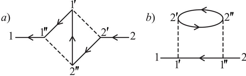
Figure 1:

It is important to emphasize that, in this technique, no Green’s line can link vertices belonging to the same interaction line (item 5). Such elements are known AGD1 ; BKY ; Mattuck to be involved into the diagram technique based on the ideal gas approximation. Those diagrams can include both Green’s lines leaving and entering the same vertex (“bubbles”) and Green’s lines linking the vertices of the same interaction line (“oysters”) Mattuck . The diagrams which contain such elements are impossible in the technique proposed, because, owing to the normal form of the perturbation Hamiltonian, there are no contractions between operators that stand under the sign of the same $N$-product. The absence of such diagrams in this technique is also natural, because the diagrams made up of these elements define the SCF approximation which has already been taken into account in this case in the main approximation. In Fig. 1, as an example, the diagrams of the second order are shown which define the corrections to the one-particle GF in the field representation.

The formulated diagram technique, as well the technique based on the approximation of non-interacting particles AGD1 admits the diagrams to be summed up by separate blocks and the graphic methods of summation to be used.

The diagrams for the temperature scattering matrix are constructed by the same rules, as those for the construction of GFs. The former differ from the latter by the absence of external lines. As is known AGD1 ; BKY , it does not allow the graphic summation of the infinite sequences of diagrams to be carried out in this case.

For the practical use of the diagram technique, it is more convenient to pass to the frequency representation. In this case, the rules of the diagram technique undergo the following modifications:

1) every Green’s line is associated with Fourier-component (57) $G^{(0)}\!(1,2;\omega_{n})$, and every external incoming line should be associated with a frequency with the minus sign;

2) every dashed line is associated with the potential $\underline{\tilde{U}}(1,2)=U({\bf r}_{1},{\bf r}_{2})(\delta_{\alpha_{1}\alpha_{2}}-\delta_{\alpha_{1}\bar{\alpha}_{2}})$;

3) the frequency conservation law must be fulfilled: the sum of the frequencies of Green’s lines which enter the end points of every dashed line of the interaction is equal to the sum of frequencies of the outgoing lines, which is taken into account by introducing the multiplier $\Delta(\omega_{n_{1}}+\omega_{n_{2}}-\omega_{n_{3}}-\omega_{n_{4}})$; with $\Delta(\omega)=1$ if $\omega=0$, and $\Delta(\omega)=0$ otherwise;

4) the additional multiplier $T^{n-L/2}$ emerges before the expression that correspond to the diagram.

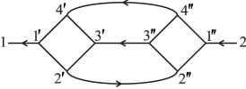
Figure 2:

Now, let us formulate the rules of the diagram technique in the case where the quasiparticle description is used. Taking into account that the adjacent operators can be permutated under the sign of normal product with changing the sign, Hamiltonian (47) can be represented in the form

$$\begin{array}[]{ll}\displaystyle{H_{C}=\frac{1}{4!}\sum_{1234}\tilde{U}_{1234}N(\gamma_{1}\gamma_{2}\gamma_{3}\gamma_{4})\,,}\end{array}$$ (66)

where the antisymmetrized potential

$$\begin{array}[]{ll}\displaystyle{\tilde{U}_{1234}=U_{1234}\!+\!U_{1342}\!+\!U_{1423}\!+\!U_{2314}\!+\!U_{2431}\!+\!U_{3412}-\vspace{3mm}}\\ \displaystyle{\hskip 8.53581pt-U_{1243}\!-\!U_{1324}\!-\!U_{1432}\!-\!U_{2341}\!-\!U_{2413}\!-\!U_{3421}.}\end{array}$$ (67)

was introduced. Let us introduce a notation for the potential

$$\begin{array}[]{ll}\displaystyle{\tilde{U}(1,2,3,4)=\tilde{U}_{1234}\,\delta(\tau_{1}-\tau_{2})\,\delta(\tau_{1}-\tau_{3})\,\delta(\tau_{1}-\tau_{4})\,,}\end{array}$$ (68)

which is antisymmetric with respect to the permutation of variables. A single digit in the potential $\tilde{U}(1,2,3,4)$ designates the following set of variables: $1\!=\!(i_{1},\alpha_{1},\tau_{1})$. Every square in the diagram is confronted with the matrix element of the interaction potential

$$\begin{array}[]{ll}\displaystyle{\tilde{U}(1,2,3,4)\hskip 22.76219pt\textrm{---}\hskip 22.76219pt\scalebox{0.65}[0.65]{\includegraphics[bb=28 482 85 510]{IV.eps}}\quad,\vspace{3mm}}\end{array}$$

while every Green’s line with the zero-order approximation of the GF in the quasiparticle representation. Indices at the square vertices must be arranged either clockwise or counterclockwise in that order as they enter into the expression for the matrix element (68).

Thus, the rules for calculating the contribution of the $n$-th order to the Green’s quasiparticle function are as follows:

1) draw $n$ squares that correspond to the matrix elements of the interaction potential;

2) link the vertices of different squares with solid lines in all such topologically nonequivalents ways, that two vertices of a square serve as sinks for one Green’s line each and two other vertices of the same square be the sources of one Green’s line each;

3) confront the graphic representations with their analytical expressions; sum up over the variables related to each vertex and integrate over “time” variables;

4) put the multiplier $(-1)^{n+k+Q}/P_{n}$ before the expression that has been constructed according to the diagram, where $n$ is the order of the diagram, $k$ the number of closed loops in it, $Q$ the number of permutations which are necessary to arrange the external indices linked by a solid line in that order as they enter into the analytical record of the GF, $P_{n}$ the number of permutations of the indices in the square vertices that do not result in new expressions.

In the quasiparticle representation, we get only one diagram of the second order which is shown in Fig. 2.

For the frequency representation of quasiparticle GFs, the rules are modified in the same way as in the case of field GFs.

8. Similarly as in the quantum-field approach that uses the model of independent particles as the zero-order approximation, the concept of self-energy and vertex parts can be introduced in the approach that is developed here, and the Dyson’s equation that couples those two functions can be derived. The equation for a one-particle GF can be presented in the following form:

$$\begin{array}[]{ll}\displaystyle{\frac{\partial G(1,2)}{\partial\tau_{1}}=-\delta(1-\bar{2})-\vspace{2mm}}\\ \displaystyle{\hskip 8.53581pt-\int\!d3\,\big{[}H(1,\bar{3})+W(1,\bar{3})+\Sigma(1,\bar{3})\big{]}G(3,2)\,,}\end{array}$$ (69)

where the self-energy function $\Sigma(1,2)$ is defined by the relation

$$\begin{array}[]{ll}\displaystyle{\int\!d3\,\Sigma(1,\bar{3})\,G(3,2)=\frac{1}{2}\int\!d3\,\tilde{U}(1,3)\times\vspace{3mm}}\\ \displaystyle{\hskip 5.69054pt\times\big{[}G(1,3,\bar{3},2)\!+\!G^{(0)}\!(\bar{3},3)\,G(1,2)\!-\!2\,G^{(0)}\!(\bar{3},1)\,G(3,2)\big{]}.}\end{array}$$ (70)

Formula (69) includes the functions

$$\begin{array}[]{ll}\displaystyle{H(1,\bar{3})=H_{\alpha_{1}\bar{\alpha}_{3}}(q_{1},q_{3})\,\delta(\tau_{1}-\tau_{3})\,,\vspace{3mm}}\\ \displaystyle{W(1,\bar{3})=W_{\alpha_{1}\bar{\alpha}_{3}}(q_{1},q_{3})\,\delta(\tau_{1}-\tau_{3})\,,}\end{array}$$ (71)

where

$$\begin{array}[]{ll}\displaystyle{H_{\alpha\alpha^{\prime}}(q,q^{\prime})=\left[\begin{array}[]{cc}0&H(q,q^{\prime})\\ -H^{*}(q,q^{\prime})&0\\ \end{array}\right]\,,\vspace{4mm}}\\ W_{\alpha\alpha^{\prime}}(q,q^{\prime})=\left[\begin{array}[]{cc}\Delta(q,q^{\prime})&W(q,q^{\prime})\\ -W^{*}(q,q^{\prime})&-\Delta^{*}(q,q^{\prime})\\ \end{array}\right]\,.\end{array}$$

With regard for the equations for a GF in the SCF approximation, we obtain the known relation for the self-energy function:

$$\begin{array}[]{ll}\displaystyle{G(1,2)=G^{(0)}\!(1,2)+\int\!\!d3d4\,G(1,\bar{3})\,\Sigma(3,\bar{4})\,G^{(0)}\!(4,2)\,.}\end{array}$$ (72)

The vertex part $\Gamma(1,2,3,4)$ is defined by the formula

$$\begin{array}[]{ll}\displaystyle{G(1,2,3,4)=\vspace{3mm}}\\ \displaystyle{\hskip 8.53581pt=G(1,2)\,G(3,4)+G(1,4)\,G(2,3)-G(1,3)\,G(2,4)+\vspace{3mm}}\\ \displaystyle{\hskip 5.69054pt+\int\!\!d1^{\prime}d2^{\prime}d3^{\prime}d4^{\prime}\,\Gamma(1^{\prime},2^{\prime},3^{\prime},4^{\prime})\times\vspace{3mm}}\\ \displaystyle{\hskip 5.69054pt\times\,G(\bar{1}^{\prime},1)\,G(\bar{2}^{\prime},2)\,G(\bar{3}^{\prime},3)\,G(\bar{4}^{\prime},4)\,.}\end{array}$$ (73)

From Eq. (70), taking Eq. (73) into account, we obtain the Dyson’s equation which establishes a relation between the self-energy and vertex parts in Fermi systems with spontaneously broken symmetry:

$$\begin{array}[]{ll}\displaystyle{\Sigma(1,2)\!=\!\frac{1}{2}\int\!d3\,\tilde{U}(1,3)\Big{\{}\!\big{[}G(3,\bar{3})-G^{(0)}\!(3,\bar{3})\big{]}\delta(1-\bar{2})-\vspace{3mm}}\\ \displaystyle{\hskip 8.53581pt-2\big{[}G(3,1)-G^{(0)}\!(3,1)\big{]}\delta(2-3)\Big{\}}+\vspace{3mm}}\\ \displaystyle{\hskip 8.53581pt+\frac{1}{2}\int\!d1^{\prime}d2^{\prime}d3^{\prime}d3\,\tilde{U}(1,3)\times\vspace{3mm}}\\ \displaystyle{\hskip 8.53581pt\times\Gamma(1^{\prime},2^{\prime},3^{\prime},2)\,G(\bar{1}^{\prime},1)\,G(\bar{2}^{\prime},3)\,G(\bar{3}^{\prime},3)\,.}\end{array}$$ (74)

The poles of the vertex function introduced by relation (73) define the dispersion law of collective excitations in the many-body system.

The methods of quantum field theory applied in statistical physics were extended in this work to describe any eligible states in non-relativistic Fermi systems with spontaneously broken symmetry. We managed to do this, mainly, owing to two circumstances. First, it is the SCF model formulated in the most general form that was used as the main approximation. Secondly, it is the procedure for calculating the quasiaverages which uses the fields that are defined by this model. It is essential that, in the given approach, the correlation Hamiltonian considered as a perturbation can be presented in the normal form, which allows a plenty of diagrams not contributing to the final result to be excluded from consideration and the diagram technique to be presented in a compact form. The approach suggested does not contain any assumptions and is based only on the general principles of quantum mechanics and statistical physics. It can be applied for regular researches of equilibrium properties of many-particle systems with spontaneously broken symmetry (magnetically and spatially ordered, superconducting, superfluid, etc. systems) and the phenomena in them at a microscopic level. The method proposed can be extended onto the description of non-relativistic Bose systems with spontaneously broken symmetry, in particular, of superfluid systems with broken phase symmetry Poluektov5 ; Poluektov6 . In author’s opinion, the general approach developed in this work can also be effectively used for a proper description of states with spontaneously broken symmetry in the relativistic field theory and the theory of elementary particles NL ; Goldstone .