Abstract

Gene transcription mediated by RNA polymerase II (pol-II) is a key step in gene expression. The dynamics of pol-II moving along the transcribed region influence the rate and timing of gene expression. In this work we present a probabilistic model of transcription dynamics which is fitted to pol-II occupancy time course data measured using ChIP-Seq. The model can be used to estimate transcription speed and to infer the temporal pol-II activity profile at the gene promoter. Model parameters are estimated using either maximum likelihood estimation or via Bayesian inference using Markov chain Monte Carlo sampling. The Bayesian approach provides confidence intervals for parameter estimates and allows the use of priors that capture domain knowledge, e.g. the expected range of transcription speeds, based on previous experiments. The model describes the movement of pol-II down the gene body and can be used to identify the time of induction for transcriptionally engaged genes. By clustering the inferred promoter activity time profiles, we are able to determine which genes respond quickly to stimuli and group genes that share activity profiles and may therefore be co-regulated. We apply our methodology to biological data obtained using ChIP-seq to measure pol-II occupancy genome-wide when MCF-7 human breast cancer cells are treated with estradiol (E2). The transcription speeds we obtain agree with those obtained previously for smaller numbers of genes with the advantage that our approach can be applied genome-wide. We validate the biological significance of the pol-II promoter activity clusters by investigating cluster-specific transcription factor binding patterns and determining canonical pathway enrichment. We find that rapidly induced genes are enriched for both estrogen receptor alpha (ER$\alpha$) and FOXA1 binding in their proximal promoter regions.

Author Summary

Cells express proteins in response to changes in their environment so as to maintain normal function. An initial step in the expression of proteins is transcription which is mediated by RNA polymerase II (pol-II). To understand changes in transcription arising due to stimuli it is useful to model the dynamics of transcription. We present a probabilistic model of pol-II transcription dynamics that can be used to compute RNA transcription speed and infer the temporal pol-II activity at the gene promoter. The inferred promoter activity profile is used to determine genes that are responding in a coordinated manner to stimuli and are therefore potentially co-regulated. Model parameters are inferred using data from high-throughput sequencing assays, such as ChIP-Seq and GRO-Seq, and can therefore be applied genome-wide in an unbiased manner. We apply the method to pol-II ChIP-Seq time course data from breast cancer cells stimulated by estradiol in order to uncover the dynamics of early response genes in this system.

Introduction

Transcription mediated by RNA polymerase II (pol-II) is an essential process in the expression of protein-coding genes in eukaryotes. Transcription is dependent upon a number of sequential and dynamic events, such as recruitment of pol-II to the transcriptional start site, activation of pol-II through phosphorylation of its C-terminal domain, elongation of the nascent transcript through the transcribed region and termination [1]. Each of these steps may be rate-limiting and can therefore affect the level of gene expression. In this manuscript, we describe a simple probabilistic model of transcription whose parameters can be inferred using time-series data such as pol-II ChIP-Seq data [2] or nascent transcript measurement by GRO-Seq that reports markers of transcriptional activity [3]. This model can be used to identify transcriptionally engaged genes, estimate their transcription rates and infer transcriptional activity adjacent to the promoter. The transcriptional dynamics of estrogen responsive genes in a breast cancer cell line were described by fitting this model to pol-II ChIP-seq time course datasets.

Chromatin immunoprecipitation, in conjunction with massively parallel sequencing (ChIP-seq) evaluates interactions between proteins and DNA, and, for example, can be used to monitor the presence of pol-II on DNA. Estimating the amount of pol-II associated with a transcribed gene provides a measure of transcriptional activity [2]. Sequential measurement of pol-II occupancy on genes released from transcriptional blockade, for example, in response to stimuli, reveal a wave of transcription moving through the body of the responding transcript.

A number of studies have attempted to determine the rate of transcription through modelling the dynamics of pol-II. Darzacq et al. fit a mechanistic model of pol-II transcription to nascent RNA data at a single locus and obtained a transcription speed of 4.3 kilobases per minute [4]. Wada et al. activated transcription of genes greater than 100 kbp in length and estimated the transcription speeds using a model that measures an intronic RNA signal through taking advantage of co-transcriptional splicing. They obtain an average transcription rate of 3.1 kbp min^-1 [5]. Singh and Padget (2009) reversibly inhibit transcription to determine the transcription rate of 9 genes, all of which were greater than 100 kbp which had an average transcription rate of 3.79 kbp min^-1 [6]. The data used in these studies have good temporal resolution (e.g. samples every 7.5 min in [5]) and reliably allow fitting of mathematical models or the direct measurement of transcription speed, however, only for a limited set of long genes. In contrast, high throughput data sets such as ChIP-Seq, can be used to uncover transcription dynamics genome-wide but typically have much lower temporal resolution, motivating the development of alternative modelling approaches that report genome-wide transcription rates.

One way around the low temporal resolution of typical high-throughput time course data is to employ a non-parametric model of the biological signals of interest. In many cases we expect these signals to vary continuously and smoothly in time, when averaged over a cell population, and a Gaussian process model provides a convenient non-parametric model in such cases [7]. Gaussian processes have recently found applications in a range of biological system models  [8, 9, 10, 11].

Here we present a Gaussian process model of transcription dynamics which can be fitted to genome-wide pol-II occupancy data measured using ChIP-Seq. The model describes the movement of pol-II through the gene body and combines a flexible model of promoter-proximal pol-II activity with a reliable estimate of transcription speed. By identifying genes which fit the model well, we provide a useful method to identify actively transcribed genes. The model does not assume a constant transcription speed and can therefore identify variable rates of transcription, for example due to transcriptional pausing. Model parameters are inferred using either maximum likelihood (ML) estimation or via Bayesian inference using Markov chain Monte Carlo (MCMC) sampling. The Bayesian approach provides confidence intervals for parameter estimates and can incoporate priors that capture domain knowledge, e.g. the expected range of transcription speeds, based on previous experiments.

We fit our model to a pol-II ChIP-Seq time course dataset from MCF7 breast cancer cells stimulated with estradiol. The model is used to identify the set of transcriptionally engaged genes and estimate their mean transcription rate and transcriptional activity near the promoter. By clustering promoter activity profiles, potential co-regulated groups of genes are identified, particularly those that respond rapidly to estrogen signalling. Subsequent characterisation of transcription factor (TF) binding sites in proximity to the promoters of genes within clusters provides a means of classifying groups of promoters that are responsive to the binding of specific combinations of TF’s. Additionally, publically available ChIP-Seq datasets of TF profiles from the same system were used to identify cluster-specific patterns in TF-binding. The rates of transcription estimated by our model are consistent with the literature [4, 5] but with the advantage that our method allows the computation of transcription speeds genome-wide.

Our methodology has a number of advantages. We do not require data with high temporal resolution, making it feasible to model transcriptional dynamics genome-wide using ChIP-Seq or GRO-Seq time course data. We infer transcription rates for all genes in an unbiased manner and by using Bayesian parameter estimation we are able to associate our transcription rate estimates with confidence intervals. Our model is non-parametric and therefore does not make very strong assumptions about the temporal changes in transcriptional activity. Fitting the model genome-wide allows us to identify and filter out transcripts where pol-II does not travel down the gene body. This provides a principled method to identify responsive genes, in particular, early acting estrogen responsive genes in the specific application considered here. Since our model does not enforce a uniform transcription speed over the entire gene body, we can take into account phenomena such as pol-II pausing which would result in a non-uniform transcription speed. We also use this model to infer the promoter activity of transcriptionally engaged genes, to identify co-regulated gene modules downstream of estrogen signalling.

Methods

Visualizing pol-II ChIP-seq reads mapped to transcriptional units at multiple time points following the addition of estradiol to MCF7 cells reveals the motion of pol-II through the gene body of estrogen responsive genes (see Figure 1). Computing the average pol-II occupancy over successive gene segments describes the motion of the transcription wave. Thereafter, fitting a model capable of smoothly interpolating between observed time points and by determining the time taken for pol-II to move from one gene segment to the next determines if pol-II is transcriptionally engaged on a given transcript and the speed at which it is moving through this transcriptional unit. We use a convolved Gaussian process to model the relationship between the pol-II signal at different regions of the gene and across time. Model parameters are determined using maximum likelihood (ML) or Bayesian inference via Markov chain Monte Carlo (MCMC) to determine genes of interest and moreover, in the case of MCMC, determine confidence intervals for our parameter estimates.

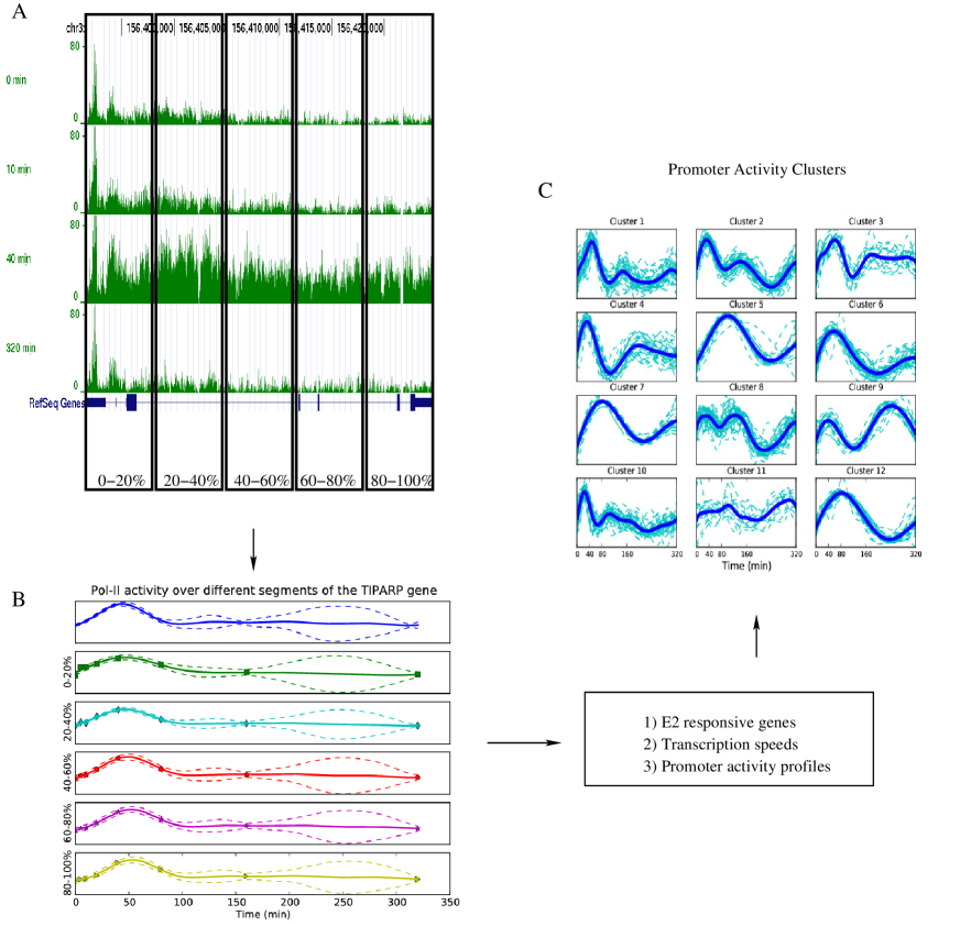
Figure 1: Pol-II ChIP-seq data for the TIPARP gene shows a transcription wave moving down the gene. The transcription dynamics model captures this motion and allows us to estimate transcription speeds. In this case the gene is divided into 5 segments and we estimate the speed to be approxiamtely 2 kilobases per minute. Figure A shows the raw ChIP-seq reads at different times between 0 and 320 min. The top panel of Figure B shows the inferred promoter activity profile. The next five panels show the inferred profiles for the five gene segments corresponding to $0-20\%,\ldots,80\%-100\%$ of the gene. By clustering these promoter activity profiles as shown in Figure C, we are able to group genes into clusters that are likely to be co-regulated and in particular we identify the clusters that respond most rapidly to estrogen signalling.

Convolved Gaussian Process Model

A Gaussian process (GP) is a distribution over the space of functions. This distribution is completely specified by a mean function $m(t)$ and a covariance function $k(t,t^{\prime})$. A function $f(t)$ is said to be drawn from a Gaussian process $\mathcal{GP}(m(t),k(t,t^{\prime}))$ if $f(t)$ at any finite collection of points has a multivariate Gaussian distribution with mean vector and covariance matrix specified by $m(t)$ and $k(t,t^{\prime})$, respectively. GPs provide a powerful framework for non-parametric regression [7]. If a function is assumed to be drawn from a GP with known mean and covariance function, we can infer the function value and associated uncertainty at unobserved locations given noise-corrupted observations. GPs have recently been applied in modelling biological systems, e.g. modelling protein concentrations as latent variables in differential equation models of transcriptional regulation [8, 9] and modelling spatial gene expression [11].

Here we introduce a novel application of GPs to modelling the spatio-temporal dynamics of pol-II occupancy during transcription. Convolved GPs allow the modelling of correlations between multiple coupled data sources. In our case these data sources are the pol-II occupancy over time collected at different locations along the transcribed region of a gene. Modelling the data as a convolved process borrows information from these different data sources in estimating the model parameters and inferring the underlying signal in the data. Also, we find that convolved GPs are necessary to account for changes in the shapes of signals observed at different regions of the gene. In linear systems theory, the output $y(t)$ of a linear time-invariant system whose impulse response is $h(t)$ is given by the convolution of the input $x(t)$ and $h(t)$, that is $y(t)=\int_{-\infty}^{\infty}h(\tau)x(t-\tau)d\tau$. If different sets of observations are believed to be related, they can be modeled as the outputs of different linear systems in response to a single input. If this input is modeled as a GP, then it will form a joint GP together with all the outputs and data from one output stream will be useful in inferring the rest [12, 13, 14, 15, 16, 17, 18, 19, 20]. In our case, incorporating the data from multiple spatially separated regions of the genes allows us to infer an underlying function that links all these regions. This proves useful as a summary of the transcription dynamics of the gene and we show that it provides useful insights into potential coregulation.

Model Description

In order to capture the movement of the transcription wave through transcriptional units, we divide each gene into $I$ segments and compute time series of pol-II occupancy for each of the segments. Due to the low temporal resolution characteristic of high-throughput datasets, the time series between measurements must be inferred. To this end, we model the pol-II occupancy $y_{i}(t)$ in each segment $i\in\{1,\ldots,I\}$ as the convolution of a latent process $f(t)$ which is shared by all segments and a (possibly delayed) smoothing kernel $k_{i}(\tau-D_{i})$ corrupted by an independent white Gaussian noise process $\epsilon_{i}(t)$ with zero mean and variance $\sigma_{i}^{2}$ [15, 16]. That is

$$y_{i}(t)=\alpha_{i}\int_{-\infty}^{\infty}f(t-\tau)k_{i}(\tau-D_{i})d\tau+\epsilon_{i}(t),$$ (1)

where $\alpha_{i}$ is a scale factor and $D_{i}$ is the delay of each segment. The latent process $f(t)$ is modeled as a random function drawn from a GP with zero mean and a squared exponential covariance function (defined in Equation (4) below). The smoothing kernel is assumed to be Gaussian, that is

$$k_{i}(\tau)=\frac{1}{\sqrt{2\pi}\ell_{i}}\exp\Bigg{(}-\frac{\tau^{2}}{2\ell_{i}^{2}}\Bigg{)}.$$ (2)

The estimated delay $D_{i}$ of each smoothing kernel models the amount of time it takes the ‘transcription wave’ to reach the corresponding gene segment. This is used to estimate the transcription speed. Biologically the latent function can be thought of as modeling activity at the promoter while the smoothing kernel accounts for ‘diffusion’ of the transcription wave. This diffusion phenomenon is observed when time series of pol-II occupancy over different sections of a gene are plotted, with the transcription wave seen to spread out (see Figure 4). This phenomenon may be due to an initially synchronized cell population becoming less synchronized over time, resulting in broadening of the pol-II occupancy distribution over time. The parameter $\ell_{i}$ captures the amount of ‘spread’ observed at the $i$th segment. It also serves as a measure of the loss of synchrony between the cells of the population when the transcription wave is observed at the $i$th segment.

Using equation (1), we can compute the covariance between the pol-II occupancy at various segments of the gene. We have

$$\mathsf{cov}[y_{i}(t),y_{j}(t^{\prime})]=\alpha_{i}\alpha_{j}\int_{-\infty}^{\infty}\int_{-\infty}^{\infty}k_{f}(t-\tau,t^{\prime}-\tau^{\prime})k_{i}(\tau-D_{i})k_{j}(\tau^{\prime}-D_{j})d\tau d\tau^{\prime}+\sigma_{i}^{2}\delta_{ij}\delta_{tt^{\prime}}$$ (3)

where

$$k_{f}(t,t^{\prime})=\sigma_{f}^{2}\exp\Bigg{(}-\frac{(t-t^{\prime})^{2}}{2\ell_{f}^{2}}\Bigg{)}.$$ (4)

Equation (3) can be evaluated in closed form using the fact that the product of two Gaussians yields an un-normalized Gaussian [7]. Exploiting this fact we get

$$\mathsf{cov}[y_{i}(t),y_{j}(t^{\prime})]=\alpha_{i}\alpha_{j}\frac{\sigma_{f}^{2}\ell_{f}}{\sqrt{\ell_{f}^{2}+\ell_{i}^{2}+\ell_{j}^{2}}}\exp\Bigg{(}-\frac{(t^{\prime}-t+D_{i}-D_{j})^{2}}{2(\ell_{f}^{2}+\ell_{i}^{2}+\ell_{j}^{2})}\Bigg{)}+\sigma_{i}^{2}\delta_{ij}\delta_{tt^{\prime}}.$$ (5)

Similarly,

$$\mathsf{cov}[f(t),y_{i}(t^{\prime})]=\alpha_{i}\frac{\sigma_{f}^{2}\ell_{f}}{\sqrt{\ell_{f}^{2}+\ell_{i}^{2}}}\exp\Bigg{(}-\frac{(t^{\prime}-t-D_{i})^{2}}{2(\ell_{f}^{2}+\ell_{i}^{2})}\Bigg{)}.$$ (6)

Parameter Estimation and Inference

Let $\mathbf{y}_{i}=[y_{i1},\ldots,y_{iN}]^{\top}$ be a vector of observations of pol-II occupancy over the i$th$ gene segment and let $\mathbf{Y}=[\mathbf{y}_{1}^{\top},\ldots,\mathbf{y}_{I}^{\top}]^{\top}$ be a vector formed by concatenating all the observations for a single gene. $N$ is the number of observation time points and $I$ is the number of gene segments so for a single gene $\mathbf{Y}$ is a vector of length $NI$. We have

$$p(\mathbf{f},\mathbf{Y}|\Theta)=\mathcal{N}([\mathbf{f},\mathbf{Y}];\mathbf{0},\mathbf{K}),$$ (7)

where

$$\mathbf{K}=\left[\begin{array}[]{cccc}\mathbf{K}_{\mathbf{f,f}}&\mathbf{K}_{\mathbf{f,y_{1}}}&\ldots&\mathbf{K}_{\mathbf{f,y_{I}}}\\ \mathbf{K}_{\mathbf{y_{1},f}}&\mathbf{K}_{\mathbf{y_{1},y_{1}}}&\ldots&\mathbf{K}_{\mathbf{y_{1},y_{I}}}\\ \vdots&\vdots&\ddots&\vdots\\ \mathbf{K}_{\mathbf{y_{I},f}}&\ldots&\ldots&\mathbf{K}_{\mathbf{y_{I},y_{I}}}\end{array}\right]$$ (8)

and $\Theta=\{\sigma_{f},\ell_{f},\{\alpha_{i},D_{i},\ell_{i},\sigma_{i}\}_{i=1}^{I}\}$ are the parameters of our model which will be fitted on a gene by gene basis. The elements of $\mathbf{K}$ are computed using equations (4), (5), and (6). By marginalizing over the latent function $\mathbf{f}$, we obtain the marginal likelihood $p(\mathbf{Y}|\Theta)$. Maximum likelihood estimates of the parameters $\Theta$ are readily obtained by maximizing the log marginal likelihood using gradient-based optimisation.

For a fully Bayesian approach, we take advantage of the fact that the parameters are positive and bounded. We transform the parameters using a logit transform and work with unconstrained variables. We place a Gaussian prior over the parameters in the transformed domain and draw samples from the posterior using the Hamiltonian Monte Carlo (HMC) algorithm [21] (A more detailed description of the priors is included in the supplementary material).

Code to implement the method is freely available as a Python package, PyPol-II, which can be downloaded from https://github.com/ciiram/PyPol_II.

Estimation of Average Transcription Speed

When fitting the model, we fix $D_{1}=0$ to ensure identifiability. The average transcription speed is computed by assuming that the value of $D_{i}$ is an indicator of how long it takes the ‘transcription wave’ to reach the corresponding gene segment. That is, $D_{2}$ is the amount of time it takes to transcribe 20% of the gene, $D_{3}$ 40% etc. To obtain confidence intervals on the delay estimates, MCMC was performed to get samples of the parameters.

To compute the average transcription speed we plot the position along the gene in base pairs (bp) versus the delay in minutes and compute a linear regression through the origin. The slope of the regression line gives us the transcriptional speed. Each sample of the parameters provides a set of delay estimates from which we obtain a speed estimate.

Alternative Methods for Time Delay Inference

A key component of our method involves the estimation of delay between time series observed at different segments of the gene. The study of time delay between related time series has received attention from a number of researchers for a long time [22]. The application areas range from signal processing to astronomy [23]. The classic approach to time delay estimation involves computing the cross-correlation between the related time series and determining the value of delay for which this function is maximised. Consider two signals $y_{1}(t)$ and $y_{2}(t)$ given by

$$y_{1}(t) = f(t)+n_{1}(t)$$

$$y_{2}(t) = f(t-D)+n_{2}(t)$$ (9)

where $n_{1}(t)$ and $n_{2}(t)$ are uncorrelated noise processes. The cross-correlation function is given by $R_{y_{1},y_{2}}(\tau)=\mathbf{E}[y_{1}(t)y_{2}(t-\tau)]$ where $\mathbf{E}$ denotes the expectation operator. The value of $\tau$ that maximises $R_{y_{1},y_{2}}(\tau)$ yields an estimate of the delay $D$. When the signals are sampled at $N$ equally spaced time points $t_{0},\ldots,t_{N-1}$ with spacing $T$ between samples, the discrete time equivalent of $R_{y_{1},y_{2}}(\tau)$ is readily estimated. Let $y_{1}[n]=y_{1}(nT)$, the discrete cross-correlation is estimated as

$$\hat{R}_{y_{1},y_{2}}(kT)=\frac{1}{N}\sum_{n=0}^{N-1-k}y_{1}[n]y_{2}[n+k].$$

The delay is estimated by finding the value of $k$ for which $\hat{R}_{y_{1},y_{2}}(kT)$ is maximised. The corresponding delay estimate is $kT$. However, this approach doesn’t work well when the time series are unevenly sampled as is the case in several astronomical and biological studies. A number of techniques have been developed to handle unevenly sampled time series including the discrete correlation function (DCF) [24], and the more recent kernel based approaches [25, 26]. The DCF is computed as follows, for all $i,j\in\{0,\ldots,N-1\}$ the time differences $\Delta_{ij}=|t_{i}-t_{j}|$ are binned into discrete bins of size $\Delta\tau$. The DCF at $\tau$ is given by [24, 25]

$$DCF(\tau)=\frac{1}{|S(\tau)|}\sum_{(i,j)\in S(\tau)}\frac{(y_{1}[i]-\bar{y_{1}})(y_{2}[j]-\bar{y_{2}})}{\sqrt{(\sigma_{y_{1}}^{2}-\sigma_{y_{1i}}^{2})(\sigma_{y_{2}}^{2}-\sigma_{y_{2j}}^{2})}},$$ (10)

where

$$S(\tau)=\{(i,j)|\Delta_{ij}\in[\tau-\Delta\tau,\tau+\Delta\tau]\},$$ (11)

and $\sigma_{y_{1}}^{2}$ and $\sigma_{y_{2}}^{2}$ are the variances of the observation streams while $\sigma_{y_{1i}}^{2}$ and $\sigma_{y_{2j}}^{2}$ are observation error variances.

In the kernel based approach of [25], the underlying function $f(t)$ of equation (Alternative Methods for Time Delay Inference) is modelled as the sum of a fixed number of kernels centered at the observation times. That is

$$f(t)=\sum_{i=0}^{N-1}\alpha_{i}K(c_{i},t)$$ (12)

where

$$K(c_{i},t)=\exp\Bigg{(}-\frac{(t-c_{i})^{2}}{\sigma_{i}^{2}}\Bigg{)}.$$ (13)

The value of $D$ that minimises the estimation error is the delay estimate. Our implementation follows that presented in [25] where we assumed a fixed kernel width. This kernel width is determined by leave one out cross-validation.

Benchmark Data

We used synthetic data and previously published experimental data to assess our novel method’s performance. To generate the synthetic data, the underlying function $f(t)$ of equation (Alternative Methods for Time Delay Inference) was given as a sum of Gaussian kernels. That is

$$f(t)=\sum_{i=1}^{N}\beta_{i}\exp\Bigg{(}-\frac{(t-c_{i})^{2}}{\sigma_{i}^{2}}\Bigg{)}.$$

N was fixed at 20 and the observation interval $t\in[0,10]$. $\beta_{i}$, $\sigma_{i}$ and $c_{i}$ were generated at random with $\beta_{i}\in[0,1]$, $\sigma_{i}\in(0.5,1.5]$ and $c_{i}\in[2.5,5]$. A random delay $D\in[1,2.5]$ was used to generate the observations which were corrupted by additive Gaussian noise with $\sigma_{n}=0.001$. To determine the effect of number of observations on the quality of inference we compute the Median Normalised Square Error (MNSE) of the estimated delay $\frac{\|D-\hat{D}\|_{2}^{2}}{\|D\|_{2}^{2}}$ as a function of the number of observations for 50 random realisations of the the signals. We also investigated the effect of distorting the shape of the observed signals by introducing convolution. In real signals the restriction that the shape remains unchanged sometimes leads to poor results. The parameters of the smoothing kernel in equation (1) were generated at random with $\alpha_{i}\in[0,1]$ and $\ell_{i}\in(0.625,2.5]$.

To assess performance of our method on a well characterised real-world dataset we obtained a dataset from Singh and Padgett [6] where the delay in appearance of pre-mRNA signal at exon-intron junctions was used to compute estimates of transcription speed for 9 genes. To generate the data, transcription was reversibly inhibited in vivo using 5,6-dichlorobenzimidazole 1-beta-D-ribofuranoside (DRB) and the pre-mRNA measured after the inhibitor was removed. As verified by the authors, the kinetics of pol-II and pre-mRNA are similar hence we expect good performance on this dataset to indicate applicability of our method to pol-II ChIP-seq data.

pol-II ChIP-Seq Data

To demonstrate an application to pol-II ChIP-Seq data, we apply our model to investigate the transcriptional response to Estrogen Receptor signalling. ChIP-seq was used to measure pol-II occupancy genome-wide when MCF-7 breast cancer cells are treated with estradiol (E2). Cells were put in estradiol free media for three days. This is defined media devoid of phenol red (which is estrogenic) containing 2% charcoal stripped foetal calf serum. The charcoal absorbs estradiol but not other essential serum components, such as growth factors. This results in basal levels of transcription from E2 dependent genes. The cells are then incubated with E2 containing media, which results in the stimulation of estrogen responsive genes. The measurements were taken at logarithmically spaced time points 0, 5, 10, 20, …, 320 minutes after E2 stimulation.

Raw reads were mapped onto the human genome reference sequence (NCBI_build37) using the Genomatix Mining Station (software version 3.2.1). The mapping software on the Mining Station is an index based mapper that uses a shortest unique subword index generated from the reference sequence to identify possible read positions. A subsequent alignment step is then used to get the highest-scoring match(es) according to the parameters used. We used a minimum alignment quality threshold of 92% for mapping and trimmed 2 basepairs from the ends of the reads to account for deterioration in read quality at the 3’ end. The software generates separate output files for uniquely mapped reads and reads that have multiple matches with equal score. We only used the uniquely mapped reads. On average about 66% of all reads could be mapped uniquely. The data are available from the NCBI Gene Expression Omnibus under accession number GSE44800.

Time series of pol-II occupancy over various segments of genes were computed in reads per million (RPM) [27] using BEDtools [28, 29]. The genes were divided into 200bp bins and the RPM computed for each bin. The occupancy in a particular gene segment was the mean RPM of the bins in that segment. Here, the gene is divided into five segments each representing 20% of the gene.

Results

Assessment on Benchmark Data

We first applied our methodology to synthetic data in order to compare its performance to other methods. We investigated the performance of five methods, namely cross-correlation (Corr), DCF, the kernel approach of [25] (Kern), a GP approach with no convolution (GP-NoConv), and the convolved GP approach developed in this paper (GP-Conv). Tables 1 and 2 show the MNSE for the different delay estimation methods as a function of the number of observations for synthetic data without convolution and with convolution respectively. Note that the kernel and DCF methods require an estimate of the noise variance and in this simulation study we provide the algorithms with the true value, but that would not be known in practice. We see that when no convolution is introduced, the kernel method performs well but is outperfomed by both GP methods. When convolution is introduced the kernel method appears to break down and as expected the GP-Conv outperforms the other techniques.

We next applied the model to pre-mRNA data from Singh and Padgett [6] where the delay in appearance of pre-mRNA signal at exon-intron junctions was used to compute estimates of transcription speed for 9 genes. Figure 2 shows the pre-mRNA signal for the SLC9A9 gene (the same data shown in Figure 4d of [6]). The delays read from these plots were used in [6] to determine transcription speeds. Figure 3 shows the fit obtained using the kernel method, GP-NoConv and GP-Conv respectively. Table 3 shows the delays read off the plots as well as values obtained using the five delay estimation algorithms for different regions of the nine genes presented in [6]. In each row the delay estimate with the lowest normalised square error is highlighted. Table 4 shows the MNSE for the five delay estimation algorithms for all the genes. We see that the convolved GP method developed in this paper outperforms the other techniques. This method has the added advantage of inferring a latent function which links all the observations and which can be used for downstream analysis. Also, when analysis is genome-wide, reading delays off individual plots is not feasible and furthermore when the sampling intervals are irregularly spaced assigning delays manually would be error prone. These results serve to justify the use of the convolved GP method introduced in this paper.

Number of	MNSE
Observations	Corr	DCF	Kern [25]	GP-NoConv	GP-Conv
6	36e-3	30e-3	4e-3	1.6e-3	2.2e-3
8	44e-3	48e-3	1.0e-3	0.16e-3	0.17e-3
10	11e-3	13e-3	1.2e-3	0.0076e-3	0.012e-3
12	19e-3	18e-3	1.2e-3	0.0018e-3	0.0014e-3

Table 1: MNSE as a function of the number of observations with no convolution.

Number of	MNSE
Observations	Corr	DCF	Kern [25]	GP-NoConv	GP-Conv
6	32e-3	37e-3	17000e-3	0.16e-3	0.053e-3
8	57e-3	61e-3	16000e-3	0.098e-3	0.0057e-3
10	11e-3	15e-3	17000e-3	0.018e-3	0.0021e-3
12	22e-3	31e-3	23000e-3	0.028e-3	0.011e-3

Table 2: MNSE as a function of the number of observations with convolution.

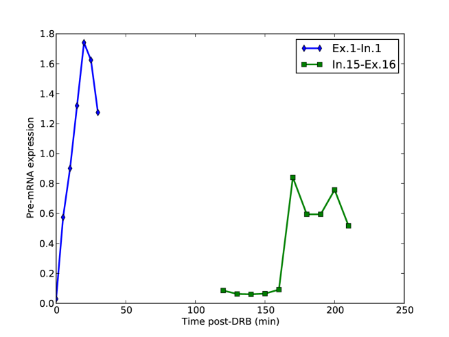
Figure 2: Pre-mRNA espression at exon-intron junctions for the SLC9A9 gene.

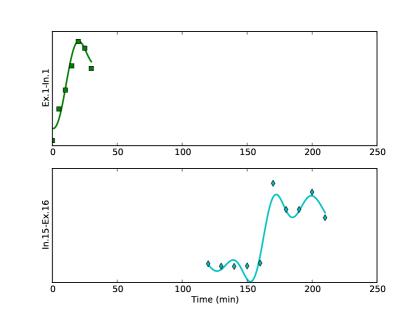
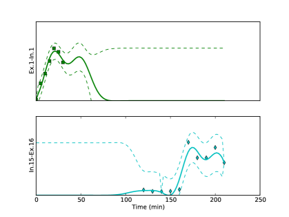
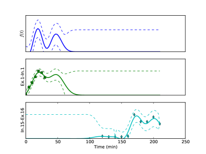
Figure 3: Fits for the SLC9A9 gene using the kernel method (a) and the two GP methods: GP_NoConv (b) and GP_Conv (c). In the GP case we show the 95% confidence interval using dashed lines. In regions with no observations, the uncertainty is large.

Gene	Region	Length	Delay	Corr	DCF	Kern	GP	GP
		(kb)	(min)[6]			[25]	NoConv	Conv
Utrophin	Ex1-Ex2	111	30	15.0	10.8	3.1	46.9	17.4
Utrophin	Ex2-Ex50	174	40	-	49.2	125.5	49.5	46.8
Utrophin	Ex50-Ex51	101	25	-	10.8	67.3	34.1	13.8
Utrophin	Ex51-Ex74	173	40	-	238.3	214.3	9.9	68.5
Utrophin	Ex1-Ex74	561	140	-	135.6	128.6	140.3	146.4
ITPR1	Ex1-Ex5	133	40	45.0	45.5	41.3	49.2	43.2
ITPR1	Ex5-Ex40	105	25	25.0	24.8	23.0	17.4	24.0
ITPR1	Ex1-Ex40	238	65	70.0	69.8	96.4	66.6	67.2
EFNA5	Ex1-Ex2	243	70	65.0	65.4	146.9	69.8	69.9
BCL2	Ex2-Ex3	189	50	5.0	54.9	81.3	65.0	55.0
OPA1	Ex1-Ex29	104	25	20.0	25.0	14.9	27.0	26.8
IFT80	Ex1-Ex20	142	35	40	74.6	35.2	41.6	41.6
CTNNBL1	Ex1-Ex16	178	45	45.0	45.4	39.1	47.2	47.1
KIFAP3	Ex1-Ex20	153	45	45.0	45.4	39.1	46.7	46.7
SLC9A9	Ex1-Ex16	583	160	-	150.2	152.0	153.6	153.5

Table 3: Transcription time estimates for different delay estimation algorithms using the pre-mRNA data from [6]. When sampling times are uneven, cross-correlation results are omitted. In each row the delay estimate with the lowest normalised square error is highlighted.

	Corr	DCF	Kern [25]	GP-NoConv	GP-Conv
MNSE	0.115	1.787	1.974	0.090	0.065

Table 4: MNSE for the 5 delay estimation algorithms for all the genes using pre-mRNA data.

Application to Estrogen Response ChIP-Seq Data

We applied our method to a ChIP-Seq time-course dataset measuring pol-II occupancy genome-wide when MCF-7 cells are treated with estradiol (E2). For our initial experiment, we considered 3,064 genes which exhibit significant increase of pol-II occupancy between 0 and 40 minutes after E2 treatment. These genes were determined by counting the number of pol-II tags on the annotated genes in the RefSeq hg19 assembly at 0 and 40 minutes after E2 treatment and computing the $\mathrm{log}_{2}$ ratio of these counts. We keep those genes where this quantity is greater than one standard deviation above the mean. For these 3,064 genes, we filtered out genes less than 1000bp in length and computed model fits using the ChIP-seq time series data for the remaining 2623 genes. The estimation of the parameters $\{\sigma_{f},\ell_{f},\{\alpha_{i},D_{i},\ell_{i},\sigma_{i}\}_{i=1}^{5}\}$ for a given gene was performed using maximum likelihood with $D_{1}$ fixed at zero, $\sigma_{f}=1$ and the values $\sigma_{i}$ constrained to be equal. Intuitively, one would expect the values of delay $\{D_{i}\}_{i=1}^{5}$ to be non-decreasing. We therefore keep only those genes where this natural ordering is preserved for further analysis. We also discard genes with $\hat{\ell}_{f}\leq 10$ and $\hat{\ell}_{f}\geq 200$ since these are generally seen to be poor fits. Small values of $\hat{\ell}_{f}$ arise when the data is best modelled as a noise process while large values model constant profiles which are not interesting in our analysis. This left us with 383 genes which we consider a conservative set of genes where there is evidence of engaged transcription and where the model parameters can be confidently estimated. To rank these genes we compared the log marginal likelihood of the model fit to that obtained if we assume independence between the segments, which is equivalent to setting the off-diagonal blocks in equation (8) to the zero matrix.

Figure 4 shows the inferred pol-II time profile and histogram of the samples of the delay parameters for three of the top 10 genes found to fit the model well. We note that a relatively small number of activated genes fit the model well. This is primarily because for shorter genes the pol-II occupancy quickly rises over the whole gene such that the temporal resolution of the data cannot capture the wave as it traverses the gene body. With a closer or more evenly spaced time course we would expect a good fit for a greater proportion of activated genes.

Figure 5 shows the linear regression plots using the delay samples for the TIPARP gene. Figure 5 shows the histogram of speed samples from which we can compute the confidence interval for the speed estimate. The 95% confidence interval is indicated in Figure 5 by the red triangle markers (cf. Table 5). Table 5 shows the average transcription speeds for the top 10 genes computed using the samples of the delay parameters. Figure 6 shows a box plot of the average transcription speeds computed using the samples of the delay parameters for these genes.

The advantage of fitting each of the delay parameters independently instead of enforcing a linear relationship is that it allows us to take into account phenomena such as pol-II pausing and provides a means to filter genes where the values of estimated delay are not naturally ordered. Visual inspection of the inferred time series of the top ranked genes is consistent with a ‘transcription wave’ traversing the gene. The transcription wave is especially evident in the longer genes MYH9 and RAB10. This motivates a closer look at long genes. Table 6 shows the average transcription speeds computed using the samples of the delay parameters for the 23 long genes found to fit the pol-II dynamics model well. Grouping these genes according to the magnitude of the median transcription speed allows us to compare our results to those presented previously. From Table 6 we see that 12 (52%) of these genes have average transcription speeds between 2 and 4 kb per minute, a range that includes speeds previously reported in the literature [5, 6].

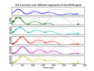
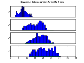
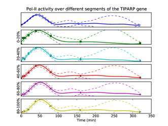
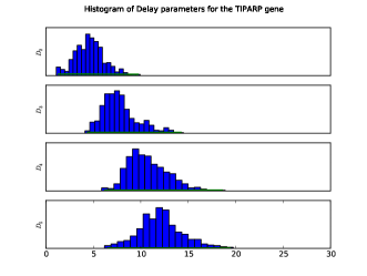
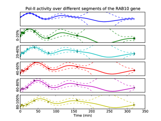
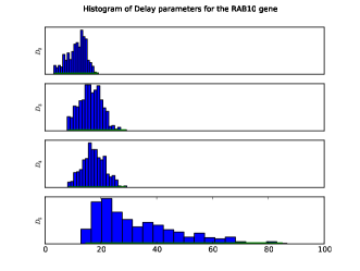
Figure 4: Inferred pol-II time profiles obtained for three of the top ten genes using ChIP-seq data. The top panel of each figure shows the inferred distribution of the latent funtion $f(t)$. The next five panels show the inferred profiles for the five gene segments corresponding to $0-20\%,\ldots,80\%-100\%$ of the gene. The figures on the right are the delay histograms

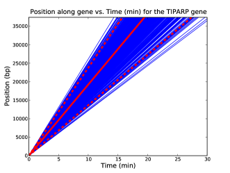
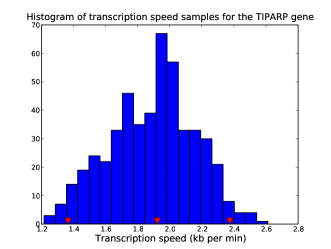
Figure 5: Linear regression plots using the delay samples for the TIPARP gene (a) and the histogram of speed samples (b). The 95% confidence interval is indicated in (a) by the dashed red lines with the median represented by the solid red line. In (b) the 95% confidence interval is indicated by the red triangle markers (cf. Table 5).

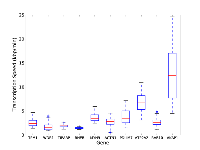
Figure 6: Box plot of speed estimates for the top ten genes found to fit the transcription model well.

Gene	Length (bp)	2.5%	50%	97.5%
TPM1	22196	1.6	2.4	4.1
WDR1	42611	1.0	1.6	3.5
TIPARP	32353	1.4	1.9	2.4
RHEB	53913	1.2	1.5	1.7
MYH9	106741	2.6	3.4	5.5
ACTN1	105244	0.6	2.8	4.2
PDLIM7	14208	1.7	3.5	6.4
ATP2A2	69866	3.6	6.8	10.2
RAB10	103595	1.4	2.6	4.4
AKAP1	36158	5.0	12.4	21.4

Table 5: Transcription speed in kilobases per minute for the top ten genes that fit the transcription model well. We use a Bayesian MCMC method for parameter estimation which provides the posterior distribution of the transcription speed. We show the 2.5%, 50% and 97.5% percentiles of the posterior distribution.

Gene	Length (bp)	2.5%	50%	97.5%
ACTN1	105244	0.6	2.8	4.2
ADCY1	148590	2.8	9.7	43.6
ARHGEF10L	158041	2.8	5.4	8.5
EPB41L1	120374	0.2	0.4	2.0
EPS15L1	110355	16.1	30.0	43.1
FARP1	102125	1.7	2.9	7.9
FLNB	163856	0.2	1.5	3.7
ITPK1	179005	0.3	2.9	6.8
JAK1	133282	0.6	2.2	4.2
JAK2	142939	0.6	2.4	5.3
KIAA0232	101441	0.9	2.3	4.0
KIF21A	150163	1.0	2.1	3.8
LARP1	104702	0.7	2.0	3.8
MYH9	106741	2.6	3.4	5.5
NCOR2	243050	6.5	10.9	20.5
NRIP1	103571	2.9	4.7	6.4
PKIB	116142	0.6	1.0	2.4
RAB10	103595	1.4	2.6	4.4
RAB31	154326	0.7	1.6	3.0
RASA3	150902	0.6	1.4	6.0
SHB	153316	0.5	3.1	5.0
WWC1	180244	1.9	3.6	5.6
ZNF644	106174	0.1	0.2	1.5

Table 6: Transcription speed in kilobases per minute for long genes between 100 and 300 kilobases long

Clustering of Promoter Activity Profiles

The inferred latent functions for each gene model the pol-II activity adjacent to the promoter. Clustering these profiles and examining the average profiles of each cluster allows us to visualise the general trends and also classify genes according to the immediacy and nature of the response. This provides an alternative to clustering based on mRNA abundance data (from microarray or RNA-Seq experiments) which is regulated both by mRNA production and degradation processes. The production of mRNA may be delayed relative to the actual activation of transcription at the promoter causing genes which are actually triggered at the same time to show different rates of mRNA production. Differences in degradation rate can also influence mRNA abundance profiles. It may therefore be difficult to distinguish early and delayed transcriptional regulation from mRNA abundance data.

To classify the profiles we sample the mean of the latent function ($f(t)$ in equation 1) and use PUMA-CLUST [30] to cluster the genes. PUMA-CLUST has the advantage of taking into account the uncertainty of the latent function when clustering the profiles. This uncertainty is computed from the posterior covariance of $f(t)$.

The 383 genes found to fit the model well were grouped into 12 clusters (Figure 7) with the optimal number of clusters determined by the Bayesian Information Criterion. To determine the speed of the response in each cluster, we compute the peak time of the mean profile for each cluster (see Table 7). We used the Genomatix Pathway System (GePS) to look for enriched canonical pathways ($p$-value $<0.01$) in each cluster (supplementary material, Table 14) and performed a Gene Ontology (GO) analysis of the clusters using the DAVID tool [31, 32] (supplementary material, Tables 15-LABEL:tab:DAVID_GO_3) showing that clusters are enriched for a number of different GO categories. The GO analysis identified early peaking clusters such as 2, 4 and 10 as enriched for nucleotide binding proteins consistent with many early genes being involved in downstream transcriptional regulation. The clustering of the pair of genes JAK1 and JAK2 in cluster 10, which has a prominent early peak, suggests that the response of both genes to E2 is rapid and coordinated. Since these genes are known to act together in several biological pathways such as the IL-6 signaling pathway and the IFN gamma signaling pathway, their appearance in the same cluster suggests that the clustering is likely to reveal other biologically significant relationships.

A closer look at the inferred pol-II promoter profiles of some examples in cluster 10, the earliest peaking cluster, and the corresponding inferred pol-II profiles over the last 20% of the genes reveals the possible influence of gene length on mRNA production and how clustering the inferred promoter profiles can account for this influence and uncover potential co-regulation. Figure 8 shows the inferred promoter profiles and the inferred pol-II profiles over the last 20% for three genes CLN8, BRI3BP and JAK2 in cluster 10. Figure 9 shows the corresponding raw ChIP-seq reads. The lengths of the genes to the nearest kilobase are 23, 32 and 143 kb respectively. We see that despite the last segment profiles peaking at different times, the promoter profiles peak at approximately the same time. The difference in peak time over the final segment of the gene is most likely due to the length of the genes and accounts for the amount of time the pol-II takes to move down the gene. Such differences would mask potential co-regulation if we attempted to cluster genes based on their mRNA profiles.

In Hah et al.  [3] GRO-seq was used to measure pol-II occupancy genome-wide when MCF-7 cells are treated with estradiol (E2) at four time points (0, 10, 40 and 160 min after E2 treatment). In addition, steady state levels of mRNA for 54 genes were measured using RT-qPCR at five time points (0, 10, 40, 160 and 320 min after E2 treatment). These data show a delay of between 1-3hr between peaks in the pol-II occupancy at the 5’ end of a gene and peaks in the mRNA steady state  [3, Figure S4]. These data include the mRNA measurement for 20 genes whose corresponding GRO-seq data peak is at 40 minutes after E2 treatment. Six of these genes namely CASP7, FHL2, GREB1, ITPK1, NRIP1, WWC1 are found to fit our pol-II model well with ChIP-seq data. Table 8 shows the peak time of the inferred promoter profile $T_{p}$, the peak time of the inferred pol-II profile over the last 20% of the gene $T_{\mathrm{last}}$, the GRO-seq peak time as well as the mRNA peak time. For the GRO-seq and mRNA peak times we show the peak times from Hah et al. [3, Figure S4] which are limited to the finite set of sampling times. We see that all mRNA peaks occur after $T_{\mathrm{last}}$. The large value of $T_{\mathrm{last}}$ for WWC1 which is a long gene $\sim 180$ kb in length corresponds to a late peak in mRNA at 320 minutes. This shows that the parameters obtained by our model are biologically plausible. Based solely on the GRO-seq data these genes were grouped together in  [3] since they show a peak at 40min. However our modeling reveals a greater diversity in the nature of responses. In fact the six genes appear in three different early response promoter profile clusters (see Table 8).

In the supplementary material, we compare the clustering obtained from the inferred promoter profiles to that obtained if the time series of the raw ChIP-seq reads are clustered and show that our model has the potential to uncover relationships which may be missed if we only consider the raw ChIP-seq reads.

Cluster	Peak Time (min)
1	48
2	32
3	61
4	32
5	100
6	58
7	80
8	122
9	242
10	22
11	297
12	80

Table 7: Cluster peak time

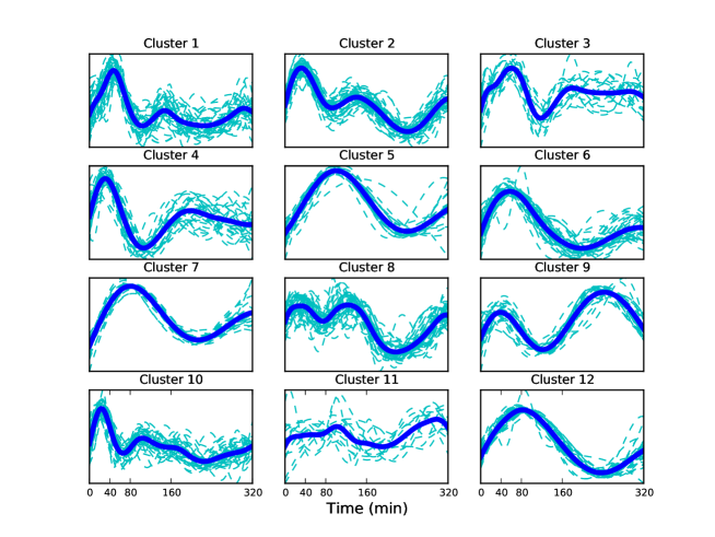
Figure 7: Clusters of promoter activity profiles. The mean profile in each cluster is shown by the bold line.

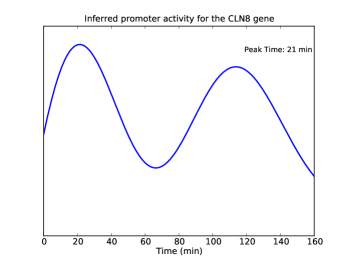
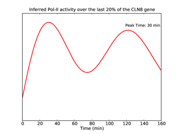
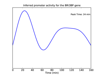
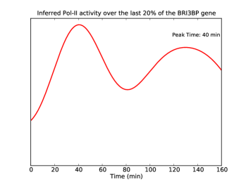
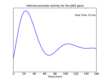
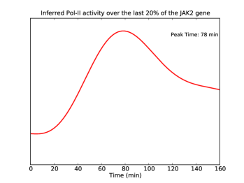
Figure 8: Inferred promoter profiles and pol-II activity over the final 20% of the gene for three genes in cluster 10.

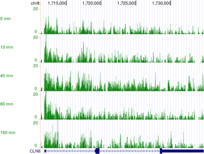
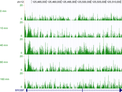
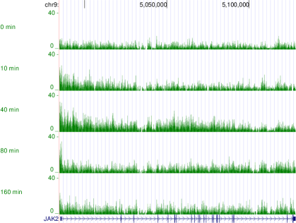
Figure 9: ChIP-seq reads for three genes in cluster 10: CLN8, BRI3BP and JAK2.

Gene	Cluster	$T_{p}$	$T_{20}$	GRO-seq Peak	mRNA Peak
CASP7	1	36	47	40	160
FHL2	1	42	55	40	160
GREB1	2	30	46	40	320
ITPK1	2	36	64	40	160
NRIP1	10	22	40	40	160
WWC1	10	23	81	40	320

Table 8: The peak time of the inferred promoter profile $T_{p}$, the peak time of the inferred pol-II profile over the last 20% of the gene $T_{20}$, the GRO-seq peak time as well as the mRNA peak time (from  [3, Figure S4]).

Transcription factor binding

We investigated the TF peaks in a 40 kbp region around the gene transcription start site for all genes in each cluster using ChIP-seq data for a number of TFs measured under similar experimental conditions (i.e. MCF-7 breast cancer cells treated with E2) in the cistrome database (http://cistrome.org). In earlier work on the estrogen interactome, Fullwood et al. [33] suggest that most long range interactions between TF binding sites and gene enhancers are limited to a range of about 20kb. We therefore investigate the region from -20kb to 20kb relative to the TSS (results for other regions around the TSS ranging from 1 to 100 kb are shown in the supplementary material (Tables 21 -24)). Table 9 shows the number of genes with TF binding peaks for each cluster for 7 TFs namely ER$\alpha$ [2], FoxA1 [34], c-Fos [35], c-Jun [35], c-MYC [36], SRC-3 [37], TRIM24 [38]. We found that the TFs RAD21 [39], CTCF [39] and STAG1 [39] are ubiquitously bound and not useful in uncovering cluster-specific TF binding. We investigate the statistical significance of the proportions of genes in each cluster with TF peaks in a 40kb neighborhood of the TSS by comparing the observed proportions to those we would expect in clusters of the same size drawn at random from the set of all genes. In Table 9 statistically significant ($p$-value $<0.05$) proportions are indicated in red (larger than expected) and green (lower than expected). For $p$-values less than $0.01$, the associated $p$-values are indicated in parentheses according to the following scale (***: $p<0.0001$,**: $p<0.001$,*:$p<0.01$).

Interestingly, clusters 1, 2, 4, and 10, which show an early peak in the mean promoter profile, are all enriched for ER$\alpha$ and FOXA1. These clusters, with the exception of cluster 4, were also found to be enriched for the ER$\alpha$ motif near the promoter. The enrichment of both ER$\alpha$ and FOXA1 in these clusters is in line with conclusions drawn in Hurtado et al. [40] where it was suggested FOXA1 mediates ER$\alpha$ binding. We also investigated the overlap of the binding sites for ER$\alpha$ and FOXA1 both in the 151 genes belonging to these clusters and genome-wide using the peaks obtained from [2] (ER$\alpha$) and [34] (FOXA1) and reported in the cistrome database. We investigated the 40kb region -20kbp to 20kbp relative to the TSS. Table 10 shows the number of ER$\alpha$ and FOXA1 peaks and the overlap (Two peaks are said to overlap if they have at least one base pair in common). We see that when we consider the rapid response genes in clusters 1, 2, 4, and 10 the percentage of overlap increases to 16% (35/220) whereas the overlap is 9% (956/11056) when we consider all genes. The significance associated with this elevated overlap is p=0.004 given the null hypothesis of a random gene list of the same size (results for other regions around the TSS ranging from 1 to 100 kb are shown in the supplementary material (Tables 25 -28))). Taken together, the results in Tables 9 and 10 identify genes that respond to E2, with clusters 1, 2, 4 and 10 most likely to contain the earliest estrogen responsive genes.

Cluster	TFs
	ER$\alpha$	FOXA1	c-FOS	c-JUN	MYC	SRC-3	TRIM24
1 (37)	27 (**)	14	16 (*)	6	4	25 (*)	27
2 (47)	31 (*)	19 (*)	16	7	7	36 (***)	38
3 (18)	11	5	7	5	6 (**)	11	12
4 (29)	20 (*)	11	9	7	2	18	23
5 (27)	15	4	6	8 (*)	9 (***)	16	19
6 (40)	27 (*)	8	12	7	4	25	31
7 (24)	10	6	5	6	3	13	19
8 (47)	32 (*)	10	14	14 (**)	8	31 (*)	40 (*)
9 (26)	18	7	11 (*)	11 (***)	3	12	22
10 (38)	30 (***)	14	15 (*)	2	1	29 (**)	32 (*)
11 (13)	5	2	7 (*)	4	2	7	13 (*)
12 (37)	19	8	12	11 (**)	4	23	29

Table 9: Analysis of transcription factor binding in 40kbp regions of genes in gene clusters obtained from inferred promoter activity profiles. The number in parentheses in the first column is the cluster size. For each TF, we show the number of genes with peaks. Statistically significant proportions ($p$-value $<0.05$) are indicated in red (larger than expected). For $p$-values less than $0.01$, the associated $p$-values are indicated in parentheses according to the following scale (***: $p<0.0001$,**: $p<0.001$,*:$p<0.01$).

Genes	# of ER$\alpha$ peaks	# of FOXA1 peaks	ER$\alpha$ and FOXA1 overlap
Clusters 1, 2, 4, and 10 (151)	220 (112)	86 (44)	35 (0.004)
All genes ($\sim$ 20,000)	11056	4626	956

Table 10: Overlap of ER$\alpha$ and FOXA1 binding in a 40 kb region around the TSS. The numbers in parentheses in the first column are the number of genes. In each TF peak column, we show the expected number of peaks in a set of random random genes of the same size in parentheses. In the overlap column the associated p-value is shown in parentheses.

Discussion

In this work we have presented a methodology for modelling transcription dynamics and employed it to determine the transcriptional response of breast cancer cells to estradiol. To capture the movement of pol-II down the gene body, we model the observed pol-II occupancy time profiles over different gene segments as the delayed response of linear systems to the same input. The input is assumed to be drawn from a Gaussian process which models the pol-II activity adjacent to the gene promoter. Given observations from high-throughput data such as pol-II ChIP-Seq data, we are able to infer this input function and estimate the pol-II activity at the promoter. This allows us to differentiate transcriptionally engaged pol-II from pol-II paused at the promoter and yields good estimates of transcriptional activity.

In addition to estimating the transcriptional activity at the promoter, inferring the pol-II occupancy time profiles over different gene segments allows us to compute the transcription speed. We expect the delay parameters of different gene segments to be non-decreasing and this provides a natural way to determine genes that are being actively transcribed in response to E2.

Clustering the inferred promoter activity profiles allows us to investigate the nature of the response and group genes that are likely to be co-regulated. We found that the four clusters significantly enriched for both ER$\alpha$ and FOXA1 binding within 40kb according to public ChIP-Seq data were those that showed the earliest peak in pol-II activity at the promoter. ER$\alpha$ and FOXA1 ChIP peaks in the neighbourhood of these genes were also more likely to be overlapping than the average for ChIP-identified binding events of these TFs genome-wide. This observation provides some support for the previously proposed role of FOXA1 as a mediator of early transcriptional response in estrogen signalling. These results also show that our method can help regulatory network inference. The inferred promoter activity profiles pinpoint the times of transcriptional activation very accurately without confounding transcriptional delays. As genes with similar inferred promoter activity profiles are likely to have similar TF binding profiles, they are likely to be co-regulated as well. The promoter profiles should therefore lead to more accurate predictions of regulator-target relationships using time-course-based methods (e.g. [9]) than using expression time course data.

As well as modelling transcriptional speed and transcriptional activity profiles, the proposed modelling approach may have other useful applications. For example, recent research has uncovered a link between transcription dynamics and alternative splicing [41]. It is believed that aberrant splicing can cause disease and a number of studies have tried to understand the mechanisms of alternative splicing [42]. The proposed model can potentially be used to identify transcriptional pausing events, and such results could be usefully combined with inference of splice variation from RNA-Seq datasets from the same system. Also, with the increasing availability of high-throughput sequencing data exploring multiple layered views of the transcription process and its regulation, the convolved modelling approach developed here has the potential to be usefully applied to more complex coupled spatio-temporal datasets.

Supplementary information

Priors

The parameters $\Theta=\{\sigma_{f},\ell_{f},\{\alpha_{i},D_{i},\ell_{i},\sigma_{i}\}_{i=1}^{I}\}$ are positive and bounded. In the experiments we use the bounds shown in Table 11 with $D_{1}$ fixed at zero, $\sigma_{f}=1$ and the values $\sigma_{i}$ tied to single value. To determine the delay bounds, we assume that the value of $D_{i}$ is an indicator of how long it takes the ‘transcription wave’ to reach the corresponding gene segment. That is $D_{2}$ is the amount of time it takes to transcribe 20% of the gene, $D_{3}$ 40% etc. We obtain the length $L$ of the gene from the hg19 annotation and use values of maximum and minimum expected speed ($s_{min}$ and $s_{max}$ respectively) to compute the delay bound. For example

$$D_{2}^{min}=\frac{0.2L}{s_{max}}\quad\mathrm{and}\quad D_{2}^{max}=\frac{0.2L}{s_{min}}$$

We use $s_{min}=50$ bp min^-1 and $s_{max}=50$ kbp min^-1. These large bounds allow unbiased estimation of transcription speed. (Recent work on individual cells suggests speeds as high as 50kb per minute are possible [43].)

We transform the parameters using a logit transform and work with unconstrained variables. For a parameter $\theta\in\Theta$ with corresponding minimum and maximum bounds $\theta_{min}$ and $\theta_{max}$ respectively we compute the transfromed variable $\gamma$

$$\gamma=\log\Big{(}\frac{\theta-\theta_{min}}{\theta_{max}-\theta}\Big{)}.$$ (14)

We place a Gaussian prior over the parameters in the transformed domain and draw samples from the posterior using the Hamiltonian Monte Carlo (HMC) algorithm [21]. We have

$$\gamma\sim\mathcal{N}(\gamma|0,\sigma_{\gamma}).$$ (15)

With $,\sigma_{\gamma}=2$ we obtain an approximately uniform prior in the untransformed domain yielding an uninformative prior.

Parameter	Minimum	Maximum
$\ell_{f}$	5 min	320 min
$\alpha_{i}$	0	100
$D_{i}$	$\frac{0.2(i-1)L}{s_{max}}$ min	$\frac{0.2(i-1)L}{s_{min}}$ min
$\ell_{f}$	5 min	320 min
$\sigma_{i}$	0	100

Table 11: Parameter bounds.

To initialise the parameters for gradient optimisation, the length scales $\ell_{f}$ and $\ell_{i}$ are initilised at random from $\{10,20,30,40,80\}$, $\alpha_{i}$ and $\sigma_{i}$ are drawn from $\mathcal{U}[0,1]$ with the value of $\sigma_{i}$ multiplied by 100 to avoid local minima that would under-estimate the variance. The delays are inilialised at random with the more realistic speed bounds $s_{min}$=500 bp per min and $s_{max}$ = 5kb per min when an ensemble of cells is considered. The parameters are then freely optimised with the bounds given in Table 11.

Parameter gradients

To obtain ML estimates of the parameters we maximise the log marginal likelihood. To do this we require the gradients of the covariance function w.r.t the parameters. The gradients w.r.t $\alpha_{i}$ and $\sigma_{i}$ are straight forward. Here we give the expressions for the gradients of $\mathsf{cov}[y_{i}(t),y_{j}(t^{\prime})]=K_{yy}$ w.r.t $\ell_{f}$, $\ell_{i}$ and $D_{i}$. We have

$$\frac{\partial K_{yy}}{\partial\ell_{f}} = \alpha_{i}\alpha_{j}\frac{\sigma_{f}^{2}(\ell_{i}^{2}+\ell_{j}^{2})}{(\ell_{f}^{2}+\ell_{i}^{2}+\ell_{j}^{2})^{\frac{3}{2}}}\exp\Bigg{(}-\frac{(t^{\prime}-t+D_{i}-D_{j})^{2}}{2(\ell_{f}^{2}+\ell_{i}^{2}+\ell_{j}^{2})}\Bigg{)}$$ (16)

$$+ \alpha_{i}\alpha_{j}\frac{\sigma_{f}^{2}\ell_{f}}{\sqrt{\ell_{f}^{2}+\ell_{i}^{2}+\ell_{j}^{2}}}\exp\Bigg{(}-\frac{(t^{\prime}-t+D_{i}-D_{j})^{2}}{2(\ell_{f}^{2}+\ell_{i}^{2}+\ell_{j}^{2})}\Bigg{)}\frac{(t^{\prime}-t+D_{i}-D_{j})^{2}}{(\ell_{f}^{2}+\ell_{i}^{2}+\ell_{j}^{2})^{2}}$$

$$\frac{\partial K_{yy}}{\partial\ell_{i}} = -\alpha_{i}\alpha_{j}\frac{\sigma_{f}^{2}\ell_{f}\ell_{i}}{(\ell_{f}^{2}+\ell_{i}^{2}+\ell_{j}^{2})^{\frac{3}{2}}}\exp\Bigg{(}-\frac{(t^{\prime}-t+D_{i}-D_{j})^{2}}{2(\ell_{f}^{2}+\ell_{i}^{2}+\ell_{j}^{2})}\Bigg{)}$$ (17)

$$+ \alpha_{i}\alpha_{j}\frac{\sigma_{f}^{2}\ell_{f}}{\sqrt{\ell_{f}^{2}+\ell_{i}^{2}+\ell_{j}^{2}}}\exp\Bigg{(}-\frac{(t^{\prime}-t+D_{i}-D_{j})^{2}}{2(\ell_{f}^{2}+\ell_{i}^{2}+\ell_{j}^{2})}\Bigg{)}\frac{\ell_{i}(t^{\prime}-t+D_{i}-D_{j})^{2}}{(\ell_{f}^{2}+\ell_{i}^{2}+\ell_{j}^{2})^{2}}$$

$$\frac{\partial K_{yy}}{\partial D_{i}}=-\alpha_{i}\alpha_{j}\frac{\sigma_{f}^{2}\ell_{f}}{\sqrt{\ell_{f}^{2}+\ell_{i}^{2}+\ell_{j}^{2}}}\exp\Bigg{(}-\frac{(t^{\prime}-t+D_{i}-D_{j})^{2}}{2(\ell_{f}^{2}+\ell_{i}^{2}+\ell_{j}^{2})}\Bigg{)}\frac{(t^{\prime}-t+D_{i}-D_{j})}{(\ell_{f}^{2}+\ell_{i}^{2}+\ell_{j}^{2})}$$ (18)

To obtain gradient w.r.t the transformed parameters given by equation 14, we employ the chain rule.

$$\frac{\partial K_{yy}}{\partial\gamma} = \frac{\partial K_{yy}}{\partial\theta}\frac{\partial\theta}{\partial\gamma}$$ (19)

$$= \frac{\partial K_{yy}}{\partial\theta}\frac{\exp(\gamma)(\theta_{max}-\theta_{min})}{(1+\exp(\gamma))^{2}}$$

Canonical Pathway and Gene Ontology Analysis

To determine the biological significance of the 383 genes found to fit the pol-II dynamics model well, we used the Genomatix Pathway System (GePS) to look for enriched canonical pathways and gene ontology categories. Table 12 shows the significant canonical pathways ($p$-value $<0.05$) and the observed genes. It is interesting to note that the pair of genes JAK1 and JAK2 are responsible for a large number of the significant canonical pathways. These genes have previously been suggested as potential drug targets in breast cancer (see for example [44]). The enrichment of the FOXA1 transcriptional network provides further confirmation that our model identifies biologically relevant genes. In recent work, Hurtado et al. [40] showed that FOXA1 influences the interaction of ER$\alpha$ and chromatin and therefore influences the response of breast cancer cells to E2. Genes in the FOXA1 canonical network found to fit the pol-II model well include NRIP1 which is believed to be a direct E2 target that mediates the repression of ER$\alpha$ target genes later in the time course[45, 46]. Table 13 shows the top 20 significant gene ontology terms ($p$-value $<0.05$) for molecular function.

Canonical pathway	Genes
IL-6 signaling pathway(JAK1 JAK2 STAT3)	JAK1, JAK2
IFN gamma signaling pathway	JAK1, JAK2
Proteasome complex	PSME1, PSMA4, PSMB5, PSMA2
IL-3 signaling pathway(JAK1 JAK2 STAT5)	JAK1, JAK2
Stat3 signaling pathway	JAK1, JAK2
FOXA1 transcription factor network	AP1B1, NDUFV3, NRIP1, SHH
PDGFR-alpha signaling pathway	JAK1, PDGFB, SHB
Hypoxia and p53 in the cardiovascular system	FHL2, HIF1A, GADD45A
LIF signaling pathway	JAK1, JAK2
IL-5 signaling pathway	JAK1, JAK2
p53 signaling pathway	TIMP3, GADD45A
IL-10 anti-inflammatory signaling pathway	JAK1, BLVRB
AndrogenReceptor	SPDEF, FHL2, STUB1
	NCOR2, NRIP1
Integrin signaling pathway	CSK, ACTN1, NOLC1
Erythropoietin mediated
neuroprotection through NF-KB	HIF1A, JAK2
PDGFR-beta signaling pathway	ACTR2, HCK, CSK,
	PDGFB, CTTN, JAK2
Mechanisms of transcriptional
repression by dna methylation	RBBP7, MBD1
Hypoxia-inducible factor in
the cardivascular system	HIF1A, LDHA

Table 12: Significant canonical pathways ($p$-value $<0.05$) for the 383 genes found to fit the pol-II dynamics model well.

Molecular function
Structural constituent of ribosome
RNA binding
Methyl-CpG binding
Protein binding
Structural molecule activity
Nucleic acid binding
rRNA binding
Non-membrane spanning protein tyrosine kinase activity
Ribosomal small subunit binding
Pseudouridine synthase activity
S100 alpha binding
Growth hormone receptor binding
Isomerase activity
Glucocorticoid receptor binding
Translation factor activity, nucleic acid binding
NF-kappaB binding
Threonine-type peptidase activity
Threonine-type endopeptidase activity
Intramolecular transferase activity

Table 13: Top 20 significant gene ontology terms ($p$-value $<0.05$) for the 383 genes found to fit the pol-II dynamics model well.

Table 14 shows the significant canonical pathways ($p$-value $<0.01$) and the observed genes in each of the 12 promoter profile clusters. We also perform a gene ontology analysis of the 12 promoter profile clusters using the DAVID tool from the NIH [31, 32]. The enriched gene ontology categories ($p$-value $<0.05$) are shown in Table 15, (for molecular function), Table LABEL:tab:DAVID_GO_2 (for biological processes) and Table LABEL:tab:DAVID_GO_3 (for cellular components).

Cluster	Canonical pathway	Genes
1 (37)	PDGFR-beta signaling pathway	PDGFB, ACTR2, HCK
2 (47)	-	-
3 (18)	-	-
4 (29)	Nuclear receptors coordinate the activities	NCOR2, TAF5
	of chromatin remodeling complexes and coactivators
	to facilitate initiation of transcription in carcinoma cells
5 (27)	-	-
6 (40)	-	-
7 (24)	Proteasome complex	PSMB5, PSME1
	Antigen processing and presentation	PSMB5
8 (47)	-	-
9 (26)	-	-
10 (38)	IFN gamma signaling pathway	JAK2, JAK1
	IL-6 signaling pathway	JAK2, JAK1
	IL-3 signaling pathway	JAK2, JAK1
	Stat3 signaling pathway	JAK2, JAK1
	LIF signaling pathway	JAK2, JAK1
	IL-5 signaling pathway	JAK2, JAK1
	PDGFR-alpha signaling pathway	SHB, JAK1
	IL27-mediated signaling events	JAK2, JAK1
	Role of ErbB2 in signal transduction and oncology	JAK2, JAK1
	IL6-mediated signaling events	JAK2, JAK1
	JAK_STAT_MolecularVariation_2	JAK2, JAK1
11 (13)	-	-
12 (37)	-	-

Table 14: Pathway analysis of clusters from inferred promoter activity profiles. The number in parentheses in column 1 is the cluster size.

Cluster	GO ID	GO TERM
1 (37)	GO:0008092	Cytoskeletal protein binding
	GO:0003779	Actin binding
	GO:0005085	Guanyl-nucleotide exchange factor activity
2 (47)	GO:0003723	RNA binding
3 (18)	-	-
4 (29)	GO:0003723	RNA binding
	GO:0030528	transcription regulator activity
	GO:0003677	DNA binding
	GO:0003700	Transcription factor activity
5 (27)	-	-
6 (40)	GO:0003735	Structural constituent of ribosome
7 (24)	GO:0003735	Structural constituent of ribosome
	GO:0005198	Structural molecule activity
	GO:0003723	RNA binding
8 (47)	-	-
9 (26)	GO:0043021	Ribonucleoprotein binding
10 (38)	GO:0005131	Growth hormone receptor binding
	GO:0051427	Hormone receptor binding
	GO:0032553	Ribonucleotide binding
	GO:0032555	Purine ribonucleotide binding
	GO:0017076	Purine nucleotide binding
	GO:0005525	GTP binding
	GO:0019001	Guanyl nucleotide binding
	GO:0032561	Guanyl ribonucleotide binding
	GO:0004713	Protein tyrosine kinase activity
11 (13)	-	-
12 (37)	GO:0003735	Structural constituent of ribosome
	GO:0005198	Structural molecule activity
	GO:0003723	RNA binding

Table 15: Enriched gene ontology categories for molecular function ($p$-value $<0.05$) of clusters from inferred promoter activity profiles. The number in parentheses in column 1 is the cluster size.

Table 16: Enriched gene ontology categories for biological processes ($p$-value $<0.05$) of clusters from inferred promoter activity profiles. The number in parentheses in column 1 is the cluster size.

Cluster	GO ID	GO TERM
1 (37)	GO:0030036	Actin cytoskeleton organization
	GO:0030029	Actin filament-based process
	GO:0007010	Cytoskeleton organization
	GO:0007517	Muscle organ development
	GO:0001503	Ossification
	GO:0001501	Skeletal system development
	GO:0060348	Bone development
	GO:0060537	Muscle tissue development
	GO:0051496	Positive regulation of stress fiber formation
	GO:0007167	Enzyme linked receptor protein signaling pathway
	GO:0045935	Positive regulation of nucleobase,
		nucleoside, nucleotide and nucleic acid metabolic process
	GO:0032233	Positive regulation of actin filament bundle formation
	GO:0051173	Positive regulation of nitrogen compound metabolic process
	GO:0010557	Positive regulation of macromolecule biosynthetic process
	GO:0031328	Positive regulation of cellular biosynthetic process
	GO:0009891	Positive regulation of biosynthetic process
	GO:0051492	Regulation of stress fiber formation
	GO:0048008	Platelet-derived growth factor receptor signaling pathway
	GO:0032231	Regulation of actin filament bundle formation
	GO:0055010	Ventricular cardiac muscle morphogenesis
	GO:0055008	Cardiac muscle tissue morphogenesis
	GO:0060415	Muscle tissue morphogenesis
2 (47)	GO:0051272	Positive regulation of cell motion
	GO:0043085	Positive regulation of catalytic activity
	GO:0044093	Positive regulation of molecular function
3 (18)	GO:0006364	rRNA processing
	GO:0016072	rRNA metabolic process
4 (29)	GO:0010558	Negative regulation of macromolecule biosynthetic process
	GO:0031327	Negative regulation of cellular biosynthetic process
	GO:0006350	Transcription
	GO:0009890	Negative regulation of biosynthetic process
	GO:0010605	Negative regulation of macromolecule metabolic process
	GO:0016481	Negative regulation of transcription
	GO:0010629	Negative regulation of gene expression
	GO:0045934	Negative regulation of nucleobase,
		nucleoside, nucleotide and nucleic acid metabolic process
	GO:0051172	Negative regulation of nitrogen compound metabolic process
5 (27)	-	-
6 (40)	GO:0048147	Negative regulation of fibroblast proliferation
	GO:0022613	Ribonucleoprotein complex biogenesis
7 (24)	GO:0019941	Modification-dependent protein catabolic process
	GO:0043632	Modification-dependent macromolecule catabolic process
	GO:0051603	Proteolysis involved in cellular protein catabolic process
	GO:0044257	Cellular protein catabolic process
	GO:0030163	Protein catabolic process
	GO:0006412	Translation
	GO:0043161	Proteasomal ubiquitin-dependent protein catabolic process
	GO:0010498	Proteasomal protein catabolic process
	GO:0044265	Cellular macromolecule catabolic process
	GO:0009057	Macromolecule catabolic process
	GO:0006508	Proteolysis
	GO:0006511	Ubiquitin-dependent protein catabolic process
8 (47)	GO:0042273	Ribosomal large subunit biogenesis
	GO:0006396	RNA processing
	GO:0006400	tRNA modification
9 (26)	GO:0043086	Negative regulation of catalytic activity
10 (38)	GO:0007242	Intracellular signaling cascade
	GO:0015031	Protein transport
	GO:0045184	Establishment of protein localization
	GO:0008104	Protein localization
	GO:0001525	Angiogenesis
	GO:0010876	Lipid localization
11 (13)	-	-
12 (37)	GO:0006412	Translation
	GO:0006414	Translational elongation
	GO:0051168	Nuclear export
	GO:0042274	Ribosomal small subunit biogenesis
	GO:0000278	Mitotic cell cycle
	GO:0006974	Response to DNA damage stimulus
	GO:0006913	Nucleocytoplasmic transport
	GO:0051169	Nuclear transport
	GO:0022613	Ribonucleoprotein complex biogenesis

Table 17: Enriched gene ontology categories for cellular components ($p$-value $<0.05$) of clusters from inferred promoter activity profiles. The number in parentheses in column 1 is the cluster size.

Cluster	GO ID	GO TERM
1 (37)	GO:0015629	Actin cytoskeleton
	GO:0005856	Cytoskeleton
	GO:0043228	Non-membrane-bounded organelle
	GO:0043232	Intracellular non-membrane-bounded organelle
	GO:0030017	Sarcomere
	GO:0030016	Myofibril
	GO:0044449	Contractile fiber part
	GO:0043292	Contractile fiber
	GO:0001725	Stress fiber
2 (47)	-	-
3 (18)	-	-
4 (29)	GO:0016604	Nuclear body
	GO:0005654	Nucleoplasm
	GO:0030529	Ribonucleoprotein complex
	GO:0044451	Nucleoplasm part
	GO:0031981	Nuclear lumen
	GO:0022625	Cytosolic large ribosomal subunit
5 (27)	GO:0030529	Ribonucleoprotein complex
	GO:0005732	Small nucleolar ribonucleoprotein complex
	GO:0043232	Intracellular non-membrane-bounded organelle
	GO:0043228	Non-membrane-bounded organelle
6 (40)	GO:0044429	Mitochondrial part
	GO:0070013	Intracellular organelle lumen
	GO:0043233	Organelle lumen
	GO:0031974	Membrane-enclosed lumen
	GO:0005743	Mitochondrial inner membrane
	GO:0019866	Organelle inner membrane
	GO:0044455	Mitochondrial membrane part
	GO:0033279	Ribosomal subunit
	GO:0031966	Mitochondrial membrane
	GO:0005739	Mitochondrion
	GO:0005740	Mitochondrial envelope
	GO:0005840	Ribosome
7 (24)	GO:0005840	Ribosome
	GO:0033279	Ribosomal subunit
	GO:0030529	Ribonucleoprotein complex
	GO:0000313	Organellar ribosome
	GO:0005761	Mitochondrial ribosome
8 (47)	GO:0031981	Nuclear lumen
	GO:0005730	Nucleolus
	GO:0070013	Intracellular organelle lumen
	GO:0043233	Organelle lumen
	GO:0031974	Membrane-enclosed lumen
	GO:0030529	Ribonucleoprotein complex
9 (26)	GO:0031981	Nuclear lumen
10 (38)	GO:0009898	Internal side of plasma membrane
	GO:0044459	Plasma membrane part
11 (13)	GO:0022625	Cytosolic large ribosomal subunit
	GO:0015934	Large ribosomal subunit
	GO:0022626	Cytosolic ribosome
12 (37)	GO:0005840	Ribosome
	GO:0033279	Ribosomal subunit
	GO:0030529	Ribonucleoprotein complex
	GO:0043232	Intracellular non-membrane-bounded organelle
	GO:0043228	Non-membrane-bounded organelle
	GO:0044445	Cytosolic part
	GO:0005761	Mitochondrial ribosome
	GO:0000313	Organellar ribosome
	GO:0015935	Small ribosomal subunit
	GO:0015934	Large ribosomal subunit
	GO:0031980	Mitochondrial lumen
	GO:0005759	Mitochondrial matrix
	GO:0022626	Cytosolic ribosome
	GO:0005829	Cytosol
	GO:0070013	Intracellular organelle lumen
	GO:0043233	Organelle lumen
	GO:0031974	Membrane-enclosed lumen
	GO:0005739	Mitochondrion
	GO:0000315	Organellar large ribosomal subunit
	GO:0005762	Mitochondrial large ribosomal subunit

Clustering the raw ChIP-Seq reads

Pol-II occupancy in the proximal promoter region -250 bp to +750 bp relative to the transcription start site (TSS) was computed in RPM for the 383 genes and the time series grouped into 12 clusters. The clusters are shown in Figure 10. Table 18 shows the significant canonical pathways ($p$-value $<0.01$) and the observed genes in each of the 12 clusters. We find that in this case JAK1 and JAK2 appear in different clusters which have diffent temporal profiles. This may be due to the noisy nature of the data and the inclusion of paused pol-II in the proximal region time series. Our model which has the potential to uncover the signal due to pol-II that is engaged in transcription could be useful in uncovering relationships which may be missed if we only consider the raw ChIP-seq reads.

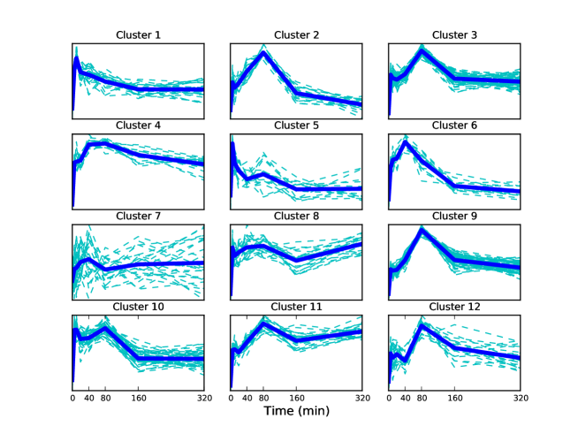
Figure 10: Clusters of promoter activity profiles derived directly from the raw ChIP-seq reads. The mean profile in each cluster is shown by the bold line.

Cluster	Canonical pathway	Genes
1 (24)	Transcriptional activation of dbpB from mRNA	PDGFB
2 (23)	-	-
3 (75)	Hypoxia and p53 in the cardiovascular system	GADD45A, HIF1A
4 (18)	Generation of amyloid b-peptide by ps1	ATP5G3
5 (16)	PDGFR-alpha signaling pathway	SHB, JAK1
	IFN gamma signaling pathway	JAK1
	IL-6 signaling pathway	JAK1
	IL-10 signaling pathway	JAK1
6 (15)	-	-
7 (24)	-	-
8 (24)	-	-
9 (67)	Proteasome complex	PSME1, PSMB5, PSMA4
10 (49)	TPO signaling pathway	JAK2
11 (29)	Glypican 3 network	SHH
	Sonic hedgehog receptor ptc1 regulates cell cycle	SHH
12 (19)	Hypoxia-inducible factor in the cardivascular system	LDHA
	Fibrinolysis pathway	ATP2A2

Table 18: Pathway analysis of clusters from raw ChIP-seq reads in the proximal promoter region -250bp to +750bp from the TSS. The number in parentheses in column 1 is the cluster size.

Transcription Factor Binding

Motifs

Tullai et al. [47] investigated genes that are co-regulated by shared transcription factor binding sites (TFBS). In particular, they found certain TFBS were enriched in the promoters of early response genes. We therefore investigated whether the promoters of genes in the different promoter profile clusters are enriched for different TFs. We use Pscan [48] to look for enriched TF motifs among those available in JASPAR [49]. The proximal promoter region -450 bp to +50 bp relative to the TSS of the genes in each cluster was analyzed. Table 19 shows signifiantly enriched TFBS in each cluster ($p$-value $<0.05$). Shown are TFs whose binding sites are over-represented in at least 5 clusters. The estrogen response element (ERE) is enriched in five clusters (1, 2, 5, 6 and 10), indicating that our modelling identifies estrogen responsive regions. The clusters containing an ERE have mean promoter activity profiles with distinct early peaks followed by decrease in activity which suggests transient activity. Additionally, clusters 1, 2 and 10 have relatively early peaks.

TF	Cluster
	1	2	3	4	5	6	7	8	9	10	11	12
GABPA	$\checkmark$	$\checkmark$	$\checkmark$	$\checkmark$	$\checkmark$	-	$\checkmark$	$\checkmark$	$\checkmark$	-	$\checkmark$	$\checkmark$
Zfx	$\checkmark$	$\checkmark$	-	$\checkmark$	$\checkmark$	-	-	$\checkmark$	$\checkmark$	$\checkmark$	$\checkmark$	$\checkmark$
Klf4	$\checkmark$	$\checkmark$	-	$\checkmark$	-	-	$\checkmark$	$\checkmark$	$\checkmark$	$\checkmark$	-	$\checkmark$
ELK1	$\checkmark$	-	-	$\checkmark$	$\checkmark$	-	$\checkmark$	$\checkmark$	$\checkmark$	-	$\checkmark$	$\checkmark$
HIF1A::ARNT	$\checkmark$	$\checkmark$	-	$\checkmark$	$\checkmark$	$\checkmark$	$\checkmark$	-	-	$\checkmark$	$\checkmark$	-
ELK4	$\checkmark$	-	$\checkmark$	$\checkmark$	$\checkmark$	-	$\checkmark$	$\checkmark$	$\checkmark$	-	-	$\checkmark$
SP1	$\checkmark$	$\checkmark$	-	$\checkmark$	-	-	-	$\checkmark$	$\checkmark$	$\checkmark$	-	$\checkmark$
TFAP2A	$\checkmark$	$\checkmark$	-	$\checkmark$	-	$\checkmark$	-	$\checkmark$	-	$\checkmark$	-	-
Mycn	$\checkmark$	-	-	$\checkmark$	$\checkmark$	-	-	$\checkmark$	-	$\checkmark$	$\checkmark$	-
Myc	$\checkmark$	-	-	$\checkmark$	$\checkmark$	-	-	$\checkmark$	-	$\checkmark$	$\checkmark$	-
Pax5	$\checkmark$	$\checkmark$	-	$\checkmark$	-	-	-	-	-	$\checkmark$	-	$\checkmark$
ER$\alpha$	$\checkmark$	$\checkmark$	-	-	$\checkmark$	$\checkmark$	-	-	-	$\checkmark$	-	-
Arnt::Ahr	-	$\checkmark$	-	$\checkmark$	-	-	$\checkmark$	$\checkmark$	-	$\checkmark$	-	-

Table 19: Significantly over-represented ($p$-value $<0.05$) transcription factor binding sites in the promoter profile clusters. We use Pscan to look for enriched TF motifs among those available in JASPAR. The proximal promoter region -450 bp to +50 bp relative to the TSS of the genes in each cluster was analyzed.

Next we investigated the EREs in the genes belonging to the 5 clusters enriched for the ERE motif. For each promoter sequence, the best sequence match to the ERE position frequency matrix (PFM) in JASPAR (MA0112.2) was determined. We keep those sequences with a matrix score greater than the mean score for matches found in the promoter sequences over the whole genome (For the ERE PFM this value is $0.73$ when we consider the region -450 bp to +50 bp relative to the TSS). We used these sequences to determine the consensus ERE motif in this group of genes. To determine the consensus sequence, we report a single nucleotide for a given position if the nucleotide has a frequency greater than 50% and a frequency twice as large as the next nucleotide. We obtain a consensus sequence of 5’-GGnCACCCTGnCC-3’ (where n is any nucleotide) and an average matrix score of 0.77. The sequence is visualised in Figure 11 (A). The sequence of the ERE is known and given as 5’-GGTCAnnnTGACC-3’ [50, 51]. The sequence corresponding to the PFM MA0112.2 is visualised in Figure 11 (B). We see that the ERE motif we obtain agrees well with the known motif.

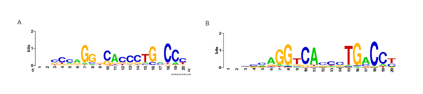
Figure 11: Consensus sequence of regions matching the ERE motif in the promoter profile clusters enriched for the ERE motif (A) and the Estrogen Response Element (B).

Table 20 shows the EREs in each of the 5 clusters visualised using WebLogo. We also show the consensus sequence and the average matrix score. To determine the consensus sequence, we report a single nucleotide for a given position if the nucleotide has a frequency greater than 50% and a frequency twice as large as the next nucleotide. We see that there is some diversity in the motifs correspoding to different clusters but the consensus sequences agree with the known motif. Differences appear at at most 3 positions with the consensus sequence for cluster 10 differing at only two positions. We see that for the half site ‘TGACC’ the ‘A’ does not appear in the consensus sequence in all the clusters.

Cluster	ERE Motif	Consensus sequence	Average Matrix
			Score
1		GnnCACCCTGnCCC	0.772
2		GGnnACCCTGnCCn	0.77
5		GGnnAnCCTGnCCn	0.761
6		GGnnACCnTGnCCn	0.762
10		GGnCACCCTGnCCn	0.765

Table 20: Analysis of the ERE in promoter regions of gene clusters obtained from inferred promoter activity profiles. The EREs in each of the 5 clusters are visualised using WebLogo (http://weblogo.berkeley.edu/). The consensus sequence is shown from postion 7 which corresponds to the known ERE motif. The average matrix score is computed using the sequence matrix scores from Pscan.

Transcription factor binding

Determining the TFBS motifs enriched in each cluster provides a way to determine the influence of TFs on transcription. As a complementary approach, we also investigated the TF peaks in regions ranging from 1 to 100 kb around the gene transcription start site for all genes in each cluster using ChIP-seq data for a number of TFs measured under similar experimental conditions (i.e. MCF-7 breast cancer cells treated with E2) in the cistrome database (http://cistrome.org).

Tables 21 to 24 show the number of genes with TF binding peaks for regions around the TSS ranging from 1 to 100 kb for each cluster for 7 TFs namely ER$\alpha$ [2], FoxA1 [34], c-Fos [35], c-Jun [35], c-MYC [36], SRC-3 [37], TRIM24 [38]. In the tables, statistically significant ($p$-value $<0.05$) proportions are indicated in red (larger than expected) and green (lower than expected) with associated $p$-values in parentheses. These p-values are obtained empirically by drawing 1e6 samples from a hypergeometric distribution.

We investigated the overlap of the binding sites for ER$\alpha$ and FOXA1 both in the 151 genes belonging to the rapid response genes in clusters 1, 2, 4, and 10 and genome-wide using the peaks obtained from [2] (ER$\alpha$) and [34] (FOXA1) and reported in the cistrome database. We investigated regions around the TSS ranging from 2 to 100 kb. Tables 25-28 show the number of ER$\alpha$ and FOXA1 peaks and the overlap. The statistical significance is determined by comparing the overlap in random gene lists of the same size.

Cluster	TFs
	ER$\alpha$	FOXA1	c-FOS	c-JUN	MYC	SRC-3	TRIM24
1 (37)	5	4	2	3	1	7	9
2 (47)	9 (*)	3	2	2	4	12 (*)	10
3 (18)	3	2	2	1	3 (*)	3	2
4 (29)	4	2	1	0 (***)	0 (***)	3	5
5 (27)	3	0 (***)	0 (***)	5 (*)	4 (*)	7	5
6 (40)	5	3	3	0 (***)	3	8	2
7 (24)	1	2	0 (***)	3	1	6	7
8 (47)	3	2	1	3	4	6	14 (*)
9 (26)	2	2	4	5 (**)	1	5	6
10 (38)	9 (*)	2	1	0 (***)	0 (***)	3	9
11 (13)	0 (***)	0 (***)	3	1	1	1	1
12 (37)	5	0 (***)	2	5 (*)	2	11 (**)	7

Table 21: Analysis of transcription factor binding in 1kbp regions of genes in gene clusters obtained from inferred promoter activity profiles. The number in parentheses in the first column is the cluster size. For each TF, we show the number of genes with peaks. Statistically significant proportions ($p$-value $<0.05$) are indicated in red (larger than expected). For $p$-values less than $0.01$, the associated $p$-values are indicated in parentheses according to the following scale (***: $p<0.0001$,**: $p<0.001$,*:$p<0.01$).

Cluster	TFs
	ER$\alpha$	FOXA1	c-FOS	c-JUN	MYC	SRC-3	TRIM24
1 (37)	8	4	3	3	1	8	10
2 (47)	10	3	3	2	5 (*)	14 (**)	11
3 (18)	3	2	2	1	3	3	3
4 (29)	4	2	1	0 (***)	0 (***)	3	9
5 (27)	4	0 (***)	1	5 (*)	6 (***)	8	6
6 (40)	9	5	5	0 (***)	3	11 (*)	3
7 (24)	2	3	0 (***)	3	1	7	10 (*)
8 (47)	5	2	1	4	4	9	19 (**)
9 (26)	3	2	6 (*)	6 (**)	1	7	7
10 (38)	11 (*)	3	2	0 (***)	1	5	10
11 (13)	1	0 (***)	3	1	1	1	3
12 (37)	6	0 (***)	2	5 (*)	2	11 (*)	8

Table 22: Analysis of transcription factor binding in 2kbp regions.

Cluster	TFs
	ER$\alpha$	FOXA1	c-FOS	c-JUN	MYC	SRC-3	TRIM24
1 (37)	20 (*)	9	8	4	1	18	22
2 (47)	24 (*)	13	12	6	7 (*)	30 (***)	28
3 (18)	4	4	4	2	5 (*)	8	7
4 (29)	11	6	4	2	1	12	18
5 (27)	9	2	3	6 (*)	8 (***)	11	14
6 (40)	22 (**)	8	6	4	3	18	24
7 (24)	7	4	2	4	2	13	16
8 (47)	21	6	7	10 (*)	7 (*)	28 (***)	34 (**)
9 (26)	10	4	8	9 (***)	1	8	20 (*)
10 (38)	26 (***)	11	9	0 (***)	1	21 (*)	24
11 (13)	4	0 (***)	5	2	1	4	8
12 (37)	12	2	7	10 (**)	4	20 (*)	23

Table 23: Analysis of transcription factor binding in 20kbp regions.

Cluster	TFs
	ER$\alpha$	FOXA1	c-FOS	c-JUN	MYC	SRC-3	TRIM24
1 (37)	29	20	26 (***)	12	4	32 (*)	36
2 (47)	41 (*)	26	23	11	12 (*)	43 (**)	43
3 (18)	17	7	10	6	6	14	16
4 (29)	29 (***)	17	15	10	5	25	28
5 (27)	21	8	11	12 (*)	11 (**)	19	24
6 (40)	36 (*)	15	19	11	6	35 (*)	38
7 (24)	15	11	8	9	5	18	22
8 (47)	42 (**)	20	22	15	9	41 (*)	45
9 (26)	23	15	16 (*)	12 (**)	5	22	24
10 (38)	34 (*)	27 (**)	20	5	4	34 (*)	36
11 (13)	9	4	8	4	2	10	13
12 (37)	31	11	19	14 (*)	5	28	35

Table 24: Analysis of transcription factor binding in 100kbp regions.

Genes	# of ER$\alpha$ peaks	# of FOXA1 peaks	ER$\alpha$ and FOXA1 overlap
Clusters 1, 2, 4, and 10 (151)	28 (12)	11 (6)	7 (0.042)
All genes ($\sim$ 20,000)	1596	758	130

Table 25: Overlap of ER$\alpha$ and FOXA1 binding in a 1 kb region around the TSS. The numbers in parentheses in the first column are the number of genes. In each TF peak column, we show the expected number of peaks in a set of random random genes of the same size in parentheses. In the overlap column the associated p-value is shown in parentheses.

Genes	# of ER$\alpha$ peaks	# of FOXA1 peaks	ER$\alpha$ and FOXA1 overlap
Clusters 1, 2, 4, and 10 (151)	36 (17)	13 (7)	8 (0.038)
All genes ($\sim$ 20,000)	2220	929	177

Table 26: Overlap of ER$\alpha$ and FOXA1 binding in a 2 kb region around the TSS.

Genes	# of ER$\alpha$ peaks	# of FOXA1 peaks	ER$\alpha$ and FOXA1 overlap
Clusters 1, 2, 4, and 10 (151)	125 (63)	44 (26)	19 (0.045)
All genes ($\sim$ 20,000)	7229	2991	626

Table 27: Overlap of ER$\alpha$ and FOXA1 binding in a 20 kb region around the TSS.

Genes	# of ER$\alpha$ peaks	# of FOXA1 peaks	ER$\alpha$ and FOXA1 overlap
Clusters 1, 2, 4, and 10 (151)	488 (254)	171 (100)	66 (0.006)
All genes ($\sim$ 20,000)	17942	7927	1691

Table 28: Overlap of ER$\alpha$ and FOXA1 binding in a 100 kb region around the TSS.

References

- 1. Hager GL, McNally JG, Misteli T (2009) Transcription dynamics. Mol Cell 35: 741-753.
- 2. Welboren WJ, van Driel MA, Janssen-Megens EM, van Heeringen SJ, Sweep FCGJ, et al. (2009) ChIP-Seq of ER and RNA polymerase II defines genes differentially responding to ligands. The EMBO Journal 28: 1418–1428.
- 3. Hah N, Danko CG, Core L, Waterfall JJ, Siepel A, et al. (2011) A rapid, extensive, and transient transcriptional response to estrogen signaling in breast cancer cells. Cell 145: 622–634.
- 4. Darzacq X, Shav-Tal Y, de Turris V, Brody Y, Shenoy SM, et al. (2007) In vivo dynamics of RNA polymerase II transcription. Nature structural & molecular biology 14: 796–806.
- 5. Wada Y, Ohta Y, Xu M, Tsutsumi S, Minami T, et al. (2009) A wave of nascent transcription on activated human genes. Proceedings of the National Academy of Sciences 106: 18357-18361.
- 6. Singh J, Padgett RA (2009) Rates of in situ transcription and splicing in large human genes. Nature Structural & Molecular Biology 16: 1128–1133.
- 7. Rasmussen CE, Williams C (2006) Gaussian Processes for Machine Learning. MIT Press. URL http://www.gaussianprocess.org/gpml/.
- 8. Gao P, Honkela A, Rattray M, Lawrence ND (2008) Gaussian process modelling of latent chemical species: Applications to inferring transcription factor activities. Bioinformatics 24: i70–i75.
- 9. Honkela A, Girardot C, Gustafson EH, Liu YH, Furlong EEM, et al. (2010) Model-based method for transcription factor target identification with limited data. Proceedings of the National Academy of Sciences 107: 7793-7798.
- 10. Kalaitzis AA, Lawrence ND (2011) A simple approach to ranking differentially expressed gene expression time courses through Gaussian process regression. BMC Bioinformatics 12.
- 11. Liu W, Niranjan M (2012) Gaussian process modelling for bicoid mrna regulation in spatio-temporal bicoid profile. Bioinformatics 28: 366–372.
- 12. Higdon DM (2002) Space and space-time modelling using process convolutions. In: Anderson C, Barnett V, Chatwin P, El-Shaarawi A, editors, Quantitative methods for current environmental issues. pp. 37–56.
- 13. Higdon D (2001) Space and Space-Time Modeling Using Process Convolutions. Technical report, Institute of Statistics and Decision Sciences, Duke University. URL http://citeseerx.ist.psu.edu/viewdoc/summary?doi=10.1.1.26.53%56.
- 14. Higdon DM (1998) A process-convolution approach to modeling temperatures in the north atlantic ocean. Journal of Ecological and Environmental Statistics 5: 173-190.
- 15. Boyle P, Frean M (2005) Dependent Gaussian processes. In: In Advances in Neural Information Processing Systems 17. MIT Press, pp. 217–224.
- 16. Alvarez M, Lawrence ND (2008) Sparse Convolved Gaussian Processes for Multi-output Regression. In: NIPS. pp. 57–64. URL http://books.nips.cc/papers/files/nips21/NIPS2008\_0170.pdf.
- 17. Álvarez M, Rosasco L, Lawrence ND (2012) Kernels for vector-valued functions: A review. Foundations and Trends in Machine Learning 4: 195–266.
- 18. Álvarez MA, Lawrence ND (2011) Computationally efficient convolved multiple output Gaussian processes. Journal of Machine Learning Research 12: 1425–1466.
- 19. Ver Hoef JM, Barry RP (1998) Constructing and fitting models for cokriging and multivariable spatial prediction. Journal of Statistical Plannig and Inference 69: 275-294.
- 20. Calder CA, Cressie NAC (2007) Some topics in convolution-based spatial modeling. In: Proceedings of the 56th Session of the International Statistics Institute.
- 21. Neal RM (2011) MCMC using Hamiltonian dynamics. In: S Brooks, A Gelman, G Jones and X-L Meng, editor, Handbook of Markov Chain Monte Carlo, Chapman and Hall/CRC.
- 22. Knapp C, Carter GC (1976) The generalized correlation method for estimation of time delay. IEEE Transactions on Acoustics, Speech and Signal Processing 24: 320-327.
- 23. Haarsma DB, Hewitt JN, Lehar J, Burke BF (1999) The Radio Wavelength Time Delay of Gravitational Lens 0957+561. The Astrophysical Journal 510: 64–70.
- 24. Edelson RA, Krolik JH (1988) The discrete correlation function - A new method for analyzing unevenly sampled variability data. The Astrophysical Journal 333: 646-659.
- 25. Cuevas-Tello JC, Tino P, Raychaudhury S (2006) How accurate are the time delay estimates in gravitational lensing? Astronomy and Astrophysics 454: 695-706.
- 26. Harva M, Raychaudhury S (2008) Bayesian estimation of time delays between unevenly sampled signals. Neurocomputing 72: 32-38.
- 27. Pepke S, Wold B, Mortazavi A (2009) Computation for ChIP-seq and RNA-seq studies. Nature Methods 6: S22–32.
- 28. Quinlan AR, Hall IM (2010) BEDTools: a flexible suite of utilities for comparing genomic features. Bioinformatics 26: 841–842.
- 29. Dale R, Pedersen B, Quinlan A (2011) Pybedtools: a flexible python library for manipulating genomic datasets and annotations. Bioinformatics .
- 30. Pearson R, Liu X, Sanguinetti G, Milo M, Lawrence N, et al. (2009) Puma: a Bioconductor package for propagating uncertainty in microarray analysis. BMC Bioinformatics 10: 211+.
- 31. Huang DW, Sherman BT, Lempicki RA (2008) Systematic and integrative analysis of large gene lists using DAVID bioinformatics resources. Nat Protocols 4: 44–57.
- 32. Huang DW, Sherman BT, Lempicki RA (2009) Bioinformatics enrichment tools: paths toward the comprehensive functional analysis of large gene lists. Nucleic Acids Research 37: 1–13.
- 33. Fullwood MJ, Liu MH, Pan YF, Liu J, Xu H, et al. (2009) An oestrogen-receptor--bound human chromatin interactome. Nature 462: 58–64.
- 34. Lupien M, Eeckhoute J, Meyer CA, Wang Q, Zhang Y, et al. (2008) FoxA1 translates epigenetic signatures into enhancer-driven lineage-specific transcription. Cell 132: 958–970.
- 35. Joseph R, Orlov YL, Huss M, Sun W, Kong SLL, et al. (2010) Integrative model of genomic factors for determining binding site selection by estrogen receptor . Molecular systems biology 6: 456.
- 36. Hua S, Kittler R, White KP (2009) Genomic antagonism between retinoic acid and estrogen signaling in breast cancer. Cell 137: 1259–1271.
- 37. Lanz RB, Bulynko Y, Malovannaya A, Labhart P, Wang L, et al. (2010) Global Characterization of Transcriptional Impact of the SRC-3 Coregulator. Molecular Endocrinology 24: 859-872.
- 38. Tsai WW, Wang Z, Yiu TT, Akdemir KC, Xia W, et al. (2010) TRIM24 links a non-canonical histone signature to breast cancer. Nature 468: 927–932.
- 39. Schmidt D, Schwalie PC, Ross-Innes CS, Hurtado A, Brown GD, et al. (2010) A CTCF-independent role for cohesin in tissue-specific transcription. Genome research 20: 578–588.
- 40. Hurtado A, Holmes KA, Ross-Innes CS, Schmidt D, Carroll JS (2011) FOXA1 is a key determinant of estrogen receptor function and endocrine response. Nature Genetics 43: 27–33.
- 41. Shukla S, Kavak E, Gregory M, Imashimizu M, Shutinoski B, et al. (2011) CTCF-promoted RNA polymerase II pausing links DNA methylation to splicing. Nature 479: 74–79.
- 42. Tazi J, Bakkour N, Stamm S (2009) Alternative splicing and disease. Biochimica et Biophysica Acta 1792: 14–26.
- 43. Maiuri P, Knezevich A, De Marco A, Mazza D, Kula A, et al. (2011) Fast transcription rates of RNA polymerase II in human cells. EMBO Rep .
- 44. The Cancer Genome Atlas Network (2012) Comprehensive molecular portraits of human breast tumours. Nature 490: 61–70.
- 45. Carroll JS, Meyer CA, Song J, Li W, Geistlinger TR, et al. (2006) Genome-wide analysis of estrogen receptor binding sites. Nature Genetics 38: 1289–1297.
- 46. Jagannathan V, Robinson-Rechavi M (2011) Meta-analysis of estrogen response in MCF-7 distinguishes early target genes involved in signaling and cell proliferation from later target genes involved in cell cycle and DNA repair. BMC Syst Biol 5: 138.
- 47. Tullai JW, Schaffer ME, Mullenbrock S, Sholder G, Kasif S, et al. (2007) Immediate-early and delayed primary response genes are distinct in function and genomic architecture. J Biol Chem 282: 23981-95.
- 48. Zambelli F, Pesole G, Pavesi G (2009) Pscan: finding over-represented transcription factor binding site motifs in sequences from co-regulated or co-expressed genes. Nucleic Acids Research 37: 247-252.
- 49. Sandelin A, Alkema W, Engström P, Wasserman WW, Lenhard B (2004) JASPAR: an open‐access database for eukaryotic transcription factor binding profiles. Nucleic Acids Research 32: D91–D94.
- 50. Klinge CM (2001) Estrogen receptor interaction with estrogen response elements. Nucleic Acids Research 29: 2905-2919.
- 51. Welboren WJ, Stunnenberg HG, Sweep FCGJ, Span PN (2007) Identifying estrogen receptor target genes. Molecular oncology 1: 138–143.