Spinorial R-matrix

D. Chicherin^ca, S. Derkachov^a and A.P. Isaev^b

• St. Petersburg Department of Steklov Mathematical Institute of Russian Academy of Sciences, Fontanka 27, 191023 St. Petersburg, Russia

• Bogoliubov Laboratory of Theoretical Physics, JINR, 141 980 Dubna, Moscow region,
  and ITPM, M.V.Lomonosov Moscow State University, Russia

• Chebyshev Laboratory, St.-Petersburg State University,
  14th Line, 29b, Saint-Petersburg, 199178 Russia

R-matrix acting in the tensor product of two spinor representation spaces of Lie algebra so(d) is considered thoroughly. Corresponding Yang-Baxter equation is proved. The relation to the local Yang-Baxter relation is established.

1 Introduction

In this paper we are going to prove certain relations concerning Yangian for $so(N)$ which has been formulated in [1] and to consider thoroughly corresponding numerical $\mathrm{R}$-matrix defining Yangian for $so(N)\simeq{\sf spin}(N)$.

Let ${\cal A}$ be a Lie algebra and $T_{a}$ $(a=0,1,2,\dots)$ be representations of ${\cal A}$ in spaces $V_{a}$. Consider operators $\mathrm{R}_{ab}(u)\in{\rm End}(V_{a}\otimes V_{b})$, where $u$ denotes a spectral parameter. We say that ${\cal A}$ is the symmetry algebra of the operator $\mathrm{R}_{ab}(u)$ if $\forall g\in{\cal A}$ we have

$$\Bigl{(}T_{a}(g)\otimes I_{b}+I_{a}\otimes T_{b}(g)\Bigr{)}\,\mathrm{R}_{ab}(u)=\mathrm{R}_{ab}(u)\,\Bigl{(}T_{a}(g)\otimes I_{b}+I_{a}\otimes T_{b}(g)\Bigr{)}\;,$$

where $I_{a}$ and $I_{b}$ are unit operators in $V_{a}$ and $V_{b}$, respectively. Consider a set of Yang-Baxter $\mathrm{RRR}$-equations for the operators $\mathrm{R}_{ab}(u)$:

$$\mathrm{R}_{ab}(u-v)\,\mathrm{R}_{bc}(u)\,\mathrm{R}_{ab}(v)=\mathrm{R}_{bc}(v)\,\mathrm{R}_{ab}(u)\,\mathrm{R}_{bc}(u-v)\;\;\in\;\;{\rm End}(V_{a}\otimes V_{b}\otimes V_{c})$$ (1.1)

where the representation spaces $V_{a},\,V_{b},\,V_{c}$ are different in general situation. There is an efficient procedure which enables us to construct nontrivial solutions of cubic Yang-Baxter equations (1.1) starting with the known one. The procedure can be illustrated by the following sequence of specializations in the Yang-Baxter relations (1.1):

$$V_{0}\otimes V_{0}\otimes V_{0}\to V_{a}\otimes V_{0}\otimes V_{0}\to V_{a}\otimes V_{a}\otimes V_{0}\to V_{a}\otimes V_{a}\otimes V_{a}\to V_{b}\otimes V_{a}\otimes V_{a}\to V_{b}\otimes V_{b}\otimes V_{a}\to V_{b}\otimes V_{b}\otimes V_{b}\to\cdots$$

and corresponding sequence of solutions

$$\mathrm{R}_{0,0}\to\mathrm{R}_{a,0}\to\mathrm{R}_{a,a}\to\mathrm{R}_{b,a}\to\mathrm{R}_{b,b}\to\cdots$$

Indeed, one starts with the simplest known solution $\mathrm{R}_{0,0}$ of the Yang-Baxter equation (1.1) defined in the space $V_{0}\otimes V_{0}\otimes V_{0}$, where $V_{0}$ is the space of the simplest faithful representation, e.g. defining representation for the matrix Lie algebra ${\cal A}$. Further one introduces another representation $T_{a}$ which acts in the space $V_{a}$ (finite-dimensional or infinite-dimensional) and solves the Yang-Baxter equation (1.1) restricted to $V_{a}\otimes V_{0}\otimes V_{0}$. It happens to be a quadratic equation on the operator $\mathrm{R}_{a,0}$ which in special cases represents the Yangian of the corresponding matrix Lie algebra ${\cal A}$ ($V_{0}$ is the space of the defining representation and $V_{a}$ is the space of the representation of the Yangian). On the next step one solves Yang-Baxter relation (1.1) restricted to the space $V_{a}\otimes V_{a}\otimes V_{0}$ and obtains $\mathrm{R}_{a,a}$. There is a well known argumentation (based on the associativity ideas) why $\mathrm{R}_{a,a}$ respects Yang-Baxter equation (1.1) defined in the space $V_{a}\otimes V_{a}\otimes V_{a}$. Nevertheless it can be proved directly. Thus, the solution $\mathrm{R}_{a,a}$ of the cubic Yang-Baxter equation is constructed in several steps starting with the simplest one $\mathrm{R}_{0,0}$, and in each step linear or quadratic relations have to be solved.

To be more concrete let us remind [1, 2] how it works for the algebra ${\cal A}\simeq so(d)\simeq{\sf spin}(d)$, where we assume $d$ to be even. All the following formulae can be rewritten straightforwardly for $so(p,q)$ as well where $p+q=d$. Corresponding fundamental $\mathrm{R}$-matrix $\mathrm{R}^{0}(u)$ defined in the tensor product $V_{0}\otimes V_{0}$ of two fundamental (defining) $d$-dimensional representations of $so(d)$ can be represented as

$$(\mathrm{R}^{0})^{i_{1}i_{2}}_{j_{1}j_{2}}(u)=u\,\delta^{i_{1}}_{j_{2}}\delta^{i_{2}}_{j_{1}}+\delta^{i_{1}}_{j_{1}}\delta^{i_{2}}_{j_{2}}-\frac{u}{u+\frac{d}{2}-1}\delta^{i_{1}i_{2}}\delta_{j_{1}j_{2}}\;,$$ (1.2)

and depicted as follows

$$\mathrm{R}^{0}(u)=u\begin{array}[]{c}\includegraphics[width=28.45274pt,angle={90}]{Permut.eps}\end{array}+\begin{array}[]{c}\includegraphics[width=28.45274pt,angle={90}]{Identity.eps}\end{array}-\frac{u}{u+\frac{d}{2}-1}\begin{array}[]{c}\includegraphics[width=28.45274pt,angle={90}]{K.eps}\end{array}$$ (1.3)

$\mathrm{R}^{0}$ respects Yang-Baxter equation

$$\mathrm{R}^{0}_{12}(u-v)\,\mathrm{R}^{0}_{23}(u)\,\mathrm{R}^{0}_{12}(v)=\mathrm{R}^{0}_{23}(v)\,\mathrm{R}^{0}_{12}(u)\,\mathrm{R}^{0}_{23}(u-v)\;\;\in\;\;{\rm End}(V_{0}\otimes V_{0}\otimes V_{0})$$ (1.4)

and can be considered as the simplest solution in the hierarchy of solutions of the universal Yang-Baxter equation (1.1) related to $so(d)$ Lie algebra. It has been introduced in 1978 by A. Zamolodchikov and Al. Zamolodchikov [3].

On the next step we introduce spinor representation of $so(d)$ acting in the space $V$ with dimension $2^{\frac{d}{2}}$. Let $\gamma_{a}$ $(a=1,\dots,d)$ be $2^{\frac{d}{2}}$-dimensional gamma-matrices in $\mathbb{R}^{d}$ which act in $V$ as linear operators. Operators $\gamma_{a}$ represent generators of the Clifford algebra

$$\gamma_{a}\,\gamma_{b}+\gamma_{b}\,\gamma_{a}=2\,\delta_{ab}\cdot\mathbf{1}\;.$$ (1.5)

As a vector space, the Clifford algebra has dimension $2^{d}$. The standard basis in this space is formed by antisymmetrized products of the $\gamma$-matrices

$$\gamma_{a_{1}\ldots a_{k}}=\frac{1}{k!}\sum_{s}(-1)^{\mathrm{p}(s)}\gamma_{s(a_{1})}\cdots\gamma_{s(a_{k})}\equiv\gamma_{A_{k}}\;\;\;\;\;(\forall k\leq d)\;,\;\;\;\;\gamma_{A_{k}}=0\;\;\;\;\;(\forall k>d)\;,$$ (1.6)

where the summation is taken over all permutations $s$ of $k$ indices $\{a_{1},\dots,a_{k}\}\to\{s(a_{1}),\dots,s(a_{k})\}$ and $\mathrm{p}(s)$ denote the parity of the permutation $s$, $A_{k}$ is a multi-index $a_{1}\ldots a_{k}$.

Then, according to procedure outlined above, we look for the operator $\mathrm{L}^{0}(u)$ defined in the space $V_{0}\otimes V$ which respects quadratic relation

$$\mathrm{R}^{0}_{23}(u-v)\,\mathrm{L}^{0}_{12}(u)\,\mathrm{L}^{0}_{13}(v)=\mathrm{L}^{0}_{12}(v)\,\mathrm{L}^{0}_{13}(u)\,\mathrm{R}^{0}_{23}(u-v)\;\;\in\;\;{\rm End}(V\otimes V_{0}\otimes V_{0})\;,$$

where $\mathrm{R}^{0}_{23}(u)$ is fundamental $\mathrm{R}$-matrix (1.2). The solution of the above equation has been found in [2] (see also [4, 5, 6]). It has the form

$$\mathrm{L}^{0}(u)=u\,\mathbf{1}\otimes I_{n}-\frac{1}{4}\,[\gamma^{a},\gamma^{b}]\otimes\,e_{ab}$$ (1.7)

where $e_{ab}$ are matrix units, $\mathbf{1}$ and $I_{n}$ are identity operators in spinor and defining representation spaces respectively, summation over repeated indices is implied.

Further from the universal Yang-Baxter equation (1.1) we obtain a linear equation for $\mathrm{R}$-matrix $\mathrm{R}_{12}(u)$ acting in the tensor product $V\otimes V$ of two spinor representations

$$\mathrm{R}_{12}(u-v)\,\mathrm{L}^{0}_{13}(u)\,\mathrm{L}^{0}_{23}(v)=\mathrm{L}^{0}_{13}(v)\,\mathrm{L}^{0}_{23}(u)\,\mathrm{R}_{12}(u-v)\;\;\in\;\;{\rm End}(V\otimes V\otimes V_{0})\,.$$ (1.8)

In [2] (see also [4, 6, 5]) spinorial $\mathrm{R}$-matrix has been sought for in $SO(d)$-invariant form

$$\mathrm{R}(u)=\sum_{k=0}^{\infty}\frac{\mathrm{R}_{k}(u)}{k!}\,\gamma_{a_{1}\ldots a_{k}}\otimes\gamma^{a_{1}\ldots a_{k}}\;\;\in\;\;{\rm End}(V\otimes V)\;.$$ (1.9)

For convenience, in the r.h.s. of (1.9), the summation over $k$ runs up to infinity. However we note that this summation is automatically truncated due to condition $k\leq d$ (see (1.6)). It has been claimed in [2] that the $\mathrm{R}$-matrix (1.9) satisfies $\mathrm{RLL}$-relation (1.8) if coefficient functions $\mathrm{R}_{k}(u)$ obey the recurrent relation

$$\mathrm{R}_{k+2}(u)=\frac{u+k}{k-(u+d-2)}\,\mathrm{R}_{k}(u)\;.$$ (1.10)

As far as we know it has not been checked directly so far that $\mathrm{R}(u)$ satisfies Yang-Baxter relation defined in the space $V\otimes V\otimes V$

$$\mathrm{R}_{12}(u)\,\mathrm{R}_{23}(u+v)\,\mathrm{R}_{12}(v)=\mathrm{R}_{23}(v)\,\mathrm{R}_{12}(u+v)\,\mathrm{R}_{23}(u)\;\;\in\;\;{\rm End}(V\otimes V\otimes V)$$ (1.11)

owing to complicated gamma-matrix structure one has to deal with. One of the aims of this paper is to carry out corresponding calculation. In order to avoid multiple summation over repeated indices we apply the generating functions technique and rewrite the sum in (1.9) as an integral over auxiliary parameter. It enables us to perform the calculation in a concise manner. We undertake this calculation in Section 3. The derivation of the recurrent relations (1.10) is given in Appendix.

Now we proceed to explore thoroughly spinorial $\mathrm{R}$-matrix (1.9). At first we are going to deduce its basic properties which can be obtained on a rather general argumentation and do not need intricate calculation technique. Further we formulate the other properties which we prove in subsequent Sections.

It is well known that spinor representation $T$ for generators $M_{ab}$ of the Lie algebra $so(d)$ can be constructed out of gamma-matrices $T(M_{ab})=\frac{i}{2}\gamma_{ab}$ (1.6). Then one can easily check that $\mathrm{R}$-matrix (1.9) is invariant under ${\sf spin}(d)$ action, i.e.

$$(\gamma_{ab}\otimes\mathbf{1}+\mathbf{1}\otimes\gamma_{ab})\;\mathrm{R}(u)=\mathrm{R}(u)\;(\gamma_{ab}\otimes\mathbf{1}+\mathbf{1}\otimes\gamma_{ab})\;,\;\;\;\;\forall a,b\;,$$

moreover it satisfies commutation relation

$$(\gamma_{d+1}\otimes\gamma_{d+1})\;\mathrm{R}(u)=\mathrm{R}(u)\;(\gamma_{d+1}\otimes\gamma_{d+1})\,,$$ (1.12)

which demonstrates an additional $u(1)$ symmetry of $\mathrm{R}(u)$. In (1.12) matrix $\gamma_{d+1}$ is defined as follows

$$\gamma_{d+1}=\alpha\,\gamma_{1\cdots d}\;\;,\;\;\alpha^{2}=(-)^{\frac{d}{2}}\;\;;\;\;\gamma_{d+1}^{2}=\mathbf{1}\;\;;\;\;\;\{\gamma_{d+1}\,,\,\gamma_{a}\}=0\;\;\text{at}\;\;a=1,\cdots,d$$ (1.13)

and in the appropriate representation of gamma-matrices it takes the form $\gamma_{d+1}=\mathrm{diag}(I,-I)$.

Let us note that recurrence equations (1.10) for the series of even coefficient functions $\mathrm{R}_{2k}(u)$ and odd ones $\mathrm{R}_{2k+1}(u)$ are independent. The general solutions of these equations are

$$\mathrm{R}_{2k}(u)=\mathrm{A}(u)\,(-1)^{k}\,\frac{\Gamma(k+\frac{u}{2})\Gamma(\frac{u+d}{2}-k)}{\Gamma(\frac{u}{2})\Gamma(\frac{u}{2})}\;,\;\;\;\mathrm{R}_{2k+1}(u)=\mathrm{B}(u)\,(-1)^{k}\,\frac{\Gamma(k+\frac{u+1}{2})\Gamma(\frac{u+d-1}{2}-k)}{2\,\Gamma(\frac{u+1}{2})\Gamma(\frac{u+1}{2})}$$ (1.14)

where $\mathrm{A}$ and $\mathrm{B}$ are arbitrary functions of spectral parameter $u$. For example, if $\mathrm{A}$ and $\mathrm{B}$ are polynomials of spectral parameter then coefficient functions in (1.14) are normalized to be polynomials as well. Thus it is convenient to decompose spinorial $\mathrm{R}$-matrix (1.9) in the sum $\mathrm{R}(u)=\mathrm{R}^{+}(u)+\mathrm{R}^{-}(u)$ where (1.6)

$$\mathrm{R}^{+}(u)=\sum_{k=0}^{\infty}\frac{\mathrm{R}_{2k}(u)}{(2k)!}\,\gamma_{A_{2k}}\otimes\gamma^{A_{2k}}\;\;,\;\;\mathrm{R}^{-}(u)=\sum_{k=0}^{\infty}\frac{\mathrm{R}_{2k+1}(u)}{(2k+1)!}\,\gamma_{A_{2k+1}}\otimes\gamma^{A_{2k+1}}\;.$$ (1.15)

We refer to $\mathrm{R}^{+}(u)$ and $\mathrm{R}^{-}(u)$ as even and odd parts of spinorial $\mathrm{R}$-matrix, respectively.

Consider the decomposition of the spinorial $\mathrm{R}$-matrix in the sum

$$\mathrm{R}(u)=\mathrm{P}^{+}\,\mathrm{R}(u)+\mathrm{P}^{-}\,\mathrm{R}(u)\;,$$ (1.16)

where $\mathrm{P}^{\pm}$ are projectors

$$\mathrm{P}^{\pm}=\frac{1}{2}\left(\mathbf{1}\otimes\mathbf{1}\pm\gamma_{d+1}\otimes\gamma_{d+1}\right)\;;\;\;\mathrm{P}^{+}\mathrm{P}^{-}=\mathrm{P}^{-}\mathrm{P}^{+}=0\;,\;\;\;(\mathrm{P}^{\pm})^{2}=\mathrm{P}^{\pm}\,.$$ (1.17)

Proposition 1. Even and odd parts (1.15) of the spinorial $\mathrm{R}$-matrix can be singled out by projectors $\mathrm{P}^{\pm}$, i.e. we have

$$\;\;\;\mathrm{R}^{+}(u)=\mathrm{P}^{+}\,\mathrm{R}(u)\;,\;\;\;\mathrm{R}^{-}(u)=\mathrm{P}^{-}\,\mathrm{R}(u)\;,$$ (1.18)

$$\mathrm{P}^{\pm}\,\mathrm{R}^{\pm}(u)=\mathrm{R}^{\pm}(u)\;,\;\;\;\mathrm{P}^{\pm}\,\mathrm{R}^{\mp}(u)=0\;,\;\;\;\mathrm{R}^{\pm}(u)\,\mathrm{R}^{\mp}(v)=0\;.$$ (1.19)

Proof. Due to (1.14) we see that coefficient functions in (1.15) satisfy the reciprocal conditions

$$\mathrm{R}_{2k}(u)=(-1)^{\frac{d}{2}}\mathrm{R}_{d-2k}(u)\;,\;\;\;\mathrm{R}_{2k+1}(u)=-(-1)^{\frac{d}{2}}\mathrm{R}_{d-2k-1}(u)\,.$$ (1.20)

Taking into account (1.6) we deduce

$$(\gamma_{d+1}\otimes\gamma_{d+1})\,\frac{1}{k!}\,\gamma_{A_{k}}\otimes\gamma^{A_{k}}=\frac{(-1)^{\frac{d}{2}}}{(d-k)!}\,\gamma_{A_{d-k}}\otimes\gamma^{A_{d-k}}\;,$$ (1.21)

where $A_{d-k}$ is the multi-index such that $A_{d-k}\cap A_{k}=\emptyset$ and $A_{d-k}\cup A_{k}=\{1,2,\dots,d\}$. Then using (1.20) and (1.21) we immediately obtain (1.18). Equations (1.19) follow from (1.17) and (1.18). ∎

Proposition 2. The Yang-Baxter equation (1.11) is equivalent to the following relations for $\mathrm{R}^{+}$ and $\mathrm{R}^{-}$ (1.15):

$$\begin{array}[]{c}\mathrm{R}^{+}_{23}\,\mathrm{R}^{+}_{12}\,\mathrm{R}^{+}_{23}=\mathrm{R}^{+}_{12}\,\mathrm{R}^{+}_{23}\,\mathrm{R}^{+}_{12}\;\;,\;\;\mathrm{R}^{-}_{23}\,\mathrm{R}^{+}_{12}\,\mathrm{R}^{-}_{23}=\mathrm{R}^{-}_{12}\,\mathrm{R}^{+}_{23}\,\mathrm{R}^{-}_{12}\;,\\[5.69046pt] \mathrm{R}^{+}_{23}\,\mathrm{R}^{-}_{12}\,\mathrm{R}^{-}_{23}=\mathrm{R}^{-}_{12}\,\mathrm{R}^{-}_{23}\,\mathrm{R}^{+}_{12}\;\;,\;\;\mathrm{R}^{-}_{23}\,\mathrm{R}^{-}_{12}\,\mathrm{R}^{+}_{23}=\mathrm{R}^{+}_{12}\,\mathrm{R}^{-}_{23}\,\mathrm{R}^{-}_{12}\;,\\[5.69046pt] \mathrm{R}^{+}_{23}\,\mathrm{R}^{-}_{12}\,\mathrm{R}^{+}_{23}=0\,,\;\;\mathrm{R}^{+}_{23}\,\mathrm{R}^{+}_{12}\,\mathrm{R}^{-}_{23}=0\,,\;\;\mathrm{R}^{-}_{23}\,\mathrm{R}^{+}_{12}\,\mathrm{R}^{+}_{23}=0\,,\;\;\mathrm{R}^{-}_{23}\,\mathrm{R}^{-}_{12}\,\mathrm{R}^{-}_{23}=0\,,\\[5.69046pt] \mathrm{R}^{+}_{12}\,\mathrm{R}^{-}_{23}\,\mathrm{R}^{+}_{12}=0\,,\;\;\mathrm{R}^{+}_{12}\,\mathrm{R}^{+}_{23}\,\mathrm{R}^{-}_{12}=0\,,\;\;\mathrm{R}^{-}_{12}\,\mathrm{R}^{+}_{23}\,\mathrm{R}^{+}_{12}=0\,,\;\;\mathrm{R}^{-}_{12}\,\mathrm{R}^{-}_{23}\,\mathrm{R}^{-}_{12}=0\,,\end{array}$$ (1.22)

where the dependence on the spectral parameters is the same as in (1.11).

Proof. The Yang-Baxter equation $\mathrm{R}^{+}_{23}\,\mathrm{R}^{+}_{12}\,\mathrm{R}^{+}_{23}=\mathrm{R}^{+}_{12}\,\mathrm{R}^{+}_{23}\,\mathrm{R}^{+}_{12}$ is deduced from (1.11) if we act on it by projectors $\mathrm{P}^{+}_{12}$ and $\mathrm{P}^{+}_{23}$ from the left and right and use commutation relations

$$\mathrm{P}^{+}_{12}\,\mathrm{R}^{+}_{23}=\mathrm{R}^{+}_{23}\,\mathrm{P}^{+}_{12}\;,\;\;\mathrm{P}^{+}_{23}\,\mathrm{R}^{+}_{12}=\mathrm{R}^{+}_{12}\,\mathrm{P}^{+}_{23}\;.$$

The relation $\mathrm{R}^{+}_{23}\,\mathrm{R}^{-}_{12}\,\mathrm{R}^{+}_{23}=0$ is obtained as following

$$\mathrm{R}^{+}_{23}\,\mathrm{R}^{-}_{12}\,\mathrm{R}^{+}_{23}=\mathrm{R}^{+}_{23}\,\mathrm{R}^{-}_{12}\,\mathrm{P}^{+}_{23}\,\mathrm{R}^{+}_{23}=\mathrm{R}^{+}_{23}\,\mathrm{P}^{-}_{23}\,\mathrm{R}^{-}_{12}\,\mathrm{R}^{+}_{23}=0\;,$$

where we use $\mathrm{R}^{-}_{12}\,\mathrm{P}^{+}_{23}=\mathrm{P}^{-}_{23}\,\mathrm{R}^{-}_{12}$, etc. ∎

We stress that in view of (1.22) the Yang-Baxter equation (1.11) is satisfied for any linear combination $\mathrm{R}(u)=\alpha(u)\mathrm{R}^{+}(u)+\beta(u)\mathrm{R}^{-}(u)$ with arbitrary coefficient functions $\alpha(u)$ and $\beta(u)$. It means that $\mathrm{A}(u)$ and $\mathrm{B}(u)$ in (1.14) are not fixed by equation (1.11). Moreover one can check by using (1.22) that the Yang-Baxter equation (1.11) is satisfied if we transform the solution $\mathrm{R}$ as following (we write this transformation in terms of even and odd parts $\mathrm{R}^{+}(u)$, $\mathrm{R}^{-}(u)$):

$$\begin{array}[]{c}\mathrm{R}^{+}\to\mathrm{R}^{+}\;,\;\;\;\mathrm{R}^{-}\to\pm\mathrm{R}^{-}\;(\gamma_{d+1}\otimes{\bf 1})=\mp(\gamma_{d+1}\otimes{\bf 1})\;\mathrm{R}^{-}\;,\\[8.5359pt] \mathrm{R}^{+}\to\mathrm{R}^{+}\;,\;\;\;\mathrm{R}^{-}\to\pm\mathrm{R}^{-}\;({\bf 1}\otimes\gamma_{d+1})=\mp({\bf 1}\otimes\gamma_{d+1})\;\mathrm{R}^{-}\;.\end{array}$$ (1.23)

Proposition 3. Even and odd parts (1.15) of the spinorial $\mathrm{R}$-matrix satisfy unitarity relations

$$\mathrm{R}^{+}(u)\,\mathrm{R}^{+}(-u)=\mathrm{h}_{+}(u)\,\mathrm{P}^{+}\;,\;\;\mathrm{R}^{-}(u)\,\mathrm{R}^{-}(-u)=\mathrm{h}_{-}(u)\,\mathrm{P}^{-}\;.$$ (1.24)

where functions $\mathrm{h}_{+}(u)$, $\mathrm{h}_{-}(u)$ are constructed out of coefficents $\mathrm{R}_{k}(u)$ (1.14)

$$\mathrm{h}_{+}(u) = 2\sum\limits_{k=0}^{d/2}\binom{d}{2k}\mathrm{R}_{2k}(u)\,\mathrm{R}_{2k}(-u)=\mathrm{A}(u)\mathrm{A}(-u)\prod\limits_{k=0}^{\frac{d}{2}-1}(k^{2}-u^{2})\,,$$

$$\mathrm{h}_{-}(u) = 2\sum\limits_{k=0}^{d/2-1}\binom{d}{2k+1}\mathrm{R}_{2k+1}(u)\,\mathrm{R}_{2k+1}(-u)=\mathrm{B}(u)\mathrm{B}(-u)\prod\limits_{k=1}^{\frac{d}{2}-1}(k^{2}-u^{2})\,.$$

Let us draw attention that in the right hand sides of the relations (1.24) projectors $\mathrm{P}^{\pm}$ (1.17) appear.

Proof. At first in view of (1.14) one obtains that at special value of spectral parameter spinorial $\mathrm{R}$-matrix reduces to projector (1.17): $\mathrm{R}^{+}(\epsilon)=\epsilon\,\Gamma\left(\frac{d}{2}\right)\mathrm{P}^{+}+O(\epsilon^{2})$ at $\epsilon\to 0$. Then the first Yang-Baxter relation in (1.22) at $v=-u+\epsilon$ and $\epsilon\to 0$ leads to $\mathrm{R}^{+}_{23}(u)\,\mathrm{P}^{+}_{12}\,\mathrm{R}^{+}_{23}(-u)=\mathrm{R}^{+}_{12}(-u)\,\mathrm{R}^{+}_{23}\,\mathrm{R}^{+}_{12}(u)$. The latter relation is equivalent to $\mathrm{P}^{+}_{12}\,\mathrm{R}^{+}_{23}(u)\,\mathrm{R}^{+}_{23}(-u)=\mathrm{R}^{+}_{12}(-u)\,\mathrm{R}^{+}_{12}(u)\,\mathrm{R}^{+}_{23}$ that implies $\mathrm{R}^{+}_{12}(u)\,\mathrm{R}^{+}_{12}(-u)\sim\mathrm{P}^{+}_{12}$. In a similar manner the second Yang-Baxter relation in (1.22) leads to $\mathrm{R}^{-}_{12}(u)\,\mathrm{R}^{-}_{12}(-u)\sim\mathrm{P}^{-}_{12}$. Coefficient functions $\mathrm{h}_{+}(u)$, $\mathrm{h}_{-}(u)$ (1.24) are calculated in Subsection 3.3 using generating function technique. ∎

Our considerations are aimed to the check of the Yang-Baxter equation (1.11) for the $\mathrm{R}$-matrices (1.9), (1.14) and verification of their properties. For this we need to perform a rather complicated computations with Clifford algebra of gamma-matrices. To succeed in it we appeal to the technique of the generating functions developed in [7]. We briefly describe this technique in the next Section.

2 Clifford algebra

2.1 Fermionic interpretation of Clifford algebra

Let $\Gamma_{a}$, $a=1,\ldots,d$, be a set of $d$ generators of the Clifford algebra satisfying the standard relations (cf. (1.5))

$$\Gamma_{a}\Gamma_{b}+\Gamma_{b}\Gamma_{a}=2\,\delta_{ab}\,\mathbf{1}\,.$$ (2.1)

The Clifford algebra is a vector space with dimension $2^{d}$. The standard basis in this space is formed by anti-symmetrized products of $\Gamma_{a}$. For example (cf. (1.6))

$$\Gamma_{A_{0}}=\mathbf{1}\ ,\ \Gamma_{A_{1}}=\Gamma_{a}\ ,\ \Gamma_{A_{2}}=\Gamma_{a_{1}a_{2}}=\frac{1}{2!}\,[\Gamma_{a_{1}}\Gamma_{a_{2}}-\Gamma_{a_{2}}\Gamma_{a_{1}}]\,,\,\cdots$$ (2.2)

$$\Gamma_{A_{k}}=\Gamma_{a_{1}\dots a_{k}}={\rm As}(\Gamma_{a_{1}}\cdots\Gamma_{a_{k}})=\frac{1}{k!}\sum_{s}(-1)^{p(s)}\Gamma_{s(a_{1})}\cdots\Gamma_{s(a_{k})}\;.$$

Here we use the notion of antisymmetric product $\mathrm{As}$ of $\Gamma_{a}$-operators. Inside the $\mathrm{As}$-product the operators $\Gamma_{a}$ behave like anti-commuting variables.

Note that the Clifford algebra generators can be represented as [11]

$$\Gamma_{a}=\theta_{a}+\partial_{\theta_{a}}\;;\;\;\;\{\theta_{a},\theta_{b}\}=0\;,\;\;\;\left\{\partial_{\theta_{a}},\partial_{\theta_{b}}\right\}=0\;,\;\;\;\left\{\partial_{\theta_{a}},\theta_{b}\right\}=\delta_{ab}$$ (2.3)

where $\partial_{\theta_{a}}=\frac{\partial}{\partial\theta_{a}}$ and $\theta_{a}$ $(a=1,\cdots,d)$ form a set of $d$ fermionic variables (generators of the Graßmann algebra). Below the fermionic interpretation of the operators $\Gamma_{a}$ will be important for us and to distinguish them from the matrices $\gamma_{a}$ we use different notation $\gamma_{a}\to\Gamma_{a}$.

Now we introduce the generating function for the basis elements $\Gamma_{A_{k}}$ (2.2)

$$\sum_{k=0}^{\infty}\frac{1}{k!}\,u^{a_{k}}\cdots u^{a_{1}}\,\mathrm{As}\,(\Gamma_{a_{1}}\cdots\Gamma_{a_{k}})=\sum_{k=0}^{\infty}\frac{1}{k!}\,\left(u^{a}\Gamma_{a}\right)^{k}=\mathrm{exp}(u\cdot\Gamma)=\mathrm{As}\left[\exp(u\cdot\Gamma)\right]\,.$$ (2.4)

Here $u\cdot\Gamma=u^{a}\,\Gamma_{a}$, $u^{a}$ are anti-commuting auxiliary variables: $u^{a}\,u^{b}=-u^{b}\,u^{a}$ and we also adopt that $u^{a}\,\Gamma_{b}=-\Gamma_{b}\,u^{a}$. Formula (2.4) implies that the basis elements $\Gamma_{A_{k}}$ (2.2) can be obtained from $\exp(u\cdot\Gamma)$ as

$$\Gamma^{a_{1}\ldots a_{k}}=\left.\partial_{u_{a_{1}}}\cdots\partial_{u_{a_{k}}}\exp(u\cdot\Gamma)\right|_{u=0}\,.$$ (2.5)

Further we indicate two basic relations which will be used extensively in our calculations with Clifford algebra.

Proposition 3. The product of generating functions (2.4) is evaluated as

$$e^{u_{1}\cdot\Gamma}\cdots e^{u_{k}\cdot\Gamma}=e^{-\sum_{i<j}u_{i}\cdot u_{j}}\,e^{(\sum_{i=1}^{k}u_{i})\cdot\Gamma}\,.$$ (2.6)

Let $u^{a}\,,\,v^{a}\,,\,\alpha^{a}\,,\,\beta^{a}$ be anti-commuting variables, $x$ and $y$ are commuting variables. Then we have the following identity

$$\Bigl{.}\exp\left(x\,\partial_{u}\cdot\partial_{v}\right)\,\exp(u\cdot\alpha+v\cdot\beta+y\,u\cdot v)\Bigr{|}_{u=v=0}=(1-xy)^{d}\,\exp\left(\frac{x}{1-xy}\,\alpha\cdot\beta\right)\,,$$ (2.7)

where we have used shorthand notation $\partial_{u}\cdot\partial_{v}\equiv\frac{\partial}{\partial u^{a}}\frac{\partial}{\partial v_{a}}$.

Proof. The formula (2.6) is a consequence of the Backer-Hausdorff formula $e^{A}\,e^{B}=e^{A+B+\frac{1}{2}[A,B]}\,,$ where we take $A=u\cdot\Gamma$ , $B=v\cdot\Gamma$ and $[A,B]=-u^{a}v^{b}\left(\Gamma_{a}\Gamma_{b}+\Gamma_{b}\Gamma_{a}\right)=-2\,u\cdot v$.

Identity (2.7) can be easily deduced by taking into account the standard representation [9, 8, 10, 11] of the operator $\mathrm{exp}\left(x\,\partial_{u}\cdot\partial_{v}\right)$ as gaussian integral over $2d$ anti-commuting variables $\theta_{a}$ and $\bar{\theta}_{a}$. Indeed

$$\exp\left(x\,\partial_{u}\cdot\partial_{v}\right)=x^{d}\,\int\prod_{a=1}^{d}\mathrm{d}\theta_{a}\,\mathrm{d}\bar{\theta}_{a}\,\exp\left(x^{-1}\,\bar{\theta}\cdot\theta+\bar{\theta}\cdot\partial_{u}+\partial_{v}\cdot\theta\right)\,,$$

so that all operations of differentiations lead to the simple shifts $u\to u+\bar{\theta}\,,v\to v-\theta$ and then the left hand side of (2.7) takes the form of the gaussian integral again

$$x^{d}\,\int\prod_{a=1}^{d}\mathrm{d}\theta_{a}\,\mathrm{d}\bar{\theta}_{a}\,\exp\left(\left(x^{-1}-y\right)\bar{\theta}\cdot\theta+\bar{\theta}\cdot\alpha+\beta\cdot\theta\right)=x^{d}\,\left(x^{-1}-y\right)^{d}\,\exp\left(\frac{x}{1-xy}\,\alpha\cdot\beta\right)\,.\qed$$

In fact all subsequent calculations are based on (2.6) and (2.7).

Note that the topic of this section has an evident interpretation in the language of quantum field theory. The formula (2.6) is one of the variants of Wick’s theorem and expresses the result of reduction to the normal form. The topic of this section can be considered as an application of the general field-theoretical functional technique [9] to a very special example, and exactly this point of view was elaborated in the paper [7]. It is possible to use the language of symbols of fermionic operators [10] as well. For simplicity we have derived all needed formulae in a very naive and straightforward way.

2.2 Fermionic realization of $\mathrm{R}$-matrix

Dealing with the Yang-Baxter equation (1.11) as well as with $\mathrm{RLL}$-relation (1.8) we have to handle the tensor product of several spinor representation spaces. In fact we need gamma-matrices $\gamma_{a}$ acting in the tensor product of two spaces. Since we consider instead of gamma-matrices $\gamma_{a}$ the generators of Clifford algebra we need here two types of generators $(\Gamma_{1})_{a}$, $(\Gamma_{2})_{a}$ which anticommute to each other

$$(\Gamma_{1})_{a}\,(\Gamma_{2})_{b}=-(\Gamma_{2})_{b}\,(\Gamma_{1})_{a}\,.$$ (2.8)

It is rather natural due to emphasized above fermionic nature of representation (2.3). Moreover the convention (2.8) makes the formulae much simpler.

$SO(d)$-invariant fermionic $\mathrm{R}$-matrix (1.9) is constructed out of tensor products $\left(\Gamma_{1}\right)_{A_{k}}\left(\Gamma_{2}\right)^{A_{k}}$. Let us rewrite this gamma-matrix structure in a more appropriate form

$$\left(\Gamma_{1}\right)_{A_{k}}\left(\Gamma_{2}\right)^{A_{k}}=\mathrm{As}\left[\Gamma_{1a_{1}}\cdots\Gamma_{1a_{k}}\right]\mathrm{As}\left[\Gamma_{2}^{a_{1}}\cdots\Gamma_{2}^{a_{k}}\right]=\mathrm{As}\left[\Gamma_{1a_{1}}\cdots\Gamma_{1a_{k}}\right]\Gamma_{2}^{a_{1}}\cdots\Gamma_{2}^{a_{k}}=$$

$$=\mathrm{As}_{(1)}\left[\Gamma_{1a_{1}}\cdots\Gamma_{1a_{k}}\,\Gamma_{2}^{a_{1}}\cdots\Gamma_{2}^{a_{k}}\right]=s_{k}\,\mathrm{As}_{(1)}\left[(\Gamma_{1}\cdot\Gamma_{2})^{k}\right]$$ (2.9)

where $s_{k}\equiv(-1)^{\frac{k(k-1)}{2}}$ and we denote by $\mathrm{As}_{(1)}$ the operation $\mathrm{As}$ applied only for the product of $(\Gamma_{1})_{a}$. Below we will omit index $(1)$ in the notation $\mathrm{As}_{(1)}$ since for the expressions of the type (2.9) we have $\mathrm{As}_{(1)}=\mathrm{As}_{(2)}$. At the first step in (2.9) taking into account definition (1.6) one can forget about one of the symbols $\mathrm{As}$ due to convolution of two antisymmetric tensors. Next it is possible to accomplish rearrangements taking into account that $\Gamma_{1}\cdot\Gamma_{2}=-\Gamma_{2}\cdot\Gamma_{1}$. The last equality in (2.9) implies that $\mathrm{As}\left[e^{x\,\Gamma_{1}\cdot\Gamma_{2}}\right]$ is a generating function for the set of tensor products $\left(\Gamma_{1}\right)_{A_{k}}\left(\Gamma_{2}\right)^{A_{k}}$

$$\mathrm{As}\left[e^{x\,\Gamma_{1}\cdot\Gamma_{2}}\right]\,=\,\sum_{k}\frac{s_{k}}{k!}x^{k}\,\left(\Gamma_{1}\right)_{A_{k}}\left(\Gamma_{2}\right)^{A_{k}}\;.$$ (2.10)

Thus we have succeeded in rewriting the multiple summation over repeated indices in a compact form.

Proposition.

$$\mathrm{As}\left[e^{x\,\Gamma_{1}\cdot\Gamma_{2}}\right]=\left.e^{x\,\partial_{u}\cdot\partial_{v}}\,e^{u\cdot\Gamma_{1}+v\cdot\Gamma_{2}}\right|_{u=v=0}\,,$$ (2.11)

Proof. Using (2.5) we obtain

$$s_{k}\,\left(\Gamma_{1}\right)_{A_{k}}\left(\Gamma_{2}\right)^{A_{k}}=\Bigl{.}s_{k}\,\partial_{u_{a_{1}}}\cdots\partial_{u_{a_{k}}}e^{u\cdot\Gamma_{1}}\;\partial_{v^{a_{1}}}\cdots\partial_{v^{a_{k}}}e^{v\cdot\Gamma_{2}}\Bigl{|}_{u=v=0}=\Bigl{.}(\partial_{u}\cdot\partial_{v})^{k}e^{u\cdot\Gamma_{1}}\;e^{v\cdot\Gamma_{2}}\Bigl{|}_{u=v=0}\;.$$ (2.12)

Substitution of (2.12) into (2.10) gives (2.11). ∎

Consider a fermionic analog of the operator (1.9) where coefficient functions are assumed to be arbitrary. Using generating function (2.10) we represent this operator in several equivalent forms

$$\mathrm{R}(u)=\sum_{k=0}^{\infty}\frac{\mathrm{R}_{k}(u)}{k!}\left(\Gamma_{1}\right)_{A_{k}}\left(\Gamma_{2}\right)^{A_{k}}=\sum_{k=0}^{\infty}\frac{\mathrm{R}_{k}(u)\,s_{k}}{k!}\,\partial_{x}^{k}\,\left.\mathrm{As}\left(e^{x\,\Gamma_{1}\cdot\Gamma_{2}}\right)\right|_{\lambda=0}=\mathrm{R}(u|x)\ast\mathrm{As}\left(e^{x\,\Gamma_{1}\cdot\Gamma_{2}}\right)\,,$$ (2.13)

where we have used shorthand notation $\mathrm{R}(x)\ast\mathrm{F}(x)\equiv\left.\mathrm{R}(\partial_{x})\,\mathrm{F}(x)\right|_{x=0}$. Note that all information about coefficient functions of the operator $\mathrm{R}$ in (2.13) is encoded in just one function $\mathrm{R}(u|x)$

$$\mathrm{R}(u|x)=\sum_{k=0}^{\infty}\frac{\mathrm{R}_{k}(u)\,s_{k}}{k!}\,x^{k}\,.$$ (2.14)

At the end of this Subsection we show how to represent fermionic operators (2.13) in the matrix form. There are two matrix representations $\rho^{\prime}$ and $\rho^{\prime\prime}$ for the fermionic Clifford algebra with generators $\Gamma_{1a}$ and $\Gamma_{2a}$ and defining relations (2.1), (2.8):

$$\begin{array}[]{c}\rho^{\prime}(\Gamma_{1a})=\gamma_{a}\otimes{\bf 1}\;,\;\;\;\rho^{\prime}(\Gamma_{2a})=\gamma_{d+1}\otimes\gamma_{a}\\[8.5359pt] \rho^{\prime\prime}(\Gamma_{1a})=\gamma_{a}\otimes\gamma_{d+1}\;,\;\;\;\rho^{\prime\prime}(\Gamma_{2a})={\bf 1}\otimes\gamma_{a}\end{array}$$ (2.15)

where $\gamma_{a},\gamma_{d+1}$ are standard $\gamma$-matrices defined in (1.5) and (1.13). For the even and odd parts of (2.13)

$$\mathrm{R}^{+}=\sum_{k=0}^{\infty}\frac{\mathrm{R}_{2k}}{(2k)!}\left(\Gamma_{1}\right)_{A_{2k}}\left(\Gamma_{2}\right)^{A_{2k}}\;,\;\;\;\mathrm{R}^{-}=\sum_{k=0}^{\infty}\frac{\mathrm{R}_{2k+1}}{(2k+1)!}\left(\Gamma_{1}\right)_{A_{2k+1}}\left(\Gamma_{2}\right)^{A_{2k+1}}\;,$$

we obtain by using (2.15) the following representations

$$\rho^{\prime}(\mathrm{R}^{+})=\sum\limits_{k=0}^{\infty}\frac{\mathrm{R}_{2k}}{(2k)!}\gamma_{A_{2k}}\otimes\gamma^{A_{2k}}\;,\;\;\;\rho^{\prime}(\mathrm{R}^{-})=\left(\sum_{k=0}^{\infty}\frac{\mathrm{R}_{2k+1}}{(2k+1)!}\gamma_{A_{2k+1}}\otimes\gamma^{A_{2k+1}}\right)(\gamma_{d+1}\otimes{\bf 1})\;,$$ (2.16)

$$\rho^{\prime\prime}(\mathrm{R}^{+})=\sum\limits_{k=0}^{\infty}\frac{\mathrm{R}_{2k}}{(2k)!}\gamma_{A_{2k}}\otimes\gamma^{A_{2k}}\;,\;\;\;\rho^{\prime\prime}(\mathrm{R}^{-})=-\left(\sum_{k=0}^{\infty}\frac{\mathrm{R}_{2k+1}}{(2k+1)!}\gamma_{A_{2k+1}}\otimes\gamma^{A_{2k+1}}\right)({\bf 1}\otimes\gamma_{d+1})\;.$$ (2.17)

Taking into account the fact that the solutions of the Yang-Baxter equation (1.11) admit transformations (1.23) we can use the following convention to construct matrix representation $\rho$ of the Yang-Baxter solutions (2.13):

$$\rho\left(\sum_{k=0}^{\infty}\frac{\mathrm{R}_{k}}{k!}\left(\Gamma_{1}\right)_{A_{k}}\left(\Gamma_{2}\right)^{A_{k}}\right)=\sum\limits_{k=0}^{\infty}\frac{\mathrm{R}_{k}}{k!}\gamma_{A_{k}}\otimes\gamma^{A_{k}}\;.$$ (2.18)

Let us note that at even $d$

$$\rho^{\prime}\left(\frac{1}{d!}\mathrm{As}\,(\Gamma_{1}\cdot\Gamma_{2})^{d}\right)=\rho^{\prime\prime}\left(\frac{1}{d!}\mathrm{As}\,(\Gamma_{1}\cdot\Gamma_{2})^{d}\right)=\gamma_{d+1}\otimes\gamma_{d+1}\,.$$ (2.19)

2.3 Exchange operators

In this Subsection we examine simple examples of the operators presented in the form (2.13).

Let us consider the exchange operators $\mathrm{P}$, $\mathrm{P}^{\prime}$ defined by means of relations

$$\left(\Gamma_{2}\right)_{a}\,\mathrm{P}\,=\,\mathrm{P}\,\left(\Gamma_{1}\right)_{a}\;;\;\;\;\,\left(\Gamma_{1}\right)_{a}\mathrm{P}^{\prime}\,=\,\mathrm{P}^{\prime}\left(\Gamma_{2}\right)_{a}\,.$$ (2.20)

We are going to show that it can be represented in the form (2.13)

$$\mathrm{P}=e^{x}\ast\,\mathrm{As}\left(e^{x\,\Gamma_{1}\cdot\Gamma_{2}}\right)=\mathrm{As}\left(e^{\Gamma_{1}\cdot\Gamma_{2}}\right)\;;\;\;\;\mathrm{P}^{\prime}=e^{-x}\ast\,\mathrm{As}\left(e^{x\,\Gamma_{1}\cdot\Gamma_{2}}\right)=\mathrm{As}\left(e^{-\Gamma_{1}\cdot\Gamma_{2}}\right)\,.$$ (2.21)

To be more concrete let us rewrite previous expression for operator $\mathrm{P}$ in the following form

$$\mathrm{P}=\sum_{k=0}^{\infty}\frac{s_{k}}{k!}\,\left(\Gamma_{1}\right)_{A_{k}}\left(\Gamma_{2}\right)^{A_{k}}=\sum_{k=0}^{\infty}\left(\sum_{a_{1}<a_{2}<\dots<a_{k}}\Gamma_{1a_{1}}\Gamma_{1a_{2}}\cdots\Gamma_{1a_{k}}\,\Gamma^{a_{k}}_{2}\Gamma^{a_{k-1}}_{2}\cdots\Gamma^{a_{1}}_{2}\right)\,.$$

The proof presented below will serve as a simple example to demonstrate typical calculations with the generating functions. Firstly we prove identities

$$e^{s\cdot\Gamma_{1}}\,\mathrm{As}\left(e^{x\,\Gamma_{1}\cdot\Gamma_{2}}\right)=\mathrm{As}\left(e^{x\,\Gamma_{1}\cdot\Gamma_{2}+s\cdot(\Gamma_{1}+x\Gamma_{2})}\right)\ \ ;\ \ \mathrm{As}\left(e^{x\,\Gamma_{1}\cdot\Gamma_{2}}\right)\,e^{t\cdot\Gamma_{2}}=\mathrm{As}\left(e^{x\,\Gamma_{1}\cdot\Gamma_{2}+t\cdot(\Gamma_{2}+x\Gamma_{1})}\right)\,.$$ (2.22)

The proof is rather simple and we perform it in detail for the first product.

$$e^{s\cdot\Gamma_{1}}\,\mathrm{As}\left(e^{x\,\Gamma_{1}\cdot\Gamma_{2}}\right)=\left.e^{x\,\partial_{u}\cdot\partial_{v}}\,e^{s\cdot\Gamma_{1}}\,e^{u\cdot\Gamma_{1}+v\cdot\Gamma_{2}}\right|_{u=v=0}=$$

$$=\left.e^{x\,\partial_{u}\cdot\partial_{v}}\,e^{u\cdot s+u\cdot\Gamma_{1}+v\cdot\Gamma_{2}+s\cdot\Gamma_{1}}\right|_{u=v=0}=\mathrm{As}\left(e^{x(\Gamma_{1}+s)\cdot\Gamma_{2}+s\cdot\Gamma_{1}}\right)\,.$$

Here we apply successively (2.11) and (2.6). Thus (2.22) is proven. In fact this calculation set the pattern for subsequent manipulations with generating functions.

We rewrite equation (2.20) with the help of generating functions (2.5), (2.10)

$$\left.\mathrm{P}(x)\ast\,\partial_{s_{a}}e^{s\cdot\Gamma_{1}}\,\mathrm{As}\left(e^{x\,\Gamma_{1}\cdot\Gamma_{2}}\right)\right|_{s=0}=\left.\mathrm{P}(x)\ast\,\partial_{t_{a}}\mathrm{As}\left(e^{x\,\Gamma_{1}\cdot\Gamma_{2}}\right)\,e^{t\cdot\Gamma_{2}}\right|_{t=0}\,.$$ (2.23)

Substituting (2.22) in (2.23) and calculating the derivatives with respect to $s_{a}$ and $t_{a}$ we obtain

$$\mathrm{P}(x)\ast\,\mathrm{As}\left[(\Gamma_{1a}+x\Gamma_{2a})\,e^{x\,\Gamma_{1}\cdot\Gamma_{2}}\right]=\mathrm{P}(x)\ast\,\mathrm{As}\left[(\Gamma_{2a}+x\Gamma_{1a})\,e^{x\,\Gamma_{1}\cdot\Gamma_{2}}\right]\,,$$

or equivalently

$$\left[\mathrm{P}(x)-\partial_{x}\,\mathrm{P}(x)\right]\ast\,\mathrm{As}\left(\Gamma_{1a}\,e^{x\,\Gamma_{1}\cdot\Gamma_{2}}\right)=\left[\mathrm{P}(x)-\partial_{x}\,\mathrm{P}(x)\right]\ast\,\mathrm{As}\left(\Gamma_{2a}\,e^{x\,\Gamma_{1}\cdot\Gamma_{2}}\right)\,,$$ (2.24)

where in the last transformation we use the formula $\mathrm{P}(x)\ast\,x^{n}\,\mathrm{F}(x)=\partial^{n}_{x}\mathrm{P}(x)\ast\,\mathrm{F}(x)$. As an evident consequence of (2.24) we obtain differential equation on the function $\mathrm{P}(x)$

$$\partial_{x}\,\mathrm{P}(x)=\mathrm{P}(x)\;\;\Longrightarrow\;\;\mathrm{P}(x)=e^{x}\,,$$

that finishes the proof of (2.21).

In (2.22) we have found the product of the generating functions (2.4) and (2.10). It is exactly what we need to check $\mathrm{RLL}$-relations (1.8), (A.1) giving rise to condition (1.10). Corresponding calculation is implemented in detail in Appendix.

2.4 Generating function for Yang-Baxter and unitarity relation

In this Subsection we examine thoroughly the gamma-matrix structure of the Yang-Baxter (1.11) and unitarity (1.24) relations. In order to apply technique outlined above and in view of matrix representation $\rho$ (2.18) we consider instead their fermionic analogues, i.e. the relations for fermionic operators (2.13).

We start with fermionic version of the Yang Baxter relation (1.11) whose right hand side is a sum of operator tensor products

$$\left(\Gamma_{2}\right)_{A_{k}}\left(\Gamma_{3}\right)^{A_{k}}\left(\Gamma_{1}\right)_{B_{k}}\left(\Gamma_{2}\right)^{B_{k}}\left(\Gamma_{2}\right)_{C_{k}}\left(\Gamma_{3}\right)^{C_{k}}$$ (2.25)

multiplied by appropriate coefficient functions of spectral parameters. According to our approach instead of simplifying products of fermionic generators of Clifford algebra in (2.25) we multiply corresponding generating functions (2.10) depending on parameters $x,\,y$ and $z$

$$\mathrm{As}\left(e^{x\,\Gamma_{2}\cdot\Gamma_{3}}\right)\mathrm{As}\left(e^{z\,\Gamma_{1}\cdot\Gamma_{2}}\right)\mathrm{As}\left(e^{y\,\Gamma_{2}\cdot\Gamma_{3}}\right)=(1-xy)^{d}\mathrm{As}\left(e^{\frac{z(1+xy)}{1-xy}\,\Gamma_{1}\cdot\Gamma_{2}+\frac{x+y}{1-xy}\,\Gamma_{2}\cdot\Gamma_{3}+\frac{z(y-x)}{1-xy}\,\Gamma_{1}\cdot\Gamma_{3}}\right)\,.$$ (2.26)

Expanding the latter formula into a series over $x,\,y,\,z$ and picking out appropriate term one obtains (2.25). Let us outline derivation of (2.26). Using (2.11) one can rewrite the product of the three generating functions in (2.26) as follows $e^{x\partial_{u}\cdot\partial_{v}}\,e^{y\partial_{s}\cdot\partial_{t}}\,e^{z\partial_{p}\cdot\partial_{q}}\,e^{u\cdot\Gamma_{2}+v\cdot\Gamma_{3}}\,e^{s\cdot\Gamma_{1}+t\cdot\Gamma_{2}}\,e^{p\cdot\Gamma_{2}+q\cdot\Gamma_{3}}\,.$ Then due to (2.6)

$$e^{u\cdot\Gamma_{2}+v\cdot\Gamma_{3}}\cdot e^{s\cdot\Gamma_{1}+t\cdot\Gamma_{2}}\cdot e^{p\cdot\Gamma_{2}+q\cdot\Gamma_{3}}=e^{s\cdot\Gamma_{1}+(u+t+p)\cdot\Gamma_{2}+(v+q)\cdot\Gamma_{3}+t\cdot u+p\cdot t+q\cdot v+p\cdot u}$$

and applying several times (2.7) one obtains the desired result (2.26). In much the same way generating function of the tensor product structure in the left hand side of the fermionic Yang-Baxter relation (1.11) has the form

$$\mathrm{As}\left(e^{y\,\Gamma_{1}\cdot\Gamma_{2}}\right)\mathrm{As}\left(e^{z\,\Gamma_{2}\cdot\Gamma_{3}}\right)\mathrm{As}\left(e^{x\,\Gamma_{1}\cdot\Gamma_{2}}\right)=(1-xy)^{d}\mathrm{As}\left(e^{\frac{x+y}{1-xy}\,\Gamma_{1}\cdot\Gamma_{2}+\frac{z(1+xy)}{1-xy}\,\Gamma_{2}\cdot\Gamma_{3}+\frac{z(y-x)}{1-xy}\,\Gamma_{1}\cdot\Gamma_{3}}\right)\,.$$ (2.27)

Let us mention that expressions (2.26) and (2.27) are almost identical.

Dealing with unitarity relation (1.24) for spinorial $\mathrm{R}$-matrix we calculate $\mathrm{R}_{12}(u)\mathrm{R}_{12}(-u)$ that forces us to consider tensor products of fermionic generators $\left(\Gamma_{1}\right)_{A_{k}}\left(\Gamma_{2}\right)^{A_{k}}\left(\Gamma_{1}\right)_{B_{k}}\left(\Gamma_{2}\right)^{B_{k}}\,.$ Corresponding generating function is the following

$$\mathrm{As}\left(e^{x\,\Gamma_{1}\cdot\Gamma_{2}}\right)\mathrm{As}\left(e^{y\,\Gamma_{1}\cdot\Gamma_{2}}\right)=(1-xy)^{d}\mathrm{As}\left(e^{\frac{x+y}{1-xy}\,\Gamma_{1}\cdot\Gamma_{2}}\right)\,.$$ (2.28)

Thus we have indicated the generating functions for tensor product structure of the relevant fermionic relations for spinorial $\mathrm{R}$-matrix (2.13). In the subsequent Sections using obtained results we will prove these relations.

Remark. Equations (2.26), (2.27), (2.28) give the identities for the exchange operators (2.21):

$$\mathrm{P}_{12}\,\mathrm{P}_{23}\,\mathrm{P}_{12}=\mathrm{P}_{23}\,\mathrm{P}_{12}\,\mathrm{P}_{23}\;,\;\;\;\mathrm{P}^{\prime}_{12}\,\mathrm{P}^{\prime}_{23}\,\mathrm{P}^{\prime}_{12}=\mathrm{P}^{\prime}_{23}\,\mathrm{P}^{\prime}_{12}\,\mathrm{P}^{\prime}_{23}\;,$$

$$\mathrm{P}\,\mathrm{P}=\frac{2^{d}}{d\,!}\,\mathrm{As}\left(\Gamma_{1}\cdot\Gamma_{2}\right)^{d}\ \ \,,\ \ \mathrm{P}^{\prime}\,\mathrm{P}^{\prime}=\frac{(-2)^{d}}{d\,!}\,\mathrm{As}\left(\Gamma_{1}\cdot\Gamma_{2}\right)^{d}\;,\;\;\;\mathrm{P}\,\mathrm{P}^{\prime}=\mathrm{P}^{\prime}\,\mathrm{P}=2^{d}\,\mathbf{1}\,.$$

2.5 Local Yang-Baxter relation

Let us note that due to (2.26) and (2.27) the following local Yang-Baxter relation takes place

$$\begin{array}[]{l}(1-xy)^{-d}\,\mathrm{As}\left(e^{y\,\Gamma_{1}\cdot\Gamma_{2}}\right)\,\mathrm{As}\left(e^{z\,\Gamma_{2}\cdot\Gamma_{3}}\right)\,\mathrm{As}\left(e^{x\,\Gamma_{1}\cdot\Gamma_{2}}\right)=\\[5.69046pt] =(1-x^{\prime}y^{\prime})^{-d}\,\mathrm{As}\left(e^{x^{\prime}\Gamma_{2}\cdot\Gamma_{3}}\right)\,\mathrm{As}\left(e^{z^{\prime}\Gamma_{1}\cdot\Gamma_{2}}\right)\,\mathrm{As}\left(e^{y^{\prime}\Gamma_{2}\cdot\Gamma_{3}}\right)\;,\end{array}$$ (2.29)

where parameters $x,y,z$ and $x^{\prime},y^{\prime},z^{\prime}$ are related by equations

$$\frac{x+y}{1-xy}=\frac{z^{\prime}\,(1+x^{\prime}y^{\prime})}{1-x^{\prime}y^{\prime}}\ \,,\ \ \frac{z\,(1+xy)}{1-xy}=\frac{x^{\prime}+y^{\prime}}{1-x^{\prime}y^{\prime}}\ \,,\ \ \frac{z\,(x-y)}{1-xy}=\frac{z^{\prime}\,(x^{\prime}-y^{\prime})}{1-x^{\prime}y^{\prime}}\,.$$ (2.30)

The last relation in (2.30) and the product of the first two relations in (2.30) show that the functions

$$\lambda_{1}=\frac{z\,(x-y)}{(1-xy)}\,\;,\;\;\;\lambda_{2}=\frac{z\,(x+y)(1+xy)}{(1-xy)^{2}}\;,$$

are invariant under the transformation $x,y,z\to x^{\prime},y^{\prime},z^{\prime}$. Thus, the points $(x,y,z)$ and $(x^{\prime},y^{\prime},z^{\prime})$ lie on the curve $\mathcal{C}_{a,b}$ defined by the equations

$$\begin{cases}z\,(x-y)=b\,(1-xy)\\[5.69054pt] (x+y)(1+xy)=a\,(x-y)(1-xy)\end{cases}$$ (2.31)

where $b=\lambda_{1}$ and $a=\frac{\lambda_{2}}{\lambda_{1}}$ are parameters which fix the curve. The geometrical picture is the following. The second equation in (2.31) defines the family of curves parameterized by $a$ in the plane $(x,y)$. Thus, it is possible to introduce new coordinates $(x,y)\to(a,t)$ in the plane where $t$ is a coordinate on the curve specified by $a$. The variable $t$ is a coordinate on $\mathcal{C}_{a,b}$ as well. Then due to the first equation in (2.31) the coordinate $z$ is determined by $b$ and $(x,y)$ or equivalently by $b$ and $(a,t)$. The transformation $(x,y,z)\to(x^{\prime},y^{\prime},z^{\prime})$ is equivalent to the change of coordinates $t\to t^{\prime}$ on the curve $\mathcal{C}_{a,b}$. Now we specify the coordinate $t$ on the curve and chose, according to (2.31), new variables $(a,b,t)$ instead of $(x,y,z)$:

$$a=\frac{1+xy}{1-xy}\,\frac{x+y}{x-y}\;,\;\;\;b=z\,\frac{x-y}{1-xy}\;,\;\;\;t=\frac{x-y}{1+xy}\,.$$ (2.32)

In terms of these new variables the transformation $x,y,z\to x^{\prime},y^{\prime},z^{\prime}$ looks very simple

$$a\to a^{\prime}=a\;,\;\;\;b\to b^{\prime}=a\;,\;\;\;t\to t^{\prime}=\frac{b}{a\,t}\,.$$

The $t\to t^{\prime}$ transformation follows from the second relation in (2.30) which can be written as $b/t=a^{\prime}t^{\prime}$.

At the end of this Section we note that the local Yang-Baxter equations were introduced in [12] and applied to the investigations of 3d integrable systems in many papers (see e.g. [13, 14]).

3 Yang-Baxter relation and unitarity

In order to prove crucial properties of the spinorial $\mathrm{R}$-matrix (1.9) we need to transform it to a more appropriate form. In Subsection 3.1 we rewrite spinorial $\mathrm{R}$-matrix in fermionic realization (2.13) as an integral over auxiliary parameter

$$\mathrm{R}(u)=\int^{\infty}_{0}\frac{\mathrm{d}x\;x^{u-1}}{(1+x^{2})^{u+\frac{d}{2}}}\left[a(u)\,\mathrm{As}\left(e^{x\Gamma_{1}\cdot\Gamma_{2}}\right)+b(u)\,\mathrm{As}\left(e^{-x\Gamma_{1}\cdot\Gamma_{2}}\right)\right]$$ (3.1)

where $a(u)$ and $b(u)$ are two arbitrary functions related with $\mathrm{A}(u)$ and $\mathrm{B}(u)$ appearing in (1.14). Representation (3.1) happens to be very helpful since it enables to avoid multiple summations over repeated indices in (1.9). Moreover the finite summation over $k$ in (1.9) is substituted by an integral over auxiliary parameter. Thus the Yang-Baxter equation (1.11) which would assert equality of the two cumbersome multiple sums if we use representation (1.9), turns into an equality of two integrals. Using representation (3.1) we check directly that the Yang-Baxter equation (1.11) is satisfied. More concretely we show that the equation is equivalent to the symmetry of a certain integral taken over the space of auxiliary parameters.

3.1 Spinorial $\mathrm{R}$-matrix

Previously we have shown that gamma-matrix structure of spinorial $\mathrm{R}$-matrix (1.9) can be simplified considerably using fermionic realization (2.13). Now we are going to make one more step rewriting the function $\mathrm{R}(u|x)$ in (2.13) that contains all information about coefficient functions $\mathrm{R}_{k}(u)$. Let us remind that coefficient functions respect recurrence relations (1.10). Above we have already found their solutions (1.14) containing two arbitrary functions of spectral parameter. Using this freedom coefficient functions can be expressed in terms of Euler beta function

$$\mathrm{R}_{2k}(u)=A\,(-)^{k}\,\frac{\Gamma(k+\frac{u}{2})\Gamma(\frac{u+d}{2}-k)}{\Gamma(u+\frac{d}{2})}\;,\;\;\;\mathrm{R}_{2k+1}(u)=B\,(-)^{k}\,\frac{\Gamma(k+\frac{u+1}{2})\Gamma(\frac{u+d-1}{2}-k)}{\Gamma(u+\frac{d}{2})}$$ (3.2)

where $A(u)$ and $B(u)$ are arbitrary functions of spectral parameter. Then we separate even and odd terms in (2.14)

$$\mathrm{R}(u|y)=\sum_{k=0}^{\infty}\frac{\mathrm{R}_{k}(u)\,s_{k}}{k!}\,y^{k}=\sum_{k=0}^{\infty}\frac{\mathrm{R}_{2k}(u)\,s_{2k}}{(2k)!}\,y^{2k}+\sum_{k=0}^{\infty}\frac{\mathrm{R}_{2k+1}(u)\,s_{2k+1}}{(2k+1)!}\,y^{2k+1}\,,$$

take into account $s_{2k}=s_{2k+1}=(-)^{k}$, resort to integral representation of the $\mathrm{B}$-function

$$\frac{\Gamma(k+\frac{u}{2})\Gamma(\frac{u+d}{2}-k)}{\Gamma(u+\frac{d}{2})}=2\int^{\infty}_{0}\frac{\mathrm{d}x\;x^{u-1}\,x^{2k}}{(1+x^{2})^{u+\frac{d}{2}}}$$

$$\frac{\Gamma(k+\frac{u+1}{2})\Gamma(\frac{u+d-1}{2}-k)}{\Gamma(u+\frac{d}{2})}=2\int^{\infty}_{0}\frac{\mathrm{d}x\;x^{u-1}\,x^{2k+1}}{(1+x^{2})^{u+\frac{d}{2}}}$$

and sum up the series obtaining

$$\mathrm{R}(u|y)=\int^{\infty}_{0}\frac{\mathrm{d}x\;|x|^{u-1}}{(1+x^{2})^{u+\frac{d}{2}}}\left[(A+B)\,e^{xy}+(A-B)\,e^{-xy}\right]\,.$$ (3.3)

Thus we have managed to substitute finite set of coefficient functions appearing in (1.9) by the integral over auxiliary parameter. Finally, applying (2.13) we deduce the desired form (3.1) of the spinorial $\mathrm{R}$-matrix claimed above. In (1.16) we indicated natural decomposition of the spinorial $\mathrm{R}$-matrix in the sum of even $\mathrm{R}^{+}$ and odd $\mathrm{R}^{-}$ parts (1.15). The formulae (3.1) and (3.3) imply the second natural decomposition

$$\mathrm{R}(u)=A(u)\,\mathrm{R}^{+}(u)+B(u)\,\mathrm{R}^{-}(u)=a(u)\,\mathcal{R}^{+}(u)+b(u)\,\mathcal{R}^{-}(u)$$ (3.4)

where

$$\mathcal{R}^{+}(u)\equiv\int^{\infty}_{0}\frac{\mathrm{d}x\;|x|^{u-1}}{(1+x^{2})^{u+\frac{d}{2}}}\,\mathrm{As}\left(e^{x\Gamma_{1}\cdot\Gamma_{2}}\right)\;,\;\;\;\mathcal{R}^{-}(u)\equiv\int^{\infty}_{0}\frac{\mathrm{d}x\;|x|^{u-1}}{(1+x^{2})^{u+\frac{d}{2}}}\,\mathrm{As}\left(e^{-x\Gamma_{1}\cdot\Gamma_{2}}\right)\,,$$ (3.5)

and $a=A+B,\,b=A-B$.

3.2 Integral identity

Now we are ready to establish the Yang-Baxter relation (1.11). More exactly we will prove at first the Yang-Baxter relation for spinorial $\mathrm{R}$-matrix in fermionic realization. Its tensor product structure has been already discussed in Subsection 2.4. To be more precise corresponding generating function for its right hand side (2.26) and left hand side (2.27) have been indicated. Then in the previous Subsection we have found out that coefficient functions of the spinorial $\mathrm{R}$-matrix can be arranged in a sole function (3.3). Further let us note that the Yang-Baxter relation (1.11) in fermionic realization is equivalent to the set of eight three-term relations for $\mathcal{R}^{+},\,\mathcal{R}^{-}$ (3.5)

$$\mathcal{R}^{i}_{12}(u)\,\mathcal{R}^{k}_{23}(u+v)\,\mathcal{R}^{j}_{12}(v)=\mathcal{R}^{j}_{23}(v)\,\mathcal{R}^{k}_{12}(u+v)\,\mathcal{R}^{i}_{23}(u)\,$$ (3.6)

where $i,j,k=+,-$ since $a(u)$ and $b(u)$ in the expression of spinorial $\mathrm{R}$-matrix (3.4) are arbitrary functions. At first the Yang-Baxter relation will be proven for $\mathcal{R}^{+}(u)$.

Taking into account (2.26), (2.27) and (3.3) one can easily see that the Yang-Baxter relation (3.6) at $i=j=k=+$ is equivalent to

$$\mathrm{As}\biggl{[}\mathrm{I}^{u,v}(\Gamma_{1}\cdot\Gamma_{2},\Gamma_{1}\cdot\Gamma_{3},\Gamma_{2}\cdot\Gamma_{3})\biggr{]}=\mathrm{As}\biggl{[}\mathrm{I}^{u,v}(\Gamma_{2}\cdot\Gamma_{3},\Gamma_{1}\cdot\Gamma_{3},\Gamma_{1}\cdot\Gamma_{2})\biggr{]}$$ (3.7)

where

$$\mathrm{I}^{u,v}(A,B,C)\equiv\int_{D}\frac{\mathrm{d}x\mathrm{d}y\mathrm{d}z\;\;|x|^{u-1}|y|^{v-1}|z|^{u+v-1}(1-xy)^{d}}{(1+x^{2})^{u+\frac{d}{2}}(1+y^{2})^{v+\frac{d}{2}}(1+z^{2})^{u+v+\frac{d}{2}}}\,e^{A\,\frac{x+y}{1-xy}+B\,\frac{z(y-x)}{1-xy}+C\,\frac{z(1+xy)}{1-xy}}\,,$$ (3.8)

the integration domain $D=\{(x,y,z):x\geq 0,\,y\geq 0,\,z\geq 0\}$. Instead of verifying (3.7) we are going to check more general relation

$$\mathrm{I}^{u,v}(A,B,C)=\mathrm{I}^{u,v}(C,B,A)$$ (3.9)

where the left and right hand sides to be understood as formal power series in $A,\,B,\,C$ which are unspecified commuting external parameters. The discrete symmetry (3.9) of the integral (3.8) will be established by means of the integration variable change $(x,y,z)\to(x^{\prime},y^{\prime},z^{\prime})$ defined by the local Yang-Baxter equation (2.29) which leads to the system of relations (2.30). One can easily see that under this transformation of variables the external parameters $A$ and $C$ are interchanged in the exponential factor in (3.8). However it is rather nontrivial that the other factors in the integrand transform in the right way such that (3.9) is satisfied.

To see it we appeal to geometric interpretation of the transformation (2.30) which have been discussed in Section 2.5, where we proposed to change variables $(x,y,z)\to(a,b,t)$ according to (2.32). In this case the integration domain $D$ can be represented as $\bigcup_{a,b}\mathcal{C}_{a,b}$, where $\mathcal{C}_{a,b}$ is a curve parameterized by $a$ and $b$. After all we make in (3.8) the natural change of integration variables $(x,y,z)\to(a,b,t)$, presented in (2.32), for which the Jacobian determinant has a rather simple form

$$\left|\frac{\partial(t,a,b)}{\partial(x,y,z)}\right|=2\,\frac{(1+x^{2})(1+y^{2})}{(1+xy)(1-xy)^{3}}\,.$$

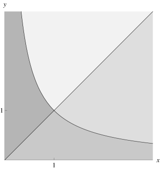
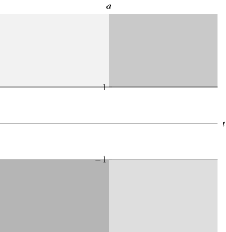
Figure 1: Projection of the domain $D$ onto the plane $(x,y)$. It is separated by the curves $x=y,\,xy=1$ into four parts marked by different colors, each mapped on the corresponding domain in Fig. 2.

Figure 2: Projection of the domain $G$ (3.10) onto the plane $(t,a)$. It is separated into four parts corresponding to four subdomains on Fig. 2.

The formulae (2.32) map domain $D$ onto disconnected domain $G$

$$G=\left\{(a,b,t):a\geq 1,\,b\geq 0\right\}\cup\left\{(a,b,t):a\leq-1,\,b\leq 0\right\}$$ (3.10)

that is illustrated in Fig. 2, 2. After a simple calculation one obtains

$$\mathrm{I}^{u,v}(A,B,C)=\frac{1}{2^{u+v-1}}\int_{G}\frac{\mathrm{d}a\,\mathrm{d}b\,\mathrm{d}t\;|b|^{u+v-1}|t|^{2(u+v)+d-1}\exp\left(A\,a\,t-B\,b+C\,b\,t^{-1}\right)}{|1+a|^{1-u}|1-a|^{1-v}\left[b^{2}+(1+b^{2})t^{2}+a^{2}\,t^{4}\right]^{u+v+\frac{d}{2}}}\,.$$ (3.11)

Since the integral (3.8) is rewritten in the form (3.11) it is straightforward to prove the symmetry (3.9) applying the integration variable change $(a,b,t)\to(a,b,t^{\prime})$ where $t^{\prime}=\frac{b}{at}$. It corresponds to the transposition $a\,t\rightleftarrows b\,t^{-1}$ in (3.11). Indeed the integrand in (3.11) transforms correctly and the integration domain $G$ is mapped onto itself.

Thus the Yang-Baxter relation (3.6) at $i=j=k=+$ is established. In a similar way the rest seven three-term relations (3.6) can be checked. To realize it we note that expressions (3.5) for $\mathcal{R}^{+}$ and $\mathcal{R}^{-}$ are almost identical. They can be obtained from each other reflecting the integration variable $x\to-x$. In other words $\mathcal{R}^{+}$ and $\mathcal{R}^{-}$ differ solely in integration contour. In the first case one integrates over positive semiaxis and in the second case over negative one. Consequently to check one of the three-term relations (3.6) we have to consider the integral (3.8) taken over appropriate reflected domain $D$. For example at $i=j=-,\,k=+$ we integrate over $x\leq 0,y\leq 0,z\geq 0$ in (3.8). When the variable change (2.32) is performed, it leads to the integral (3.11) with a certain integration domain that can be found in Fig.2. The symmetry (3.9) is established as before by means of the variable change $a\,t\rightleftarrows b\,t^{-1}$ in (3.11) which preserves the integration domain as one can easily see. Let us stress that algebraic manipulations needed to prove the three-term relations (3.6) are the same in all eight cases. The only difference is in the integration domains in (3.8) or (3.11).

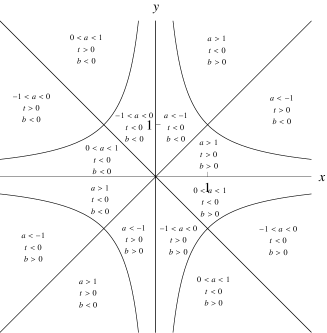
Figure 3: Projection of the domain $D$ and of its three reflections onto the plane $(x,y)$. Images of the subregions in the space $(a,b,t)$ are indicated (see (2.32)). It is assumed $z>0$. If otherwise $z<0$ then $b$ to be substituted on the figure by $-b$.

Finally, we have checked eight three-term relations (3.6) and hence we have proved the Yang-Baxter relation (1.11) for spinorial $\mathrm{R}$-matrix in fermionic realization. Using decomposition (3.4) of the $\mathrm{R}$-matrix in the sum of even and odd parts we obtain eight three-term

$$\mathrm{R}^{i}_{12}(u)\,\mathrm{R}^{k}_{23}(u+v)\,\mathrm{R}^{j}_{12}(v)=\mathrm{R}^{j}_{23}(v)\,\mathrm{R}^{k}_{12}(u+v)\,\mathrm{R}^{i}_{23}(u)\,$$ (3.12)

where $i,j,k=+,-$ (compare with (1.22)). However let us emphasize that we have always used above the fermionic representation for the $\mathrm{R}$-matrix.

At the end of Subsection 2.2 we have shown how to represent fermionic operators (2.13) in the matrix form (2.18). It can be easily checked that three-term relations (3.12) remain valid in both matrix representation $\rho^{\prime}$ and $\rho^{\prime\prime}$ (2.15). Thus the Yang-Baxter relation (1.11) for spinorial $\mathrm{R}$-matrix (1.9) is checked.

3.3 Unitarity relation

In the Introduction we have formulated unitarity relations (1.24) and proven them up to explicit calculation of coefficient functions $\mathrm{h}_{+}(u)$, $\mathrm{h}_{-}(u)$. Now we are going to fill this gap. We use fermionic realization of $\mathrm{R}$-matrix. In view of (2.13) and (2.28) one has

$$\mathrm{R}^{+}(u)\mathrm{R}^{+}(-u)=\mathrm{R}^{+}(u|x)\mathrm{R}^{+}(-u|y)\ast(1-xy)^{d}\mathrm{As}\left(e^{\frac{x+y}{1-xy}\,\Gamma_{1}\cdot\Gamma_{2}}\right)\,.$$ (3.13)

Since we know that $\mathrm{R}^{+}(u)\mathrm{R}^{+}(-u)$ is proportional to projector $\mathrm{P}^{+}$, formula (3.13) contains only fermionic structures $\mathbf{1}$ and $\mathrm{As}\left(\Gamma_{1}\cdot\Gamma_{2}\right)^{d}$. Coefficients at the other structures are equal to zero. Thus it will be sufficient for us to calculate numerical coefficient for $\mathbf{1}$ in (3.13) that is equal to

$$\textstyle{\mathrm{R}^{+}(u|x)\mathrm{R}^{+}(-u|y)\ast(1-xy)^{d}=\sum_{k=0}^{d/2}\binom{d}{2k}\mathrm{R}_{2k}(u)\mathrm{R}_{2k}(-u)\,.}$$

Similarly calculating numerical coefficient for $\mathrm{As}\left(\Gamma_{1}\cdot\Gamma_{2}\right)^{d}$ in (3.13) one obtains

$$\textstyle{\mathrm{R}^{+}(u|x)\mathrm{R}^{+}(-u|y)\ast(x+y)^{d}=\sum_{k=0}^{d/2}(-1)^{\frac{d}{2}}\binom{d}{2k}\mathrm{R}_{2k}(u)\mathrm{R}_{d-2k}(-u)\,.}$$

Further, using matrix representations $\rho^{\prime}$ (2.16) or $\rho^{\prime\prime}$ (2.17) one obtains (2.18)

$$\rho^{\prime}(\mathrm{R}^{+}(u))\rho^{\prime}(\mathrm{R}^{+}(-u))=\rho^{\prime\prime}(\mathrm{R}^{+}(u))\rho^{\prime\prime}(\mathrm{R}^{+}(-u))=\rho(\mathrm{R}^{+}(u))\rho(\mathrm{R}^{+}(-u))\,$$

that leads finally to the first unitarity relation (1.24) in view of (2.19).

The previous arguments are valid also for $\mathrm{R}^{-}(u)\mathrm{R}^{-}(-u)$. The coefficient function for $\mathbf{1}$ is equal to

$$\textstyle{\mathrm{R}^{-}(u|x)\mathrm{R}^{-}(-u|y)\ast(1-xy)^{d}=-\sum_{k=0}^{d/2-1}\binom{d}{2k+1}\mathrm{R}_{2k+1}(u)\mathrm{R}_{2k+1}(-u)\,.}$$

The matrix realization of the second unitarity relation (1.24) is provided by

$$\rho^{\prime}(\mathrm{R}^{-}(u))\rho^{\prime}(\mathrm{R}^{-}(-u))=\rho^{\prime\prime}(\mathrm{R}^{-}(u))\rho^{\prime\prime}(\mathrm{R}^{-}(-u))=-\rho(\mathrm{R}^{-}(u))\rho(\mathrm{R}^{-}(-u))\,.$$

Remark. Unitarity relations (1.24) can be established as well be means of integral representation for $\mathrm{R}$-matrix (3.1) using

$$\int\limits^{\infty}_{0}\int\limits^{\infty}_{0}\frac{\mathrm{d}x\,\mathrm{d}y\;x^{u-1}y^{-u-1}(x+y)^{k}(1-xy)^{d-k}}{(1+x^{2})^{u+\frac{d}{2}}(1+y^{2})^{-u+\frac{d}{2}}}=\left\{\begin{array}[]{ccl}-\frac{2\pi}{u}\frac{1}{\sin\pi u}\;,&\text{at}&\;k=0\\[5.69046pt] -\frac{2\pi}{u}\cot\pi u\;,&\text{at}&\;k=d\\[5.69046pt] 0\;,&\text{at}&\;k=1,\cdots,d-1\,.\end{array}\right.$$

Appendix A Appendix

In [1] we introduced representation space $V^{\prime}$ which we assumed to be infinite-dimensional in general and restricted the universal Yang-Baxter equation (1.1) to the space $V\otimes V\otimes V^{\prime}$

$$\mathrm{R}_{12}(u-v)\,\mathrm{L}_{13}(u)\,\mathrm{L}_{23}(v)=\mathrm{L}_{13}(v)\,\mathrm{L}_{23}(u)\,\mathrm{R}_{12}(u-v)\;\;\in\;\;{\rm End}(V\otimes V\otimes V^{\prime})\;.$$ (A.1)

The operator $\mathrm{L}(u)$ which is defined in the tensor product $V\otimes V^{\prime}$ of spinor and arbitrary representation $T^{\prime}$ spaces has been sought for in the form

$$\mathrm{L}(u)=u+\frac{i}{4}\,\gamma_{ab}\otimes T^{\prime}(M^{ab})\,.$$ (A.2)

Here notation (2.2) is used and $M_{ab}$ $(a,b=1,\dots,d)$ are generators of $so(d)$ subjected to relations

$$[M_{ab},M_{dc}]=i(\delta_{bd}M_{ac}+\delta_{ac}M_{bd}-\delta_{ad}M_{bc}-\delta_{bc}M_{ad})\,.$$ (A.3)

In [1] we claimed that $\mathrm{RLL}$-relation (A.1) with spinorial $\mathrm{R}$-matrix (1.9) is satisfied if representation $T^{\prime}$ is such that

$$T^{\prime}\left(\left\{M_{[ab}\,,M_{c]d}\right\}\right)=0\;,$$ (A.4)

where $\left\{A\,,B\right\}=A\,B+B\,A$ is anticommutator and square brackets denote antisymmetrization. We will undertake corresponding calculation in the first part of this Appendix using generating function technique. We are going to show that $\mathrm{RLL}$-relation (A.1) with $\mathrm{L}$-operator (A.2) and $\mathrm{R}$-matrix of the form (1.9) leads to recurrence relation (1.10) for coefficient functions $\mathrm{R}_{k}(u)$ and set up restriction (A.4) on the representation $T^{\prime}$ in the quantum space.

In order to avoid misunderstandings let us note that in a special case $d=6$ we have the isomorphism $so(6,\mathbb{C})=sl(4,\mathbb{C})$, corresponding $8$-dimensional $\mathrm{L}$-operator (A.2) is a direct sum of two $4$-dimensional $\mathrm{L}$-operators of $s\ell(4)$ algebra, spinorial $\mathrm{R}$-matrix (1.9) reduces to Yang $\mathrm{R}$-matrix under Weyl projections and condition (A.4) on representation $T^{\prime}$ happens to be superfluous. We demonstrate it in the second part of this Appendix.

A.1 $\mathrm{RLL}$-relation

Further by abuse of notation we denote $T^{\prime}(M_{ab})\rightarrow M_{ab}$. The following calculation is very similar to the one presented in Subsection 2.3, and it uses the generating function technique. We are going to prove fermionic version of $\mathrm{RLL}$-relation (A.1). Then taking matrix representation $\rho^{\prime}$ or $\rho^{\prime\prime}$ (2.15) one obtains immediately (A.1) for spinorial $\mathrm{R}$-matrix (1.9) and $\mathrm{L}$-operator (A.2).

The substitution of spinorial $\mathrm{R}$-matrix (2.13) in fermionic realization and fermionic analogue of $\mathrm{L}$-operator (A.2) with unspecified representation $T^{\prime}$ in the quantum space in $\mathrm{RLL}$-relation (A.1) gives

$$\sum_{k=0}^{\infty}\frac{\mathrm{R}_{k}(u-v)}{k!}\left(\Gamma_{1}\right)_{A_{k}}\left(\Gamma_{2}\right)^{A_{k}}\,\left(u+\frac{i}{4}\left(\Gamma_{1}\right)_{ab}M^{ab}\right)\left(v+\frac{i}{4}\left(\Gamma_{2}\right)_{cd}M^{cd}\right)=$$

$$=\sum_{k=0}^{\infty}\frac{\mathrm{R}_{k}(u-v)}{k!}\left(v+\frac{i}{4}\left(\Gamma_{1}\right)_{ab}M^{ab}\right)\left(u+\frac{i}{4}\left(\Gamma_{2}\right)_{cd}M^{cd}\right)\left(\Gamma_{1}\right)_{A_{k}}\left(\Gamma_{2}\right)^{A_{k}}\,.$$ (A.5)

This relation contains terms linear and quadratic in generators $M_{ab}$. The product of two generators can be transformed by means of Lie algebra commutation relations (A.3)

$$M_{ab}\,M_{cd}=\frac{1}{2}\,\left[M_{ab}\,,M_{cd}\right]+\frac{1}{2}\,\left\{M_{ab}\,,M_{cd}\right\}=\frac{i}{2}\,\left[g_{bc}M_{ad}-g_{ad}M_{cb}-g_{ac}M_{bd}+g_{bd}M_{ca}\right]+\frac{1}{2}\,\left\{M_{ab}\,,M_{cd}\right\}$$

so that

$$\left(\Gamma_{1}\right)_{ab}\left(\Gamma_{2}\right)_{cd}\,M^{ab}\,M^{cd}=-2i\left(\Gamma_{1}\right)_{a}^{\,\,\,c}\left(\Gamma_{2}\right)_{bc}\,M^{ab}+\frac{1}{2}\left(\Gamma_{1}\right)_{ab}\left(\Gamma_{2}\right)_{cd}\left\{M^{ab}\,,M^{cd}\right\}\,.$$

All terms in (A.5) linear on spectral parameters are combined in a single one $\sim(u-v)$ due to relation

$$\left(\Gamma_{1}\right)_{A_{k}}\left(\Gamma_{2}\right)^{A_{k}}\left(\Gamma_{2}\right)_{ab}-\left(\Gamma_{1}\right)_{ab}\left(\Gamma_{1}\right)_{A_{k}}\left(\Gamma_{2}\right)^{A_{k}}=\left(\Gamma_{1}\right)_{A_{k}}\left(\Gamma_{2}\right)_{ab}\left(\Gamma_{2}\right)^{A_{k}}-\left(\Gamma_{1}\right)_{A_{k}}\left(\Gamma_{1}\right)_{ab}\left(\Gamma_{2}\right)^{A_{K}}\,,$$

that is a consequence of the $so(d)$ invariance

$$\left[\,\left(\Gamma_{1}\right)_{ab}+\left(\Gamma_{2}\right)_{ab}\,,\left(\Gamma_{1}\right)_{A_{k}}\left(\Gamma_{2}\right)^{A_{k}}\,\right]=0\,.$$

After all intertwining relation (A.5) is reduced to the form

$$\sum_{k=0}^{\infty}\frac{\mathrm{R}_{k}(u)}{k!}\,u\,M^{ab}\,\biggl{(}\left(\Gamma_{1}\right)_{A_{k}}\left(\Gamma_{2}\right)^{A_{k}}\left(\Gamma_{2}\right)_{ab}-\left(\Gamma_{1}\right)_{ab}\left(\Gamma_{1}\right)_{A_{k}}\left(\Gamma_{2}\right)^{A_{k}}\biggl{)}+$$

$$+\frac{1}{2}\,\sum_{k=0}^{\infty}\frac{\mathrm{R}_{k}(u)}{k!}\,M^{ab}\,\biggl{(}\left(\Gamma_{1}\right)_{A_{k}}\left(\Gamma_{1}\right)_{a}^{\,\,\,c}\left(\Gamma_{2}\right)^{A_{k}}\left(\Gamma_{2}\right)_{bc}-\left(\Gamma_{1}\right)_{a}^{\,\,\,c}\left(\Gamma_{1}\right)_{A_{k}}\left(\Gamma_{2}\right)_{bc}\left(\Gamma_{2}\right)^{A_{k}}\biggl{)}+$$

$$+\frac{i}{8}\,\sum_{k=0}^{\infty}\frac{\mathrm{R}_{k}(u)}{k!}\,\biggl{(}\left(\Gamma_{1}\right)_{A_{k}}\left(\Gamma_{1}\right)_{ab}\left(\Gamma_{2}\right)^{A_{k}}\left(\Gamma_{2}\right)_{cd}-\left(\Gamma_{1}\right)_{cd}\left(\Gamma_{1}\right)_{A_{k}}\left(\Gamma_{2}\right)_{ab}\left(\Gamma_{2}\right)^{A_{k}}\biggl{)}\,\left\{M^{ab}\,,M^{cd}\right\}=0\,.$$ (A.6)

Using the reference formulae for products of generating functions (see (2.22))

$$\mathrm{As}\left(e^{x\Gamma_{1}\cdot\Gamma_{2}}\right)\,e^{s\cdot\Gamma_{1}}=\mathrm{As}\left(e^{x\Gamma_{1}\cdot\Gamma_{2}+s\cdot(\Gamma_{1}-x\Gamma_{2})}\right)\ \ ;\ \ e^{s\cdot\Gamma_{1}}\,\mathrm{As}\left(e^{x\Gamma_{1}\cdot\Gamma_{2}}\right)=\mathrm{As}\left(e^{x\Gamma_{1}\cdot\Gamma_{2}+s\cdot(\Gamma_{1}+x\Gamma_{2})}\right)\,,$$

$$\mathrm{As}\left(e^{x\Gamma_{1}\cdot\Gamma_{2}}\right)\,e^{t\cdot\Gamma_{2}}=\mathrm{As}\left(e^{x\Gamma_{1}\cdot\Gamma_{2}+t\cdot(\Gamma_{2}+x\Gamma_{1})}\right)\ \ ;\ \ e^{t\cdot\Gamma_{2}}\,\mathrm{As}\left(e^{x\Gamma_{1}\cdot\Gamma_{2}}\right)=\mathrm{As}\left(e^{x\Gamma_{1}\cdot\Gamma_{2}+t\cdot(\Gamma_{2}-x\Gamma_{1})}\right)\,,$$

it is easy to derive compact expression for the first term in (A.6)

$$\sum_{k=0}^{\infty}\frac{\mathrm{R}_{k}}{k!}M^{ab}\left[\left(\Gamma_{1}\right)_{A_{k}}\left(\Gamma_{2}\right)^{A_{k}}\left(\Gamma_{2}\right)_{ab}-\left(\Gamma_{1}\right)_{ab}\left(\Gamma_{1}\right)_{A_{k}}\left(\Gamma_{2}\right)^{A_{k}}\right]=$$

$$=\mathrm{R}(x)\ast M^{ab}\partial_{s_{a}}\partial_{s_{b}}\mathrm{As}\,e^{x\Gamma_{1}\cdot\Gamma_{2}}\left[e^{s\cdot(\Gamma_{2}+x\Gamma_{1})}-e^{s\cdot(\Gamma_{1}+x\Gamma_{2})}\right]=$$

$$=\mathrm{R}(x)\ast\,M^{ab}\,\mathrm{As}\,e^{x\Gamma_{1}\cdot\Gamma_{2}}\,\biggl{[}(\Gamma_{2a}+x\Gamma_{1b})(\Gamma_{2b}+x\Gamma_{1a})-(\Gamma_{1a}+x\Gamma_{2a})(\Gamma_{1b}+x\Gamma_{2b})\biggr{]}=$$

$$=\mathrm{R}(x)\ast\left(x^{2}-1\right)M^{ab}\mathrm{As}\,e^{x\Gamma_{1}\cdot\Gamma_{2}}\left[\Gamma_{1a}\Gamma_{1b}-\Gamma_{2a}\Gamma_{2b}\right]=\left(\partial^{2}_{x}\mathrm{R}(x)-\mathrm{R}(x)\right)\ast M^{ab}\mathrm{As}\,e^{x\Gamma_{1}\cdot\Gamma_{2}}\left[\Gamma_{1a}\Gamma_{1b}-\Gamma_{2a}\Gamma_{2b}\right]\,.$$

In a similar way using

$$\mathrm{As}\left(e^{x\Gamma_{1}\cdot\Gamma_{2}}\right)\,e^{s\cdot\Gamma_{1}+t\cdot\Gamma_{2}}=\mathrm{As}\left(e^{x(\Gamma_{1}-s)\cdot(\Gamma_{2}-t)+s\cdot\Gamma_{1}+t\cdot\Gamma_{2}}\right)\,,$$

$$e^{s\cdot\Gamma_{1}+t\cdot\Gamma_{2}}\,\mathrm{As}\left(e^{x\Gamma_{1}\cdot\Gamma_{2}}\right)=\mathrm{As}\left(e^{x(\Gamma_{1}+s)\cdot(\Gamma_{2}+t)+s\cdot\Gamma_{1}+t\cdot\Gamma_{2}}\right)\,,$$

the second term in (A.6) can be rearranged as follows

$$\sum_{k=0}^{\infty}\frac{\mathrm{R}_{k}}{k!}\,M^{ab}\,\left(\left(\Gamma_{1}\right)_{A_{k}}\left(\Gamma_{1}\right)_{a}^{\,\,\,c}\left(\Gamma_{2}\right)^{A_{k}}\left(\Gamma_{2}\right)_{bc}-\left(\Gamma_{1}\right)_{a}^{\,\,\,c}\left(\Gamma_{1}\right)_{A_{k}}\left(\Gamma_{2}\right)_{bc}\left(\Gamma_{2}\right)^{A_{k}}\right)=$$

$$=-2\,\mathrm{R}(x)\ast\,M^{ab}\,\,\mathrm{As}\,e^{x\Gamma_{1}\cdot\Gamma_{2}}\,\left[\Gamma_{1a}\Gamma_{1b}-\Gamma_{2a}\Gamma_{2b}\right]\biggl{[}(x^{3}+x)\,\Gamma_{1c}\Gamma_{2}^{c}-(d-2)\,x^{2}\biggl{]}=$$

$$=-2\biggl{[}x\,\partial^{3}_{x}\mathrm{R}(x)+x\,\partial_{x}\mathrm{R}(x)-(d-2)\,\partial^{2}_{x}\mathrm{R}(x)\biggl{]}\,M^{ab}\,\,\mathrm{As}\,e^{x\Gamma_{1}\cdot\Gamma_{2}}\,\left[\Gamma_{1a}\Gamma_{1b}-\Gamma_{2a}\Gamma_{2b}\right]\,,$$

and the last term in (A.6) takes the form

$$\sum_{k=0}^{\infty}\frac{\mathrm{R}_{k}}{k!}\,\biggl{(}\left(\Gamma_{1}\right)_{A_{k}}\left(\Gamma_{1}\right)_{ab}\left(\Gamma_{2}\right)^{A_{k}}\left(\Gamma_{2}\right)_{cd}-\left(\Gamma_{1}\right)_{cd}\left(\Gamma_{1}\right)_{A_{k}}\left(\Gamma_{2}\right)_{ab}\left(\Gamma_{2}\right)^{A_{k}}\biggl{)}\left\{M^{ab}\,,M^{cd}\right\}=$$

$$=4\,\mathrm{R}(x)\ast\,(x^{3}-x)\,\left\{M^{ab}\,,M^{cd}\right\}\mathrm{As}\,e^{x\Gamma_{1}\cdot\Gamma_{2}}\,\biggl{[}\Gamma_{1a}\Gamma_{1b}\Gamma_{1c}\Gamma_{2d}-\Gamma_{2a}\Gamma_{2b}\Gamma_{2c}\Gamma_{1d}\biggl{]}=$$

$$=4\,\biggl{[}\partial^{3}_{x}\mathrm{R}(x)-\partial_{x}\mathrm{R}(x)\biggl{]}\ast\,\left\{M^{ab}\,,M^{cd}\right\}\mathrm{As}\,e^{x\Gamma_{1}\cdot\Gamma_{2}}\,\biggl{[}\Gamma_{1a}\Gamma_{1b}\Gamma_{1c}\Gamma_{2d}-\Gamma_{2a}\Gamma_{2b}\Gamma_{2c}\Gamma_{1d}\biggl{]}\,.$$

Thus finally we obtain that (A.6) is equivalent to the relation

$$\biggl{[}x\,\partial^{3}_{x}\mathrm{R}(x)+x\,\partial_{x}\mathrm{R}(x)-(d-2)\,\partial^{2}_{x}\mathrm{R}(x)-u\left(\partial^{2}_{x}\mathrm{R}(x)-\mathrm{R}(x)\right)\biggl{]}\ast\,M^{ab}\,\,\mathrm{As}\,e^{x\Gamma_{1}\cdot\Gamma_{2}}\,\left[\Gamma_{1a}\Gamma_{1b}-\Gamma_{2a}\Gamma_{2b}\right]-$$

$$-\frac{i}{2}\,\biggl{[}\partial^{3}_{x}\mathrm{R}(x)-\partial_{x}\mathrm{R}(x)\biggl{]}\ast\,\left\{M^{ab}\,,M^{cd}\right\}\mathrm{As}\,e^{x\Gamma_{1}\cdot\Gamma_{2}}\,\biggl{[}\Gamma_{1a}\Gamma_{1b}\Gamma_{1c}\Gamma_{2d}-\Gamma_{2a}\Gamma_{2b}\Gamma_{2c}\Gamma_{1d}\biggl{]}=0\,.$$ (A.7)

There are two independent gamma-matrix structures in the latter formula so that the differential equation for the coefficient function $\mathrm{R}(x)$

$$x\biggl{[}\partial^{3}_{x}\mathrm{R}(x)+\partial_{x}\mathrm{R}(x)\biggl{]}-(d-2)\,\partial^{2}_{x}\mathrm{R}(x)-u\biggl{[}\partial^{2}_{x}\mathrm{R}^{\prime\prime}(x)-\mathrm{R}(x)\biggl{]}=0$$

and requirement $\left\{M_{[ab}\,,M_{c]d}\right\}=0$ (see (A.4)) arise. The differential equation produces the recurrence relation (see (1.10)) for the coefficients $\mathrm{R}_{k}(u)$:

$$\mathrm{R}(x)=\sum_{k=0}^{\infty}\frac{s_{k}\,\mathrm{R}_{k}(u)}{k!}\,x^{k}\ \longrightarrow\mathrm{R}_{k+2}(u)=-\frac{u+k}{u+d-2-k}\,\mathrm{R}_{k}(u)\,.$$

A.2 $\mathrm{R}$-matrix in the special case $d=6$

Now we proceed to the special case $d=6$. The recurrent relations (1.10) for odd and even coefficients are independent that enables us to fix $\mathrm{R}_{0}(u)=(u+4)/8$ and $\mathrm{R}_{1}(u)=0$. Hence $\mathrm{R}$-matrix (1.9) takes the form

$$\mathrm{R}(u)=\mathrm{R}_{0}(u)\,\mathbf{1}\otimes\mathbf{1}+\frac{\mathrm{R}_{2}(u)}{2!}\,\gamma_{a_{1}a_{2}}\otimes\gamma^{a_{1}a_{2}}+\frac{\mathrm{R}_{4}(u)}{4!}\,\gamma_{a_{1}\ldots a_{4}}\otimes\gamma^{a_{1}\ldots a_{4}}+\frac{\mathrm{R}_{6}(u)}{6!}\,\gamma_{a_{1}\ldots a_{6}}\otimes\gamma^{a_{1}\ldots a_{6}}$$ (A.8)

where

$$\mathrm{R}_{0}(u)=(u+4)/8\;,\;\mathrm{R}_{2}(u)=-u/8\;,\;\mathrm{R}_{4}(u)=u/8\;,\;\mathrm{R}_{6}(u)=-(u+4)/8$$

and the last term in (A.7) which is responsible for the condition (A.4) reduces to

$$\frac{2}{3!}\biggl{[}\mathrm{R}_{6}(u)+\mathrm{R}_{4}(u)\biggl{]}\,\left\{M^{ab}\,,M^{c}{}_{d}\right\}\,\biggl{[}\gamma_{abcc_{1}c_{2}c_{3}}\otimes\gamma^{dc_{1}c_{2}c_{3}}+\gamma^{dc_{1}c_{2}c_{3}}\otimes\gamma_{abcc_{1}c_{2}c_{3}}\biggl{]}\;.$$ (A.9)

All the other terms vanish because of the special form of coefficients $\mathrm{R}_{k}(u)$ and owing to finiteness of the Clifford algebra of gamma-matrices. Next we note that owing to $\alpha\,\gamma_{abcc_{1}c_{2}c_{3}}=\epsilon_{abcc_{1}c_{2}c_{3}}\,\gamma_{7}$ and $\gamma_{7}\gamma_{7}=\mathbf{1}$ (1.13) the gamma-matrix structure in (A.9) can be transformed as follows

$$\gamma_{abcc_{1}c_{2}c_{3}}\otimes\gamma^{dc_{1}c_{2}c_{3}}=\gamma_{7}\otimes\gamma_{7}\,\gamma_{abcc_{1}c_{2}c_{3}}\gamma^{dc_{1}c_{2}c_{3}}=120\,\gamma_{7}\otimes\gamma_{7}\left[\,\delta^{d}_{a}\,\gamma_{bc}-\delta^{d}_{b}\,\gamma_{ac}+\delta^{d}_{c}\,\gamma_{ab}\,\right]\;.$$

Consequently (A.9) which is proportional to

$$\left\{M^{ab}\,,M^{c}{}_{d}\right\}\left[\,\delta^{d}_{a}\,\gamma_{bc}-\delta^{d}_{b}\,\gamma_{ac}+\delta^{d}_{c}\,\gamma_{ab}\,\right]=2\left\{M^{a(b}\,,M^{c)}{}_{a}\right\}\,\gamma_{bc}=0$$

turns to zero. In the last expression the parentheses $(...)$ denote symmetrization. Therefore $\mathrm{RLL}$-equation (A.5) is valid for arbitrary representation of generators $\{M_{ab}\}$ of the algebra $so(6)$.

Let us rewrite the expression for $\mathrm{R}$-matrix (A.8) in a more transparent form. All gamma-matrix structures in (A.8) have block-diagonal form in Weyl representation for gamma-matrices. Therefore it is reasonable to consider projections of (A.8) on corresponding irreducible subspaces. We introduce subspaces $V_{+}$ and $V_{-}$ obtained by Weyl projections: $V_{+}=\frac{1+\Gamma_{7}}{2}V$ and $V_{-}=\frac{1-\Gamma_{7}}{2}V$. At first we note that relations

$$\left[\mathbf{1}\otimes\mathbf{1}-\frac{1}{6!}\,\gamma_{A_{6}}\otimes\gamma^{A_{6}}\right]_{V_{+}\otimes V_{-}}=\left[\frac{1}{2!}\,\gamma_{A_{2}}\otimes\gamma^{A_{2}}-\frac{1}{4!}\,\gamma_{A_{4}}\otimes\gamma^{A_{4}}\right]_{V_{+}\otimes V_{-}}=0\;$$

lead to $\left.\mathrm{R}(u)\right|_{V_{+}\otimes V_{-}}=\left.\mathrm{R}(u)\right|_{V_{-}\otimes V_{+}}=0$. Further a pair of relations

$$\left[\mathbf{1}\otimes\mathbf{1}+\frac{1}{6!}\,\gamma_{A_{6}}\otimes\gamma^{A_{6}}\right]_{V_{-}\otimes V_{-}}=\left[\frac{1}{2!}\,\gamma_{A_{2}}\otimes\gamma^{A_{2}}+\frac{1}{4!}\,\gamma_{A_{4}}\otimes\gamma^{A_{4}}\right]_{V_{-}\otimes V_{-}}=0$$

leads to Yang $\mathrm{R}$-matrix

$$\left.\mathrm{R}(u)\right|_{V_{-}\otimes V_{-}}=\left[2\;\mathrm{R}_{0}(u)\,\mathbf{1}\otimes\mathbf{1}+\mathrm{R}_{2}(u)\,\gamma_{ab}\otimes\gamma^{ab}\right]_{V_{-}\otimes V_{-}}={\bf 1}\otimes{\bf 1}+u\,\mathrm{P}\;$$

where $\mathrm{P}$ is a permutation operator and we take into account $\left.-\frac{1}{8}\,\gamma_{ab}\otimes\gamma^{ab}\right|_{V_{-}\otimes V_{-}}=\mathrm{P}-\frac{1}{4}\,{\bf 1}\otimes{\bf 1}\,.$ Analogously one concludes that $\left.\mathrm{R}(u)\right|_{V_{+}\otimes V_{+}}={\bf 1}\otimes{\bf 1}+u\,\mathrm{P}\;$.

References

• [1] D. Chicherin, S. Derkachov and A.P. Isaev,  Conformal group: R-matrix and star-triangle relation e-Print: arXiv:1206.4150 [math-ph]
• [2] R.Shankar and E.Witten, The $S$-matrix of the kinks of the $(\bar{\psi}\psi)^{2}$ model, Nucl.Phys. B141 (1978) 349-363.
• [3] A.B. Zamolodchikov and Al.B. Zamolodchikov, Factorized S-Matrices In Two Dimensions As The Exact Solutions Of Certain Relativistic Quantum Field Models, Ann. Phys. (N. Y.) 120 (1979) 253; Relativistic Factorized S Matrix In Two-Dimensions Having O(N) Isotopic Symmetry, Nucl. Phys. B 133 (1978) 525.
• [4] M.Karowski and H.J.Thun,  Complete S-matrix of the $O(2N)$ Gross-Neveu model, Nucl.Phys. B190[FS3] (1981) 61-92.
• [5] Al.B. Zamolodchikov, ”Factorizable Scattering in Assimptotically Free 2-dimensional Models of Quantum Field Theory”, PhD Thesis, Dubna (1979), unpublished.
• [6] N.Yu. Reshetikhin, Algebraic Bethe-Ansatz for $SO(N)$ invariant transfer-matrices, Zap. Nauch. Sem. LOMI, vol. 169 (1988) 122 (Journal of Math. Sciences, Vol.54, No. 3 (1991) 940-951).
• [7] A.N. Vasiliev, S.E. Derkachov and N.A. Kivel,  A Technique for calculating the gamma matrix structures of the diagrams of a total four fermion interaction with infinite number of vertices in $d=2+\epsilon$-dimensional regularization, Theor.Math.Phys. 103 (1995) 487-495, Teor.Mat.Fiz. 103 (1995) 179-191
• [8] A.N. Vasiliev, Functional methods in quantum field theory and statistics, London: Gordon-Breach, 1998.
• [9] A.N. Vasiliev, The field theoretic renormalization group in critical behavior theory and stochastic dynamics, Boca Raton: Chapman-Hall/CRC, 2004.
• [10] L.D. Faddeev and A.A. Slavnov, Gauge Fields. Introduction to quantum theory, (2nd edition). Addison-Wesley Publishing Company, 1991
• [11] J. Zinn-Justin, Quantum Field Theory and Critical Phenomena, (4th edition). Oxford University Press, Oxford, 2002
• [12] J.M. Maillet and F.W.Nijhoff, Integrability for multidimensional lattice models, Phys.Lett. B 224 (1989) 389-396; J.M. Maillet, Integrable systems and gauge theories, Nucl.Phys.(Proc.Suppl.) 18B (1990) 212-241.
• [13] R.M.Kashaev, On discrete Tree-Dimensional Equations Associated with the Local Yang-Baxter Relation, Lett.Math.Phys. 35 (1996) 389-397.
• [14] A.P. Isaev, Quantum groups and Yang-Baxter equations, Sov.J.Part.Nucl. 26 (1995) 501-526; (see also extended version: A.P. Isaev, Quantum groups and Yang-Baxter equations, preprint MPIM (Bonn), MPI 2004-132 (2004), http://www.mpim-bonn.mpg.de/html/preprints/preprints.html).