Time-Continuous Bell Measurements

Abstract

We combine the concept of Bell measurements, in which two systems are projected into a maximally entangled state, with the concept of continuous measurements, which concerns the evolution of a continuously monitored quantum system. For such time-continuous Bell measurements we derive the corresponding stochastic Schrödinger equations, as well as the unconditional feedback master equations. Our results apply to a wide range of physical systems, and are easily adapted to describe an arbitrary number of systems and measurements. Time-continuous Bell measurements therefore provide a versatile tool for the control of complex quantum systems and networks. As examples we show show that (i) two two-level systems can be deterministically entangled via homodyne detection, tolerating photon loss up to 50%, and (ii) a quantum state of light can be continuously teleported to a mechanical oscillator, which works under the same conditions as are required for optomechanical ground state cooling.

Introduction.— According to the basic rules of quantum mechanics a multipartite quantum system can be prepared in an entangled state by a strong projective measurement of joint properties of its subsystems. Measurements which project a system into a maximally entangled state are called Bell measurements and lie at the heart of fundamental quantum information processing protocols, such as quantum teleportation and entanglement swapping. In systems which are amenable to strong projective measurements (e. g., photons Bouwmeester et al. (1997); Sherson et al. (2006) and atoms Riebe et al. (2004); Barrett et al. (2004)), Bell measurements constitute a well established, versatile tool for quantum control and state engineering. However, in many physical systems only weak, indirect, but time-continuous measurements are available. Over the last years a multitude of experiments have demonstrated quantum-limited time-continuous measurement and control in a range of physical systems, including single atoms Bushev et al. (2006); Kubanek et al. (2009); Koch et al. (2010), cavity modes Sayrin et al. (2011); Haroche and Raimond (2006), atomic ensembles Smith et al. (2006); Chaudhury et al. (2007); Krauter et al. (2011), superconducting qubits Vijay et al. (2012); Ristè et al. (2013), and massive mechanical oscillators Arcizet et al. (2006); Corbitt et al. (2007); Mow-Lowry et al. (2008); Abbott et al. (2009). Continuously monitored quantum dynamics are described through the formalism of stochastic Schrödinger and master equations Belavkin (1980); Hudson and Parthasarathy (1984); Gardiner and Collett (1985); Gardiner et al. (1992); Wiseman and Milburn (1993a); Wiseman (1994); Doherty et al. (2000); Hopkins et al. (2003); Jacobs and Steck (2006); Bouten et al. (2007); Parthasarathy (1992); Carmichael (1993); Gardiner and Zoller (2004); Wiseman and Milburn (2009); Barchielli and Gregoratti (2009), which in itself constitutes a cornerstone of quantum control. Surprisingly, no exhaustive connection between these important concepts—Bell measurements and time-continuous measurements—has been made so far.

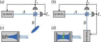
Figure 1: Schematic setups for (a) time-continuous teleportation and (b) entanglement swapping. The systems may take the form of (c) a harmonic oscillator (e. g., an optomechanical cavity), or (d) a two-level system (e. g., a single spin).

In this letter we establish this connection and introduce the notion of time-continuous Bell measurements , which are realized via continuous homodyne detection of electromagnetic fields, and can be applied to a great number of systems, including those which cannot be measured projectively. We derive the constitutive equations of motion—the conditional stochastic Schrödinger/master equation and the unconditional feedback master equation—of the monitored systems. In particular we study two generic scenarios: Time-continuous quantum teleportation of a general optical state of Gaussian (squeezed) white noise to a second system realizes a continuous remote state-preparation protocol [Fig. 1(a)]. Continuous entanglement swapping provides a means for dissipatively generating stationary entanglement [Fig. 1(b)]. The corresponding fundamental equations of motion are applicable to any of the above mentioned platforms Bushev et al. (2006); Kubanek et al. (2009); Koch et al. (2010); Sayrin et al. (2011); Haroche and Raimond (2006); Smith et al. (2006); Chaudhury et al. (2007); Krauter et al. (2011); Arcizet et al. (2006); Corbitt et al. (2007); Mow-Lowry et al. (2008); Abbott et al. (2009); Vijay et al. (2012); Ristè et al. (2013) and are the main result of this work. Along the lines of the present derivation, it is straightforward to treat different protocols, and to generalize our results to more complex setups involving an arbitrary number of systems and measurements, with applications in the continuous control of quantum networks.

To illustrate the power of our approach we demonstrate that two two-level systems can be continuously and deterministically driven to an entangled state—ideally a Bell state—through homodyne detection of light, tolerating photon losses up to 50%. This scheme can provide the basis for a dissipative quantum repeater architecture Vollbrecht et al. (2011). Furthermore we show how to implement time-continuous teleportation in an optomechanical system Chen (2013); Aspelmeyer et al. (2013) where the quantum state of continuous-wave light is continuously transferred to a moving mirror, requiring only an optomechanical cooperativity larger than one, as demonstrated in Murch et al. (2008); Teufel et al. (2011); Chan et al. (2011); Brooks et al. (2012); Purdy et al. (2013); Safavi-Naeini et al. (2013).

Continuous Teleportation.— We consider the setup shown in Fig. 1(a): A system $S$ couples to a 1D electromagnetic field $A$ via a linear interaction $H_{\mathrm{int}}=\mathrm{i}[s\,a^{\dagger}(t)-s^{\dagger}a(t)]$, where $s$ is a system operator (e. g. a cavity creation/destruction, or spin operator), and the light field is described (in an interaction picture at a central frequency $\omega_{0}$) by $a(t)=\int\mathrm{d}\omega\,a(\omega)\,\mathrm{e}^{-\mathrm{i}(\omega-\omega_{0})t}$. Analogously a second 1D field $B$ is described by an operator $b(t)$. Our first goal is to derive a stochastic master equation (SME) for the state of the system $S$, conditioned on the results of a time-continuous Bell measurement on the two fields $A$ and $B$. In a Markov approximation we restrict ourselves to white-noise fields, which means that both $a(t)$ and $b(t)$ are $\delta$-correlated. This allows us to introduce the Itō increment $\mathrm{d}A(t)=a(t)\mathrm{d}t$ (and analogously $\mathrm{d}A^{\dagger}$, $\mathrm{d}B$, $\mathrm{d}B^{\dagger}$), and to express the time evolution of the state $|\phi\rangle$ of the overall system ($S+A+B$) as a stochastic Schrödinger equation in Itō form Gardiner and Zoller (2004); Wiseman and Milburn (2009),

$$\mathrm{d}|\phi\rangle=\left(-\mathrm{i}H_{\mathrm{eff}}\mathrm{d}t+s\,\mathrm{d}A^{\dagger}\right)|\phi\rangle,$$ (1)

where $H_{\mathrm{eff}}=H_{\mathrm{sys}}-\mathrm{i}\frac{1}{2}s^{\dagger}s$, with the (unspecified) system Hamiltonian $H_{\mathrm{sys}}$.

We assume that the initial state of the overall system is $|\phi(0)\rangle=|\psi(0)\rangle_{S}|\mathrm{vac}\rangle_{A}|M\rangle_{B}$, where $|M\rangle$ is an arbitrary pure Gaussian state defined by the eigenvalue equation $[(N+M^{*}+1)b(t)-(N+M)b^{\dagger}(t)]|M\rangle_{B}=0$. The parameters $N\in\mathbb{R}$, $M\in\mathbb{C}$ obey the relations $N\geq 0$ ($N=M=0$ true for vacuum) and $|M|^{2}=N(N+1)$. The white noise model essentially assumes that the squeezing bandwidth is larger than all other system time scales. Making use of the fact that $a(t)|\phi(t)\rangle=a(t)|\phi(0)\rangle=0$ and the above eigenvalue equation, we can rewrite equation (1) in terms of the Einstein–Podolsky–Rosen EPR operators $X_{+}=(a+a^{\dagger}+b+b^{\dagger})/\sqrt{2}$ and $P_{-}=+\mathrm{i}(a-a^{\dagger}-b+b^{\dagger})/\sqrt{2}$, which can be simultaneously measured in this setup. The resulting equation reads

$$\mathrm{d}|\phi\rangle=\left[-\mathrm{i}H_{\mathrm{eff}}\mathrm{d}t+\,s\,(\mu\,\mathrm{d}X_{+}+\mathrm{i}\nu\,\mathrm{d}P_{-})\right]|\phi\rangle,$$ (2)

with $\mu=(1-M+M^{*})/(1+N+M^{*})$ and $\nu=\mathrm{i}(1+2N+M+M^{*})/(1+N+M^{*})$. Writing Eq. (1) in this form enables us to project (2) onto the EPR state $|I_{+}I_{-}\rangle_{AB}$, defined by $X_{+}|I_{+}I_{-}\rangle_{AB}=I_{+}|I_{+}I_{-}\rangle_{AB}$ and $P_{-}|I_{+}I_{-}\rangle_{AB}=I_{-}|I_{+}I_{-}\rangle_{AB}$. This leads to the so-called linear stochastic Schrödinger equation Carmichael (1993)

$$\mathrm{d}|\tilde{\psi}_{\mathrm{c}}\rangle=\left\{-\mathrm{i}H_{\mathrm{eff}}\mathrm{d}t+\,s\,[\mu I_{+}(t)+\mathrm{i}\nu I_{-}(t)]\mathrm{d}t\right\}|\tilde{\psi}_{\mathrm{c}}\rangle,$$ (3)

for the unnormalized system state $|\tilde{\psi}_{\mathrm{c}}\rangle$, which is conditioned on the measurement results $I_{\pm}$. Note that $I_{+}$ and $I_{-}$ are real-valued, Gaussian random processes, which are proportional to the measured homodyne photocurrents. As $I_{\pm}$ result from mixing the fields $A$ and $B$ on a beam-splitter, they carry information about both fields, and will therefore be correlated, which is a crucial feature of a Bell measurement. We can write Goetsch and Graham (1994); Wiseman and Milburn (2009)

$$I_{+}(t) =\sqrt{1/2}\langle s+s^{\dagger}\rangle_{\psi(t)}+\xi_{+}(t),$$ (4a)

$$I_{-}(t) =\mathrm{i}\sqrt{1/2}\langle s-s^{\dagger}\rangle_{\psi(t)}+\xi_{-}(t),$$ (4b)

where $\xi_{\pm}(t)=\mathrm{d}W_{\pm}(t)/\mathrm{d}t$ is zero-mean, Gaussian, white noise with corresponding Wiener increments $\mathrm{d}W_{\pm}$ Gardiner and Zoller (2004). The (co-)variances of $\mathrm{d}W_{\pm}$ are given by

$$w_{1}\,\mathrm{d}t {:=}(\mathrm{d}W_{+})^{2}=[N+1+(M+M^{*})/2]\mathrm{d}t,$$ (5a)

$$w_{2}\,\mathrm{d}t {:=}(\mathrm{d}W_{-})^{2}=[N+1-(M+M^{*})/2]\mathrm{d}t,$$ (5b)

$$w_{3}\,\mathrm{d}t {:=}\mathrm{d}W_{+}\mathrm{d}W_{-}=-[\mathrm{i}(M-M^{*})/2]\mathrm{d}t,$$ (5c)

as follows essentially from the initial mean values with respect to the optical fields $\langle(X_{+})^{2}\rangle_{\phi(0)}$, $\langle(P_{-})^{2}\rangle_{\phi(0)}$, etc. As expected, we in general find non-zero cross-correlations between $I_{+}$ and $I_{-}$, which depend on the squeezing properties of the input field $B$. Using Itō rules Gardiner and Zoller (2004) we can construct the corresponding stochastic master equation (in Itō form) for the system state conditioned on the Bell measurement result,

$$\mathrm{d}\rho_{\mathrm{c}}=\mathcal{L}\rho_{\mathrm{c}}\mathrm{d}t+\!\frac{1}{\sqrt{2}}\!\left\{\mathcal{H}[\mu s]\rho_{\mathrm{c}}\,\mathrm{d}W_{+}\!+\mathcal{H}[\mathrm{i}\nu s]\rho_{\mathrm{c}}\,\mathrm{d}W_{-}\right\},$$ (6)

where we defined $\mathcal{L}\rho=-\mathrm{i}[H_{\mathrm{sys}},\rho]+\mathcal{D}[s]\rho$, the Lindblad operator $\mathcal{D}[s]\rho=\left(s\rho s^{\dagger}-\frac{1}{2}\rho s^{\dagger}s-\frac{1}{2}s^{\dagger}s\rho\right)$, and $\mathcal{H}[s]\rho=\left(s-\langle s\rangle\right)\rho+\rho\left(s-\langle s\rangle\right)^{\dagger}$.

We now apply Hamiltonian feedback proportional to the homodyne photocurrents to the system, a scenario which covers the case of continuous quantum teleportation of the state of field $B$ to the system $S$. We follow Wiseman and Milburn (1993b) in order to derive the corresponding unconditional feedback master equation. Hamiltonian feedback is described by a term $[\dot{\rho}_{\mathrm{c}}]_{\mathrm{fb}}=\sqrt{1/2}\left(I_{+}\mathcal{K}_{+}+I_{-}\mathcal{K}_{-}\right)\rho_{\mathrm{c}}$, where we define $\mathcal{K}_{\pm}\rho=-\mathrm{i}[F_{\pm},\rho]$, and Hermitian operators $F_{\pm}$. After incorporating this feedback term into the SME (6), and taking the classical average over all possible measurement outcomes, $\rho=E[\rho_{c}]$, we arrive at the unconditional feedback master equation

$$\dot{\rho}=-\mathrm{i}\left[H_{\mathrm{sys}}+(1/4)\left\{(F_{+}+\mathrm{i}F_{-})s+s^{\dagger}(F_{+}-\mathrm{i}F_{-})\right\},\rho\right]\\ +(1/2)\big{\{}\mathcal{D}[s-\mathrm{i}F_{+}]\rho+\mathcal{D}[s-F_{-}]\rho+w_{3}\mathcal{D}[F_{+}+F_{-}]\rho\\ +(w_{1}-w_{3}-1)\mathcal{D}[F_{+}]\rho+(w_{2}-w_{3}-1)\mathcal{D}[F_{-}]\rho\big{\}}.$$ (7)

This is the main result of this section. The evolution of the system $S$ thus effectively depends on the state of the field $B$ (via $w_{i}$) which has never interacted with $S$, and which can in principle even change (adiabatically) in time. Eq. (7) can thus be viewed as a continuous “remote preparation” of quantum states.

To illustrate this point we consider the case where the target system $S$ is a bosonic mode. For a system to be amenable to continuous teleportation the system–field interaction must enable entanglement creation. We thus set $s=c^{\dagger}$, with $c$ a bosonic annihilation operator, and therefore obtain $H_{\mathrm{int}}\propto c\,a(t)+c^{\dagger}a^{\dagger}(t)$ (commonly known as two-mode-squeezing interaction). Additionally we choose $F_{+}=\mathrm{i}(c-c^{\dagger})$ and $F_{-}=(c+c^{\dagger})$, which means that the photocurrents $I_{+}$, $I_{-}$ will be fed-back to the $x$ and $p$ quadrature, respectively. The resulting equation can be brought into the form

$$\dot{\rho}=-\mathrm{i}[H_{\mathrm{sys}},\rho]+(2N+1)\mathcal{D}[J]\rho,$$ (8)

where the jump operator $J$ is determined by $J\propto-\mathrm{i}(2N+1-M-M^{*})x+(1+M-M^{*})p$ (with an appropriate normalization). For $H_{\mathrm{sys}}=0$ equation (8) has the steady-state solution $\rho_{\mathrm{ss}}=|\psi\rangle\langle\psi|$, where $J|\psi\rangle=0$. Up to a trivial transformation this state is identical to the input state $|M\rangle\langle M|$. Note that for the vacuum case $N=M=0$ we find $J=c$, which means that, devoid of other decoherence terms, the system will be driven to its ground state. Below, we will come back to this scenario, and discuss its implementation on the basis of an optomechanical system in more detail. First, however, we consider continuous entanglement swapping [Fig. 1(b)].

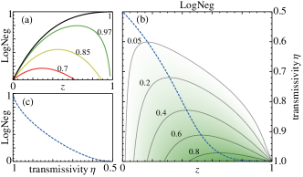
Figure 2: (Color online) Performance of continuous entanglement swapping: (a) Entanglement (logarithmic negativity Vidal and Werner (2002)) of the stationary state versus $z$ parameterizing the light-matter interaction $\propto\mathrm{i}[(\sqrt{z(1+z)}\sigma^{+}-\sqrt{1-z}\sigma^{-})a^{\dagger}(t)-\mathrm{h.c.}]$, with transmissivity $\eta$ as indicated. (b) Entanglement versus $z$ and $\eta$ for optimized gains. (c) Entanglement versus transmissivity for optimized $z$. Nonzero entanglement can be achieved even for losses approaching 50%.

Continuous Entanglement Swapping.— We now replace the Gaussian input state in mode $B$ with a field state emitted by a second system, which couples to the field $B$ via $H_{\mathrm{int}}=\mathrm{i}[s_{2}b^{\dagger}(t)-s_{2}^{\dagger}b(t)]$. Using the same logic as before we can derive the linear stochastic Schrödinger equation for the bipartite state $|\tilde{\psi}\rangle$ (of $S_{1}$ and $S_{2}$)

$$\mathrm{d}|\tilde{\psi}\rangle=\left[-\mathrm{i}H_{\mathrm{eff}}\mathrm{d}t+s_{+}I_{+}(t)\mathrm{d}t+\mathrm{i}s_{-}I_{-}(t)\mathrm{d}t\right]|\tilde{\psi}\rangle,$$ (9)

where now $H_{\mathrm{eff}}=H_{\mathrm{sys}}^{\mathrm{(1)}}+H_{\mathrm{sys}}^{\mathrm{(2)}}-\frac{\mathrm{i}}{2}\sum_{i=1,2}s_{i}^{\dagger}s_{i}$ and $s_{\pm}=s_{1}\pm s_{2}$. Accordingly, the homodyne currents read

$$I_{+}(t) =\sqrt{1/2}\,\langle s_{+}+s_{+}^{\dagger}\rangle_{\psi(t)}+\xi_{+}(t),$$ (10a)

$$I_{-}(t) =\mathrm{i}\sqrt{1/2}\,\langle s_{-}-s_{-}^{\dagger}\rangle_{\psi(t)}+\xi_{-}(t),$$ (10b)

and the corresponding SME is

$$\mathrm{d}\rho_{\mathrm{c}}=\mathcal{L}\rho_{\mathrm{c}}\mathrm{d}t+\sqrt{1/2}\left\{\mathcal{H}[s_{+}]\rho_{\mathrm{c}}\,\mathrm{d}W_{+}+\mathcal{H}[\mathrm{i}s_{-}]\rho_{\mathrm{c}}\,\mathrm{d}W_{-}\right\},$$ (11)

with $\mathcal{L}\rho=-\mathrm{i}[H^{\mathrm{(1)}}_{\mathrm{sys}}+H^{\mathrm{(2)}}_{\mathrm{sys}},\rho]+\mathcal{D}[s_{1}]\rho+\mathcal{D}[s_{2}]\rho$. Here, the Wiener increments are uncorrelated and have unit variance, i. e., $(\mathrm{d}W_{+})^{2}=(\mathrm{d}W_{-})^{2}=\mathrm{d}t$, $\mathrm{d}W_{+}\mathrm{d}W_{-}=0$. Applying feedback to either or both of the two systems in the same way as before gives rise to

$$\dot{\rho}=-\mathrm{i}\left[H,\rho\right]-\mathrm{i}(1/4)\left[(F_{+}s_{+}+\mathrm{i}F_{-}s_{-})+\mathrm{h.c.},\rho\right]\\ +(1/2)\mathcal{D}[s_{+}-\mathrm{i}F_{+}]\rho+(1/2)\mathcal{D}[s_{-}-F_{-}]\rho.$$ (12)

This is the desired feedback master equation for continuous entanglement swapping. For two bosonic modes with $s_{i}=c_{i}^{\dagger}$, applying a feedback strategy analogous to the case of teleportation above will drive the two systems to an Einstein–Podolsky–Rosen entangled stationary state. In view of Fig. 1(b) the resulting topology comes close to a Michelson interferometer, for which a similar scheme was discussed in Müller-Ebhardt et al. (2008). Note, however, that the central equations (6), (7) and (9), (12) are general and also apply to non-Gaussian systems. As a rather surprising application we will show, that a pure entangled state of two two-level systems (TLS) can be created deterministically.

Consider two TLS which couple to 1D fields via operators $s_{1}=\sqrt{z(1+z)}\sigma_{1}^{+}+\sqrt{1-z}\sigma_{1}^{-}$ and $s_{2}=\sqrt{z(1+z)}\sigma_{2}^{+}-\sqrt{1-z}\sigma_{2}^{-}$ ($z\in[0,1]$). (For how to achieve this coupling see appendix D.) The fields are subject to a continuous Bell measurement as depicted in Fig. 1(b). The homodyne photocurrents $I_{\pm}(t)$ are used in a Hamiltonian feedback scheme to generate rotations of the TLS about their $x$ and $y$ axes according to $F_{+}=G_{-}\sigma^{y}_{1}+G_{+}\sigma^{y}_{2}$ and $F_{-}=G_{+}\sigma^{x}_{1}-G_{-}\sigma^{x}_{2}$, with gain coefficients $G_{\pm}=\sqrt{z/(1+z)}\left(1\pm\sqrt{z(1+z)/(1-z)}\right)$. For this choice of $s_{i}$ and $F_{\pm}$, and assuming that the levels in each TLS are degenerate (i. e., $H_{\mathrm{sys}}^{\mathrm{(}i\mathrm{)}}=0$), the jump operators in Eq. (12), become $J_{+}=s_{+}-\mathrm{i}F_{+}\propto j_{1}-\lambda j_{2}$ and $J_{-}=s_{-}-F_{-}\propto j_{2}+\lambda j_{1}$, where $j_{1}=\sigma_{1}^{-}+z\sigma_{2}^{+}$ and $j_{2}=\sigma_{2}^{-}+z\sigma_{1}^{+}$, and $\lambda$ is a real coefficient. The common dark state of the jump operators $J_{\pm}|\Phi\rangle=j_{1,2}|\Phi\rangle=0$ is the pure entangled state $|\Phi\rangle\propto|00\rangle-z|11\rangle$ which becomes a maximally entangled Bell state for $z\rightarrow 1$ Vollbrecht et al. (2011). The particular linear combination of $j_{1,2}$ in $J_{\pm}$ is chosen such, that the state $|\Phi\rangle$ is also an eigenstate of the effective Hamiltonian $\bar{H}_{\mathrm{eff}}=\tfrac{1}{4}[(F_{+}+\mathrm{i}F_{-})s_{1}+(F_{+}-\mathrm{i}F_{-})s_{2}+\mathrm{h.c.}]-\tfrac{\mathrm{i}}{4}[J_{+}^{\dagger}J_{+}+J_{-}^{\dagger}J_{-}]$ of Eq. (12), i. e., $\bar{H}_{\mathrm{eff}}|\Phi\rangle=0$. Together, these properties guarantee that the stationary state of Eq. (12) is the pure entangled state $|\Phi\rangle$ Kraus et al. (2008). Note that in this way entanglement is generated deterministically, in contrast to conditional schemes based on photon counting Bose et al. (1999); Duan and Kimble (2003); Simon and Irvine (2003); Browne et al. (2003); Campbell and Benjamin (2008); Vollbrecht and Cirac (2009); Santos et al. (2012). Also, it neither requires to couple nonclassical light into cavities Cirac et al. (1997); Pellizzari (1997); van Enk et al. (1997); Parkins and Kimble (2000); Mancini and Bose (2001); Clark et al. (2003); Kraus and Cirac (2004); Mancini and Bose (2004), or a parity measurement on two qubits Ristè et al. (2013). The necessary strong coupling of TLS to a 1D optical field can be achieved in a variety of physical systems, such as cavities Raimond et al. (2001); Miller et al. (2005); Walther et al. (2006); Haroche and Raimond (2006); Girvin et al. (2009); Vetsch et al. (2010); Goban et al. (2012) or atomic ensembles Hammerer et al. (2010); Saffman et al. (2010); Krauter et al. (2011).

The ideal limit of Bell state entanglement ($z\rightarrow 1$ ) is achieved only in the limit of infinite feedback gains $G_{\pm}$, as is to be expected for the present treatment. More sophisticated descriptions of feedback might relieve this restriction Wiseman and Milburn (2009). However, in the relevant case including losses, the optimal feedback gains stay finite even in the present description. Assuming that all passive photon losses, such as finite transmission and detector efficiency, are combined in one transmissivity (or efficiency) parameter $\eta$, we have to apply the generalized feedback master equation from appendix B instead of Eq. (12). For given $\eta$ and light matter interaction, i. e. fixed $z$, we optimize the feedback gains $G_{\pm}$ in order to maximize the entanglement of the stationary state $\rho_{\mathrm{ss}}$. We keep the particular form of the feedback Hamiltonians $F_{\pm}$ as it preserves the Bell diagonal structure of $\rho_{\mathrm{ss}}$. Fig. 2 shows that entanglement can be achieved even for losses approaching 50%, which is where the quantum capacity of the lossy bosonic channel drops to zero Wolf et al. (2007).

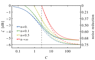
Figure 3: (Color online) Mechanical squeezing $\zeta$ against cooperativity $C$ for varying mechanical bath occupation $\bar{n}=0,1/10,1/2,\infty$ (represented by different colors/gray levels) and sideband resolution $\kappa/\omega_{\mathrm{m}}=1\ (10)$ [solid (dashed) lines]. The solid black line at $\zeta=-6\,\mathrm{dB}$ shows the squeezing level of the input light (corresponding to $N\approx 0.56$). The dashed vertical line shows the value of $C_{\mathrm{crit}}=1/[\sqrt{N(N+1)}-N]\approx 2.7$ above which mechanical squeezing is achievable for any $\bar{n}$.

Application to optomechanical systems.— In the remainder of this article we will show how continuous quantum teleportation can be implemented in an optomechanical system in the form of a Fabry–Pérot cavity with one oscillating mirror [Fig. 1(c)] Chen (2013); Aspelmeyer et al. (2013). Here the system Hamiltonian (in the laser frame at $\omega_{0}$) is $H_{\mathrm{sys}}=H_{0}+H_{\mathrm{om}}=(\omega_{\mathrm{m}}c_{\mathrm{m}}^{\dagger}c_{\mathrm{m}}+\Delta_{\mathrm{c}}c_{\mathrm{c}}^{\dagger}c_{\mathrm{c}})+g(c_{\mathrm{m}}+c_{\mathrm{m}}^{\dagger})(c_{\mathrm{c}}+c_{\mathrm{c}}^{\dagger})$, where $\omega_{\mathrm{m}}$ is the mechanical frequency, $\Delta_{\mathrm{c}}=\omega_{\mathrm{c}}-\omega_{0}$ is the detuning of the driving laser (at $\omega_{0}$) with respect to the cavity (at $\omega_{\mathrm{c}}$), and $g$ is the optomechanical coupling strength. $c_{\mathrm{m}}$ and $c_{\mathrm{c}}$ are bosonic annihilation operators of the mechanical and the optical mode respectively. We assume a cavity linewidth $\kappa$, a width of the mechanical resonance $\gamma$, and a mean phonon number $\bar{n}$ in thermal equilibrium.

In this system the ideal limit of continuous teleportation as given by Eq. (8) can be approached in the regime $g\ll\kappa\ll\omega_{\mathrm{m}}$ and for $\Delta_{\mathrm{c}}=-\omega_{\mathrm{m}}$, where the resonant terms in the optomechanical interaction are $H_{\mathrm{om}}=g(c_{\mathrm{m}}c_{\mathrm{c}}+c_{\mathrm{m}}^{\dagger}c_{\mathrm{c}}^{\dagger})$. Under the weak-coupling condition ($g\ll\kappa$) the cavity follows the mechanical mode adiabatically, and we effectively obtain the required entangling interaction between the mirror and the outgoing field. The mechanical oscillator resonantly scatters photons into the lower sideband such that photons which are correlated with the mechanical motion are spectrally located at $\omega_{0}-\omega_{\mathrm{m}}=\omega_{\mathrm{c}}$. Consequently, we have to modify the previous measurement setup in two ways: Firstly, we choose the center frequency of the squeezed input light at the same frequency $\omega_{\mathrm{c}}$. Secondly, we now use heterodyne detection to measure quadratures on the same sideband. These two modifications, together with the adiabatic elimination of the cavity (a perturbative expansion in $g/\kappa$ Doherty and Jacobs (1999)) and a rotating-wave approximation (an effective coarse-graining in time Gardiner and Zoller (2004)), allow us to write the SME for the mechanical system, in the rotating frame at $\omega_{\mathrm{m}}$, as

$$\mathrm{d}\rho_{\mathrm{c}}=\gamma_{-}\mathcal{D}[c_{\mathrm{m}}]{\rho}_{\mathrm{c}}\mathrm{d}t+\gamma_{+}\mathcal{D}[c_{\mathrm{m}}^{\dagger}]{\rho}_{\mathrm{c}}\mathrm{d}t\\ +\sqrt{g^{2}\kappa/2}\left\{\mathcal{H}[-\mathrm{i}\mu\eta_{+}c_{\mathrm{m}}^{\dagger}]{\rho}_{\mathrm{c}}\mathrm{d}W_{+}+\mathcal{H}[\nu\eta_{+}c_{\mathrm{m}}^{\dagger}]{\rho}_{\mathrm{c}}\mathrm{d}W_{-}\right\},$$ (13)

where $\eta_{\pm}=[\kappa/2+\mathrm{i}(\Delta_{\mathrm{c}}\pm\omega_{\mathrm{m}})]^{-1}$. The first two terms describe passive cooling and heating effects via the optomechanical interaction with cooling and heating rates $\gamma_{-}=\gamma(\bar{n}+1)+2g^{2}\mathrm{Re}(\eta_{-})$ and $\gamma_{+}=\gamma\bar{n}+2g^{2}\mathrm{Re}(\eta_{+})$, as was derived before in the quantum theory of optomechanical sideband cooling Wilson-Rae et al. (2007); Marquardt et al. (2007). The last two terms in (13) describe the continuous measurement in the sideband resolved regime for arbitrary laser detuning $\Delta_{\mathrm{c}}$. This is an extension of the conditional master equation for optomechanical systems usually considered in the literature which concerns a resonant drive and the bad-cavity limit Belavkin (1999); Hopkins et al. (2003) (see however Demchenko and Vyatchanin (2013)).

For simplicity we assume here that we can apply feedback directly to the mechanical oscillator. We can thus adopt the same choice of $F_{\pm}$ as before, and arrive at a feedback master equation similar to (8), $\dot{{\rho}}=\gamma(\bar{n}+1)\mathcal{D}[c_{\mathrm{m}}]{\rho}+\gamma\bar{n}\mathcal{D}[c_{\mathrm{m}}^{\dagger}]{\rho}+(4g^{2}/\kappa)\{\lambda_{1}(\epsilon)\mathcal{D}[J_{1}(\epsilon)]+\lambda_{2}(\epsilon)\mathcal{D}[J_{2}(\epsilon)]\}{\rho},$ where $\epsilon=[1+(4\omega_{\mathrm{m}}/\kappa)^{2}]^{-1}$. (For details on how to derive $\lambda_{i}$ and $J_{i}$ refer to appendix C) The protocol’s performance is degraded by mechanical decoherence effects and counter-rotating terms of the optomechanical coupling, which are suppressed by $\epsilon$. For fixed input squeezing (determined by $N$) the state of the mechanical oscillator is determined by $\bar{n}$, the sideband resolution $\kappa/\omega_{\mathrm{m}}$, and the cooperativity parameter $C=g^{2}/(\bar{n}+1)\gamma\kappa$. In Fig. 3 we plot the teleported mechanical squeezing $\zeta$, and compare it to the squeezing of the optical input state. As is evident from the figure there exists a critical value $C_{\mathrm{crit}}(N)=1/[\sqrt{N(N+1)}-N]$ determined by the level of input squeezing, above which mechanical squeezing can be achieved for any thermal occupation $\bar{n}$. We emphasize that this condition on the optomechanical cooperativity is essentially the same as for the recently observed ground-state cooling Chan et al. (2011); Teufel et al. (2011), back-action noise Murch et al. (2008); Purdy et al. (2013), or ponderomotive squeezing Brooks et al. (2012); Safavi-Naeini et al. (2013). This teleportation of general Gaussian states extends previous optomechanical protocols Mancini et al. (2003); Zhang et al. (2003); Romero-Isart et al. (2011); Hofer et al. (2011) to the time-continuous domain.

Conclusion.— In this article we present a generalization of the standard continuous-variable Bell measurement based on homodyne detection to a continuous measurement setting. We show how this concept, together with continuous feedback, can be applied to extend existing schemes for teleportation and entanglement swapping. The presented approach can easily be extended to treat different quantum information processing protocols, multiple measurements, and quantum networks. We suggest that the formalism developed here can serve as a basis for continuous measurement based quantum communication and information processing with both discrete and continuous variables.

Appendix A Bell measurement master equations

We first treat the case of continuous teleportation. Note that due to their definition, the Itō increments commute with the unitary evolution operator at all times. It thus holds that $\mathrm{d}A(t)|\phi(t)\rangle=\mathrm{d}A(t)|\phi(0)\rangle=\mathrm{d}A(t)|\mathrm{vac}\rangle_{A}=0$, and by the same reasoning $[(N+M^{*}+1)\mathrm{d}B(t)-(N+M)\mathrm{d}B^{\dagger}(t)]|\phi(t)\rangle=0$, for the initial state $|\phi(0)\rangle=|\psi(0)\rangle_{S}|\mathrm{vac}\rangle_{A}|M\rangle_{B}$. Inserting these terms into (1) with appropriate prefactors yields

$$\mathrm{d}|\phi\rangle=\left\{-\mathrm{i}H_{\mathrm{eff}}\mathrm{d}t+s\left(\mathrm{d}A^{\dagger}+\alpha\mathrm{d}A+\mathrm{d}B-\alpha\mathrm{d}B^{\dagger}\right)\right\}|\phi\rangle,$$

where $\alpha=(N+M)/(N+M^{*}+1)$. Rearranging this leads to Eq. (2). The probability distribution of the measurement results $I_{\pm}$ is given by $\Upsilon(I_{+}(t),I_{-}(t))={|\langle{I_{+}I_{-}}|{\phi(t+\mathrm{d}t)}\rangle|}^{2}$ Goetsch and Graham (1994); Wiseman and Milburn (2009), which, to first order in $\mathrm{d}t$, is a Gaussian with first and second moments given by (4) and (5) respectively.

To find the SME corresponding to (3) we define $\tilde{\rho}_{\mathrm{c}}(t+\mathrm{d}t)=|\tilde{\psi}_{\mathrm{c}}(t+\mathrm{d}t)\rangle\langle\tilde{\psi}_{\mathrm{c}}(t+\mathrm{d}t)|$ and note that $|\tilde{\psi}_{\mathrm{c}}(t+\mathrm{d}t)\rangle=|\psi_{\mathrm{c}}(t)\rangle+\mathrm{d}|\tilde{\psi}_{\mathrm{c}}(t)\rangle$, where $|\tilde{\psi}_{\mathrm{c}}\rangle$ and $\tilde{\rho}_{\mathrm{c}}$ are unnormalized. After normalizing $\rho_{\mathrm{c}}(t+\mathrm{d}t)=\tilde{\rho}_{\mathrm{c}}(t+\mathrm{d}t)/\mathrm{tr}[\tilde{\rho}_{\mathrm{c}}(t+\mathrm{d}t)]$ we expand the resulting equation to second order in the noise increments $\mathrm{d}W_{\pm}$ and apply the Itō rules (5) (see Gardiner and Zoller (2004)). With the definition $\mathrm{d}\rho_{\mathrm{c}}(t)=\rho_{\mathrm{c}}(t+\mathrm{d}t)-\rho_{\mathrm{c}}(t)$ we find (6).

We follow the procedure developed in Wiseman and Milburn (1993b) to add the feedback term $[\dot{\rho}_{\mathrm{c}}]_{\mathrm{fb}}=\sqrt{1/2}\left(I_{+}\mathcal{K}_{+}+I_{-}\mathcal{K}_{-}\right)\rho_{\mathrm{c}}$ to the conditional master equation. Note that this term must be interpreted in the Stratonovich sense Wiseman and Milburn (1993b). To reconcile it with equation (6) we thus have to convert (6) to Stratonovich form, add $[\dot{\rho}_{\mathrm{c}}]_{\mathrm{fb}}$, and convert to result back to Itō form. This yields

$$\mathrm{d}\rho_{\mathrm{c}}=\mathcal{L}\rho_{\mathrm{c}}\mathrm{d}t+\tfrac{1}{4}\left[\mathrm{d}X_{+}\mathcal{K}_{+}+\mathrm{d}P_{-}\mathcal{K}_{-}\right]^{2}\rho_{\mathrm{c}}\\ +\tfrac{1}{2}\left[\mathrm{d}X_{+}\mathcal{K}_{+}+\mathrm{d}P_{-}\mathcal{K}_{-}\right]\left\{\mathrm{d}W_{+}\mathcal{H}[\mu s]+\mathrm{d}W_{-}\mathcal{H}[\mathrm{i}\nu s]\right\}\rho_{\mathrm{c}}\\ +\tfrac{1}{\sqrt{2}}\left\{\mathrm{d}W_{+}\mathcal{H}[\mu s]+\mathrm{d}W_{-}\mathcal{H}[\mathrm{i}\nu s]\right\}\rho_{\mathrm{c}}\\ +\tfrac{1}{\sqrt{2}}\left[\mathrm{d}X_{+}\mathcal{K}_{+}+\mathrm{d}P_{-}\mathcal{K}_{-}\right]\rho_{\mathrm{c}},$$

where the operator ordering $\mathcal{K}\mathcal{H}$ was used in order to get a trace-preserving master equation Wiseman and Milburn (1993b). Using the fact that $\mathrm{d}X_{i}\mathrm{d}X_{j}=\mathrm{d}X_{i}\mathrm{d}W_{j}=\mathrm{d}W_{i}\mathrm{d}W_{j}$ together with (5) and taking the average with respect to the measurement outcomes $\rho=E[\rho_{\mathrm{c}}]$ this equation can be brought into the form (7).

The case for entanglement swapping can be treated analogously. For the full system we can write

$$\mathrm{d}|\phi\rangle =\left[-\mathrm{i}H_{\mathrm{eff}}\mathrm{d}t+s_{1}\mathrm{d}A^{\dagger}+s_{2}\mathrm{d}B^{\dagger}\right]|\phi\rangle$$

$$=\left[-\mathrm{i}H_{\mathrm{eff}}\mathrm{d}t+s_{1}\left(\mathrm{d}A^{\dagger}+\mathrm{d}B\right)+s_{2}\left(\mathrm{d}A+\mathrm{d}B^{\dagger}\right)\right]|\phi\rangle,$$

which, by projection onto the EPR basis, leads to (9). Note that the initial state here is assumed to be $|\phi(0)\rangle=|\psi(0)\rangle_{S_{1}S_{2}}|\mathrm{vac}\rangle_{A}|\mathrm{vac}\rangle_{B}$. The corresponding feedback equation is derived as for continuous teleportation, using the multiplication table $(\mathrm{d}W_{+})^{2}=(\mathrm{d}W_{-})^{2}=\mathrm{d}t$, $\mathrm{d}W_{+}\mathrm{d}W_{-}=0$.

Appendix B Bell measurement for non-unit detector efficiency

Passive losses due to inefficient detectors or imperfect transmission can be accounted for by introducing a combined transmissivity/efficiency $0\leq\eta\leq 1$. The equations in the main text can be generalized in a straight-forward manner Wiseman and Milburn (2009). In particular we find for the case of continuous teleportation the conditional master equation

$$\mathrm{d}\rho_{\mathrm{c}}=\mathcal{L}\rho_{\mathrm{c}}\mathrm{d}t+\!\sqrt{\eta/2}\!\left\{\mathcal{H}[\mu s]\rho_{\mathrm{c}}\,\mathrm{d}W_{+}\!+\mathcal{H}[\mathrm{i}\nu s]\rho_{\mathrm{c}}\,\mathrm{d}W_{-}\right\},$$

and corresponding photocurrents

$$I_{+}(t) =\sqrt{\eta/2}\langle s+s^{\dagger}\rangle_{\psi(t)}+\xi_{+}(t),$$

$$I_{-}(t) =\mathrm{i}\sqrt{\eta/2}\langle s-s^{\dagger}\rangle_{\psi(t)}+\xi_{-}(t).$$

Including feedback as $[\dot{\rho}_{\mathrm{c}}]_{\mathrm{fb}}=\sqrt{1/2\eta}\left(I_{+}\mathcal{K}_{+}+I_{-}\mathcal{K}_{-}\right)\rho_{\mathrm{c}}$ gives rise to the feedback master equation

$$\dot{\rho}=-\mathrm{i}\left[H_{\mathrm{sys}}+(1/4)\left\{(F_{+}+\mathrm{i}F_{-})s+s^{\dagger}(F_{+}-\mathrm{i}F_{-})\right\},\rho\right]\\ +\frac{1}{2}\bigg{\{}\mathcal{D}[s-\mathrm{i}F_{+}]\rho+\mathcal{D}[s-F_{-}]+\frac{w_{3}}{\eta}\mathcal{D}[F_{+}+F_{-}]\\ +\frac{w_{1}-w_{3}-\eta}{\eta}\,\mathcal{D}[F_{+}]+\frac{w_{2}-w_{3}-\eta}{\eta}\,\mathcal{D}[F_{-}]\bigg{\}}\rho.$$

Applying the same considerations to the case of entanglement swapping leads to

$$\mathrm{d}\rho_{\mathrm{c}}=\mathcal{L}\rho_{\mathrm{c}}\mathrm{d}t+\sqrt{\eta/2}\left\{\mathcal{H}[s_{+}]\rho_{\mathrm{c}}\,\mathrm{d}W_{+}+\mathcal{H}[\mathrm{i}s_{-}]\rho_{\mathrm{c}}\,\mathrm{d}W_{-}\right\},$$

and

$$\dot{\rho}=-\mathrm{i}\left[H,\rho\right]-\mathrm{i}(1/4)\left[(F_{+}+\mathrm{i}F_{-})s_{1}+\mathrm{h.c.},\rho\right]\\ -\mathrm{i}(1/4)\left[(F_{+}-\mathrm{i}F_{-})s_{2}+\mathrm{h.c.},\rho\right]\\ +(1/2)\left\{\mathcal{D}[s_{+}-\mathrm{i}F_{+}]\rho+\mathcal{D}[s_{-}-F_{-}]\rho\right\}\\ +(1-\eta)/\eta\left\{\mathcal{D}[F_{+}]\rho+\mathcal{D}[F_{-}]\rho\right\},$$

replacing Eq. (11) and (12) respectively.

Appendix C Diagonalization of non-Lindblad terms

In general the feedback master equations (7) and (12) are not in Lindblad form as the prefactors of the operators $\mathcal{D}$ can be negative. To cure this we can rewrite the non-unitary part of the evolution in terms of $R=(x,p)^{\mathrm{T}}$ as $\dot{\rho}=\sum_{ij}\Lambda_{ij}\left(R_{i}\rho R_{j}-\frac{1}{2}\rho R_{j}R_{i}-\frac{1}{2}R_{j}R_{i}\rho\right)$, where $\Lambda$ is a Hermitian matrix. By virtue of the eigenvalue decomposition of $\Lambda$ we can write $\dot{\rho}=\sum_{i}\lambda_{i}\mathcal{D}[J_{i}]\rho$ with $J_{i}=v_{i}\cdot R$, where $\lambda_{i}$ and $v_{i}$ ($i=1,2$) are the eigenvalues and eigenvectors of $\Lambda$ respectively.

Appendix D Two-level system interacting with light

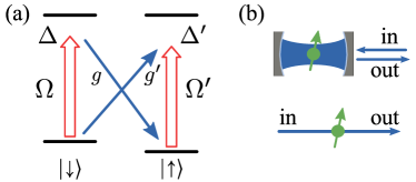
Figure 4: (Color online) (a) Level scheme of a TLS interacting with a quantum field (shown by thin blue lines) with the help of driving fields $\Omega$ and $\Omega^{\prime}$ (b) an adiabatic elimination of the intracavity field allows to consider the TLS directly interacting with the outside field.

We explain briefly how an interaction Hamiltonian $H_{\mathrm{int}}\propto\mathrm{i}[s\,a^{\dagger}(t)-s^{\dagger}a(t)]$ with $s_{1}=\sqrt{z(1+z)}\sigma_{1}^{+}+\sqrt{1-z}\sigma_{1}^{-}$ and $s_{2}=\sqrt{z(1+z)}\sigma_{2}^{+}-\sqrt{1-z}\sigma_{2}^{-}$ ($z\in[0,1]$), as required for continuous entanglement swapping, can be achieved. The same logic can be applied to other systems, such as a mechanical oscillator (see below). Consider an atom trapped in an optical cavity with stable ground states $|\!\downarrow\rangle$ and $|\!\uparrow\rangle$. The atom couples to the cavity through two transitions with single-photon Rabi frequencies $g$ and $g^{\prime}$, and is at the same time driven by two controllable laser fields at Rabi frequencies $\Omega$ and $\Omega^{\prime}$, as shown in Fig. 4(a). If the two-photon transitions are off-resonant with detunings $\Delta\gg g,\Omega$ and $\Delta^{\prime}\gg g^{\prime},\Omega^{\prime}$, one can eliminate the excited levels and engineer a tunable interaction of the ground states with the cavity field of the form

$$H_{\mathrm{eff}} =\mathrm{i}\left(\frac{\Omega g}{\Delta}\sigma^{+}c^{{\dagger}}+\frac{\Omega^{\prime}g^{\prime}}{\Delta^{\prime}}\sigma^{+}c-\mathrm{h.c.}\right)$$

$${=:}\,\mathrm{i}g_{\mathrm{eff}}\left(sc^{\dagger}-s^{\dagger}c\right).$$

Here $\sigma^{+}=|\!\!\uparrow\rangle\langle\downarrow\!\!|$ and $c$ is the cavity annihilation operator. By appropriate choice of the Rabi frequencies and detunings one can achieve any desired value of $z$ in the spin operator $s$, and at the same time set the effective coupling strength $g_{\mathrm{eff}}$. A tunable light–matter interaction based on two (effective) Raman transitions was recently demonstrated in Krauter et al. (2011). If the cavity decay (given by $\kappa$) is fast on the time scale of this effective coupling, the cavity field can be adiabatically eliminated. This gives rise to dynamics in which the spin effectively couples directly to the outside field, described by white noise operators $[a(t),a^{\dagger}(t^{\prime})]=\delta(t-t^{\prime})$ [Fig. 4(b)]. The Hamiltonian then is of the general form

$$H_{\mathrm{eff}}=\mathrm{i}\frac{g_{\mathrm{eff}}}{\sqrt{\kappa}}\left[sa^{\dagger}(t)-s^{\dagger}a(t)\right]$$

considered in the main article. The procedure of adiabatic elimination is discussed in some more detail for optomechanical systems in the following section.

Appendix E Continuous optomechanical teleportation

To derive Eq. (13) we start from the SME describing heterodyne detection of the optomechanical cavity’s output light. It can be obtained from equation (6) by replacing $s\rightarrow c_{\mathrm{c}}\,\mathrm{e}^{\mathrm{i}\Delta_{\mathrm{lo}}t}$, where $\Delta_{\mathrm{lo}}$ is the local oscillator detuning, and adding decoherence terms for the mechanical subsystem, which are due to its coupling to a thermal bath. After going into an interaction picture with $H_{0}=\omega_{\mathrm{m}}c_{\mathrm{m}}^{\dagger}c_{\mathrm{m}}+\Delta_{\mathrm{c}}c_{\mathrm{c}}^{\dagger}c_{\mathrm{c}}$ we can adiabatically eliminate the cavity mode, by expanding the equations in the small parameter $g/\kappa$ up to first order Doherty and Jacobs (1999); Wilson-Rae et al. (2008). Under this approximation and after setting $\Delta_{\mathrm{lo}}=\omega_{\mathrm{m}}$ the SME takes the form

$$\mathrm{d}\rho_{\mathrm{c}}=\mathcal{L}_{\mathrm{c}}\rho\mathrm{d}t-g^{2}\left[c_{\mathrm{m}}+c_{\mathrm{m}}^{\dagger},y\rho_{\mathrm{c}}-\rho_{\mathrm{c}}y^{\dagger}\right]\mathrm{d}t+\\ \sqrt{g^{2}\kappa/2}\left\{\mathcal{H}[-\mathrm{i}\mu\mathrm{e}^{\mathrm{i}\omega_{\mathrm{m}}t}y]\rho_{\mathrm{c}}\,\mathrm{d}W_{+}+\mathcal{H}[\nu\mathrm{e}^{\mathrm{i}\omega_{\mathrm{m}}t}y]\rho_{\mathrm{c}}\,\mathrm{d}W_{-}\right\}$$

where $\mathcal{L}_{\mathrm{m}}\rho=-\mathrm{i}[\omega_{\mathrm{m}}c_{\mathrm{m}}^{\dagger}c_{\mathrm{m}},\rho]+\gamma(\bar{n}+1)\mathcal{D}[c_{\mathrm{m}}]\rho+\gamma\bar{n}\mathcal{D}[c_{\mathrm{m}}^{\dagger}]\rho$, and $y=\eta_{-}c_{\mathrm{m}}+\eta_{+}c_{\mathrm{m}}^{\dagger}$. The steady-state mean amplitude of the intracavity field is $\langle c_{\mathrm{c}}\rangle=-\mathrm{i}g\langle y\rangle$. The heterodyne photocurrents can thus be obtained from (4) by the replacement $\langle s\rangle\rightarrow-\mathrm{i}g\langle y\rangle\mathrm{e}^{\mathrm{i}\omega_{\mathrm{m}}t}$, thus

$$I_{+} =-\mathrm{i}\sqrt{g^{2}\kappa/2}\langle y\,\mathrm{e}^{\mathrm{i}\omega_{\mathrm{m}}t}-\mathrm{h.c.}\rangle(t)+\xi_{+}(t)$$

$$I_{-} =\sqrt{g^{2}\kappa/2}\langle y\,\mathrm{e}^{\mathrm{i}\omega_{\mathrm{m}}t}+\mathrm{h.c.}\rangle(t)+\xi_{-}(t)$$

To apply the rotating wave approximation we go to the rotating frame of the mechanical oscillator (in the following denoted by $\tilde{\rho}_{\mathrm{c}}$) and take a time average over an interval $\delta t$, which comprises many mechanical periods, but is short on the system timescales in the rotating frame, i. e., $1/g\gg\delta t\gg 1/\omega_{\mathrm{m}}$. Under this assumption we can pull $\tilde{\rho}_{\mathrm{c}}$ out from under the integral and drop terms rotating at a frequency $\omega_{\mathrm{m}}$. At the same time we treat $\delta t$ as infinitesimal on the system’s timescale and therefore replace $\delta t\rightarrow\mathrm{d}t$. This leaves us with the equation

$$\mathrm{d}\tilde{\rho}_{\mathrm{c}}=\gamma_{-}\mathcal{D}[c_{\mathrm{m}}]\tilde{\rho}_{\mathrm{c}}\mathrm{d}t+\gamma_{+}\mathcal{D}[c_{\mathrm{m}}^{\dagger}]\tilde{\rho}_{\mathrm{c}}\mathrm{d}t\\ +\sqrt{g^{2}\kappa/2}\left\{\mathcal{H}[-\mathrm{i}\mu\eta_{+}c_{\mathrm{m}}^{\dagger}]\tilde{\rho}_{\mathrm{c}}\mathrm{d}W_{0+}+\mathcal{H}[\nu\eta_{+}c_{\mathrm{m}}^{\dagger}]\tilde{\rho}_{\mathrm{c}}\mathrm{d}W_{0-}\right\}.$$

We also introduced the time-averaged Wiener increments $\mathrm{d}W_{0\pm}=\int\mathrm{d}W_{\pm}$, which approximately fulfill (5), as far as $\tilde{\rho}_{\mathrm{c}}$ is concerned. In principle this equation contains additional measurement terms corresponding to sideband modes at frequencies $\pm 2\omega_{\mathrm{m}}$, which in a RWA are not correlated to the DC modes $\mathrm{d}W_{0\pm}$ and were therefore neglected. By renaming $\mathrm{d}W_{0\pm}\rightarrow\mathrm{d}W_{\pm}$ we arrive at (13). Note that by applying the RWA to the decoherence and the measurement terms consistently we assure that the resulting equation is a valid Belavkin equation Belavkin (1992).

To do feedback we do the same coarse-graining procedure for the photocurrents $I_{0\pm}=\int I_{\pm}\mathrm{d}t$, and find

$$I_{0+} =-\mathrm{i}\sqrt{g^{2}\kappa/2}\langle\eta_{+}c_{\mathrm{m}}^{\dagger}-\mathrm{h.c.}\rangle(t)+\xi_{+}(t),$$

$$I_{0-} =\sqrt{g^{2}\kappa/2}\langle\eta_{+}c_{\mathrm{m}}^{\dagger}+\mathrm{h.c.}\rangle(t)+\xi_{-}(t).$$

Within these approximations the system is equivalent to the generic case in the main text. Applying the same feedback procedure we obtain

$$\dot{\tilde{\rho}}_{\mathrm{m}}=\left\{\gamma(\bar{n}+1)\mathcal{D}[c_{\mathrm{m}}]+\gamma\bar{n}\mathcal{D}[c_{\mathrm{m}}^{\dagger}]\right\}\tilde{\rho}_{\mathrm{m}}\\ +(4g^{2}/\kappa)\left\{(1+\epsilon)\mathcal{D}[c_{\mathrm{m}}]+w_{3}\mathcal{D}[x_{\mathrm{m}}+p_{\mathrm{m}}]\right.\\ +\left.(w_{1}-w_{3}-1)\mathcal{D}[p_{\mathrm{m}}]+(w_{2}-w_{3}-1)\mathcal{D}[x_{\mathrm{m}}]\right\}\tilde{\rho}_{\mathrm{m}},$$

In view of the previous section we can diagonalize this equation to obtain

$$\dot{\tilde{\rho}}=\left\{\gamma(\bar{n}+1)\mathcal{D}[c_{\mathrm{m}}]+\gamma\bar{n}\mathcal{D}[c_{\mathrm{m}}^{\dagger}]\right\}\tilde{\rho}\\ +(4g^{2}/\kappa)\left\{\lambda_{1}(\epsilon)\mathcal{D}[J_{1}(\epsilon)]+\lambda_{2}(\epsilon)\mathcal{D}[J_{2}(\epsilon)]\right\}\tilde{\rho},$$ (1)

where $\lambda_{i}$ and $J_{i}$ are obtained from the eigenvalue decomposition of

$$\Lambda=\begin{pmatrix}w_{2}-\frac{1}{2}(1+\epsilon)&-w_{3}+\frac{\mathrm{i}}{2}(1+\epsilon)\\ -w_{3}-\frac{\mathrm{i}}{2}(1+\epsilon)&w_{1}-\frac{1}{2}(1+\epsilon)\end{pmatrix},$$

where $\epsilon=[1+(4\omega_{\mathrm{m}}/\kappa)^{2}]^{-1}$. In the limit $\epsilon\rightarrow 0$ Eq. (1) reduces to (8), apart from the decoherence terms of the mechanical subsystem, which counteract the squeezing of the mechanical mode by driving it towards a thermal state. Operating the protocol in a regime of strong cooperativity $g^{2}/\kappa\gg\gamma(\bar{n}+1)$ suppresses these perturbative effects.

References

- Bouwmeester et al. (1997) D. Bouwmeester, J.-W. Pan, K. Mattle, M. Eibl, H. Weinfurter, and A. Zeilinger, Nature 390, 575 (1997).
- Sherson et al. (2006) J. F. Sherson, H. Krauter, R. K. Olsson, B. Julsgaard, K. Hammerer, I. Cirac, and E. S. Polzik, Nature 443, 557 (2006).
- Riebe et al. (2004) M. Riebe, H. Häffner, C. F. Roos, W. Hänsel, J. Benhelm, G. P. T. Lancaster, T. W. Körber, C. Becher, F. Schmidt-Kaler, D. F. V. James, and R. Blatt, Nature 429, 734 (2004).
- Barrett et al. (2004) M. D. Barrett, J. Chiaverini, T. Schaetz, J. Britton, W. M. Itano, J. D. Jost, E. Knill, C. Langer, D. Leibfried, R. Ozeri, and D. J. Wineland, Nature 429, 737 (2004).
- Bushev et al. (2006) P. Bushev, D. Rotter, A. Wilson, F. Dubin, C. Becher, J. Eschner, R. Blatt, V. Steixner, P. Rabl, and P. Zoller, Physical Review Letters 96, 043003 (2006).
- Kubanek et al. (2009) A. Kubanek, M. Koch, C. Sames, A. Ourjoumtsev, P. W. H. Pinkse, K. Murr, and G. Rempe, Nature 462, 898 (2009).
- Koch et al. (2010) M. Koch, C. Sames, A. Kubanek, M. Apel, M. Balbach, A. Ourjoumtsev, P. W. H. Pinkse, and G. Rempe, Physical Review Letters 105, 173003 (2010).
- Sayrin et al. (2011) C. Sayrin, I. Dotsenko, X. Zhou, B. Peaudecerf, T. Rybarczyk, S. Gleyzes, P. Rouchon, M. Mirrahimi, H. Amini, M. Brune, J.-M. Raimond, and S. Haroche, Nature 477, 73 (2011).
- Haroche and Raimond (2006) S. Haroche and J.-M. Raimond, Exploring the Quantum: Atoms, Cavities, and Photons (OUP Oxford, 2006).
- Smith et al. (2006) G. A. Smith, A. Silberfarb, I. H. Deutsch, and P. S. Jessen, Physical Review Letters 97, 180403 (2006).
- Chaudhury et al. (2007) S. Chaudhury, S. Merkel, T. Herr, A. Silberfarb, I. H. Deutsch, and P. S. Jessen, Physical Review Letters 99, 163002 (2007).
- Krauter et al. (2011) H. Krauter, C. A. Muschik, K. Jensen, W. Wasilewski, J. M. Petersen, J. I. Cirac, and E. S. Polzik, Physical Review Letters 107, 080503 (2011).
- Vijay et al. (2012) R. Vijay, C. Macklin, D. H. Slichter, S. J. Weber, K. W. Murch, R. Naik, A. N. Korotkov, and I. Siddiqi, Nature 490, 77 (2012).
- Ristè et al. (2013) D. Ristè, M. Dukalski, C. A. Watson, G. de Lange, M. J. Tiggelman, Y. M. Blanter, K. W. Lehnert, R. N. Schouten, and L. DiCarlo, Deterministic entanglement of superconducting qubits by parity measurement and feedback, arXiv e-print 1306.4002 (2013).
- Arcizet et al. (2006) O. Arcizet, P.-F. Cohadon, T. Briant, M. Pinard, A. Heidmann, J.-M. Mackowski, C. Michel, L. Pinard, O. Français, and L. Rousseau, Physical Review Letters 97, 133601 (2006).
- Corbitt et al. (2007) T. Corbitt, C. Wipf, T. Bodiya, D. Ottaway, D. Sigg, N. Smith, S. Whitcomb, and N. Mavalvala, Physical Review Letters 99, 160801 (2007).
- Mow-Lowry et al. (2008) C. M. Mow-Lowry, A. J. Mullavey, S. Goßler, M. B. Gray, and D. E. McClelland, Physical Review Letters 100, 010801 (2008).
- Abbott et al. (2009) B. Abbott, R. Abbott, R. Adhikari, P. Ajith, B. Allen, G. Allen, R. Amin, S. B. Anderson, W. G. Anderson, and M. A. Arain, New Journal of Physics 11, 073032 (2009).
- Belavkin (1980) V. Belavkin, Radio Eng Electron Physics 25, 1445–1453 (1980).
- Hudson and Parthasarathy (1984) R. L. Hudson and K. R. Parthasarathy, Communications in Mathematical Physics 93, 301 (1984).
- Gardiner and Collett (1985) C. W. Gardiner and M. J. Collett, Physical Review A 31, 3761 (1985).
- Gardiner et al. (1992) C. W. Gardiner, A. S. Parkins, and P. Zoller, Physical Review A 46, 4363 (1992).
- Wiseman and Milburn (1993a) H. M. Wiseman and G. J. Milburn, Physical Review A 47, 642 (1993a).
- Wiseman (1994) H. M. Wiseman, Physical Review A 49, 2133 (1994).
- Doherty et al. (2000) A. C. Doherty, S. Habib, K. Jacobs, H. Mabuchi, and S. M. Tan, Physical Review A 62, 012105 (2000).
- Hopkins et al. (2003) A. Hopkins, K. Jacobs, S. Habib, and K. Schwab, Physical Review B 68, 235328 (2003).
- Jacobs and Steck (2006) K. Jacobs and D. A. Steck, Contemporary Physics 47, 279 (2006).
- Bouten et al. (2007) L. Bouten, R. Van Handel, and M. R. James, SIAM Journal on Control and Optimization 46, 2199 (2007).
- Parthasarathy (1992) K. R. Parthasarathy, An Introduction to Quantum Stochastic Calculus (Springer, 1992).
- Carmichael (1993) H. Carmichael, An open systems approach to quantum optics (Springer-Verlag, 1993).
- Gardiner and Zoller (2004) C. W. Gardiner and P. Zoller, Quantum noise, 3rd ed. (Springer, 2004).
- Wiseman and Milburn (2009) H. M. Wiseman and G. J. Milburn, Quantum Measurement and Control (Cambridge University Press, 2009).
- Barchielli and Gregoratti (2009) A. Barchielli and M. Gregoratti, Quantum Trajectories and Measurements in Continuous Time: The Diffusive Case (Springer, 2009).
- Note (1) We here use the term ‘Bell measurement’ in the context of continuous variables, where it describes the measurement projecting onto the maximally entangled EPR states.
- Vollbrecht et al. (2011) K. G. H. Vollbrecht, C. A. Muschik, and J. I. Cirac, Physical Review Letters 107, 120502 (2011).
- Chen (2013) Y. Chen, Journal of Physics B: Atomic, Molecular and Optical Physics 46, 104001 (2013).
- Aspelmeyer et al. (2013) M. Aspelmeyer, T. J. Kippenberg, and F. Marquardt, arXiv:1303.0733 (2013).
- Murch et al. (2008) K. W. Murch, K. L. Moore, S. Gupta, and D. M. Stamper-Kurn, Nature Physics 4, 561 (2008).
- Teufel et al. (2011) J. D. Teufel, T. Donner, D. Li, J. W. Harlow, M. S. Allman, K. Cicak, A. J. Sirois, J. D. Whittaker, K. W. Lehnert, and R. W. Simmonds, Nature 475, 359 (2011).
- Chan et al. (2011) J. Chan, T. P. M. Alegre, A. H. Safavi-Naeini, J. T. Hill, A. Krause, S. Groblacher, M. Aspelmeyer, and O. Painter, Nature 478, 89 (2011).
- Brooks et al. (2012) D. W. C. Brooks, T. Botter, S. Schreppler, T. P. Purdy, N. Brahms, and D. M. Stamper-Kurn, Nature 488, 476 (2012).
- Purdy et al. (2013) T. P. Purdy, R. W. Peterson, and C. A. Regal, Science 339, 801 (2013).
- Safavi-Naeini et al. (2013) A. H. Safavi-Naeini, S. Gröblacher, J. T. Hill, J. Chan, M. Aspelmeyer, and O. Painter, Nature 500, 185 (2013).
- Goetsch and Graham (1994) P. Goetsch and R. Graham, Physical Review A 50, 5242 (1994).
- Wiseman and Milburn (1993b) H. M. Wiseman and G. J. Milburn, Physical Review Letters 70, 548 (1993b).
- Vidal and Werner (2002) G. Vidal and R. F. Werner, Physical Review A 65, 032314 (2002).
- Müller-Ebhardt et al. (2008) H. Müller-Ebhardt, H. Rehbein, R. Schnabel, K. Danzmann, and Y. Chen, Physical Review Letters 100, 013601 (2008).
- Kraus et al. (2008) B. Kraus, H. P. Büchler, S. Diehl, A. Kantian, A. Micheli, and P. Zoller, Physical Review A 78, 042307 (2008).
- Bose et al. (1999) S. Bose, P. L. Knight, M. B. Plenio, and V. Vedral, Physical Review Letters 83, 5158 (1999).
- Duan and Kimble (2003) L.-M. Duan and H. J. Kimble, Physical Review Letters 90, 253601 (2003).
- Simon and Irvine (2003) C. Simon and W. T. M. Irvine, Physical Review Letters 91, 110405 (2003).
- Browne et al. (2003) D. E. Browne, M. B. Plenio, and S. F. Huelga, Physical Review Letters 91, 067901 (2003).
- Campbell and Benjamin (2008) E. T. Campbell and S. C. Benjamin, Physical Review Letters 101, 130502 (2008).
- Vollbrecht and Cirac (2009) K. G. H. Vollbrecht and J. I. Cirac, Physical Review A 79, 042305 (2009).
- Santos et al. (2012) M. F. Santos, M. Terra Cunha, R. Chaves, and A. R. R. Carvalho, Physical Review Letters 108, 170501 (2012).
- Cirac et al. (1997) J. I. Cirac, P. Zoller, H. J. Kimble, and H. Mabuchi, Physical Review Letters 78, 3221 (1997).
- Pellizzari (1997) T. Pellizzari, Physical Review Letters 79, 5242 (1997).
- van Enk et al. (1997) S. J. van Enk, J. I. Cirac, and P. Zoller, Physical Review Letters 78, 4293 (1997).
- Parkins and Kimble (2000) A. S. Parkins and H. J. Kimble, Physical Review A 61, 052104 (2000).
- Mancini and Bose (2001) S. Mancini and S. Bose, Physical Review A 64, 032308 (2001).
- Clark et al. (2003) S. Clark, A. Peng, M. Gu, and S. Parkins, Physical Review Letters 91, 177901 (2003).
- Kraus and Cirac (2004) B. Kraus and J. I. Cirac, Physical Review Letters 92, 013602 (2004).
- Mancini and Bose (2004) S. Mancini and S. Bose, Physical Review A 70, 022307 (2004).
- Raimond et al. (2001) J. M. Raimond, M. Brune, and S. Haroche, Reviews of Modern Physics 73, 565 (2001).
- Miller et al. (2005) R. Miller, T. E. Northup, K. M. Birnbaum, A. Boca, A. D. Boozer, and H. J. Kimble, Journal of Physics B: Atomic, Molecular and Optical Physics 38, S551 (2005).
- Walther et al. (2006) H. Walther, B. T. H. Varcoe, B.-G. Englert, and T. Becker, Reports on Progress in Physics 69, 1325 (2006).
- Girvin et al. (2009) S. M. Girvin, M. H. Devoret, and R. J. Schoelkopf, Physica Scripta T137, 014012 (2009).
- Vetsch et al. (2010) E. Vetsch, D. Reitz, G. Sagué, R. Schmidt, S. T. Dawkins, and A. Rauschenbeutel, Physical Review Letters 104, 203603 (2010).
- Goban et al. (2012) A. Goban, K. S. Choi, D. J. Alton, D. Ding, C. Lacroûte, M. Pototschnig, T. Thiele, N. P. Stern, and H. J. Kimble, Physical Review Letters 109, 033603 (2012).
- Hammerer et al. (2010) K. Hammerer, A. S. Sørensen, and E. S. Polzik, Reviews of Modern Physics 82, 1041 (2010).
- Saffman et al. (2010) M. Saffman, T. G. Walker, and K. Mølmer, Reviews of Modern Physics 82, 2313 (2010).
- Note (2) With appropriate feedback a Bell state is also achieved in the limit .
- Wolf et al. (2007) M. M. Wolf, D. Pérez-García, and G. Giedke, Physical Review Letters 98, 130501 (2007).
- Doherty and Jacobs (1999) A. C. Doherty and K. Jacobs, Physical Review A 60, 2700 (1999).
- Wilson-Rae et al. (2007) I. Wilson-Rae, N. Nooshi, W. Zwerger, and T. J. Kippenberg, Physical Review Letters 99, 093901 (2007).
- Marquardt et al. (2007) F. Marquardt, J. P. Chen, A. A. Clerk, and S. M. Girvin, Physical Review Letters 99, 093902 (2007).
- Belavkin (1999) V. Belavkin, Reports on Mathematical Physics 43, A405 (1999).
- Demchenko and Vyatchanin (2013) A. A. Demchenko and S. P. Vyatchanin, arXiv:1303.4188 (2013).
- Mancini et al. (2003) S. Mancini, D. Vitali, and P. Tombesi, Physical Review Letters 90, 137901 (2003).
- Zhang et al. (2003) J. Zhang, K. Peng, and S. L. Braunstein, Physical Review A 68, 013808 (2003).
- Romero-Isart et al. (2011) O. Romero-Isart, A. C. Pflanzer, M. L. Juan, R. Quidant, N. Kiesel, M. Aspelmeyer, and J. I. Cirac, Physical Review A 83, 013803 (2011).
- Hofer et al. (2011) S. G. Hofer, W. Wieczorek, M. Aspelmeyer, and K. Hammerer, Physical Review A 84, 052327 (2011).
- Wilson-Rae et al. (2008) I. Wilson-Rae, N. Nooshi, J. Dobrindt, T. J. Kippenberg, and W. Zwerger, New Journal of Physics 10, 095007 (2008).
- Note (3) Note that the mechanical resonance frequency shifts due to the optical spring effect. The rotating frame will therefore rotate at a frequency .
- Belavkin (1992) V. P. Belavkin, Journal of Multivariate Analysis 42, 171 (1992).