Amendable Gaussian channels: restoring entanglement via a unitary filter

Abstract

We show that there exist Gaussian channels which are amendable. A channel is amendable if when applied twice is entanglement breaking while there exists a unitary filter such that, when interposed between the first and second action of the map, prevents the global transformation from being entanglement breaking [Phys. Rev. A 86, 052302 (2012)]. We find that, depending on the structure of the channel, the unitary filter can be a squeezing transformation or a phase shift operation. We also propose two realistic quantum optics experiments where the amendability of Gaussian channels can be verified by exploiting the fact that it is sufficient to test the entanglement breaking properties of two mode Gaussian channels on input states with finite energy (which are not maximally entangled).

Introduction

Quantum states formally represent the addressable information content about the system they describe. During their evolution quantum systems may suffer the presence of noise, for instance due to the interaction with another system, generally referred as an external environment. This may cause a loss of information on the system, and leads to a modification from its initial to its final state. In quantum communication theory, stochastic channels, that is Completely Positive Trace Preserving (CPT) mappings, provide a formal description of the noise affecting the system during its evolution. The most detrimental form of noise from the point of view of quantum information, is described by the so-called Entanglement Breaking (EB) maps EBT . These maps when acting on a given system destroy any entanglement that was initially present between the system itself and an arbitrary external ancilla. Accordingly they can be simulated as a two–stage process where a first party makes a measurement on the input state and sends the outcome, via a classical channel, to a second party who then re-prepares the system of interest in a previously agreed state holevoEBT .

For continuous variable quantum systems cv , like optical or mechanical modes, there is a particular class of CPT maps which is extremely important: the class of Gaussian channels gaussian ; review . Almost every realistic transmission line (e.g. optical fibers, free space communication, etc.) can be described as a Gaussian channel. In this context the notion of EB channels has been introduced and characterized in Ref. HOLEVOEBG . Gaussian channels, even if they are not entanglement breaking, usually degrade quantum coherence and tend to decrease the initial entanglement of the state buono . One may try to apply error correction procedures based on Gaussian encoding and decoding operations acting respectively on the input and output states of the map plus possibly some ancillary systems. This however has been shown to be useless nogo , in the sense that Gaussian procedures cannot augment the entanglement transmitted through the channel (no-go theorem for Gaussian Quantum Error Correction). Here we point out that such lack of effectiveness doesn’t apply when we allow Gaussian recovering operations to act between two successive applications of the same map on the system. Specifically our approach is based on the notion of amendable channels introduced in mucritico , whose definition derives from the generalization of the class of EB maps (Gaussian and not) to the class of EB channels of order $n$. The latter are maps $\Phi$ which, even if not necessarily EB, become EB after $n$ iterative applications on the system (in other words, indicating with “$\circ$” the composition of super-operator, $\Phi$ is said to be EB of order $n$ if $\Phi^{n}:=\Phi\circ\Phi\circ\cdots\circ\Phi$ is EB while $\Phi^{n-1}$ is not). We therefore say that a map is amendable if it is EB of order 2, and there exists a second channel (called filtering map) such that when interposed between the two actions of the initial map, prevents the global one to be EB. In this context we show that there exist Gaussian EB channels of order $2$ which are amendable through the action of a proper Gaussian unitary filter (i.e. whose detrimental action can be stopped by performing an intermediate, recovering Gaussian transformation).

The paper is structured as follows. In Section I we focus on the formalism of Gaussian channels, the characterization of EB Gaussian channels and their main properties. In Section II we explicitly define two types of channels which are amendable via a squeezing operation and a phase shifter respectively. For each channel we also propose a simple experiment based on finite quantum resources and feasible within current technology.

I Entanglement breaking Gaussian channels

Let us briefly set some standard notation. A state $\rho$ of a bosonic system with $f$ degrees of freedom is Gaussian if its characteristic function $\phi_{\rho}(z)=\mathrm{Tr}[\rho W(z)]$ has a Gaussian form gaussian ,

$$\phi_{\rho}(\vec{z})=e^{i{\langle\vec{R}\rangle}_{\rho}^{\top}\vec{z}-\frac{1}{2}\vec{z}^{\top}{\ \mathbf{V}_{\rho}}\vec{z}}\,.$$ (1)

$W(\vec{z})$ is the unitary Weyl operator defined on the real vector space $\mathbb{R}^{2f}$, $W(\vec{z}):=\exp[i\vec{R}\cdot\Delta\vec{z}]$, where

$$\Delta=\bigoplus_{i=1}^{f}\left(\begin{array}[]{cc}0&1\\ -1&0\end{array}\right)$$ (2)

is the symplectic form, $\vec{R}=\{Q_{1},P_{1},\ldots,Q_{f},P_{f}\}$ and $Q_{i}$, $P_{i}$ are the canonical observables for the bosonic system. $\langle\vec{R}\rangle_{\rho}$ is vector of the expectation values of $\vec{R}$, and $\mathbf{V}_{\rho}$ is the covariance matrix

$$[\mathbf{V}_{\rho}]_{ij}=\frac{\langle R_{i}R_{j}+R_{j}R_{i}\rangle_{\rho}}{2}-\langle R_{i}\rangle_{\rho}\langle R_{j}\rangle_{\rho}\,.$$ (3)

A CPT map $\Phi$ is called Gaussian if it preserves the Gaussian character of the states, and can be conveniently described by the triplet $(K,l,\beta)$, $l\in\mathbb{R}^{2f}$ and $K$, $\beta$ being $2f\times 2f$ matrices, which fulfill the condition

$$\beta\geq\pm i[\Delta-K^{\top}\Delta K]/2,\quad$$ (4)

and act on ${\langle\vec{R}\rangle}_{\rho}$ and $\mathbf{V}_{\rho}$ as

$$\mathbf{V}_{\rho} \to {\mathbf{V}_{\Phi[\rho]}}=K^{\top}\mathbf{V}_{\rho}K+\beta\,$$ (5)

$${\langle\vec{R}\rangle}_{\rho} \to {\langle\vec{R}\rangle}_{\Phi[\rho]}=K^{\top}{\langle\vec{R}\rangle}_{\rho}+l.$$ (6)

A special subset of Gaussian channels is constituted by the unitary Gaussian transformations, characterized by having $\beta=0$: they include multi-mode squeezing, phase shifts, displacement transformations and products among them.

The composition of two Gaussian maps, $\Phi=\Phi_{2}\circ\Phi_{1}$, described by $(K_{1},l_{1},\beta_{1})$ and $(K_{2},l_{2},\beta_{2})$ respectively, is still a Gaussian map whose parameters are given by

$$\Phi_{2}\circ\Phi_{1}\longrightarrow\left\{\begin{array}[]{l}K=K_{1}K_{2}\\ l=K_{2}^{\top}l_{1}+l_{2}\\ \beta=K_{2}^{\top}\beta_{1}K_{2}+\beta_{2}.\end{array}\right.$$ (10)

Finally, a Gaussian map $\Phi$ is entanglement-breaking HOLEVOEBG if and only if its matrix $\beta$ can be expressed as

$$\beta=\alpha+\nu,$$ (11)

with

$$\alpha\geq\frac{i}{2}\Delta,\quad\mbox{and}\quad\nu\geq\frac{i}{2}K^{\top}\Delta K.$$ (12)

I.1 One-mode attenuation channels

One-mode attenuation channels $\Phi_{\mathrm{At}}(N_{0},\eta)$ are special examples of Gaussian mappings such that:

$$K_{\mathrm{At}} = \sqrt{\eta}\;\openone$$ (13)

$$l_{\mathrm{At}} = 0$$ (14)

$$\beta_{\mathrm{At}} = \left(N_{0}+\frac{1-\eta}{2}\right)\openone$$ (15)

where $\openone=\left(\begin{array}[]{cc}1&0\\ 0&1\end{array}\right)$, $0\leq\eta\leq 1$ and $N_{0}\geq 0$. This transformation can be described in terms of a coupling between the system and a thermal Bosonic bath with mean photon number $N=N_{0}/(1-\eta)$, mediated by a beam splitter of transmissivity $\eta$. In Ref. mucritico the EB properties of the maps $\Phi_{\mathrm{At}}(N_{0},\eta)$ under channel iteration were studied as a function of the parameters $\eta^{2}$ and $N_{0}$. For completeness we report these findings in Fig. 1. In the plot the solid lines represent the lower boundaries between the regions which identify the set of transformations $\Phi_{\mathrm{At}}(N_{0},\eta)$ which are EB of order $n$. They are analytically identified by the inequalities

$$N_{0}\geq\frac{\eta^{n}}{\sum_{j=0}^{n-1}\eta^{j}}\,,$$ (16)

or, in terms of the parameter $N$ which gauges the bath average photon number, by

$$N\geq(1-\eta)\frac{\eta^{n}}{\sum_{j=0}^{n-1}\eta^{j}}\,.$$ (17)

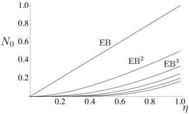
Figure 1: Lower boundary of the regions such that $\Phi_{{\mathrm{At}}}\in\mathrm{EB}^{n}$, in the parameter space $\{\eta,N_{0}\}$.

Notice that for $N=0$, $\Phi_{{\mathrm{At}}}^{n}\notin{\mathrm{EB}}$ for all finite $n$, that is if the system is coupled with the vacuum (zero photons) the reiterative application of the map, represented by the action of a beam-splitter on the input signal, does not destroy the entanglement between the system and any other ancilla with which it is maximally entangled before the action of the map.

I.2 Certifying that a channel is entanglement breaking with non ideal resources.

It is a well known fact that a map $\Phi$ is EB if and only if when applied to one side of a maximally entangled state it produces a separable state EBT . This fact gives an operationally well defined experimental procedure for characterizing the EB property of a channel $\Phi$ based on the ability of preparing a maximally entangled state to be used as probing state for the map. Unfortunately however, while feasible for finite dimensional systems, in a continuous variable setting this approach is clearly problematic due to the physical impossibility of preparing such an ideal probe state since it would require an infinite amount of energy. Quite surprisingly, the following property will avoid this experimental issue.

Property (equivalent test states). Given $\{|i\rangle;i=1,\cdots,d\}$ an orthonormal set, let $\omega=\sum_{i,i^{\prime}=1}^{d}|i\,i\rangle\langle i^{\prime}\,i^{\prime}|$ be an un-normalized maximally entangled state and $\sigma$ a full-rank $d\times d$ density matrix. Then the (normalized) state

$$\tilde{\omega}=(\sigma^{1/2}\otimes\openone)\omega(\sigma^{1/2}\otimes\openone)$$ (18)

is a valid resource equivalent to $\omega$ in the sense that a channel $\Phi$ is EB if and only if $(\openone\otimes\Phi)(\tilde{\omega})$ is separable.

Proof. We already know that $\Phi$ is EB if and only if $f=(\openone\otimes\Phi)(\omega)$ is separable EBT . We need to show that $f$ is separable if and only if $\tilde{f}=(\openone\otimes\Phi)(\tilde{\omega})$ is separable. This must be true because the two states differ only by a local CP map which cannot produce entanglement namely: $\tilde{f}=(\sigma^{1/2}\otimes\openone)f(\sigma^{1/2}\otimes\openone)$ and $f=(\sigma^{-1/2}\otimes\openone)\tilde{f}(\sigma^{-1/2}\otimes\openone)$.

The same property can be extended to continuous variable systems where $\omega$ is not normalizable but it can still be consistently interpreted as a distribution holevochoi . Now, let us consider a two-mode squeezed vacuum (TMSV) state with finite squeezing parameter $r^{\prime}$, i.e.

$$\tilde{\omega}=\frac{1}{(\cosh r^{\prime})^{2}}\sum_{i,i^{\prime}=0}^{\infty}(\tanh r^{\prime})^{i+i^{\prime}}|i\rangle_{1}\langle i^{\prime}|\otimes|i\rangle_{2}\langle i^{\prime}|,$$ (19)

where $\{|i\rangle;i=1,2,\cdots\}$ is now the Fock basis. It can be expressed in the form of Eq. (18) by choosing

$$\sigma=\text{tr}_{2}\{\tilde{\omega}\}=\frac{1}{(\cosh r^{\prime})^{2}}\sum_{i=0}^{\infty}(\tanh r^{\prime})^{2i}|i\rangle_{1}\langle i|$$ (20)

and therefore the state $\tilde{\omega}$ is a valid resource for the EB test. The previous property implies that it is sufficient to test the action of a channel on a two-mode squeezed state with arbitrary finite entanglement in order to verify if the channel is EB or not. Surprisingly, even a tiny amount of entanglement is in principle enough for the test. However, because of experimental detection noise and imperfections, a larger value of $r^{\prime}$ may be preferable as it allows for a clean-cut discrimination.

The previous results are obviously extremely important from an experimental point of view since, for single mode Gaussian channels, one can apply the following operational procedure:

• Prepare a realistic two-mode squeezed vacuum state $\tilde{\omega}$ with a finite value of $r^{\prime}$,

• Apply the channel $\Phi$ to one mode of the entangled state resulting in $\tilde{f}=(\openone\otimes\Phi)(\tilde{\omega})$,

• Check if the state $\tilde{f}$ is entangled or not.

Probably the experimentally most direct way of witnessing the entanglement of $\tilde{f}$ is to apply the so-called product criterion prodcrit . In this case, entanglement is detected whenever

$$\mathcal{W}=\left\langle Q^{2}\right\rangle\left\langle P^{2}\right\rangle<\frac{1}{4}$$ (21)

with

$$Q=\frac{Q_{1}+Q_{2}}{\sqrt{2}},\qquad P=\frac{P_{1}-P_{2}}{\sqrt{2}}\,.$$ (22)

We indicate with $Q_{i}$ and $P_{i}$, $i=1,2$, the position and momentum quadratures associated to each mode of the twin beam. If inequality (21) is satisfied, $\tilde{f}$ is entangled and so $\Phi$ is not EB. This test, is a witness but it does not provide a conclusive separability proof. For this reason it is useful to compare it with a necessary and sufficient criterion. We will use the logarithmic negativity $E_{\mathcal{N}}$, which is an entanglement measure quantifying the violation of the $PPT$ separability criterion PPT . Let $\mathbf{V}_{\tilde{\omega}}$ be the covariance matrix of $\tilde{\omega}$ written in the block form

$$\mathbf{V}_{\rho}=\begin{pmatrix}\mathbf{A}&\mathbf{C}\\ \mathbf{C^{\top}}&\mathbf{B}\end{pmatrix}\,.$$ (23)

The entanglement negativity $E_{\mathcal{N}}$ is a function of the four invariants under local symplectic transformations $\det[\mathbf{A}],\det[\mathbf{B}],\det[\mathbf{C}],\det[\mathbf{V}_{\rho}]$ and can be analytically computed gaussian :

$$E_{\mathcal{N}} = \max\{-\ln(2\nu),0\}$$ (24)

$$\nu = \sqrt{\frac{\Sigma-\sqrt{\Sigma^{2}-4\det[\mathbf{V}_{\rho}]}}{2}}$$ (25)

where $\Sigma=\det[\mathbf{A}]+\det[\mathbf{B}]-2\det[\mathbf{C}]$. Notice that $\nu$ is the minimum symplectic eigenvalue of the partially transposed state and can be interpreted as an optimal product creterion since we have that $\tilde{f}$ is entangled if and only if

$$\nu^{2}<\frac{1}{4}\,,$$ (26)

while Eq. (21) is only a sufficient condition.

Both tests Eq. (21) and (26) will be used for assessing, in the next section, the entanglement breaking property of two possible realization of amendable Gaussian channels. We note that, direct simultaneous measurements, in a dual-homodyne set-up, on the entangled sub-systems allow a direct evaluation of the product criterion dualhomo . While, the experimental evaluation of $E_{\mathcal{N}}$ requires the reconstruction of the bipartite system covariance matrix that in many cases can be gained by a single homodyne singlehomo .

II Amendable gaussian maps

In this section we aim to prove the existence of amendable Gaussian maps constructing explicit examples and propose experimental setups that would allow one to implement and test them. To do so we will look for Gaussian single mode maps $\mathcal{U}$ and $\Phi$, where $\mathcal{U}$ is unitary, such that

$$\Phi\circ\mathcal{U}\circ\Phi \in {\mathrm{EB}}\;,$$ (27)

$$\Phi^{2} \notin {\mathrm{EB}}\;,$$ (28)

(notice that the second condition requires that $\Phi$ cannot be EB). Under these assumptions, it follows that the channel $\Phi^{\mathcal{U}}=\mathcal{U}\circ\Phi$ is an EB map of order 2 which can be amended by the unitary filter $\mathcal{U}^{\dagger}$. Indeed exploiting the fact that local unitary transformation cannot alter the entanglement, the above expressions imply:

$$\Phi^{\mathcal{U}}\circ\Phi^{\mathcal{U}}=\mathcal{U}\circ\Phi\circ\mathcal{U}\circ\Phi \in {\mathrm{EB}}\;,$$ (29)

$$\Phi^{\mathcal{U}}\circ\mathcal{U}^{\dagger}\circ\Phi^{\mathcal{U}}=\mathcal{U}\circ\Phi^{2} \notin {\mathrm{EB}}\;.$$ (30)

Even though (27), (28) and (29), (30) are formally equivalent it turns out that the former relations are easier to be implemented experimentally. For this reason in the following we will focus on such scenario.

II.1 Example 1: Beam splitter-squeezing-beam splitter

Here we provide our first example of a channel $\Phi$ and of a unitary transformation $\mathcal{U}$ fulfilling Eqs. (27) and (28). We will consider two mode Gaussian maps. By exploiting the property explained in Sec. I.2 regarding the equivalence of test states, without loss of generality we will apply our channels to twin-beam states with finite squeezing parameter, that is with finite energy, rather then to maximally entangled states which would require an infinite amount of energy to be realized. Eqs. (27) and (28) will be implemented by the two setups of Fig. 2:

• The first one (setup $1$) is used to realize the transformation $\Phi\circ\mathcal{U}\circ\Phi$. It consists in an optical squeezer, implementing the unitary $\mathcal{U}$, coupled on both sides with a beam-splitter (one for each side) of transmissivity $\eta$.

• The second setup (setup $2$ of Fig. 2) instead is used to realize the transformation $\Phi\circ\Phi$: it is obtained from the first by removing the squeezer between the beam splitters.

As anticipated we will use $|TMSV\rangle$ states as entangled probes. The aim of the section is to show that by properly choosing the system parameters, the squeezing and the beam-splitter transmissivities, it is possible to realize an amendable Gausssian channel.

The transformation induced by the beam splitter can be described by an attenuation map with $N_{0}=0$, $\Phi_{\mathrm{BS}_{1}}(\eta):=\Phi_{\mathrm{At}}(0,\eta)$. On the other hand, we indicate as $\mathcal{S}_{1}(r)$ the unitary map depending on the real parameter $r$, referring to the action of an optical squeezer

$$K_{\mathcal{S}_{1}}(r) = \begin{pmatrix}e^{r}&0\\ 0&e^{-r}\end{pmatrix}$$ (31)

$$l_{\mathcal{S}_{1}} = 0$$ (32)

$$\beta_{\mathcal{S}_{1}} = 0\,.$$ (33)

We set the initial state of the two modes to be a twin-beam $\rho_{0}(r^{\prime})=|TMSV\,(r^{\prime})\,\rangle\langle TMSV\,(r^{\prime})\,|$, with covariance matrix given by

$$\mathbf{V}_{2s}(r^{\prime})=\frac{1}{2}\begin{pmatrix}\cosh{r^{\prime}}\openone&\sinh r^{\prime}\sigma_{z}\\ \sinh r^{\prime}\sigma_{z}&\cosh r^{\prime}\openone\end{pmatrix}\,.$$ (34)

The states at the output of our two setups are described by the following 2-mode density matrices, $\rho_{\Phi_{1}}:=(\Phi_{1}\otimes I)[\rho_{0}]$ and $\rho_{\Phi_{2}}:=(\Phi_{2}\otimes I)[\rho_{0}]$ with

$$\Phi_{1}:=\Phi_{1}(\eta,r)=\Phi_{\mathrm{At}}(\eta)\circ\mathcal{S}_{1}(r)\circ\Phi_{\mathrm{At}}(\eta)\;,$$ (35)

$$\Phi_{2}:=\Phi_{2}(\eta)=\Phi_{\mathrm{At}}(\eta)\circ\Phi_{\mathrm{At}}(\eta)\;.$$ (36)

We stress that $\Phi_{1}$ and $\Phi_{2}$ act only on one of the two modes of the incoming twin-beam.

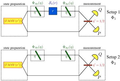
Figure 2: (Color online) Schematic of the experimental proposal discussed in Sec. II.1. Both setups are divided in three stages: a $|TMSV\rangle$ state is prepared, the desired sequence of channels is applied to one mode of the entangled probe, and finally the output state is measured. The beam-splitters implement the attenuation channels $\Phi_{At}(\eta)$ of Eqs. (35), (36) which represent the transformations $\Phi$ of Eqs. (27), (28), while the squeezing transformation $\mathcal{S}_{1}(r)$ implements the unitary $\mathcal{U}$.

The entanglement properties of the two setups can be established by applying the criterion (11)-(12) to $\Phi_{1,2}$. As already recalled, in mucritico it was shown that $\Phi_{2}=\Phi_{\mathrm{At}}^{2}(\eta)$ never becomes ${\mathrm{EB}}$ for any value of the transmissivity $\eta$. On the contrary, it can be shown that $\Phi_{1}$, given by

$$K_{1} = \eta K_{\mathcal{S}_{1}}(r)$$ (37)

$$l_{1} = 0$$ (38)

$$\beta_{1} = \left(\frac{1-\eta}{2}\right)(\eta K_{\mathcal{S}_{1}}(r)^{2}+\openone)\,,$$ (39)

is EB if and only if

$$\eta\leq\tilde{\eta}(r)=\frac{1}{2}\left(\cosh(2r)-\sqrt{2\cosh(2r)-1}\right)\text{csch}^{2}(r)$$ (40)

or equivalently

$$r\geq\tilde{r}(\eta)=\frac{1}{2}\cosh^{-1}\left(\frac{\eta^{2}+1}{(\eta-1)^{2}}\right)\,.$$ (41)

In Fig. 3 we report plots of $\tilde{\eta}$ vs. $r$ and $\tilde{r}$ vs. $\eta$ to better visualize the EB regions for the two parameters.

Figure 3: Lower (a) /Upper (b) bound of the ${\mathrm{EB}}$ region for $\Phi_{1}$. Notice that in (a) $r$ diverges in the limit of transmissivity $1$ for the beam splitter, and in the complementary plot (b) the transmissivity reaches $1$ asymptotically for $r\to\infty$.

It follows then, that for all values of $\eta$ and $r$ fulfilling the condition (40) [or its equivalent version (41)] the channel concatenations (35) and (36) provide an instance of the identities (27) and (28). Consequently, following the argument (30) we can conclude that the map $\mathcal{S}_{1}(r)\circ\Phi_{\mathrm{At}}$ is an example of Gaussian channel that is EB of order 2, and can be amended by the filtering map $\mathcal{S}_{1}(r)^{\dagger}=\mathcal{S}_{1}(-r)$:

$$(\mathcal{S}_{1}(r)\circ\Phi_{\mathrm{At}})\circ\mathcal{S}_{1}(-r)\circ(\mathcal{S}_{1}(r)\circ\Phi_{\mathrm{At}})=\mathcal{S}_{1}(r)\circ\Phi_{\mathrm{At}}^{2}\notin{\mathrm{EB}}$$ (42)

for all $\eta$’s.

II.1.1 Experimental test

We conclude this section, by introducing an experimental proposal for testing the entanglement-breaking properties of the maps discussed above. A possible procedure is to use in both setups the product criterion given in Eq. (21) in order to test the entanglement of the twin-beam after applying $\Phi_{1}$ and $\Phi_{2}$ [i.e. the entanglement of the states $\rho_{\Phi_{1}}$ and $\rho_{\Phi_{2}}$]. Otherwise, if we are able to measure the full covariance matrix of the state, we can apply the optimal criterion of Eq. (26). We will take into account both criterions since the first one could be experimentally simpler while the second one provides a conclusive answer.

In our case, the covariance matrix for $\rho_{\Phi_{1}}$ is given by

$$\mathbf{V}_{\rho}=\begin{pmatrix}\alpha(\eta,r,r^{\prime})&0&\gamma(\eta,r,r^{\prime})&0\\ 0&\alpha(\eta,-r,r^{\prime})&0&-\gamma(\eta,-r,r^{\prime})\\ \gamma(\eta,r,r^{\prime})&0&\frac{1}{2}\cosh r^{\prime}&0\\ 0&-\gamma(\eta,-r,r^{\prime})&0&\frac{1}{2}\cosh r^{\prime}\end{pmatrix}\,,$$ (43)

where

$$\alpha(\eta,r,r^{\prime}) = \frac{1}{2}\left(e^{2r}\eta\left(\eta\cosh\left(r^{\prime}\right)-\eta+1\right)-\eta+1\right)$$

$$\gamma(\eta,r,r^{\prime}) = -\frac{1}{2}e^{r}\eta\sinh\left(r^{\prime}\right)\,.$$ (44)

If follows that $\left\langle Q^{2}\right\rangle$ and $\left\langle P^{2}\right\rangle$ in (22) are given by

$$\left\langle Q^{2}\right\rangle = \frac{1}{4}\left(\cosh\left(r^{\prime}\right)+2\alpha(\eta,r,r^{\prime})+4\gamma(\eta,r,r^{\prime})\right)$$ (45)

$$\left\langle P^{2}\right\rangle = \frac{1}{4}\left(\cosh\left(r^{\prime}\right)+2\alpha(\eta,-r,r^{\prime})-4\gamma(\eta,-r,r^{\prime})\right)$$

and for what concerns the computation of $\nu^{2}$ we get

$$\Sigma = \frac{\cosh^{2}(R)}{4}+\alpha(\eta,r,r^{\prime})\alpha(\eta,-r,r^{\prime})$$ (47)

$$+2\gamma(\eta,r,r^{\prime})\gamma(\eta,-r,r^{\prime})$$

$$\det[\mathbf{V}] = -\frac{1}{4}\left(2\gamma(\eta,r,r^{\prime 2}-\alpha(\eta,r,r^{\prime})\cosh(R)\right)$$

$$\times\left(\alpha(\eta,-r,r^{\prime})\cosh(R)-2\gamma(\eta,-r,r^{\prime 2}\right)\,.$$

As already observed, the state $\rho_{\Phi_{2}}$ which describes the system at the output of the second configuration can be obtained from $\rho_{\Phi_{1}}$ by simply setting $r=0$: therefore, in this same limit the above equations can also be used to determine the corresponding values for the state $\rho_{\Phi_{2}}$.

The results for both channels are presented in Fig. 4 which shows the values of $\mathcal{W}$ and $\nu^{2}$ as functions of the beam splitter transmittivity $\eta$. The comparison with the entanglement measure $\nu^{2}$ is useful to determine the values of $\eta$ and $r$ for which the product criterion provides a reliable entanglement test. In the second setup [$r=0$] we expect the state of the twin-beam to be entangled, since $\Phi_{At}(\eta)^{2}\notin{\mathrm{EB}}$ for all $\eta$’s. On the one hand, as expected we have that $\nu^{2}$ is always lower that $1/4$, the bound being saturated when $r^{\prime}=0$ or $\eta=0$ (see Fig. 4). On the other hand, for $\eta\leq\bar{\eta}$

$$\bar{\eta}(r^{\prime})=\tanh\left(\frac{r^{\prime}}{4}\right)$$ (48)

we get $\mathcal{W}>1/4$, and thus we cannot distinguish $\rho_{\Phi_{2}}$ from a separable state if the product criterion is used. We conclude that the product criterion, directly accessible by a dual homodyne set-up, is reliable for $\eta\geq\bar{\eta}$. On the contrary the PPT criterion, requiring the full experimental reconstruction of the state covariance matrix, can be used all the way down to $\eta=0$, as shown in Fig. 4.

If we switch on the optical squeezer [$r>0$] for $r\geq\tilde{r}(\eta)$ (see Eq. (41)), we will get $\nu^{2}\geq 1/4$ and the same we expect for $\mathcal{W}$, as $\Phi_{1}\in{\mathrm{EB}}$. Equivalently, for any fixed $r$, from Eq.(40) we know that $\Phi_{1}\in{\mathrm{EB}}$ for $\eta\leq\tilde{\eta}(r)$, as also proved by the behavior of $\nu^{2}$ in Fig. 4 where we have set $r=1$. On the contrary, $\mathcal{W}$ is always greater than $1/4$, and thus our test based on $\mathcal{W}$ is not conclusive for $\eta\geq\tilde{\eta}(r)$. This comes from the fact that the product criterion, while being directly accessible by measurements, gives a sufficient but not necessary condition for entanglment.

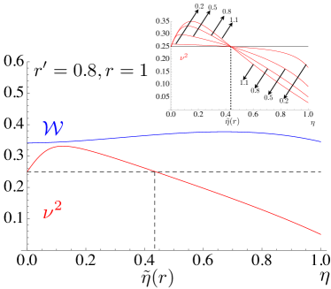
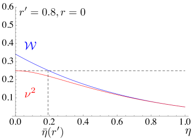
Figure 4: (Color online) Gaussian witness $\mathcal{W}$ (blue lines) and theoretical test $\nu^{2}$ (red lines) for the setup 1 of Fig. 2 ($r=1$, subfigure (a)) and for the setup 2 of Fig. 2 ($r=0$, subfigure (b)). In both cases the two-mode squeezing parameter of the initial state has been fixed to $r^{\prime}=0.8$. The inset of subfigure (a) shows instead the behavior of $\nu^{2}$ for different values of $r^{\prime}$. Here, one can verify that the EB threshold $\tilde{\eta}$ is independent from the initial entanglement as a consequence of the property introduced in Sec. I.2. However, larger values of $r^{\prime}$ allow for a clean-cut discrimination of the two regions.

Summarizing if we fix the squeezing parameter $r$, in order to get a reliable test by measuring $\mathcal{W}$ for both setups, the transmissivity $\eta$ of the beamsplitter should be fixed such that

$$\bar{\eta}(r^{\prime})\leq\eta\leq\tilde{\eta}(r)\,.$$ (49)

Under these conditions the witness measurement we have selected allows us to verify that $\rho_{\Phi_{2}}$ is entangled [meaning that $\Phi_{2}$ is not EB]. At the same time the state $\rho_{\Phi_{1}}$ will not pass the entanglement witness criterion in agreement with the fact that $\Phi_{1}$ is EB. Of course this last result can not be used as an experimental proof that $\Phi_{1}$ is EB since, to do so, we should first check that no other entanglement witness bound is violated by $\rho_{\Phi_{1}}$. Notice that this drawback can be avoided if we are able to compute the optimal witness $\nu^{2}$ by measuring the full covariance matrix of the output state. Finally, let us stress that $\tilde{\eta}(r)$ in the final relation (49) does not depend on the two-mode squeezing of the incoming twin-beam (see inset of Fig. 4 (a) ) and thus we do not need to test the EB properties of our maps on states characterized by an infinite amount of energy, that is on maximally-entangled states. This represents an important observation, especially from the point of view of the experimental implementation of our scheme. A more detailed analysis of possible experimental losses and detection errors will be addressed in a future work exp .

II.2 Example 2: asymmetric noise-phase shift-asymmetric noise

In the previous section we have seen a class of EB Gaussian channels which are amendable through a squeezing filtering transformation $\mathcal{S}(r)$. Here we focus on channels which are amendable with a different unitary filter: a phase shift $\mathcal{R}(\theta)$. According to the previous notation, the phase shift $\mathcal{R}(\theta)$ can be represented with the triplet:

$$K_{\mathcal{R}} = R(\theta)^{T}$$ (50)

$$l_{\mathcal{R}} = 0$$ (51)

$$\beta_{\mathcal{R}} = 0$$ (52)

where

$$R(\theta)=\begin{pmatrix}\cos(\theta)&\sin(\theta)\\ -\sin(\theta)&\cos(\theta)\,\end{pmatrix}$$ (53)

is a phase space rotation of an angle $\theta$.

Following the analogy with the previous case we look for a channel $\Phi$, such that the concatenation

$$\Phi\circ\mathcal{R}(\theta)\circ\Phi$$ (54)

is EB or not EB, depending on the value of $\theta$.

It is easy to check that $\Phi$ cannot be an attenuation channel because in this case it would simply commute with the filtering operation $\mathcal{R}(\theta)$. A good candidate is instead the channel $\Phi_{\mathcal{P}}(\eta,N_{\mathcal{P}})$, given by

$$K_{\mathcal{P}} = \sqrt{\eta}\openone$$ (55)

$$l_{\mathcal{P}} = 0$$ (56)

$$\beta_{\mathcal{P}} = N_{\mathcal{P}}\Pi+\frac{1-\eta}{2}\openone$$ (57)

where $\Pi=\left(\begin{array}[]{cc}0&0\\ 0&1\end{array}\right)$, $0\leq\eta\leq 1$ and $N_{\mathcal{P}}\geq 0$. Notice that this corresponds to an attenuation channel where the noise affects only the $P$ quadrature of the mode. This channel does not commute with a phase shift $\mathcal{R}(\theta)$ and, as we are going to show, the composition $\Phi_{\mathcal{PRP}}(\theta)=\Phi_{\mathcal{P}}\circ\mathcal{R}(\theta)\circ\Phi_{\mathcal{P}}$ is EB only for some values of the angle $\theta$.

From the composition law in Eq. (10) we have that the total map $\Phi_{\mathcal{PRP}}(\theta)$ is given by

$$K_{\mathcal{PRP}} = \eta R(\theta)$$ (58)

$$l_{\mathcal{PRP}} = 0$$ (59)

$$\beta_{\mathcal{PRP}} = N_{\mathcal{P}}\left(\eta R(\theta)\Pi R(\theta)^{T}+\Pi\right)+\frac{1-\eta^{2}}{2}\openone\,.$$ (60)

The entanglement breaking condition given in Eq. (11), is equivalent to $\nu^{2}\geq 1/4$ as explained in Sec. I.2. This implies that

$$\Phi_{\mathcal{PRP}}(\theta)\text{ is EB}\Longleftrightarrow\nu^{2}\geq\frac{1}{4}\Longleftrightarrow\theta_{min}\leq\theta\leq\theta_{max},$$ (61)

where $\theta_{min}$ and $\theta_{max}$ are solutions of the equation $\nu(\theta)^{2}=1/4$. They can be explicitly determined: $\theta_{min}=\text{arcos}(\sqrt{c})$ and $\theta_{max}=\text{arcos}(-\sqrt{c})$, where

$$c=\frac{2\eta N_{\mathcal{P}}^{2}-2\eta^{2}-(\eta-1)(\eta+1)^{2}N_{\mathcal{P}}}{2\eta N_{\mathcal{P}}^{2}}.$$ (62)

The two solutions make sense only in the cases in which $0\leq c\leq 1$. We may identify this as an amendability condition. Otherwise, in the cases in which there are no admissible solutions, it means that the channel is constantly EB or not EB independently of the filtering operation.

II.2.1 Experimental test

If we want to experimentally test the EB property of the channel $\Phi_{\mathcal{PRP}}(\theta)$ as a function of the filtering parameter $\theta$, we should be able to realize the operations $\Phi_{\mathcal{P}}(\eta,N_{\mathcal{P}})$ and $\mathcal{R}(\theta)$.

A phase shift operation $\mathcal{R}(\theta)$ applied to an optical mode can be realized by changing the effective optical path. This is a classical passive operation and it is experimentally very simple. The main difficulty is now the realization of the channel $\Phi_{\mathcal{P}}(\eta,N_{\mathcal{P}})$. A possible way to realize $\Phi_{\mathcal{P}}(\eta,N_{\mathcal{P}})$ is to combine a beam splitter with an additive phase noise channel $\mathcal{N}(N_{\mathcal{P}})$. This is defined by the triplet

$$K_{\mathcal{N}} = 0$$ (63)

$$l_{\mathcal{N}} = 0$$ (64)

$$\beta_{\mathcal{N}} = N_{\mathcal{P}}\Pi$$ (65)

and is it essentially a random displacement $W(\delta,0)$ of the $P$ quadrature, where the shift $\delta$ is drawn from a Gaussian distribution of variance $N_{\mathcal{P}}$ and mean equal to zero. This could be realized via an electro-optical phase modulator driven with classical electronic noise or by other techniques. It is immediate to check that $\Phi_{\mathcal{P}}(\eta,N_{\mathcal{P}})=\mathcal{N}(N_{\mathcal{P}})\circ\Phi_{\mathrm{At}}(\eta,0),$ i.e. a beam splitter followed by classical phase noise is a possible experimental realization of the channel $\Phi_{\mathcal{P}}(\eta,N_{\mathcal{P}})$.

The proposed experimental setup is sketched in Fig. 5.

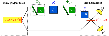
Figure 5: Schematic of the experimental proposal discussed in Sec. II.2. As in Fig. 2 the setup is divided in three stages (preparation of the probing state $|TMSV\rangle$, application of the channels, and finally measurement of the output state). The global map is obtained by applying twice the Gaussian channel $\Phi_{\mathcal{P}}$ with the intermediate insertion of a unitary phase shifter $\mathcal{R}(\theta)$. Depending on the value of the phase shift $\theta$ the global channel is EB or not.

A two-mode squeezed state is prepared and the desired sequence of channels is applied on one mode of the entangled pair. The presence of entanglement after the application of all the channels is verified by measuring the variances of $Q$ and $P$ defined in (22) after a unitary correction $\mathcal{R}(-\theta)$. This correction does not change the entanglement of the state but it is important for optimizing the entanglement criterion (21).

A possible experiment could be to measure the witness for various choices of the filtering operation, or in other words for various values of $\theta$. One should check that the condition for entanglement $\mathcal{W}<1/4$ is verified only for some angles $\theta$ while for $\theta_{min}\leq\theta\leq\theta_{max}$ we must have $\mathcal{W}\geq 1/4$ because the channel is EB. As a figure of merit for the quality of the experiment, the witness $\mathcal{W}$ can be compared with the corresponding optimal witness $\nu^{2}$.

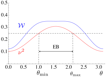
Figure 6: Entanglement witness $\mathcal{W}$ and optimal theoretical witness $\nu^{2}$ as functions of the angle $\theta$ for the setup of Fig. 5 with parameters: $r^{\prime}=2$, $\eta=0.9$ and $N_{\mathcal{P}}=1$. In this case we find that the global channel is entanglement breaking only in the region $\theta_{\mathrm{min}}<\theta<\theta_{\mathrm{max}}$ where, $\theta_{\mathrm{min}}=0.99$ and $\theta_{max}=2.15$.

The results are plotted in Fig. 6. For some values of $\theta$, one can experimentally show that the channel is not EB. On the other hand, inside the entanglement breaking region, the witness is consistently larger than $1/4$. Again, we underline that, if we are able to measure the covariance matrix of the output state, the product criterion can be replaced by the optimal one $\nu^{2}<1/4$ (see Eq. (26)).

As a final remark we stress that, even though it is realistic to consider $\eta<1$ to account for experimental losses, the same qualitative results are possible in the limit of $\eta=1$, i.e. without the two beam splitters. In this case the amendability condition $0\leq c\leq 1$ (see Eq. (62)) implies $N_{\mathcal{P}}\geq 1$ and the global map is EB for

$$\arccos\left(\sqrt{1-1/N^{2}_{\mathcal{P}}}\right)\leq\theta\leq\arccos\left(-\sqrt{1-1/N^{2}_{\mathcal{P}}}\right).$$

Conclusions

In this paper we proved the existence of amendable Gaussian maps by constructing two explicit examples. For each of them we put forward an experimental proposal allowing the implementation of the map. We took as benchmark model the set of entanglement breaking maps, and presented a sort of “error correction” technique for Gaussian channels. Differently from the standard encoding and decoding procedures applied before and after the action of the map nogo , it consists in considering a composite map $\Phi\circ\Phi$ with $\Phi\in{\mathrm{EB}}^{2}$ and applying a unitary filter between the two actions of the channel so as to prevent the global map from being entanglement breaking.

We focused on two-mode Gaussian systems. We recall that in order to test the entanglement breaking properties of a map we have to apply it, tensored with the identity, to a maximally-entangled state, which in a continuous variable setting would require an infinite amount of energy. However in Sec. I.2 we have proved that without loss of generality it is sufficient to consider a two-mode squeezed state with finite entanglement. This property is crucial for the experimental feasibility of our schemes. Finally, in order to verify if the entanglement of the input state survives after the action our Gaussian maps, we applied the product criterion to the out coming modes prodcrit , and compared it with the entanglement-negativity. The latter analysis enabled us to properly set the intervals to which the experimental parameters have to belong in oder to consider the product criterion reliable.

This analysis paves the way to a broad range of future perspectives. One possibility would be to extend it to the case of multimode Gaussian or non Gaussian maps. Another compelling isuee would be determining a complete characterization of amendable Gaussian maps of second or higher order. We recall that, according to the definition introduced in mucritico , a map $\Phi$ is amendable of order $m\geq 2$, if $\Phi\in{\mathrm{EB}}^{2}$ and it is possible to delay its detrimental effect by $m-2$ steps by applying the same intermediate unitary filter after successive applications of the channel. One possible outlook in this direction would be to allow the choice of different filters at each error correction step and determine an optimization procedure over the filtering maps. Of course this analysis would be extremely difficult to be performed for arbitrary noisy maps. A first step would be to focus on set of the Gaussian maps using the conservation of the Gaussian character under combinations among them and their very simple composition rules to perform this analysis.

References

- (1) M. Horodecki, P. W. Shor, M. B. Ruskai, Rev. Math. Phys 15, 629 (2003);
- (2) A. S. Holevo, Russian. Math. Surveys 53, 1295 (1999);
- (3) S. L. Braunstein and P. van Loock, Rev. Mod. Phys. 77, 513 (2005); C. Weedbrook, S. Pirandola, R. Garcia-Patron, N. J. Cerf, T. C. Ralph, J. H. Shapiro and S. Lloyd, Rev. Mod. Phys. 84, 621 (2012);
- (4) A. S. Holevo and R. F. Werner, Phys. Rev. A 63 032312 (2001); A. Ferraro, S. Olivares and M. G. A. Paris, Gaussian states in continuous variable quantum information, (Bibliopolis, Napoli) (2005); J. Eisert and M. M. Wolf, Gaussian quantum channels in Quantum Information with Continous Variables of Atoms and Light, 23 (Imperial College Press, London) (2007); F. Caruso, J. Eisert, V. Giovannetti and A. S. Holevo, Phys. Rev. A 84, 022306 (2011);
- (5) A. S. Holevo and V. Giovannetti, Rep. Prog. Phys. 75, 046001 (2012);
- (6) A. S. Holevo, Problems of Information Transmission 44, 3 (2008); A. S. Holevo, M. E. Shirokov and R. F. Werner, Russ. Math. Surv. 60, 359 (2005);
- (7) D. Buono, G. Nocerino, A. Porzio, and S. Solimeno, Phys. Rev. A 86, 042308 (2012);
- (8) J. Niset, J. Fiurášek and N. J. Cerf, Phys. Rev. Lett. 102, 120501 (2009);
- (9) A. De Pasquale and V. Giovannetti, Phys. Rev. A 86, 052302 (2012);
- (10) A. S. Holevo, J. Math. Phys. 52, 042202 (2011);
- (11) M.D. Reid, Phys. Rev. A 40, 913 (1989); V. Giovannetti, S. Mancini, D. Vitali, and P. Tombesi, Phys. Rev. A 67, 022320 (2003);
- (12) A. Peres, Phys. Rev. Lett. 77, 1413 (1996); P. Horodecki, M. Horodecki and R. Horodecki J. Mod. Opt. 47 347 (2000); R. Simon, Phys. Rev. Lett. 84, 2726 (2000);
- (13) W. P. Bowen, R. Schnabel, P. K. Lam, and T. C. Ralph Phys. Rev. A 69, 012304 (2004); J. Laurat, G. Keller, J. A. Oliveira-Huguenin, C. Fabre, T. Coudreau, A. Serafini, G. Adesso, and F. Illuminati, J. Opt. B: Quantum Semiclass. Opt. 7, S577 (2005);
- (14) Virginia D’Auria, Alberto Porzio, Salvatore Solimeno, Stefano Olivares, and Matteo G A Paris, J. Opt. B: Quantum Semiclass. Opt. 7, S750 (2005);
- (15) A. De Pasquale, A. Mari, V. Giovannetti, D. Buono, G. Nocerino and A. Porzio, in preparation.