Spatial distribution of small hydrocarbons in the neighborhood of the Ultra Compact HII region Monoceros R2^,

Abstract

Context. We study the chemistry of small hydrocarbons in the photon-dominated regions (PDRs) associated with the ultra-compact H ii region (UCH ii) Mon R2.

Aims. Our goal is to determine the variations of the abundance of small hydrocarbons in a high-UV irradiated PDR and investigate the chemistry of these species.

Methods. We present an observational study of the small hydrocarbons CH, CCH and c-C₃H₂ in Mon R2 combining spectral mapping data obtained with the IRAM-30m telescope and the Herschel space observatory. We determine the column densities of these species, and compare their spatial distributions with that of polycyclic aromatic hydrocarbon (PAH), which trace the PDR. We compare the observational results with different chemical models to explore the relative importance of gas-phase, grain-surface and time-dependent chemistry in these environments.

Results. The emission of the small hydrocarbons show different spatial patterns. The CCH emission is extended while CH and c-C₃H₂ are concentrated towards the more illuminated layers of the PDR. The ratio of the column densities of c-C₃H₂ and CCH shows spatial variations up to a factor of a few, increasing from $N(\mbox{c-C${}_{3}$H${}_{2}$})/N(\mbox{CCH})\approx 0.004$ in the envelope to a maximum of $\approx 0.015-0.029$ towards the 8 $\mu$m emission peak. Comparing these results with other galactic PDRs, we find that the abundance of CCH is quite constant over a wide range of $G_{\rm 0}$, whereas the abundance of c-C₃H₂ is higher in low-UV PDRs, with the $N(\mbox{c-C${}_{3}$H${}_{2}$})/N(\mbox{CCH})$ ratio ranging $\approx$0.008-0.08 from high to low UV PDRs. In Mon R2, the gas-phase steady-state chemistry can account relatively well for the abundances of CH and CCH in the most exposed layers of the PDR, but falls short by a factor of 10 to reproduce c-C₃H₂. In the low-density molecular envelope, time-dependent effects and grain surface chemistry play a dominant role in determining the hydrocarbons abundances.

Conclusions. Our study shows that the small hydrocarbons CCH and c-C₃H₂ present a complex chemistry in which UV photons, grain-surface chemistry and time dependent effects contribute to determine their abundances. Each of these effects may be dominant depending on the local physical conditions, and the superposition of different regions along the line of sight leads to the variety of measured abundances.

1 Introduction

Ultracompact H ii regions (UCH ii) represent one of the earliest phases in the formation of a massive star. In these environments, the chemistry is strongly driven by the mutual interaction between the gas, the dust and the UV photons from nearby stars. The H-ionizing photons are absorbed in a thin layer around the star, forming the H ii region, while the UV radiation carrying energies less than 13.6 eV penetrate in the deeper layers of the molecular cloud and produce the so-called photon-dominated region (PDR). In these environments, the thermal balance, the chemistry and ionization balance are driven by UV photons. PDRs associated with UCH ii are characterized by extreme UV field intensities (expressed in units of the Habing field $G_{\rm 0}$, see Habing, 1968) and small physical scales ($\lesssim 0.1$ pc). These environments are therefore ideal to study the effect of a strong UV field on the chemistry of gas-phase species.

The chemistry of small hydrocarbons in PDRs is still poorly constrained. The comparison of observations and gas-phase chemical models showed that this type of chemistry alone cannot account for the abundance of small hydrocarbons, especially for those species containing more than two C atoms: in NGC 7023, the Orion Bar (Fuente et al., 2003), IC63 and the Horsehead nebula (Teyssier et al., 2004) the abundances of species such as c-C₃H₂ and C₄H derived from the observations are at least an order of magnitude larger compared to model predictions. This discrepancy was confirmed by high spatial resolution observations and detailed modeling of the Horsehead nebula (Pety, 2005), in which the emission of small hydrocarbons was compared to other PDR tracers such as the mid-IR emission in the aromatic infrared bands (AIBs) due to polycyclic aromatic hydrocarbons (PAHs). The authors suggested that small hydrocarbons may form through non gas-phase processes such as the photo-destruction of the AIB carriers. In the Horsehead (Pety, 2005) and in NGC 7023 (Pilleri et al., in prep.), the spatial distributions of CCH and c-C₃H₂  are strikingly similar. Similarly, a tight correlation between these two hydrocarbons has been observed by Lucas & Liszt (2000) and Gerin et al. (2011) on several lines of sights in the diffuse medium. The small radical CH has also a relatively constant abundance in these environments (Sheffer et al., 2008). In low- to mild-UV irradiated PDRs ($G_{\rm 0}\sim 100$ for the Horsehead and $\sim 2600$ for NGC7023) the tight correlation between CCH and c-C₃H₂ suggests a common origin of these two small hydrocarbons. However, this spatial correlation has not been explored yet in highly UV-illuminated PDRs ($G_{\rm 0}\gtrsim 1\times 10^{4}$).

In this paper, we present new observations of several lines of CH, CCH and c-C₃H₂ in the PDRs associated with the UCH ii region Mon R2 and investigate observationally the relative variations of these species. In Sect. 2 we present the source and the observations, and the results are reported in Sect. 3. In Sect. 4 we calculate column densities and abundances, while in Sect. 5 we compare the spatial distributions to that of other PDR tracers and discuss the quantitative consistence with different chemical models. Finally, Sect. 6 presents the conclusions and perspectives.

2 Observations

2.1 Mon R2

Mon R2 is a close-by ultracompact H ii region (d=830 pc), which comprises several PDRs that can be spatially resolved in both the mm and IR domains. Due to its brightness and proximity, this source can be used as reference for other PDRs illuminated by a strong UV field. The most intense UV source is called IRS1 and it is located at the center of the UCH ii (see Fig.1). A low-density molecular cloud surrounds this innermost region and extends for several arcminutes. The brightest PDR of Mon R2, which surrounds the UCH ii and peaks at about 20″  to the NW of IRS1, shows both very intense AIB emission and H₂ rotational lines (Berné et al., 2009) and is due to the illumination of the internal walls of the molecular cloud by IRS1. This PDR is very compact ($d\sim 5\arcsec$) and illuminated by a very strong radiation field ($G_{\rm 0}\sim 5\times 10^{5}$). A secondary PDR, detected north of the UCH ii at a distance of about 1′ from IRS1, is much fainter and more extended. The northern Molecular Peak position at [0″ ;40″] (hereafter MP2 following the nomenclature of Ginard et al., 2012) is clearly detected in the AIB emission at 8$\,\mathrm{\mu m}$, and its chemical properties seem to be similar to those of low- to mild-UV irradiated PDRs (Ginard et al., 2012). The origin of this PDR could be the outer envelope of the molecular cloud illuminated by an external UV field, or it could be due to UV photons that are escaping from IRS1 through a hole, illuminating its walls.

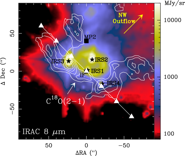
Figure 1: Overview of the region. The color image displays the IRAC 8$\,\mathrm{\mu m}$ emission (Ginard et al., 2012), in which both the bright circular PDR and the extended northern PDR can be distinguished beneath the peaks due to the young stellar objects. The white contours represent the integrated intensity of the C¹⁸O (2$\rightarrow$1) line between 5 and 15 $\,\mathrm{km\,s^{-1}}$ observed at the IRAM 30m telescope (Pilleri et al., 2012a), with contour levels from 16 to 24$\,\mathrm{K}$ $\,\mathrm{km\,s^{-1}}$ in linear steps of 2$\,\mathrm{K\,km\,s^{-1}}$. The black squares represent the positions of the ionization front (IF) and the molecular peak (MP2), whereas the triangles and the white line indicate the positions observed with HIFI. The black stars indicate the position of the most intense infrared sources following the nomenclature of Henning et al. (1992). The yellow arrow indicates the direction of the NW molecular outflow (Tafalla et al., 1994).

Although there are some asymmetries in the general shape of the cloud, such as the molecular hole to the NW, we can assume as a zero-order approximation that the dense core around the UCH ii region is spherical and composed by concentric shells centered on IRS1, a simplified model which is close to reality in most outwards directions. Each of the shells has its own physical conditions (kinetic temperature, gas density, $G_{\rm 0}$) which vary with radius. In the following, we will assume the physical parameters presented in Pilleri et al. (2012a) and schematized in Fig. 2: the region immediately surrounding the star is an H ii region, which is expanding at a velocity of $\sim 10$$\,\mathrm{km\,s^{-1}}$ (Choi et al., 2000) and which is free of any molecular gas. The diameter of the region is $\sim 40$″, corresponding to $\sim 0.08$ pc. This is followed by a thin (1 mag), high UV-irradiated PDR, which has a density of $n_{\mathrm{H_{2}}}\sim 2\times 10^{5}$$\,\mathrm{cm^{-3}}$ and a gas kinetic temperature of $\sim 100$$\,\mathrm{K}$ (Berné et al., 2009). Going farther from IRS1, there is a thicker ($\sim 8\leavevmode\nobreak\$mag), warm ($T_{\mathrm{kin}}\sim 70$$\,\mathrm{K}$) and high density ($n_{\mathrm{H_{2}}}$ $\sim 3\times 10^{6}$$\,\mathrm{cm^{-3}}$, Rizzo et al., 2003) PDR, which is expanding at a velocity of $\lesssim 1$$\,\mathrm{km\,s^{-1}}$ (Fuente et al., 2010; Pilleri et al., 2012a). This high-density layer is surrounded by the parent molecular cloud, which is about 40 mag thick, has a relatively low density ($n_{\mathrm{H_{2}}}$ $\sim 5\times 10^{4}$$\,\mathrm{cm^{-3}}$) and temperature ($T_{\mathrm{kin}}$ $\sim 35\,\mathrm{K}$), and is rather quiescent (Fuente et al., 2010; Pilleri et al., 2012a). The cloud is also illuminated from the outside with a UV field of $G_{\rm 0}\sim 100$.

The presence of these different phases and its proximity make Mon R2 the best source to investigate the chemistry and physics of these extreme PDRs and their parent molecular clouds.

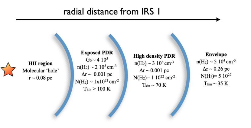
Figure 2: A 1D schematic of the geometry of MonR2 as a function of the radial distance to IRS1.

Table 1: Summary of the observations

Line(s)	Frequency	Instrument	FWHM	$\eta_{l}$	Position	OM	$T_{\rm{rms}}$
	[$\,\mathrm{GHz}$ ]		[”]				[$\,\mathrm{K}$ ]
C18O $J=2-1$	219.560	IRAM-HERA	10.0	0.67	Map	OTF	0.025
C18O $J=5-4$	548.830	Herschel-HIFI	38.6	0.79	Strip	OTF	0.008
CH $J=3/2-1/2$	536.761	Herschel-HIFI	38	0.77	Strip	OTF	0.041
CH $J=5/2-3/2$	1656.961	Herschel-HIFI	12.8	0.74	IF	SP	0.284
CCH $N=1-0$	87.317	IRAM	29	0.85	Map	OTF	0.070
CCH $N=3-2$	262.004	IRAM-HERA	9	0.6	Map	OTF	0.380
CCH $N=6-5$	523.972	Herschel-HIFI	40.5	0.78	Strip	OTF	0.057
c-C3H2 $J_{K_{A},K_{C}}=2_{1,2}-1_{0,1}$	85.33889	IRAM	29	0.85	Map	OTF	0.070
c-C3H2 $J_{K_{A},K_{C}}=4_{0,4}-3_{1,3}$	150.82067	IRAM	16	0.64	Map	OTF	0.054
c-C3H2 $J_{K_{A},K_{C}}=4_{1,4}-3_{0,3}$	150.85191	IRAM	16	0.64	Map	OTF	0.054
c-C3H2 $J_{K_{A},K_{C}}=6_{1,6}-5_{0,5}$	217.82215	IRAM-HERA	11	0.61	Map	OTF	0.016
c-C3H2 $J_{K_{A},K_{C}}=5_{1,4}-4_{2,3}$	217.94005	IRAM	11	0.61	Map	OTF	0.150
c-C3H2 $J_{K_{A},K_{C}}=4_{3,2}-4_{2,1}$	227.16913	IRAM	10	0.59	Map	OTF	0.150
c-C3H2 $J_{K_{A},K_{C}}=7_{0,7}-6_{1,6}$	251.31434	IRAM	9	0.55	Map	OTF	0.115
c-C3H2 $J_{K_{A},K_{C}}=6_{2,5}-5_{1,6}$	251.52730	IRAM	9	0.55	Map	OTF	0.115

.

2.2 IRAM and Herschel observations

We observed several low-lying rotational transitions of CCH and c-C₃H₂ at mm wavelengths using the IRAM-30m telescope. We completed this dataset with Herschel (Pilbratt et al., 2010) observations of a higher excitation line of CCH and two lines of CH. A summary of the spectroscopic parameters for all the observed lines are given in Table 7. Throughout the paper, we will use main beam temperature as intensity scale. Offset positions are given relative to the ionization front (IF: $\alpha_{J2000}$=06h07m46.2s, $\delta_{J2000}=-06^{\circ}23^{\prime}08.3^{\prime\prime}$). For all the observations, the OFF position was chosen to be free of molecular emission ([+10′,0′] for Herschel; [+400″, -400″] for IRAM). A summary of the observations is shown in Table 1.

The 3mm and 2mm observations were performed in July 2012 at the IRAM-30m telescope in Pico Veleta (Spain). We observed the CCH multiplet at 87$\,\mathrm{GHz}$ and the c-C₃H₂ line at 85$\,\mathrm{GHz}$ using the EMIR receivers with the VESPA correlators, covering a 180″$\times$180″  region centered toward the IF. The 1 mm observations were performed in two different sessions using the HERA 3x3 dual-polarisation receiver and in a successive run with the EMIR receivers. During the first run (HERA) we obtained a 150″$\times$150″ map of the CCH multiplet at 262$\,\mathrm{GHz}$ and the c-C₃H₂ line at 217$\,\mathrm{GHz}$. The second observing run (January 2012) was part of a 2-D spectral survey at 1mm (Treviño-Morales, et al., 2012, in prep.). The resulting c-C₃H₂ maps have a lower signal-to-noise ratio (SNR) and the field of view covered in this second run was smaller, 2′$\times$2′.

The Herschel observations were obtained with the Heterodyne Instrument for the Far Infrared (HIFI, de Graauw et al., 2010) in the context of the WADI guaranteed-time key program (Ossenkopf et al., 2011). The CH lines were observed with both the wide band spectrometer (WBS) and the high-resolution spectrometer (HRS). They provide spectral resolutions (at 500$\,\mathrm{GHz}$) of $\Delta{\rm v}$ = 1.2$\,\mathrm{km\,s^{-1}}$ and 0.3$\,\mathrm{km\,s^{-1}}$, respectively, allowing to resolve the line profiles. Cross-calibration between the two backends and between the two polarizations indicates an uncertainty of $\sim 20\%$. The CH (J = 3/2-1/2) and CCH (N=6-5) observations were performed in on-the-fly (OTF) observing mode along the strip indicated in Fig. 1 while the excited ($J=5/2-3/2$) line of CH was observed in single pointing observing mode towards the IF, with a double beam switching pattern. In this paper we also compare the new observations with the [C ii ] strip already presented by Pilleri et al. (2012a).

2.3 Data reduction

The basic data reduction of Herschel observations was performed using the standard pipeline provided with the version 7.0 of HIPE (Ott, 2010) and Level 2 data were exported to the FITS format. The Herschel and IRAM-30m data were then processed using the GILDAS/CLASS software suite (Pety, 2005). The spectra were first calibrated to the $T_{\mathrm{A}}^{*}$ scale using the chopper wheel method (Penzias & Burrus, 1973), and finally converted to the main beam temperatures ($T_{\mathrm{mb}}$) using the nominal forward ($F_{\mathrm{eff}}$) and main beam ($B_{\mathrm{eff}}$) efficiencies (in Table 1, we show the value $\eta_{l}={B_{\mathrm{eff}}/F_{\mathrm{eff}}}$). The HIFI efficiencies have been recently calculated by Roelfsema et al. (2012). The resulting amplitude accuracy is $\sim$ 10% for both HIFI and IRAM observations.

Visual inspection of the IRAM data revealed for all the observed lines 1) the presence of more or less pronounced spikes at one quarter and three quarter of the correlator window, 2) the presence of platforming in the middle of the correlator window, 3) but otherwise clean baselines. Windows around the well-defined frequencies displaying spikes were set before baselining. The line windows were defined on the spectra averaged over the map, from [-1,24.5$\,\mathrm{km\,s^{-1}}$ ] for the brightest lines to [6,16$\,\mathrm{km\,s^{-1}}$ ] for the faintest ones. To correct for the platforming, a zero-order baseline was subtracted from each correlator sub-bands of each spectrum. A first-order baseline was needed for c-C₃H₂. The bad channels, which occurred in a line-free section of the HERA spectra, were replaced by Gaussian noise of same rms. The resulting spectra were resampled and convolved with a Gaussian to a map resolution larger than the HPBW of the telescope. The map resolution is reported in Table 1. The spectral cubes were finally blanked where the spectra weights (resulting from the gridding) were too low, giving the fringed aspect of the map edges.

3 Results

In this section, we describe the spectral and spatial variations of the various molecular tracers. First, we present all the observations obtained towards the IF, which is one of the best-known position (see, for instance, Fuente et al., 2010; Ginard et al., 2012; Pilleri et al., 2012a). We then describe the spatial/spectral variations along the Herschel strip (see Fig. 1) and finally, we present the full maps.

3.1 The ionization front

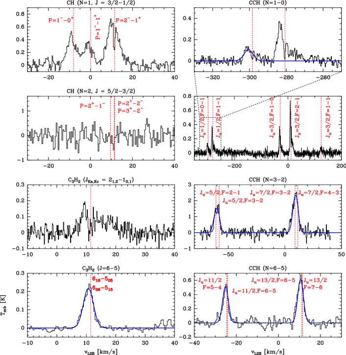
Figure 3: Herschel and IRAM observations of CCH and c-C₃H₂ towards the IF. 1mm observations have been convolved to the spatial resolution of 39″. Solid blue lines show the single-component Gaussian fits. The velocity scale in each panel is relative to the most intense line in the hyperfine groups (see also Tables 1 and 7).

In Fig. 3 we show the spectra of several CH, CCH and c-C₃H₂ transitions observed towards the IF with the IRAM-30m and Herschel. The lower-lying transitions show a self-absorption feature at the ambient velocity of the cloud ($\sim 11$$\,\mathrm{km\,s^{-1}}$). It is clearly detected in the main hyperfine components of CH, CCH and c-C₃H₂, and coincides with the self-absorption detected in the [C ii ] strip observed with Herschel (Pilleri et al., 2012a). The self-absorption is barely visible in the faintest hyperfine components of the CCH 1-0 line and is not detected in any of the higher energy transitions. The structure of the CCH 3-2 line is due to the superposition of two hyperfine transitions with very similar frequencies that are not self-absorbed. The lower-lying transitions show some emission in the red and blue wings, which may trace either an expanding PDR (Pilleri et al., 2012a) or the molecular outflow (Tafalla et al., 1997).

3.2 The NE-SW strip

CH and C¹⁸O (5-4) have been observed only towards the NE-SW strip shown in Fig. 1. This strip, already studied in Pilleri et al. (2012a), passes through the IF and extend up to 1.5′ in each direction, crossing the main PDRs of the region and extending to offsets where the emission is dominated by the molecular envelope. However, the large beam of Herschel at this frequency ($\sim 40$″) results in even the positions [$\pm 40\arcsec,\pm 40\arcsec$] picking-up some emission from the innermost PDR.

In Fig. 4 we show the position-velocity (PV) diagrams along the cut observed with Herschel, i.e. in the direction perpendicular to the molecular outflow (Tafalla et al., 1994, 1997), which extends in the northwest-southeast direction from the IF. For a comparison, we also display the PV diagram of the [C ii ] line along the same cut (Pilleri et al., 2012a). For each transition, we show the diagram of the component with the highest signal-to-noise ratio (SNR). Although the data have very different angular resolutions, the spatial variation of CH is in some way similar to that of [C ii ]: for instance, in both tracers the emission is extended up to 60″  from the IF and the main component shows self-absorption through the whole cut. Both lines present a secondary peak at a distance of $\sim 10\arcsec$ at about 8$\,\mathrm{km\,s^{-1}}$. The line widths are also similar indicating that the CH emission, like [C ii ], originates in the innermost layers of the expanding central PDR.

The PV diagram of CCH 1-0 is very similar to the C¹⁸O 2-1 line in terms of the spatial extension and line width. They are both detected along the entire strip, and their typical line width is about 2.5$\,\mathrm{km\,s^{-1}}$. However, the CCH line toward the IF displays self-absorption at central velocities and emission in the red wing. Similarly to the CCH 1-0 line, the c-C₃H₂ $2_{1,2}-1_{0,1}$ transition shows self-absorption at 11$\,\mathrm{km\,s^{-1}}$ and emission in the red wing toward the IF. However, it is less spatially extended and therefore likely associated with the innermost layers of the PDR. The higher-energy transitions of all species are less spatially extended compared to [C ii ] and CH and do not show self-absorption. Finally, there is a systematic shift of the peak velocity of about 2$\,\mathrm{km\,s^{-1}}$ going from the south-west towards the north-east of the IF, which has been attributed to either an asymmetry in the expansion pattern or to a large-scale slow rotation of the entire cloud (Loren, 1977; Pilleri et al., 2012a).

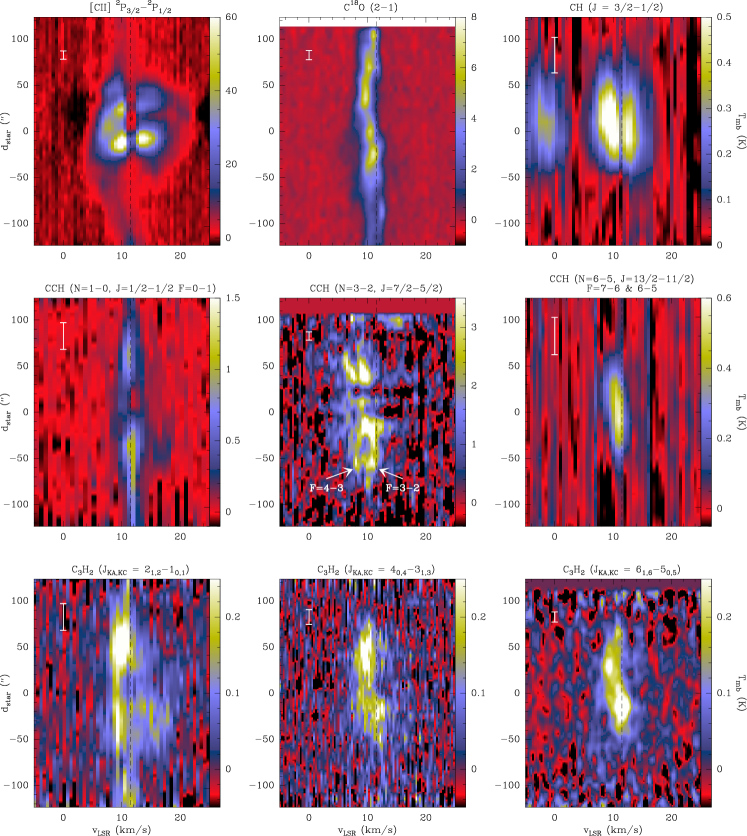
Figure 4: PV diagrams of the Herschel and IRAM observations along the SW-NE strip. The C ii diagrams comes from Pilleri et al. (2012a). The double peaked structure of the CCH lines is due to two hyperfine component of the same line, while the strong dip in both CH and [C ii ] are partially due to self-absorption. The white line in the top-right corner of each diagram represents the HPBW of the observation. The black dotted line indicates $v_{LSR}=11.5\,\mathrm{km\,s^{-1}}$.

3.3 Maps

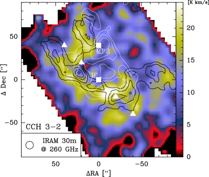
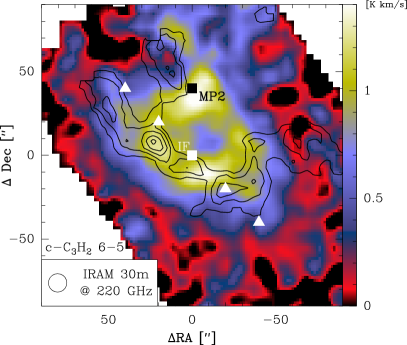
Figure 5: Maps of integrated intensity (in the range 5-15 $\,\mathrm{km\,s^{-1}}$) for CCH (262.004$\,\mathrm{GHz}$) and c-C₃H₂ (217.822$\,\mathrm{GHz}$) obtained with the EMIR receivers. Black contours are the C¹⁸O line shown in Fig. 1. White triangles and squares represent the single positions studied in this paper. White contours in the left panel represent the c-C₃H₂ line integrated intensities (in the range 5-15$\,\mathrm{km\,s^{-1}}$) starting from 0.6$\,\mathrm{km\,s^{-1}}$ and in linear steps of 0.2$\,\mathrm{km\,s^{-1}}$.

The maps carried out with the 30m telescope allow us to investigate about the spatial distribution of CCH and c-C₃H₂. Figure 5 shows the spatial distribution of the integrated line intensity of the CCH 3-2 and c-C₃H₂ 6-5 lines between 5 and 15$\,\mathrm{km\,s^{-1}}$ observed with HERA at the spatial resolution of 10″. The spatial pattern of CCH is very similar to that of C¹⁸O 2-1 (Fig. 1): the emission to the northeast and southwest extends up to 1′  from the IF, and peaks at a distance of $\sim 30\arcsec$. The emission is opened to the north and the northwest, following the cometary shape of the molecular bar. The c-C₃H₂ emission is more compact, with the center at an offset [-10″, +10″] relative to the IF. The emission extends less than 40″  from the center, and peaks at a distance of about 10″  south from the IF. The line intensity also displays a peak toward the MP2 position, which does not have a correspondence in the CCH map. The emission to the north is more extended compared to CCH, following the IRAC 8$\,\mathrm{\mu m}$ emission (Ginard et al., 2012).

4 Column densities and abundances

In this section, we derive the column densities and abundances of CH, CCH and c-C₃H₂. First, we concentrate in the SW-NE strip, where we use the Herschel observations to study CH and the excitation of C¹⁸O. We study in more details the excitation of CCH using a two-phase LVG model towards the IF and study the emission in the line wings. Finally, we extrapolate these results to the analysis of the full maps to obtain more information on the spatial distribution of these tracers. The self-absorption features are discussed in Appendix A.

4.1 The SW-NE strip

Table 2: Integrated intensity (using $T_{\mathrm{mb}}$ scale) between 5 and 15 $\,\mathrm{km\,s^{-1}}$, after smoothing the data to the larger $HPBW$ (40″  for CCH and C¹⁸O, 28″  for c-C₃H₂). Non-detections are given at a 3$\sigma$ level assuming a line width of 1$\,\mathrm{km\,s^{-1}}$. See Table 7 for the spectroscopic parameters.

	IF [0″; 0″]	[20″; 20″]	[40″; 40″]	[-20″; -20″]	[-40″; -40″]	MP2 [0″; 40″]
Transition	Area	Area	Area	Area	Area	Area
	[$\,\mathrm{K}$ $\,\mathrm{km\,s^{-1}}$ ]	[$\,\mathrm{K}$ $\,\mathrm{km\,s^{-1}}$ ]	[$\,\mathrm{K}$ $\,\mathrm{km\,s^{-1}}$ ]	[$\,\mathrm{K}$ $\,\mathrm{km\,s^{-1}}$ ]	[$\,\mathrm{K}$ $\,\mathrm{km\,s^{-1}}$ ]	[$\,\mathrm{K}$ $\,\mathrm{km\,s^{-1}}$ ]
C18O 2-1	14.56	15.55	15.71	15.68	13.12	13.90
C18O 5-4	13.04	13.38	13.26	12.12	11.03	-
CH ${}_{J=3/2-1/2,P=1^{-}-0^{+}}$ [5-12]	1.81	1.43	0.62	1.03	0.22	-
CH ${}_{J=3/2-1/2,P=2^{-}-1^{+}}$ [12-15]	1.19	0.74	0.36	0.95	0.22	-
CH J=5/2-3/2	$\lesssim 0.84$	-	-	-	-	-
CCH ${}_{N=1-0,\,F=0-1}$	0.98	1.35	1.39	1.61	1.87	1.29
CCH ${}_{N=3-2,\,J_{u}=5/2,F=4-3\,\&\,F=3-2}$	13.75	13.85	11.70	15.63	11.99	12.19
CCH ${}_{N=6-5,\,J_{u}=13/2,F=7-6\,\&\,F=6-5}$	4.97	4.97	4.05	5.02	3.73	-
c-C3H2 212	0.73	1.55	1.71	1.73	1.32	1.71
c-C3H2 404	0.45	0.44	0.44	0.45	0.19	0.67
c-C3H2 414	1.42	1.71	1.34	1.52	0.80	2.0
c-C3H2 432	0.63	0.46	0.37	0.49	0.32	0.53
c-C3H2 514	0.76	0.56	0.33	0.46	0.20	0.87
c-C3H2 ${}_{616\,\&\,606}$	0.99	1.00	0.52	0.85	0.42	1.01
c-C3H2 625	0.57	$<0.3$	$<0.3$	$<0.3$	$<0.3$	0.41
c-C3H2 ${}_{707\,\&\,717}$	0.69	0.61	$<0.4$	0.58	$<0.3$	0.78

C¹⁸O

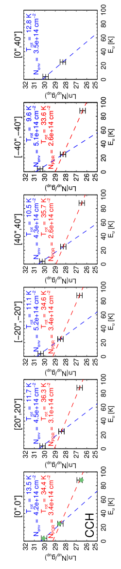
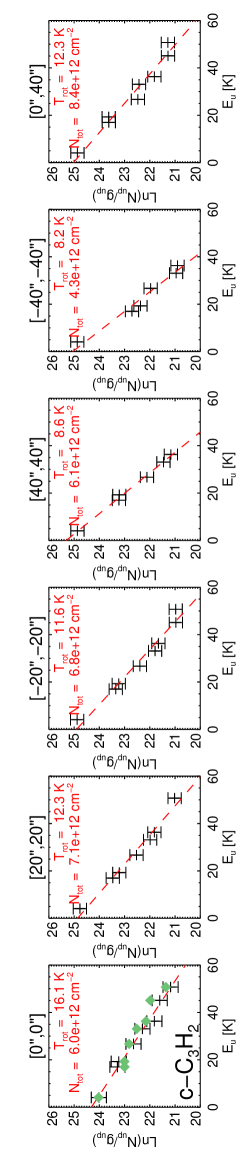
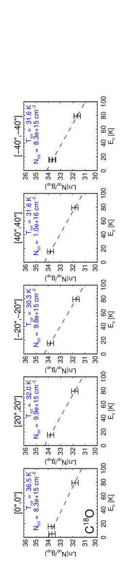
Figure 11: Rotational diagrams for CCH (top), c-C₃H₂ (middle) and C¹⁸O (bottom) along the Herschel strip. Data have been convolved to 40″  for CCH and C¹⁸O, and to 29″  for c-C₃H₂. Green diamonds represent the MADEX simulation towards the IF (cf. Sect. 4.2)

To obtain an estimate of the excitation temperature and column density of C¹⁸O along the Herschel strip, we have combined our J=2-1 observation with the J = 5-4 observations published in Pilleri et al. (2012a) and with the J = 1-0 observations of Ginard et al. (2012). We have convolved the data to the lowest spatial resolution (40″  for the J = 5-4) and built rotational diagrams for the five positions along the strip. The J=1-0 data cannot be convolved, since they were single pointing observations, but the spatial resolutions are not very different (29″  vs 40″) and the C¹⁸O emission is very extended, so that the emission fills the beam at both spatial resolutions. The corresponding rotational diagrams are shown in Fig.11. The results are consistent with those of Ginard et al. (2012): the rotation temperature slightly decreases from $\sim 37$$\,\mathrm{K}$ toward the IF to $\sim 31$$\,\mathrm{K}$ at a distance of 50″. We obtain a column density of $8.3\times 10^{15}$ $\,\mathrm{cm^{-2}}$ toward the IF, and slightly (20%) higher values at larger offsets. These values are consistent within a factor of 2 with the geometrical model presented by Pilleri et al. (2012a) to fit the high-J lines of CO, ¹³CO and C¹⁸O. This model consists of a spherical cloud with an $A_{V}=8$ PDR and an $A_{V}=40$ low-density envelope. This geometrical model yields a factor of 2 higher column densities compared to the C¹⁸O values, assuming an isotopic ratio ¹⁶O/¹⁸O = 500 and a standard abundance of CO relative to H₂ of $1\times 10^{-4}$. In the following, we assume therefore an uncertainty of a factor of 2 in the column density of H₂ and in the abundances of the hydrocarbons. However, the absolute value of the column densities, and consequently the relative abundances, are not affected by this uncertainty.

CH

As shown in Fig. 3, the main component of CH is self-absorbed at the ambient cloud velocity and the line wings of the different components overlap. To obtain the integrated intensity of the CH line, we used the $P=1^{-}-0^{+}$ and the $P=2^{-}-1^{+}$ transitions for the velocity intervals [5-12]$\,\mathrm{km\,s^{-1}}$ and [12-15]$\,\mathrm{km\,s^{-1}}$, respectively. Using the first satellite to obtain the area in the blue interval we avoid the self-absorption that affects the main component. On the other hand, the red part of the $P=1^{-}-0^{+}$ line is contaminated by the overlap with the second satellite, so that for this interval we have to rely on the main component. The integrated areas for each interval are shown in Table 2.

When computing the CH column density, we face the difficulty that there are no collisional rates available for CH, so that one can only assume a given rotational temperature $T_{\mathrm{rot}}$ per velocity interval. The non-detection of the CH triplet at 1656 GHz provides an upper limit to $T_{\mathrm{rot}}$ if we assume LTE conditions, so that both transitions share the same rotation temperature. This gives upper limits for $T_{\mathrm{rot}}$ of 25$\,\mathrm{K}$ (blue) and 30$\,\mathrm{K}$ (red) towards the IF. Considering the high dipole moment of CH and the physical conditions in Mon R2, we can estimate a lower limit to the rotational temperature to be about 7$\,\mathrm{K}$. Assuming that the emission is optically thin and that it fills the beam, we derive a column density of $1.2^{+1.9}_{-0.6}\times 10^{14}$$\,\mathrm{cm^{-2}}$ towards the IF for $T_{\mathrm{rot}}=10$$\,\mathrm{K}$, with the uncertainties driven by upper and lower limit in $T_{\mathrm{rot}}$. At the [-40″; -40″] position, the CH column density is a factor of 10 lower, $1.7^{+3.1}_{-1.1}\times 10^{13}$$\,\mathrm{cm^{-2}}$, assuming $T_{\mathrm{rot}}=10$$\,\mathrm{K}$. At this position, $T_{\mathrm{rot}}$ is likely lower compared to the IF, due to a decrease in kinetic temperature and local density, which yields an overestimate of the column density by a factor of 2 for $T_{\mathrm{rot}}=7$$\,\mathrm{K}$. At offsets larger than 60″, the ground state transition of CH is not detected, implying that the column density is even lower. Thus, we consider the column density at [-40″; -40″] as an upper limit of the CH abundance in the envelope.

Using the H column density derived through C¹⁸O ($N({\rm H})=9\times 10^{22}$$\,\mathrm{cm^{-2}}$), we estimate a CH abundance relative to H nuclei of $\sim 1.5\times 10^{-9}$ toward the IF decreasing to $\sim 3\times 10^{-10}$ at an offset of [-40″, -40″], for $T_{\mathrm{rot}}=10$$\,\mathrm{K}$. This is consistent with most of the CH emission at central offsets arising from the central expanding PDR. However, if the bulk of CH emission arises indeed in the PDR layers, using C¹⁸O as a probe of H₂ most likely underestimates the abundance because $i)$ the abundance of C¹⁸O is affected by photodissociation and $ii)$ because C¹⁸O may not coexist with the CH present in the gas where C¹⁸O is partly photo-dissociated. If we consider that the emission stems only from the innermost 10 mag in each side of the spherical cloud ($N({\rm H})=4\times 10^{22}$$\,\mathrm{cm^{-2}}$, cf. Sect. 4.2, 5.2 and Pilleri et al., 2012a), the mean abundance in the PDR would be of $3.3^{+6.0}_{-2.2}\times 10^{-9}$ relative to H nuclei, with the error bars driven by the uncertainty in $T_{\mathrm{rot}}$.

CCH

The CCH line at 87$\,\mathrm{GHz}$ is composed of 6 hyperfine components. The most intense line is self-absorbed at a velocity of $\sim 11$$\,\mathrm{km\,s^{-1}}$. To estimate the molecular column density, we used the faintest observed component (87.407$\,\mathrm{GHz}$), which is less affected by self-absorption. We have observed four hyperfine components of the J = 3-2 and 6-5 multiplets, which are blended in pairs of two. For each group, we derived the total integrated intensity of the lines and then scaled it according to the relative strengths to estimate the contribution of each blended lines separately.

Figure 11 shows the rotational diagrams at several position along the Herschel cut. We have convolved the J = 3-2 line to the spatial resolution of the 6-5 observations (39″). For all the lines, we assumed a 30% uncertainty for the intensity, except for the 1-0 line where we have assumed an uncertainty of a factor of 2 due to a possible self-absorption. For the 3mm transitions we used the hyperfine fit task inside CLASS, and found that the relative line intensities of the 3mm transitions are consistent with optically thin emission. For the higher frequencies, the hyperfine lines overlap and this method is not reliable. However, our LVG results (see below) show that the opacities of these lines are also lower than 0.1.

One single component cannot fit the rotational diagram at any of the positions. For this reason, we used a two-components rotational diagrams to fit the integrated intensities of all the lines along the strip. The warm component has a rotational temperature of $\sim 35$$\,\mathrm{K}$ while the cold component is at about 10$\,\mathrm{K}$. These temperatures are consistent with the superposition of two phases along the line of sight: a dense and high-UV illuminated PDR and a low-UV irradiated envelope (Pilleri et al., 2012a).

The CCH column density is approximately constant ($\sim 7.5\times 10^{14}$$\,\mathrm{cm^{-2}}$) along the entire strip, but the column density of the hot component decreases by about 25% at larger offsets, where the emission is dominated by the envelope. This supports the interpretation of the warm component being associated with the PDR around the H ii region (hereafter, we will refer to this component as the PDR component). It is important to note that this gradient is a lower limit to the real one because these column densities have been determined at a low spatial resolution (40″), thus diluting higher gradients in their distribution that may be present in the beam. Using the H₂ column density derived from C¹⁸O, we estimate a mean CCH abundance of $9\times 10^{-9}$ relative to H nuclei.

c-C₃H₂

The c-C₃H₂ 2${}_{1,2}-1_{0,1}$ transition is self-absorbed towards the IF implying that we can only establish a lower limit to the column density of c-C₃H₂ at this position. Elsewhere, the spectra are not self-absorbed and we can derive accurate column densities.

We convolved the higher-J transition to the spatial resolution of the 2${}_{1,2}-1_{0,1}$ line, and used the rotational diagram technique to compute the corresponding column densities. The rotational diagrams show that the column density decreases at larger offsets, from $\sim 6.0\times 10^{12}$$\,\mathrm{cm^{-2}}$ towards the IF to $\sim 4.3\times 10^{12}$$\,\mathrm{cm^{-2}}$ at an offset of [-40″,-40″] to the SW. Only one component is needed to fit reasonably well the observed intensities, with a rotational temperature in the range 8-16$\,\mathrm{K}$. The excitation temperature seems to decrease farther from the IF. The spatial distribution of this species suggest that its emission is dominated by the dense PDR around the H ii region, similarly to the warm component of CCH. The difference between the rotation temperature of c-C₃H₂ and that of the hot component of CCH is partially due to the higher different dipole moment of c-C₃H₂, which makes it much more difficult to excite by collisions. This is also consistent with the results of the LVG modeling in Sect. 4.2.

Again, using C¹⁸O as a tracer of the H₂ column density yields an abundance relative to H of $X(\mbox{c-C${}_{3}$H${}_{2}$})=7.3\times 10^{-11}$ towards the IF, decreasing by about 30% at the position $[-40\arcsec,-40\arcsec]$. As for CCH, more details can be obtained assuming a rotational temperature and using only the 1mm observations, improving the spatial resolution by a factor of 2.5. Such improvement will be shown in Sect. 6.

4.2 Two-phase decomposition towards the IF

The CCH rotational diagrams indicate that there are two emission components towards the IF. This is also consistent with the source model proposed by Pilleri et al. (2012a), in which a very dense PDR ($n_{\mathrm{H_{2}}}=3\times 10^{6}$$\,\mathrm{cm^{-3}}$) is surrounded by a lower density envelope ($T_{\mathrm{kin}}=35$$\,\mathrm{K}$, $n_{\mathrm{H_{2}}}=5\times 10^{4}\,\mathrm{cm^{-3}}$). In the previous section we interpreted the warm component of CCH and the emission of c-C₃H₂ as arising in the PDR, with the cold component arising from the envelope. In order to verify this assumption and quantify the excitation effects on CCH and c-C₃H₂, we used the MADEX large velocity gradient (LVG) code (Cernicharo, 2012) to reproduce the CCH and c-C₃H₂ emission towards the IF using the collisional coefficients of Spielfiedel et al. (2012) and Chandra & Kegel (2000), respectively.

We only have a small number of transitions with different upper energy levels, and therefore we cannot accurately constrain all the physical parameters ($n_{\mathrm{H_{2}}}$, $T_{\mathrm{kin}}$, $N$). Therefore, we have to rely on previous knowledge of the source structure (Pilleri et al., 2012a) to fix the temperature and density in each of these two phases and fit the column densities. We assumed densities of $n_{\mathrm{H_{2}}}$ $=$$3\times 10^{6}$ $\,\mathrm{cm^{-3}}$ and $5\times 10^{4}$ $\,\mathrm{cm^{-3}}$ and kinetic temperatures of 70$\,\mathrm{K}$ and 35$\,\mathrm{K}$ for the PDR and the envelope, respectively. The line width for both components has been set to 2$\,\mathrm{km\,s^{-1}}$. By assuming these parameters and varying the column densities in each of the two phases, we obtain the best fit to the observations with the solutions shown in Table 3. The line opacities returned by MADEX are lower than 0.1 for all the transitions. For CCH, we reproduce all the observed intensities within a 10% uncertainty. For c-C₃H₂, we are able to reproduce within a 15% error the observations with the best SNR, while the other transitions are fitted within 30%. This approach gives the column densities and abundances reported in Table 3. The results of MADEX modeling for all the transitions observed toward the IF are shown on the rotational diagrams in Fig. 11. The uncertainties in the abundances are dominated again by the uncertainty in the total H column density, and can be estimated to be a factor of 2.

Table 3: Results of the two-phase LVG modeling towards the IF. Abundances are relative to H nuclei and are calculated assuming that the PDR has a thickness of $A_{V}=8$ and the envelope of $A_{V}=40$ on each side of the spherical cloud.

	Combined	PDR	Envelope
$N(\mbox{CCH})$ [$\,\mathrm{cm^{-2}}$ ]	$1.0\times 10^{15}$	$5.0\times 10^{14}$	$5.0\times 10^{14}$
$X(\mbox{CCH})$	$5.7\times 10^{-9}$	$1.7\times 10^{-8}$	$3.5\times 10^{-9}$
$N(\mbox{c-C${}_{3}$H${}_{2}$})$ [$\,\mathrm{cm^{-2}}$ ]	$6.0\times 10^{12}$	$4.0\times 10^{12}$	$2.0\times 10^{12}$
$X(\mbox{c-C${}_{3}$H${}_{2}$})$	$3.5\times 10^{-11}$	$1.4\times 10^{-10}$	$1.4\times 10^{-11}$
$N$(c-C3H2)/$N$(CCH)	0.006	0.008	0.004

4.3 Emission in the high-velocity wings

The ground-state transitions of both CCH and c-C₃H₂  show a broad emission at red-shifted velocities, which is not clearly detected in the higher-energy lines (see Fig. 3). Toward the IF, the integrated intensity in the interval [15-25]$\,\mathrm{km\,s^{-1}}$ is 0.64$\,\mathrm{K\,km\,s^{-1}}$ and 0.44$\,\mathrm{K\,km\,s^{-1}}$ for CCH and c-C₃H₂, respectively. This allows to estimate an upper limit to the gas density of the region emitting in the wings from LVG models that fit the intensity of the 3 mm lines and stay below the detection limit for the other transitions. This yields an upper limit to the gas density of $n_{\mathrm{H_{2}}}=1\times 10^{5}$$\,\mathrm{cm^{-3}}$ for $T_{\mathrm{kin}}=70\,\mathrm{K}$. Assuming this density, we derive column densities of $3.5\times 10^{13}$ $\,\mathrm{cm^{-2}}$ and $1.5\times 10^{12}$ $\,\mathrm{cm^{-2}}$ for CCH and c-C₃H₂, respectively.

We repeated the rotational diagram for the C¹⁸O lines in this velocity interval to estimate the column density of the gas in this region, finding $N(\mbox{C${}^{18}$O})=1.9\times 10^{14}$$\,\mathrm{cm^{-2}}$, which corresponds to $N(\rm{H})=1.9\times 10^{21}$$\,\mathrm{cm^{-2}}$, or about 1 mag. This can be used to obtain an estimate of the abundance of CCH and c-C₃H₂ in the region emitting in the wings, which gives $1.8\times 10^{-8}$ for CCH and $7.8\times 10^{-10}$ for c-C₃H₂. If the density was lower (e.g. $n_{\mathrm{H_{2}}}=1\times 10^{4}$$\,\mathrm{cm^{-3}}$), the column density required to reproduce the wing intensity would be 15 % higher for CCH and a factor of 4 higher for c-C₃H₂, yielding a higher $N$(c-C₃H₂)/$N$(CCH) ratio.

4.4 Spatial distributions

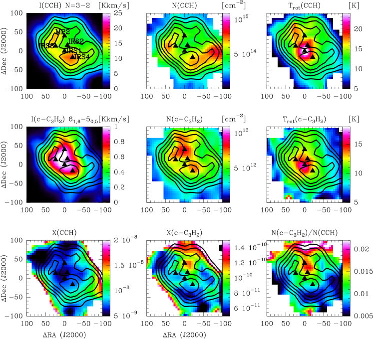
Figure 6: First two rows: Maps of the integrated intensity of the CCH   (262.004$\,\mathrm{GHz}$) and c-C₃H₂   (217.822$\,\mathrm{GHz}$) lines, and of the column density and rotation temperature derived applying the rotational diagram technique to each pixel. Black contours indicate the CCH 3-2 integrated intensity, and go from 5$\,\mathrm{K}$ $\,\mathrm{km\,s^{-1}}$ to 20$\,\mathrm{K}$ $\,\mathrm{km\,s^{-1}}$ in linear steps of 2.5$\,\mathrm{K}$ $\,\mathrm{km\,s^{-1}}$. The position of the infrared sources IRS1/2/3/4 (Henning et al., 1992) and the MP2 position (Ginard et al., 2012) are shown as black triangles. All the maps have been convolved to a spatial resolution of 29″. Bottom row: CCH and c-C₃H₂ abundance maps, obtained using C¹⁸O as a reference and assuming ¹⁶O/¹⁸O = 500 and a CO abundance of $5\times 10^{-5}$ relative to H nuclei. The $N$(c-C₃H₂)/$N$(CCH) ratio is also shown.

In the previous paragraphs we studied the excitation of single positions for all the species and derived some patterns in both the column density and rotational temperature. Here, we generalize the study to the mapping observations. First, we convolved all the maps to the lowest spatial resolution in the mapping dataset (29″). For each pixel in the map, we constructed a rotational diagram for each molecule and derived an excitation temperature and a column density for both CCH and c-C₃H₂. For simplicity, we used only one slope also for CCH. The results are shown in Fig. 6.

For C¹⁸O, our analysis is limited by the fact that the J = 5-4 line was observed only in the NE-SW strip. We have therefore to assume a given $T_{\mathrm{rot}}$ in each pixel based on this dataset. We have interpolated the mean $T_{\mathrm{rot}}$ obtained along the strip to obtain the rotation temperature of C¹⁸O as a function of the distance from the IF. Then we derived the corresponding column densities (Fig. 6) assuming LTE. Since the C¹⁸O emission is optically thin, this yields an estimate of the H₂ column density and allows to normalize the column densities obtained for CCH and c-C₃H₂ to derive their abundances. The corresponding maps are shown in Fig. 6.

To have a deeper insight into the hydrocarbon chemistry we produced a map of $N$(c-C₃H₂)/$N$(CCH), the ratio of the c-C₃H₂ to CCH column densities. The $N$(c-C₃H₂)/$N$(CCH) ratio shows variation up to a factor of 3 across the whole region, being minimum in the bulk of the molecular cloud, then increasing towards the PDR around the HII region and with the maximum located 40″  towards the North, i.e., at the position of the low-UV PDR identified by Ginard et al. (2012). In fact, the $N$(c-C₃H₂)/$N$(CCH) seems to follow the emission of the hot dust (PAH and larger grains) traced by the 8$\,\mathrm{\mu m}$ emission. We can improve the angular resolution of our $N$(c-C₃H₂)/$N$(CCH) image by using directly the CCH 3-2 and c-C₃H₂ 6-5 images (both with an angular resolution of $\sim$10$"$) to derive the $N$(c-C₃H₂)/$N$(CCH) but assuming the CCH and c-C₃H₂ rotation temperatures shown in Fig. 6 although these rotation temperatures were derived with a lower ($\sim$29$"$) angular resolution. Note that the angular resolution of the IRAC 8 $\mu$m image is 2″. This higher resolution $N$(c-C₃H₂)/$N$(CCH) image confirms the correlation with the 8$\mu$m image (see Fig. 7) corroborating the association of an enhanced $N$(c-C₃H₂)/$N$(CCH) with the external part of the PDR. In Sect. 5.2 we will discuss the chemical implications of this correlation.

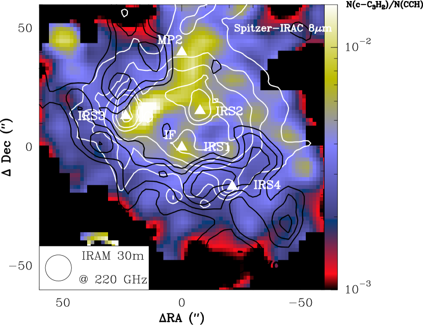
Figure 7: Color image shows the ratio of c-C₃H₂ to CCH column densities as derived from 1mm observations, assuming the rotational temperature of Fig. 6. Pixels without a detection of both CCH and c-C₃H₂ have been masked. The black contours represent the integrated intensity of the 262.004$\,\mathrm{GHz}$ CCH line (from 15 to 25 $\,\mathrm{K\,km\,s^{-1}}$ in steps of 2.5$\,\mathrm{K\,km\,s^{-1}}$), and white contours represent the Spitzer IRAC 8 $\,\mathrm{\mu m}$ emission.

5 Discussion

5.1 Comparison with other PDRs

In the previous section, we have derived the abundances of small hydrocarbons in the different environments of Mon R2. In the PDR, the abundances are $X(\mbox{CH})=3.3\times 10^{-9}$, $X(\mbox{CCH})=1.7\times 10^{-8}$ and $X(\mbox{c-C${}_{3}$H${}_{2}$})=1.4\times 10^{-10}$.

Table 4 shows the comparison of the CCH and c-C₃H₂ abundances in different PDRs. With the exception of the Orion Bar, the CCH abundance is relatively constant in PDRs, in the range $(0.6-1.4)\times 10^{-8}$. The abundance in the PDR of Mon R2 is consistent with these results. However, the envelope better matches with the values found in the Orion Bar (Fuente et al., 1996; Ungerechts et al., 1997; Fuente et al., 2003). The case of the Orion Bar is interesting because, similarly to Mon R2, it is a high-UV PDR with an associated envelope, the background molecular cloud not directly affected by the UV photons from the Trapezium cluster. The abundances for the Orion Bar shown in Table 4 were estimated using low angular resolution observations (29″). The beam of these observations comprises both the high-UV irradiated PDR and the warm envelope which hinders from a reliable comparison with the values in other PDRs. Note, however, that the CCH abundance in the Orion Bar is similar to the mean CCH abundance in Mon R2 (Table 6).

On the other side, the c-C₃H₂ abundance shows a larger variation amongst the various PDRs. Whereas the PDRs with a relatively low $G_{\rm 0}$ show an abundance of $(0.6-1.1)\times 10^{-9}$, NGC 7023 NW and Mon R2 show much lower values, $(0.4-2)\times 10^{-10}$. This is also seen as the trend in the $N$(c-C₃H₂)/$N$(CCH) ratio in the different PDRs. Again, the values in the Orion Bar are more similar to the mean value in Mon R2. The $N$(c-C₃H₂)/$N$(CCH) ratio obtained in the PDRs of Mon R2 is an order of magnitude lower compared to that found in ”classical” PDRs (see, for instance, Pety, 2005) and in the diffuse medium (Gerin et al., 2011), and more similar to the value found in the dense gas surrounding the UCH ii region IRAS 20343+4129 (Fontani et al., 2012).

Table 4: Comparison of CCH and c-C₃H₂ abundances in different PDRs.

	$G_{\rm 0}$	$n_{\mathrm{H_{2}}}$ [$\,\mathrm{cm^{-3}}$ ]	$X$(CCH)	$X$(c-C3H2)	$N$(c-C3H2)/$N$(CCH)	References
MonR2
MonR2 IF			$5.7\times 10^{-9}$	$3.5\times 10^{-11}$	0.006	a,b
MonR2 MP2			$2.6\times 10^{-9}$	$7.6\times 10^{-11}$	0.029	a,b
MonR2 PDR	$5\times 10^{5}$	$3\times 10^{6}$	$1.7\times 10^{-8}$	$1.4\times 10^{-10}$	0.008	a
MonR2 env	1-100	$5\times 10^{4}$	$3.5\times 10^{-9}$	$1.4\times 10^{-11}$	0.004	a
MonR2 red wing			$1.8\times 10^{-8}$	$7.8\times 10^{-10}$	0.04	a
Other PDRs
Horsehead	100	$1\times 10^{5}$	$1.4\times 10^{-8}$	$1.1\times 10^{-9}$	0.08	c
Oph-W	400	$2\times 10^{4}$	$6.0\times 10^{-9}$	$6.0\times 10^{-10}$	0.1	d
IC63	1500	$1\times 10^{5}$	$1.1\times 10^{-8}$	$9.0\times 10^{-10}$	0.08	d
NGC7023	2600	$10^{4}-10^{6}$	$6.0\times 10^{-9}$	$2.0\times 10^{-10}$	0.03	e,f,g
Orion Bar	$2\times 10^{4}$	$1\times 10^{5}$	$2.0\times 10^{-9}$	$3.8\times 10^{-11}$	0.01-0.03	f,h,i

(a): this work; (b): Ginard et al. (2012); (c): Pety et al. (2005) (d) Teyssier et al. (2004); (e) Fuente et al. (1993); (f): Fuente et al. (2003); (g) Pilleri et al. (2012b); (h): Ungerechts et al. (1997); (i): Fuente et al. (1996)

5.2 Comparison with chemical models

In this section, we compare the observational results with the results of different chemical models, in order to qualitatively distinguish which effects may be dominant in the different phases that co-exist in this region. To fully model the chemistry of this complex is beyond the scope of this paper. Our goal is to explore the possible impact of different factors such as the grain-surface chemistry or time dependency, on the carbon chemistry in these environments.

The PDR layers (hereafter, $L_{PDR}$ and $L_{HD}$ for the exposed PDR and the high density PDR, see Fig. 2) have different characteristics, in terms of physical conditions and time scales compared to the cold envelope. We assumed the density structure described in Sect. 2 (see also the top panel in Fig. 8), in which the mainly atomic layer $L_{PDR}$ ($A_{V}<1$, $n_{\mathrm{H_{2}}}=2\times 10^{5}$$\,\mathrm{cm^{-3}}$, $G_{\rm 0}=5\times 10^{5}$) is followed by the high density layer $L_{HD}$ ($1<A_{V}<10$ , $n_{\mathrm{H_{2}}}=3\times 10^{6}$$\,\mathrm{cm^{-3}}$), where many molecular species start to be abundant. These innermost layers are surrounded by the low-density envelope $L_{env}$ ($10<A_{V}<50$, $n_{\mathrm{H_{2}}}=5\times 10^{4}$$\,\mathrm{cm^{-3}}$). The assumption of constant density has to be taken with caution: local variations of gas density (clumps) and smoother gradients are expected to be found in the PDR layers, and the density in the envelope most likely decreases with the distance from the IF. However, this zero-order approximation allows to reduce the free parameters of the modeling to a few, which ease the comparison of models and observational data.

To model the $L_{PDR}$ and $L_{HD}$ layers, we used the Meudon PDR code (Le Petit et al., 2006; Goicoechea & Le Bourlot, 2007; Gonzalez Garcia et al., 2008; Le Bourlot et al., 2012) version 1.4.3 using the density profile shown in Fig. 8. The Meudon Code computes the steady-state solution to the thermal balance and gas-phase chemical networks using accurate radiative transfer calculations and a plane-parallel geometry. The transition between $L_{HD}$ and $L_{PDR}$ is calculated self-consistently by the code. This yields stationary solution for the gas and dust temperature, as well as the abundance of each molecule in each of the layers by assuming equilibrium conditions. Time-dependent effects and gas-grain interactions are not included in the model and therefore its use is justified for the region where chemical equilibrium has already been reached and where gas-grain interaction is not expected to play a major role. However, the Meudon PDR code has very extensive gas-phase chemical networks and is best-suited for studying the gas-phase chemistry of Mon R2.

To study the low-density, cold envelope we used the UCL_CHEM code (Viti et al., 2004). This code includes gas-grain interaction: for the purpose of this paper it is used as a two-phase model which consists of the collapse of a prestellar core (Phase I), followed by the subsequent warming and evaporation of grain mantles due to the enhanced (with respect to the ISRF) radiation field (Phase II). In phase I, a diffuse cloud of density 10² cm^-3 undergoes free-fall collapse until it has reached a final density (set by the user). This phase occurs at a temperature of 10 K. During the collapse, atoms and molecules collide with, and freeze onto, grain surfaces. The advantage of this approach is that the ice composition is not assumed, but it is derived by a time-dependent computation of the chemical evolution of the gas-dust interaction process which, in turns, depends on the density of the gas. Hydrogenation occurs rapidly on grain surfaces, so that, for example, some percentage of carbon atoms accreting will rapidly become frozen out as methane, CH₄.

For all the models we use the same initial elemental abundances (see Table 5). The codes employ the reaction rate data from the UMIST astrochemical database, augmented with grain-surface (hydrogenation) reactions as in Viti et al. (2004) and Viti et al. (2011) for the UCL_CHEM models. In both Phases of this code, non-thermal desorption is also considered as in Roberts et al. (2007).

Table 5: Input parameters for the Meudon PDR code

Parameter		Value
$G_{0}$	Radiation field intensity	$5\times 10^{5}$
$G_{0}^{ext}$	External Radiation field intensity	100
$A_{\rm V}$	Total cloud depth	50 mag
Extinction		Standard Galactic
$R_{V}$	$A_{\rm V}$/$E_{\rm B-V}$	3.1
$\zeta$	Cosmic ray ionization rate	$5\times 10^{-17}$ s-1
$a_{min}$	dust minimum radius	$3\times 10^{-7}$ cm
$a_{max}$	dust maximum radius	$3\times 10^{-5}$ cm
$\alpha$	MRN dust size distribution index	3.5
He/H	Helium abundance	0.1
O/H	Oxygen abundance	$3.2\times 10^{-4}$
C/H	Carbon abundance	$1.3\times 10^{-4}$
N/H	Nitrogen abundance	$7.5\times 10^{-5}$
S/H	Sulfur abundance	$1.8\times 10^{-5}$

5.2.1 Abundances in the PDRs

The column densities and abundances in the PDR obtained from the observations refer to the innermost 10 mag of the PDR. Therefore, we have to compare them with the mean values in the $L_{PDR}$ $+$$L_{HD}$ layer. Another way to study the chemical difference between these species and minimize the uncertainties due to the assumed physical structure is to consider the column density ratios $N(\mbox{CH})/N(\mbox{CCH})$ and $N$(c-C₃H₂)/$N$(CCH) instead of absolute abundances.

In the exposed PDR layer ($L_{PDR}$), the gas temperature and UV field are so high that gas-phase chemistry is expected to be dominant. We can safely assume that all hydrocarbons have evaporated from grain surfaces and that there are no ices, since the dust temperature (100-150$\,\mathrm{K}$, Pilleri et al., 2012a) is above the sublimation limit for all the molecules involved in reactions with hydrocarbons, especially methane (Tielens, 2005).

The results of the Meudon code modeling are displayed in Fig. 8. The model shows that all the hydrocarbons are expected to have their abundance peak at $A_{V}\sim 1$. For CCH, the model predicts a peak abundance of $\sim 10^{-6}$ which rapidly decreases to $10^{-15}$. Similarly, c-C₃H₂ has an abundance peak toward the PDR of $\sim 10^{-10}$ and a decrease to $10^{-15}$. The abundance gradient is less abrupt for CH which passes from a peak of $10^{-8}$ in the PDR to $10^{-12}$ in the more shielded layers of the molecular cloud.

The column densities (and abundances) of CH and CCH are relatively well reproduced by the Meudon PDR code, considering the integrated column density in the two layers $L_{PDR}$ and $L_{HD}$ (see Table 6). Concerning c-C₃H₂, the model predicts a $N$(c-C₃H₂)/$N$(CCH) ratio of 0.0003 while the observed value is of the order of 0.01 in the PDR, which shows that the c-C₃H₂ is overabundant compared to the model predictions. This is consistent with several previous studies showing that in PDRs the gas-phase model predictions cannot account for the observed abundances of small hydrocarbons (Fuente et al., 1993; Teyssier et al., 2004; Pety et al., 2005), especially c-C₃H₂.

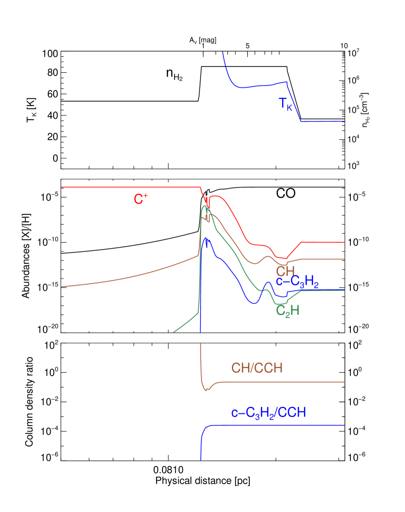
Figure 8: Model results using the gas-phase steady-state chemistry with the Meudon PDR code. The cloud is illuminated from the left side with a UV field of $G_{\rm 0}=5\times 10^{5}$.

A link with PAHs?

A possible way to reduce the discrepancy could be the injection of fresh hydrocarbons by the photo-destruction of PAHs or larger grains (Fuente et al., 2003; Pety, 2005). Indeed, laboratory experiments show that the photodissociation of small PAHs ($N_{\rm C}\leq 24$) can lead to the production of small hydrocarbons C_nH_m ($n>m$) that can be injected into the gas phase (Useli Bacchitta & Joblin, 2007). To understand if PAHs can be linked to a chemical differentiation of CCH and c-C₃H₂, it is useful to compare the ratio between the column density of c-C₃H₂ and CCH with the spatial distribution of PAHs. In Fig. 7 we display the comparison of the $N$(c-C₃H₂)/$N$(CCH) ratio with the IRAC 8$\,\mathrm{\mu m}$ map.

In low- to mild-UV irradiated PDR, the 8$\,\mathrm{\mu m}$ map is dominated by the emission of the AIB at 7.7$\,\mathrm{\mu m}$, but in high-UV excited environments larger grains at thermal equilibrium can reach temperatures high enough to have continuum emission at these wavelength. To check whether this is the case in Mon R2, we have compared the IRAC 8$\,\mathrm{\mu m}$ map with that obtained with the IRAC 3.5$\,\mathrm{\mu m}$ filter, which is expected to be dominated either by the PAH 3.3$\,\mathrm{\mu m}$ feature or by the stellar continuum. The two IRAC maps are very similar, except for very point-like features in correspondence with the infrared source IRS 2 and IRS 3. Therefore, we can assume that most of the IRAC 8$\,\mathrm{\mu m}$ emission is indeed due to AIB emission. Finally, visual inspection of the IRS spectra in the central region of Mon R2 shows that the PAH features dominate the emission at 8$\,\mathrm{\mu m}$, except towards the bright infrared sources. The comparison of the ratio of the c-C₃H₂ and CCH column densities with the spatial distribution of CCH suggests that $i)$ c-C₃H₂ is overabundant in the innermost layers of the cloud, and $ii)$ the c-C₃H₂ spatial distribution extends to the NW, following the northern IR ridge that is observed at 8$\,\mathrm{\mu m}$ (Ginard et al., 2012).

The correlation between the PAH emission and the c-C₃H₂ overabundance, although suggestive of a chemical link between these species, does not prove yet that these two tracers are chemically linked (i.e. by UV processing), since they are both good PDR tracers. For instance, it has been observed that PAH and [C ii ] emission are spatially correlated in PDRs (Joblin et al., 2010), since both tracers arise in the most exposed layers of the PDR. This could also mean that the chemical differentiation of CCH and c-C₃H₂ in PDRs can also be due to an increased abundance of C⁺ in these environments. Furthermore, C ii and PAHs also trace the electron density, which is mainly due to the ionization of C and photo-electric effect on PAHs. Since c-C₃H₂ is supposed to form by electron recombination of the C₃H${}_{3}^{+}$, a higher production efficiency of photo-electrons ejected from PAHs may be a cause of c-C₃H₂ enhancement. However, the inclusion of these effects in PDR models is still very challenging and beyond the scope of this paper.

5.2.2 Low density envelope

Our observations indicate that the abundances of small hydrocarbons in the envelope are about 5-10 times lower compared to the PDR. The column densities of CH and c-C₃H₂ relative to CCH are also a factor of 3 and 2 lower compared to the PDR. Even though, the CCH and c-C₃H₂ abundances are larger by several orders of magnitude than those predicted by steady-stage gas chemical models. In our sketch of MonR2, we assume the envelope to be 40 mag thick on each side of the spherical cloud, with a gas density of $n_{\mathrm{H_{2}}}=5\times 10^{4}$$\,\mathrm{cm^{-3}}$ and a gas kinetic temperature of 35$\,\mathrm{K}$. With these physical conditions, gas-grain chemistry and time-dependent effects may play a role.

To study these processes we used the UCL_CHEM models running Phase 1 from diffuse core up to a density of $n_{\mathrm{H_{2}}}=5\times 10^{4}$$\,\mathrm{cm^{-3}}$, while the temperature and radiation field were kept at 10$\,\mathrm{K}$ and 1 Habing respectively. Once the final density was reached we increased the radiation field to $G_{\rm 0}=100$ and the kinetic temperature to 35$\,\mathrm{K}$ (Phase 2). The model assumes a number of parameters, such as the freeze-out, photo- and thermal-desorption efficiencies. We use the standard values for the different non thermal desorption efficiencies as in Roberts et al. (2007). In particular, the models are strongly dependent on the freeze-out efficiency during phase 1, which determines the initial abundances of CH, CCH and c-C₃H₂  in Phase 2. We have tested the impact of the kinetic temperature in the envelope in the final hydrocarbon abundances, and found no significant difference in the range [10-35]$\,\mathrm{K}$. This is consistent with the fact that at $T_{\rm dust}$=35$\,\mathrm{K}$, most of the species remain in the grain mantles (Viti et al., 2004) and the rates of main gas phase reactions involved in the formation and destruction of hydrocarbons do not present strong variations in this temperature range.

In Fig. 9 we report an example of the time evolution during Phase 2 for an $A_{V}=41$, assuming a low (10%) CO freeze-out. The model predicts that all the hydrocarbon abundances are constant up to $10^{4}$ years. At this time, each of the absolute abundances for CH and CCH are reproduced within a factor of 3 but their ratio is over-predicted by a factor of 7 (see Table 6). Considering the high uncertainties in the absolute column density of CH (driven by the unknown excitation temperature) it is difficult to further constrain the model based on this ratio. After $1\times 10^{4}$ years, gas phase CH decreases by a factor of a few, whereas CCH and c-C₃H₂ decrease by the more than one order of magnitude: for $t\gtrsim 10^{5}$ years, the agreement of $N$(c-C₃H₂)/$N$(CCH)  with observations improves, but the absolute abundances and the CH/CCH ratio do not agree as well as at $1\times 10^{4}$ years.

Repeating the calculations for higher freeze-out fractions (25% and 45%, see Table 6) one can find a better agreement for one or the other molecule, but it is difficult to find a solution that fits reasonably well all the abundances or column densities.

In any case, the chemistry of Mon R2 seems to be dominated by grain-surface processes and time-dependent effects, since at the age of UCHII region ($\sim$0.1 Myr) the molecular chemistry is far from the steady state yet. In this scenario the current abundances of small hydrocarbons are dependent on the previous history of the cloud. This is consistent with recent results of Mookerjea et al. (2012), who studied these effects in the envelope associated with DR21. They investigated the impact of time-dependent effects for the carbon chemistry of this warm cloud, showing that PAH-related chemistry is not needed to explain the abundances of neither CCH or c-C₃H₂ in this molecular envelope.

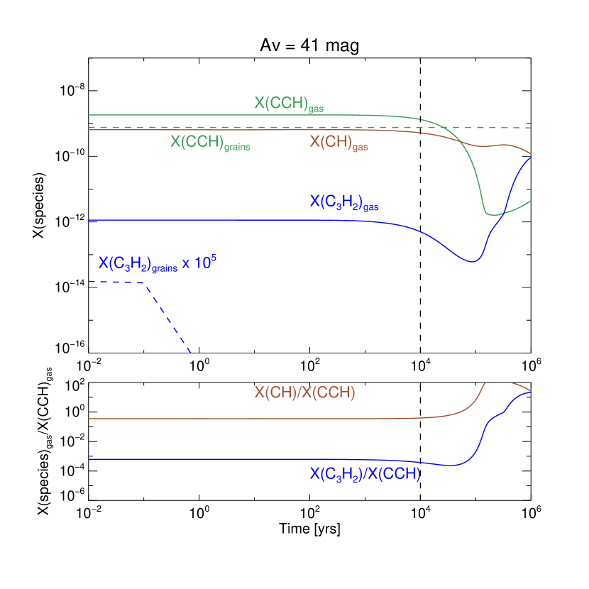
Figure 9: Results of the UCL CHEM code to model the low-density envelope $L_{HD}$  for a starting CO freeze-out of 10%. The results are given at $A_{V}$ of 41 magnitudes and by setting the temperature fixed to 35$\,\mathrm{K}$. The bottom panel shows the ratio of gas-phase CH and c-C₃H₂ relative to CCH. The vertical dashed line marks the age of $10^{4}$ years, which is used in Table 6

.

Table 6: Comparison between the abundances derived from observations and model predictions. For the UCL_CHEM code, we show the results at $t=10^{4}$ years.

	$A_{V}$	$X$(CH)	$X$(CCH)	$X$(c-C3H2)	$N(\mbox{CH})/N(\mbox{CCH})$	$N$(c-C3H2)/$N$(CCH)
	[mag]
$X_{obs}^{PDR}$	1-10	$3.3^{+6.0}_{-2.2}\times 10^{-9}$	$1.7\times 10^{-8}$	$1.4\times 10^{-10}$	0.15	0.008
Meudon $L_{PDR}$ +$L_{HD}$	1-10	$1.1\times 10^{-8}$	$4.8\times 10^{-8}$	$1.3\times 10^{-11}$	0.22	0.00025
$X_{obs}^{env}$	10-50	$1.9^{+3.3}_{-1.2}\times 10^{-10}$	$3.5\times 10^{-9}$	$1.4\times 10^{-11}$	0.054	0.004
UCL_CHEM $L_{env}$ f = 10	41	$5.1\times 10^{-10}$	$1.3\times 10^{-9}$	$4.8\times 10^{-13}$	0.39	0.0004
UCL_CHEM $L_{env}$ f = 25	41	$9.5\times 10^{-10}$	$6.9\times 10^{-10}$	$3.5\times 10^{-11}$	1.37	0.05
UCL_CHEM $L_{env}$ f = 45	41	$7.5\times 10^{-10}$	$3.5\times 10^{-10}$	$1.4\times 10^{-10}$	2.1	0.40

6 Conclusions

In this paper, we have presented new observations of small hydrocarbon molecules (CH, CCH and c-C₃H₂) in MonR2 obtained with the IRAM-30m telescope and the HIFI instrument onboard Herschel. In particular, the HIFI observations allowed to access the N=6-5 rotational transitions of CCH with a good spatial and spectral resolution. This allowed to constrain the excitation conditions and to distinguish the different phases in which this species is abundant. Profiting of a multi-transition and spatial study, we have derived the spatial distribution of these molecules, determining their abundances in the different layers of Mon R2.

We compared the observational results with predictions of different PDR models, to investigate which kind of chemistry can dominate in the different environments that co-exist in MonR2:

• In the high-UV illuminated PDR, grain mantles have already been evaporated and we can safely assume that chemical equilibrium has been reached. In this case, the gas-phase chemistry can explain quite well the abundances of CH and CCH but fails to reproduce c-C₃H₂. The chemical differentiation of these two molecules happens in correspondence with PAH emission, suggesting once again a link between these species.

• In the cold ($\sim 35\,\mathrm{K}$) low-density molecular cloud, time dependent effects seems to be very important: around $10^{4}$ years, the abundances predicted by the models are relatively consistent with those derived from the observations. At this time all the absolute abundances are relatively well reproduced, although CH is over-predicted relative to both CCH and c-C₃H₂. These models are however strongly dependent on the initial abundances due to the freeze-out in the cloud collapse phase.

This study shows that several effects must be taken into account to understand the chemistry of small hydrocarbons such as CCH and c-C₃H₂: the relative contribution of UV radiation, grain-surface chemistry and time-dependent effects may vary in different environments. Regarding PDRs, a more detailed analysis of the small hydrocarbon chemistry in these environments requires: $(i)$ a larger sample of PDRs spanning a large range of physical conditions to minimize effects due to a peculiar geometry of a particular source; $(ii)$ to revise the possible chemical routes to the formation of small hydrocarbons such as the photo-destruction of PAHs, and very small grains. Herschel data will allow to constrain the hydrocarbons chemical models, including related species that are not observable from the ground (e.g., C⁺, CH⁺). Finally ($iii$) higher resolution observations with the Plateau de Bure Interferometer, NOEMA, ALMA and JCMT will allow to observe several key species with an unprecedented spatial resolution. This will enable to resolve the small-scale chemical frontiers in the PDR that seems to be key interpret the link between small hydrocarbons and PAHs.

Appendix A Diffuse gas in the line of sight

The low-lying transitions of all the hydrocarbons show a clear self-absorption at about the velocity of $\sim$11$\,\mathrm{km\,s^{-1}}$ toward the IF (see Fig. 3). A similar, narrow self-absorption component has also been reported for the [C ii ] 158$\,\mathrm{\mu m}$ line (Pilleri et al. 2012a; Ossenkopf et al. 2013). This feature suggests the presence of a relative diffuse phase in the line of sight. The velocity at which the absorption features appears is the same as that of the emission of the quiescent molecular cloud. Thus, it is likely that this absorbing layer is a low-density gas associated with the most external layer of the molecular cloud.

To determine the column density of the absorbing gas, we need to estimate a reference for the spectral profile of the emission line. We assume that the widths of the lines belonging to a species are similar, and use a transition that is less affected by self-absorption to estimate the FWHM of a gaussian profile. We obtain a FWHM of 5.5$\,\mathrm{km\,s^{-1}}$ for CCH (using the J = 87.407$\,\mathrm{GHz}$ line) and 3$\,\mathrm{km\,s^{-1}}$ for c-C₃H₂ (using the 150.820$\,\mathrm{GHz}$ line) and 6$\,\mathrm{km\,s^{-1}}$ for CH. Using these line widths, we can adjust the blue-shifted wing of the self-absorbed line with a gaussian and use it as reference to calculate the integrated opacity of the self-absorption. By assuming an excitation temperature $T_{ex}=2.73\,\mathrm{K}$, we derive column densities associated to the foreground of $N(\mbox{CH})=4.8\times 10^{13}$$\,\mathrm{cm^{-2}}$ $N(\mbox{CCH})=5.0\times 10^{13}$$\,\mathrm{cm^{-2}}$ and $N(\mbox{c-C${}_{3}$H${}_{2}$})=1.4\times 10^{12}\,\mathrm{cm^{-2}}.$

From CH, we can derive the H₂ column density associated with the absorption, hence an estimate of the extinction. The standard abundance of CH relative to H₂ in diffuse gas is $3.5\times 10^{-8}$ (Sheffer et al. 2008), which leads to a molecular hydrogen column density of $N(\mbox{H${}_{2}$})\sim 1.3\times 10^{21}$$\,\mathrm{cm^{-2}}$ or about 1.3 mag of extinction. This yields CCH and c-C₃H₂ abundances (relative to H₂) of $3.9\times 10^{-8}$ and $1.6\times 10^{-9}$, respectively. These values are consistent with the typical values observed in diffuse gas (Liszt & Lucas 2002; Gerin et al. 2011). The results are similar when considering an offset of [20″,20″], where the self-absorption is still detected with a sufficient S/N to infer relatively accurate column densities.

These estimates suffer from the uncertainty due to the assumed line profile and on the observed continuum. Nevertheless, the detection of this foreground, 1$A_{V}$ thick layer associated with the external layer of the envelope is interesting and moves toward a deeper understanding of this source.

Appendix B Spectroscopic parameters, maps and rotational diagrams

Table 7: Spectroscopic parameters of the observed transitions

Transition	Frequency	Eu	Aul	$g_{u}$
	[$\,\mathrm{GHz}$ ]	$[$K$]$	[s-1]
CH $2\Pi_{1/2}$, $N=1$, $J=3/2-1/2$
P = $2^{-}-1^{+}$	536.76115	0.00072	0.0638	5
P = $1^{-}-1^{+}$	536.78195	0.00072	0.0213	3
P = $1^{-}-0^{+}$	536.79568	0.0	0.0425	3
CH $2\Pi_{1/2}$, $N=2$, $J=5/2-3/2$
P = $3^{+}-2^{-}$	1656.961	25.727	0.03719	7
P = $2^{+}-2^{-}$	1656.970	25.727	0.00372	5
P = $2^{+}-1^{-}$	1656.972	25.727	0.03348	5
CCH $N=1-0$
J=3/2-1/2, F= 1-1	87.28410	0.00216	$2.5920\times 10^{-7}$	3
J=3/2-1/2, F= 2-1	87.31690	0.00216	$1.5274\times 10^{-6}$	5
J=3/2-1/2, F= 1-0	87.32859	0.00000	$1.2684\times 10^{-6}$	3
J=1/2-1/2, F= 1-1	87.40199	0.00216	$1.2715\times 10^{-6}$	3
J=1/2-1/2, F= 0-1	87.40716	0.00216	$1.5324\times 10^{-6}$	1
CCH $N=3-2$
J=7/2-5/2, F=4-3	262.00426	12.57513	$5.30542\times 10^{-5}$	9
J=7/2-5/2, F=3-2	262.00648	12.57383	$5.10470\times 10^{-5}$	7
J=5/2-3/2, F=3-2	262.06499	12.58203	$4.87506\times 10^{-5}$	7
J=5/2-3/2, F=2-1	262.06747	12.58261	$4.45975\times 10^{-5}$	5
CCH $N=6-5$
J=13/2-11/2, F=7-6	523.97157	62.87103	$4.5697\times 10^{-4}$	15
J=13/2-11/2, F=6-5	523.97217	62.86987	$4.5179\times 10^{-4}$	13
J=11/2-9/2, F=6-5	524.03390	62.88685	$4.4939\times 10^{-4}$	13
J=11/2-9/2, F=5-4	524.03453	62.88757	$4.4205\times 10^{-4}$	11
c-C3H2 $J_{K_{A},K_{C}}=2_{1,2}-1_{0,1}$	85.33889	4.1	$2.55335\times 10^{-5}$	15
c-C3H2 $J_{K_{A},K_{C}}=4_{0,4}-3_{1,3}$	150.82067	19.3	$1.79933\times 10^{-4}$	9
c-C3H2 $J_{K_{A},K_{C}}=4_{1,4}-3_{0,3}$	150.85191	17.0	$1.80086\times 10^{-4}$	27
c-C3H2 $J=6-5$
${K_{A},K_{C}}=1,6-0,5$	217.82215	36.3	$5.93376\times 10^{-4}$	39
${K_{A},K_{C}}=0,6-1,5$	217.82215	38.6	$5.93403\times 10^{-4}$	13
c-C3H2 $J_{K_{A},K_{C}}=5_{1,4}-4_{2,3}$	217.94005	33.1	$4.42680\times 10^{-4}$	33
c-C3H2 $J_{K_{A},K_{C}}=4_{3,2}-3_{2,1}$	227.16913	26.7	$3.42484\times 10^{-4}$	27
c-C3H2 $J=7-6$
${K_{A},K_{C}}=0,7-1,6$	251.31434	48.3	$9.34953\times 10^{-4}$	45
${K_{A},K_{C}}=1,7-0,6$	251.31434	50.7	$9.34781\times 10^{-4}$	15
c-C3H2 $J=6-5$
${K_{A},K_{C}}=2,5-1,4$	251.52730	45.1	$7.42318\times 10^{-4}$	39

References: CH: (McCarthy et al. 2006) & CDMS; CCH: (Padovani et al. 2009) & CDMS; c-C₃H₂: JPL

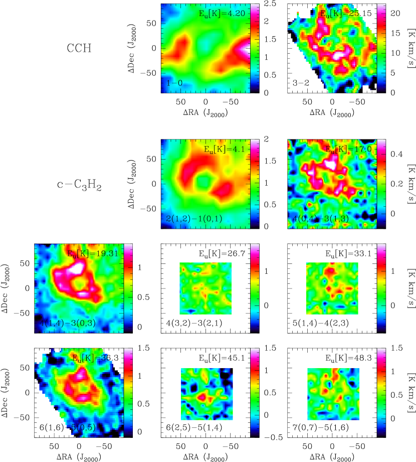
Figure 10: Integrated intensity of all the observed c-C₃H₂ and CCH transitions. The upper state energy level and the principal quantum numbers are shown for each transition. The smaller-scale maps have been convolved to the spatial resolution of 15″to improve the S/N ratio.

.

References

- Berné et al. (2009) Berné, O., Fuente, A., Goicoechea, J. R., et al. 2009, ApJ, 706, L160
- Cernicharo (2012) Cernicharo, J. 2012, in Proceedings of the European Conference on Laboratory Astrophysics, Eur. Astron. Soc. Publ. Ser, ed. C. Stehlé, C. Joblin, & L. d’Hendecourt
- Chandra & Kegel (2000) Chandra, S. & Kegel, W. H. 2000, A&AS, 142, 113
- Choi et al. (2000) Choi, M., Evans, II, N. J., Tafalla, M., & Bachiller, R. 2000, ApJ, 538, 738
- de Graauw et al. (2010) de Graauw, T., Helmich, F. P., Phillips, T. G., et al. 2010, A&A, 518, L6
- Fontani et al. (2012) Fontani, F., Palau, A., Busquet, G., et al. 2012, MNRAS, 423, 1691
- Fuente et al. (2010) Fuente, A., Berné, O., Cernicharo, J., et al. 2010, A&A, 521, L23
- Fuente et al. (1993) Fuente, A., Martin-Pintado, J., Cernicharo, J., & Bachiller, R. 1993, A&A, 276, 473
- Fuente et al. (2003) Fuente, A., Rodrıguez-Franco, A., Garcıa-Burillo, S., Martın-Pintado, J., & Black, J. H. 2003, A&A, 406, 899
- Fuente et al. (1996) Fuente, A., Rodriguez-Franco, A., & Martin-Pintado, J. 1996, A&A, 312, 599
- Gerin et al. (2011) Gerin, M., Kaźmierczak, M., Jastrzebska, M., et al. 2011, A&A, 525, A116
- Ginard et al. (2012) Ginard, D., González-García, M., Fuente, A., et al. 2012, A&A, 543, A27
- Goicoechea & Le Bourlot (2007) Goicoechea, J. R. & Le Bourlot, J. 2007, A&A, 467, 1
- Gonzalez Garcia et al. (2008) Gonzalez Garcia, M., Le Bourlot, J., Le Petit, F., & Roueff, E. 2008, A&A, 485, 127
- Habing (1968) Habing, H. J. 1968, Bull. Astron. Inst. Netherlands, 19, 421
- Henning et al. (1992) Henning, T., Chini, R., & Pfau, W. 1992, A&A, 263, 285
- Joblin et al. (2010) Joblin, C., Pilleri, P., Montillaud, J., et al. 2010, A&A, 521, L25
- Le Bourlot et al. (2012) Le Bourlot, J., Le Petit, F., Pinto, C., Roueff, E., & Roy, F. 2012, A&A, 541, A76
- Le Petit et al. (2006) Le Petit, F., Nehmé, C., Le Bourlot, J., & Roueff, E. 2006, ApJS, 164, 506
- Liszt & Lucas (2002) Liszt, H. & Lucas, R. 2002, A&A, 391, 693
- Loren (1977) Loren, R. B. 1977, ApJ, 215, 129
- Lucas & Liszt (2000) Lucas, R. & Liszt, H. S. 2000, A&A, 358, 1069
- McCarthy et al. (2006) McCarthy, M. C., Mohamed, S., Brown, J. M., & Thaddeus, P. 2006, Proceedings of the National Academy of Science, 103, 12263
- Mookerjea et al. (2012) Mookerjea, B., Hassel, G. E., Gerin, M., et al. 2012, A&A, 546, A75
- Ossenkopf et al. (2011) Ossenkopf, V., Röllig, M., Kramer, C., et al. 2011, in EAS Publications Series, Vol. 52, EAS Publications Series, ed. M. Röllig, R. Simon, V. Ossenkopf, & J. Stutzki, 181–186
- Ossenkopf et al. (2013) Ossenkopf, V., Röllig, M., Neufeld, D. A., et al. 2013, A&A, 550, A57
- Ott (2010) Ott, S. 2010, in Astronomical Society of the Pacific Conference Series, Vol. 434, Astronomical Data Analysis Software and Systems XIX, ed. Y. Mizumoto, K.-I. Morita, & M. Ohishi, 139
- Padovani et al. (2009) Padovani, M., Walmsley, C. M., Tafalla, M., Galli, D., & Müller, H. S. P. 2009, A&A, 505, 1199
- Penzias & Burrus (1973) Penzias, A. A. & Burrus, C. A. 1973, ARA&A, 11, 51
- Pety (2005) Pety, J. 2005, in SF2A-2005: Semaine de l’Astrophysique Francaise, ed. F. Casoli, T. Contini, J. M. Hameury, & L. Pagani, 721
- Pety et al. (2005) Pety, J., Teyssier, D., Fossé, D., et al. 2005, A&A, 435, 885
- Pilbratt et al. (2010) Pilbratt, G. L., Riedinger, J. R., Passvogel, T., et al. 2010, A&A, 518, L1
- Pilleri et al. (2012a) Pilleri, P., Fuente, A., Cernicharo, J., et al. 2012a, A&A, 544, A110
- Pilleri et al. (2012b) Pilleri, P., Montillaud, J., Berné, O., & Joblin, C. 2012b, A&A, 542, A69
- Rizzo et al. (2003) Rizzo, J. R., Fuente, A., Rodríguez-Franco, A., & García-Burillo, S. 2003, ApJ, 597, L153
- Roberts et al. (2007) Roberts, J. F., Rawlings, J. M. C., Viti, S., & Williams, D. A. 2007, MNRAS, 382, 733
- Roelfsema et al. (2012) Roelfsema, P. R., Helmich, F. P., Teyssier, D., et al. 2012, A&A, 537, A17
- Sheffer et al. (2008) Sheffer, Y., Rogers, M., Federman, S. R., et al. 2008, ApJ, 687, 1075
- Spielfiedel et al. (2012) Spielfiedel, A., Feautrier, N., Najar, F., et al. 2012, MNRAS, 421, 1891
- Tafalla et al. (1994) Tafalla, M., Bachiller, R., & Wright, M. C. H. 1994, ApJ, 432, L127
- Tafalla et al. (1997) Tafalla, M., Bachiller, R., Wright, M. C. H., & Welch, W. J. 1997, ApJ, 474, 329
- Teyssier et al. (2004) Teyssier, D., Fossé, D., Gerin, M., et al. 2004, A&A, 417, 135
- Tielens (2005) Tielens, A. G. G. M. 2005, The Physics and Chemistry of the Interstellar Medium
- Treviño-Morales, et al. (2012) Treviño-Morales, et al. 2012, A&A, in preparation
- Ungerechts et al. (1997) Ungerechts, H., Bergin, E. A., Goldsmith, P. F., et al. 1997, ApJ, 482, 245
- Useli Bacchitta & Joblin (2007) Useli Bacchitta, F. & Joblin, C. 2007, in Molecules in Space and Laboratory, ed. P. J.L. Lemaire & F. Combes, publ. S. Diana, 89
- Viti et al. (2004) Viti, S., Collings, M. P., Dever, J. W., McCoustra, M. R. S., & Williams, D. A. 2004, MNRAS, 354, 1141
- Viti et al. (2011) Viti, S., Jimenez-Serra, I., Yates, J. A., et al. 2011, ApJ, 740, L3