“RADIOASTRON” — A TELESCOPE WITH A SIZE OF 300 000 KM:
MAIN PARAMETERS AND FIRST OBSERVATIONAL RESULTS

Abstract

The Russian Academy of Sciences and Federal Space Agency, together with the participation of many international organizations, worked toward the launch of the RadioAstron orbiting space observatory with its onboard 10-m reflector radio telescope from the Baikonur cosmodrome on July 18, 2011. Together with some of the largest ground-based radio telescopes and a set of stations for tracking, collecting, and reducing the data obtained, this space radio telescope forms a multi-antenna ground–space radio interferometer with extremely long baselines, making it possible for the first time to study various objects in the Universe with angular resolutions a million times better than is possible with the human eye. The project is targeted at systematic studies of compact radio-emitting sources and their dynamics. Objects to be studied include supermassive black holes, accretion disks, and relativistic jets in active galactic nuclei, stellar-mass black holes, neutron stars and hypothetical quark stars, regions of formation of stars and planetary systems in our and other galaxies, interplanetary and interstellar plasma, and the gravitational field of the Earth. The results of ground-based and inflight tests of the space radio telescope carried out in both autonomous and ground–space interferometric regimes are reported. The derived characteristics are in agreement with the main requirements of the project. The astrophysical science program has begun.

1 INTRODUCTION

A method for obtaining very high angular resolution in radio astronomy and a specific scheme for the realization of this method are presented in [1–3]. It was noted that radio interferometers on Earth and in space could operate with very long baselines between antennas, with independent registration of the signals at each antenna. Such radio interferometers were first operated in 1967 in Canada [4] and the USA [5]. The first trans-continental interferometers were realized in 1968–1969, between telescopes in the USA and Sweden [6], and also between the Deep Space Network antennas in the USA and Australia [7, 8]. Some of the first observations with trans-continental radio interferometers were carried out jointly by radio astronomers in the USSR and USA in 1969, using the 43-m Green Bank radio telescope (USA) and the 22-m Simeiz telescope (USSR) [9, 10]. Such observations were subsequently carried out between all continents. Modern trans-continental radio interferometers can achieve angular resolutions of fractions of a milliarcsecond (mas). These observations show that most active galactic nuclei (AGNs) possess unresolved components, even on the longest projected ground baselines (approximately 10 000 km); see, e.g., [11, 12] and references therein.

The possibility of creating space interferometers was discussed at a scientific session of the Division of General Physics and Astronomy of the USSR Academy of Sciences on December 23, 1970 [13]. The first Earth–Space interferometer projects emerged at that time. In the 1970s, the Space Research Institute of the USSR Academy of Sciences (IKI) working jointly with industrial partners created the first space radio telescope (SRT), which had a 10-m diameter reflector. This telescope had a trussed, opening construction with a reticulated reflecting surface and receivers tuned to 12 and 72 cm. This radio telescope was delivered to the Salyut-6 manned orbital station by the cargo ship Progress in Summer 1979, where it was tested using astronomical objects with the participation of the cosmonauts V.A. Lyakhov and V.V. Ryumin [14, 15]. One of the outcomes of these experiments was the decision to use a rigid reflecting surface for the RadioAstron project.

A decree of the Council of Ministers of the USSR announcing the development of six spacecraft for astrophysical investigations at the Lavochkin Scientific and Production Association was made in 1980. These included the decimeter- and centimeter-wavelength interferometer RadioAstron (the Spektr-R project), as well as the millimeter and submillimeter radio telescope Millimetron (the Spektr-M project) [16]. The technical specifications for the RadioAstron project had already been prepared in 1979. The first international conference on this project took place in Moscow on December 17-18, 1985. Agreements were signed, and an international group concerned with the development of onboard radio-astronomy receivers based on sets of individual technical specifications was formed. These technical specifications were developed and issued in 1984–1985 by the Astrophysics Division of IKI, headed by I.S. Shklovskii. The group included specialists from the USSR, the Netherlands, the Federal Republic of Germany, Australia, Finland, and India. In the early 1990s, the flight models of the first receivers at 1.35, 6.2, and 18 cm and onboard blocks of input low-noise amplifiers (LNAs) for the 92-cm receiver were delivered to the Astro Space Center of the Lebedev Physical Institute (ASC; formed in 1990 from the IKI Astrophysics Division and the Radio Astronomy Station of the Lebedev Physical Insitute in Pushchino). The 18-cm receiver and 92-cm amplifier blocks form part of the complex of scientific equipment used with the RadioAstron SRT in flight today.

The first successful space interferometer was realized in 1986–1988 using the 5-m diameter antenna of the NASA TDRSS geostationary satellite (USA), which operated at 2 and 13 cm, together with several ground-based radio telescopes [17, 18]. The first SRT specially designed for interferometry was the HALCA satellite of the VSOP project, launched by Japan in 1997 [19, 20]. This 8-m diameter antenna was mounted on a satellite that orbited the Earth in an elliptical orbit with a period of 6.3 hr and a maximum distance from the center of the Earth of 28 000 km. This SRT successfully functioned at wavelengths of 6 and 18 cm until 2003. Both of these space interferometers confirmed not only the possibility, but also the scientific necessity of further developing ground–space radio Very Long Baseline Interferometry (VLBI), in particular of enhancing the angular resolution obtained by increasing the size of the orbit and of expanding the range of wavelengths observed. All of this experience was taken into account when preparing the RadioAstron project.

The RadioAstron SRT is a 10-m diameter reflecting antenna equipped with a complex of 1.35, 6.2, 18, and 92 cm receivers. A Navigator module space platform was used to install the RadioAstron antenna and equipment complex into the Spektr-R spacecraft [21–25]. The arrangement of the SRT and equipment complex in the Navigator module is shown in Fig. 1. A general block schematic of the antenna and equipment complex of the SRT is shown in Fig. 2. The precision carbon-fiber panels of the main antenna of the SRT were manufactured and tested in Russia, and then at the European Space Research and Technology Center (ESTEC) of the European Space Agency in 1994 (Nordwijk, the Netherlands; Fig. 4a). Tests of the model SRT and the equipment complex of the interferometer (Fig. 4b) were carried out from Autumn 2003 through Summer 2004 at the Pushchino Radio Astronomy Observatory (PRAO) of the ASC. The main parameters of the model SRT were measured during these tests using observations of astronomical radio sources, and test observations in an interferometric regime were carried out using the SRT together with the PRAO 22-m radio telescope. This 22-m radio telescope was subsequently outfitted with additional equipment enabling its use as a ground station for tracking the Spektr-R spacecraft in flight. The last ground tests of the SRT with the Navigator module occured at the Lavochkin Association (Figs. 4c,d). At the suggestion of the International Grote Reber Foundation, a memorial plate with a portrait of the pioneer radio astronomer Grote Reber (1911–2002) was installed on the SRT (Fig. 4e). A poster with an image of symbols of the organizations and countries participating in the RadioAstron project was placed on the fairing of the Zenit-3F rocket used to launch the Spektr-R spacecraft (Fig. 4f). Figs. 4g–4i show the transport of the rocket carrier with the Spektr-R spacecraft and the Fregat booster to the launch position.

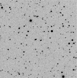
Figure 5: The two elliptical images near the center of the photograph show the Fregat booster (on the right) and the spacecraft which has separated from it (on the left). The photograph was made on July 18, 2011, at 14:25 (Moscow daylight saving time) using a 45.5-cm optical telescope in New Mexico at the request of the Keldysh Institute of Applied Mathematics. This telescope is part of the Scientific Network of Optical Instruments for Astrometric and Photometric Observations, and is designed to search for asteroids and comets.

The launch of the Zenit-3F rocket with the Spektr-R spacecraft took place on July 18, 2011 at 5 hr 31 min 17.91 s Moscow daylight saving time, from the 45th launch pad of the Baikonur cosmodrome (Figs. 4j–4k). On that same day at 14:25, the booster and spacecraft, which had separated from it, were photographed using a 45.5-cm optical telescope in New Mexico, at the request of the Keldysh Institute of Applied Mathematics (IAM) of the Russian Academy of Sciences (Fig. 5). The SRT was successfully deployed on July 23, 2011 (a general view of the Spektr-R spacecraft in space is shown in Fig. 4l). After this, it was possible to begin the inflight tests planned for the first six months of flight: verifying the functioning of the service systems and the scientific equipment of the spacecraft, measuring and updating the characteristics of the orbit, measuring the main parameters of the SRT, searching for fringes in the ground–space interferometer signal, and beginning the Early Science Program (ESP) of astrophysical investigations.

Let us now present a brief history of key astronomical observations in the first half year of the inflight tests of the SRT. The radio-astronomy receivers were successfully turned on for the first time in mid-September 2011, and regular tests of the onboard scientific equipment were begun. Radiometric measurements of the parameters of the SRT using radio-astronomical methods and observations of various astronomical objects during operation of the SRT in a single-dish regime began on September 27, 2011 (Figs. 7a, 7b, 8a–8c). The adjustment and testing of the high-data-rate radio channel for transmitting data between the SRT and the ground tracking station in Pushchino in an interferometric regime were conducted in parallel. Measurements at 92, 18, 6.2, and 1.35 cm began with observations of the Cassiopeia A supernova remnant (Figs. 7a, 8a, 8b), then went on to observations of Jupiter, the Moon, the Crab Nebula (Fig. 7b), the Seyfert galaxy 3C 84, and the quasars 3C 273 and 3C 279, as well as cosmic masers (Figs. 9a–9c) and pulsars (Figs. 7f, 7g, 10). Tests of the ground–space radio interferometer at 18, 6.2, 92, and then 1.35 cm began with observations of the quasar 0212${+}$735 at 18 cm on November 15, 2011 (Fig. 7c). These tests were conducted at various distances of the SRT from the Earth, from the minimum distance to the maximum distance of about 330 000 km, and using observations of various extragalactic and Galactic objects: quasars and galaxies, pulsars, and molecular maser sources radiating in narrow radio lines (Figs. 7c–7f).

Further, we describe the construction of the SRT and the configuration of the onboard science complex (Section 2); the launch and inflight tests of the Spektr-R spacecraft and ground control complex (Section 3); the parameters of the orbit and the means used to measure and refine them (Section 4); measurement of the main parameters of the SRT based on astronomical sources (Section 5); and verification of the functioning of the ground–space interferometer (first fringes) and the first observational results (Section 6). In conclusion, we list directions for further studies. The Appendix presents a possible interpretation of the antenna measurements at 1.35 cm.

2 CONSTRUCTION OF THE SRT AND CONFIGURATION OF THE ONBOARD SCIENCE COMPLEX

The automated Spektr-R spacecraft was designed to carry an SRT to be used as an orbiting element in ground–space VLBI experiments. It includes the Navigator service module (with the Lavochkin Association as the lead organization) [21] and a science complex containing the scientific equipment to be used for the international RadioAstron project (with the ASC as the lead organization) together with the 10-m parabolic antenna itself (jointly developed by the Lavochkin Association and the ASC) [22, 23]. In addition, the spacecraft carried the scientific equipment associated with the Plazma-F project (with IKI as the lead organization), designed for studies of cosmic plasma along the orbit of Spektr-R (this equipment and experiment are described in [26, 27]).

2.1 Construction of the Antenna

The design of the SRT antenna was based on the need to fit the deployable 10-m reflector in its folded state into the payload compartment of the rocket underneath the fairing, which has a specified internal diameter of 3.8 m, and also to ensure the required precision of the reflecting surface after its deployment. According to the technical specifications, the maximum allowed deviation (tolerance) of the dish surface of the radio telescope from the profile for an ideal paraboloid of rotation under all conditions is ${\pm}2$ mm [28]. The reflecting surface is formed of the central part of the dish, with a diameter of 3 m, and 27 radial petal segments, which open synchronously in orbit.

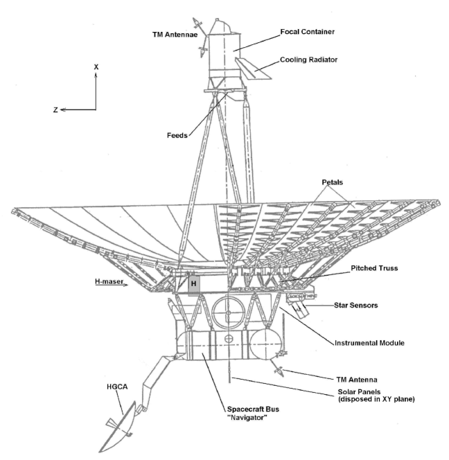
Figure 1: Arrangement of the SRT in the Navigator basic module.

A general schematic of the components of the SRT in the Spektr-R spacecraft is presented in Fig. 1. The main structural elements of the dish are the following:

– focal module truss (serves to regulate the position of the feedhorns);

– reflector truss (fastens the focal module to the focal container);

– cylindrical compartment (designed to fix the central dish and the reflector-petal opening mechanism, and also to house the two onboard hydrogen masers);

– a transitional truss between the SRT and the Navigator service module (used for the installation of the scientific-equipment container).

The petal positions were aligned on the ground before launch, to allow the creation of the precision reflecting surface upon deployment. This was carried out in two stages. In the first, each petal was adjusted individually using adjustment screws at 45 points on a specialized weight-unloading support, taking into account the mass and the position of the axis of rotation of the petal. In the second, the positions of the petals were aligned after assembling the reflector, by varying the lengths of struts fixed to the positions of the petals in the open state. The central dish was fixed on a cylindrical compartment using nine regulating support units. Measurements showed that, after the alignment on the ground, in the presence of backlash and taking into account uncertainties in the manufacture and weight distribution, the maximum deviation of the reflector surface from the theoretical shape of a paraboloid did not exceed ${\pm}1$ mm.

A thermal regulation system (TRS) for the petals, cylindrical compartment, focal and scientific containers, focal unit, and onboard hydrogen masers was designed, to ensure reliable functioning of the instrumentation complex and minimization of thermal structural deformations [29]. A cold plate with the blocks of LNAs for the 1.35, 6.2, and 18-cm receivers mounted on it was connected to the antenna-feed assembly (AFA) and installed in the focal unit of the SRT; the TRS radiator of the cold plate was installed in the shaded side of the focal container (Fig. 1). The TRS of the cold plate was designed to provide the required thermal regime for the LNAs and the central part of the AFA: maintaining the temperatures of the LNA sites between 90 and 150 K, and the sites of the antenna feeds (for 1.35, 6.2, and 18 cm) between 130 and 200 K, throughout the normal operation of the SRT. The geometrical area of shadowing of the SRT dish by the TRS cold-plate radiator does not exceed 1 m². The maximum thermal energy deposited onto the cold plate from the LNAs is no greater than 0.3 W. Heat flow due to thermal connections with other structural elements of the SRT is from 5 to 15 W (this varies primarily with the position of the SRT relative to the Sun). There is a thermal connection between the LNAs and AFA along waveguides and cables. According to housekeeping data, the temperature regimes for the cylindrical compartment, containers, focal unit, and onboard hydrogen masers of the SRT in flight correspond to the projected requirements.

2.2 Onboard Science Complex

The onboard science complex was constructed starting in 1985, as a collaboration between Soviet and foreign organizations. This was carried out in accordance with the general technical requirements for the design of scientific equipment for the Spektr-R spacecraft and the technical specifications for the specific scientific instruments developed by the lead organization for the RadioAstron project — the Astrophysics Division of IKI, which became the Astro Space Center of the Lebedev Physical Institute in 1990. The spacecraft was designed at the Lavochkin Association.

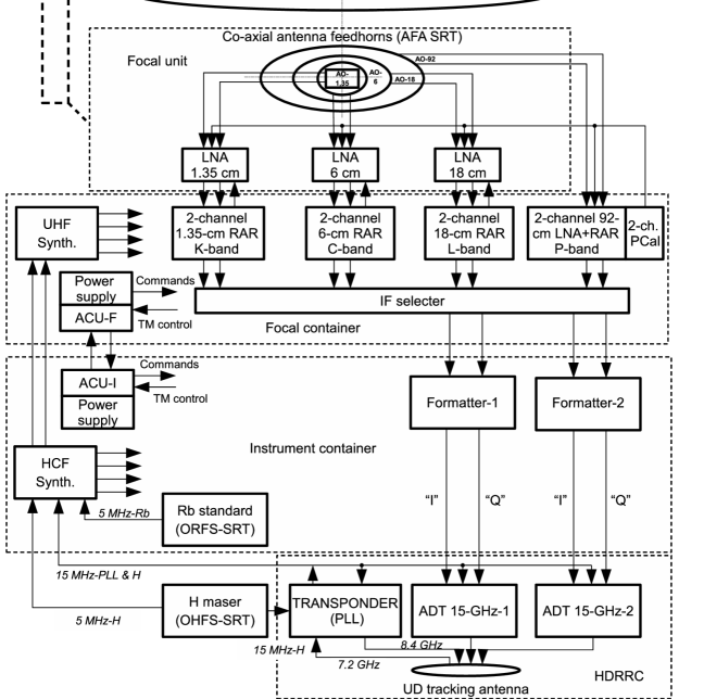
Figure 2: General block schematic of the SRT. LNA represents a low-noise amplifier; FM TRS, the focal-module thermal-regulation system; RAR, a radio-astronomy receiver; PCal, the pulsed phase-calibration block; IF, an intermediate frequency; TM, telemetry; Rb standard, the rubidium frequency standard; H maser, the onboard hydrogen frequency standard (two copies); HCF Synth., the heterodyne and clock frequency synthesizer; UHF Synth., the heterodyne ultra-high frequency synthesizer; ACU-F and ACU-I, the analysis and control units for the focal and instrument containers, respectively; HDRRC, the high-data-rate radio complex; PLL, the phase link loop; I and Q, the interferometric data fluxes in these Stokes parameters; ADT 15-GHz-1 and 2, the astronomical data transmitters at 15 GHz; UD tracking antenna, the two-dish, unidirectional, 1.5-m HDRRC antenna.

The first onboard receivers began to be delivered to the ASC in the early 1990s. Ground radio-astronomical tests of the SRT were carried out at the PRAO in 2003–2004 (see Fig. 4b in the color insert), and acceptance tests of the entire onboard complex of scientific and service instruments together with the spacecraft were conducted in 2009–2011. A functional schematic of the onboard science complex is presented in Fig. 2.

The science complex consists of the following instruments and blocks, located in the corresponding modules, shown in Figs. 1 and 2.

1. The block of co-axial antenna feeds operating at the radio-astronomy bands 1.35, 6.2, 18, and 92 cm in right- and left-circular polarizations is located in the thermally stabilized, cooled focal unit of the focal module, together with the LNA blocks for the 1.35, 6.2, and 18-cm receivers.

2. The radio-astronomy receivers operating at the four wavelengths indicated above, for both incident polarizations (denoted RAR in Fig. 2; with individual sources of secondary electric power) are located in the thermally stablized, hermetic focal container. The 92-cm LNA is located inside the 92-cm receiver. Structurally, the 92-cm receiver is joined to the block containing the pulse phase calibration units for all the receiver wavelengths. The output signals of the receivers at the intermediate frequency (IF) arrive at the IF selecter, which patches the output IF signals to the corresponding input frequency converters of the formatter for further conversion to lower frequencies. The focal container also houses a frequency synthesizer, consisting of two heterodyne ultra-high frequency synthesizer blocks (UHF Synth-1 and 2) with their sources of secondary electrical power and two analysis and control units (ACU-F) with a power-switching unit (Fig. 2).

3. Two onboard hydrogen frequency standards (OHFSs; H maser in Fig. 2) and the (scientific) instrument container are installed in the instrument module. Two onboard rubidium frequency standards (ORFS; Rb standard in Fig. 2), a frequency synthesizer with a double block forming the heterodyne and clock frequency synthesizer (HCF Synth.) and two associated power sources, two analog–digital converters for the signals from the formatter block, and the two analysis and control units of the scientific container (ACU-I) with their power supplies are housed in the thermally stable, hermetic scientific container.

The Spektr-R spacecraft with the SRT onboard is a unique piece of space science instrumentation. The entire complex of onboard equipment and the telescope are designed for a single task: multi-frequency observations of very weak radio emission at centimeter and decimeter wavelengths located far below the intrinsic noise levels of the receiver systems, and the multi-stage conversion of these signals with the very highest available phase stability into a videoband from 0 to 16 MHz, providing high-speed recording and transmission of the onboard data on the Earth. To successfully carry out this task, all instruments along the “onboard receiver–frequency converter–onboard transmitter–ground receiver station” serial line must function faultlessly, since the loss of signal or phase stability for even one of these elements (not to mention the possible failure of an element) leads to a loss of all information and a loss of very expensive observing time for all the radio telescopes forming the multi-antenna ground–space radio interferometer. For this reason, all the units and instruments have backup copies, so that there is functional redundancy in the onboard science complex, making it possible to compose this serial line of a large number of combinations of instruments and units. All this appreciably enhances the reliability of the operation of the complex as a whole. A positive effect of this approach was already exhibited during the inflight tests of the SRT: only one of the two onboard hydrogen masers tested in flight proved to have the required characteristics. This unit has been functioning continuously in orbit for more than a year.

2.2.1. Antenna Feed Assembly. The antenna-feed assembly (AFA) has a special construction, and is installed at the focus of the antenna dish. It consists of four co-axial feeds (one inside the other), in accordance with the wavelengths of the receivers. The 1.35, 6.2, and 18-cm feeds are cooled to about 150 K by a passive cooling system (see Section 2.1). These feeds are connected to the cooled LNA blocks by co-axial cables (waveguides for 1.35 cm), which also provide thermal contact between the feeds and the cold plate. The 92-cm feed is not cooled, and is at the temperature of the ambient space; it is thermally isolated from the cooled feeds to reduce the heat flow from the 92-cm to the other feeds. The 6.2, 18 and 92-cm feeds are resonance “traveling wave” feeds, with the signals divided into right- and left-circular polarizations along co-axial outputs. The 1.35-cm feed forms the open end of a waveguide with a circular apeture, with a circular-polarization splitter that makes a transition into two rectangular waveguides at the output.

2.2.2. Receiver Complex. This complex consists of onboard receivers operating at four wavelengths:

– P band, with a central frequency of 324 MHz and a ${\pm}7$ MHz bandwidth, receiver P-SRT-92,

– L band, with a central frequency of 1664 MHz and a ${\pm}30$ MHz bandwidth, receiver P-SRT-18,

– C band, with a central frequency of 4832 MHz and a ${\pm}55$ MHz bandwidth, receiver P-SRT-6M,

– K band, with a central frequency of 22 232 MHz, together with seven sub-bands for multi-frequency synthesis [30, 31], covering the frequency range 18 372–25 120 MHz, receiver P-SRT-1.35M.

The frequencies for the eight K-band sub-bands with widths of ${\pm}75$ MHz each for multi-frequency synthesis have the following names and central frequencies, separated by 960 MHz: $F_{-4}$ is 18 392 MHz, $F_{-3}$ is 19 352 MHz, $F_{-2}$ is 20 312 MHz, $F_{-1}$ is 21 272 MHz, $F_{0}$ is 22 232 MHz, $F_{1}$ is 23 192 MHz, $F_{2}$ is 24 152 MHz, and $F_{3}$ is 25 112 MHz. In addition, four sub-bands can be formed for spectral observations of narrow radio lines, with the central frequencies 22 232 MHz, 22 200 MHz, 22 168 MHz and 22 136 MHz.

All the receivers are designed to amplify, filter, and convert the noise signals and the continuous spectrum of the indicated bands into output signals at intermediate frequencies in the interval approximately from 405 to 555 MHz, and for the narrow-line signals into output signals at intermediate frequencies near 400 MHz. Each of the receivers consists of two independent, identical channels labeled 1 and 2, whose inputs are the left- and right-circularly polarized signals from the antenna-feed assembly. These channels are separated into three separate blocks: the LNA block, the receiver block, and the power-supply block. For backup of the power-supply block, channels 1 and 2 can be connected to either their own channel (1 or 2, under the command DIRECT), or to the other receiver channel (2 or 1, under the command CROSS). Both channels for the 1.35-cm receiver are supplied from the main or backup power supplies, chosen by an external command. The LNAs for L, C, and K bands are separate from the receivers, and are arranged on the cold plate in the focal unit of the radio telescope (Figs. 1 and 2), where they are radiatively cooled to temperatures $130\pm 20$ K. All the receiver and associated power-supply blocks are located in the hermetic, thermostatically regulated focal container at temperatures from ${+}5^{\circ}$C to ${+}35^{\circ}$C. The P-band LNA is located in the thermostatically controlled receiver block, at a temperature of ${+}30^{\circ}\pm 3^{\circ}$C. The construction of the P, L, and C-band receivers is based on the same design with a single frequency conversion, while the K-band receiver has two frequency conversions. The central frequency of the intermediate frequencies at L and C bands is 512 MHz, and at P band 524 MHz. The paths of the output intermediate frequencies of all receiver channels include a step attenuator, which introduces an attenuation of 0–31 dB to establish the required levels of the output signals at the intermediate frequency during the ground tests and observations in space.

In addition to the output signal at the intermediate frequency, which is fed to the IF selecter and is used further in the interferometric regime, there are two radiometric signals with amplitudes from 0–6 dB in each of the orthogonal polarizations at the receiver output, which are detected by a square-law detector at the intermediate frequency: an analog signal (converted into an 8-bit signal by the housekeeping telemetry system for transmission to the Earth) and a digital signal (12 bit). The transmission bandwidths of the radiometric paths to the detectors at the minus 3 dB level are equal to 14, 60, 110, and 150 MHz at P, L, C, and K bands, respectively; the signal-averaging time depends on the band, and is about 1 s. The bandwidth allocated from the IF output signal of the receiver for use in the interferometric regime is formed in the formatter (see below); this bandwidth depends on the observing band, and comprises from 4 to 32 MHz (two sub-bands, upper and lower, of 16 MHz each).

In each polarization channel, there is a two-level calibration noise generator for amplitude calibration, whose signal is summed with the external phase-calibration signal from the pulsed phase-calibration block, which is located in the P-band receiver and is fed to the input of the LNA block, providing calibration of both receiver channels simultaneously. The high level of the noise generator is close to the noise temperature of the channel, and is used in antenna measurements. The low level of the noise generator (which is a factor of ten lower) is used for calibration during observations of weak radio sources. The pulsed periodic signal used for the phase calibration, whose repetition frequency is 1 MHz, is used during observations in the interferometric regime. A thermostatic control system is used to enhance the stability of the amplification and the signal level of the noise generator. The receiver blocks and noise-generator blocks within them are separately thermostatically regulated, and the LNA blocks exposed to open space are likewise thermally stabilized. The temperatures are monitored through the telemetry parameters.

2.2.3. Onboard Frequency Standards. Frequency (phase) stability is of key importance in VLBI, and is determined in first instance by the frequency standard used, whose signal acts as a primary reference signal for realizing the necessary subsequent frequency conversions. The SRT is designed to function with reference signals from three sources: 1) the onboard hydrogen frequency standard (OHFS; 5 MHz or 15 MHz), 2) the 15-MHz signal of the phase-synchronization loop of the high-data-rate radio complex (HDRRC), which is synchronized by the signal from a ground hydrogen maser at the tracking station, and 3) the onboard rubidium frequency standard (ORFS; 5 MHz).

A hydrogen maser device was launched vertically in a rocket to a height of 10 000 km and successfully operated during two hours of flight in 1976. Its purpose was to measure the gravitational potential and test the predictions of relativistic gravitational theory as part of the Gravity Probe A experiment [32]. The European Space Agency launched the GIOVE-B navigational satellite with three atomic clocks on board into Earth orbit in 2008; a passive hydrogen maser was used as a primary reference, and two rubidium oscillators as secondary references [33]. The RadioAstron onboard hydrogen maser is the first active onboard hydrogen frequency standard in a near-Earth orbit, and has now successfully been used to realize the orbital program for more than a year. Therefore, the results of its inflight tests as part of the SRT have special value, both scientifically and practically. A number of specialized problems not usual for maser frequency standards were solved during its construction at the Vremya-Ch Joint Stock Company:

– degassing of the thermostats by the vacuum of space;

– the need to enhance the structural stability of the resonator and storage bulb for the hard conditions to which the instruments are subject during launch;

– temperature stabilization of the standard using the system for thermal regulation of the instrument base, and thermal isolation of the structure of the OHFS using multi-layer vacuum insulation;

– carrying out ground tests in the absence of the vacuum of space;

– a number of engineering problems associated with the use of instruments in the vacuum of space.

In addition, new problems arose, associated with the higher stability of the onboard masers and the appearance of new destabilizing factors in space flight, such as the gravitational and relativistic shifts of the standard frequency due to the motion of the spacecraft in its orbit. Since this is the first experience using a hydrogen maser under such unusual conditions, other unforeseen problems are also likely to appear.

2.2.4. Reference-Frequency Generator. The secondary reference frequencies are generated in the heterodyne and clock frequency generation blocks, and the heterodyne ultra-high frequencies in the corresponding HUHF blocks (Fig. 2). The HCF blocks form the 64 and 160 MHz secondary reference signals, 72-MHz clock-frequency signals, and 40 kHz synch-frequency signals required for the functioning of the instruments in the science complex, based on the primary reference signals at 5 MHz or 15 MHz from the OHFS or the 15 MHz signal from the loop phase link (which will be discussed below). The HUHF block is a functional continuation of the HCF block, and is conceptually similar. The heterodyne signals for the 92-cm (at 200 MHz), 18-cm (at 1152 MHz), and 6.2-cm (at 4320 MHz) receivers, and also the 8-MHz reference signals for the formation of the heterodynes inside the 1.35-cm receiver and for the pulsed phase-calibration block inside the 92-cm receiver, are formed from the secondary reference signals from the HCF and HUHF blocks. This calibration is realized for all the receivers at intermediate frequencies. The frequency-generation system of the SRT is described in more detail in [34].

2.2.5. Intermediate-Frequency Selector. The IF selecter patches any IF outputs from the receivers (four outputs in each of left- and right-circular polarization) to any two inputs of the main or reserve formatter block (Fig. 2), apart from combinations of the same polarization in different ranges (left with left, right with right). The configuration is specified by the selecter keys, which are established by external commands. In single-frequency mode, signals from one or two IF outputs from the receivers of a specified frequency can be patched to the formatter — in left- and/or right-circular polarization. The signal from any one IF output can be patched to two inputs of the formatter in parallel, which is important during test measurements. In two-frequency mode, two IF signals from the receiver outputs for any two frequencies can be patched to the formatter, but with the restriction indicated above concerning combinations of the same polarization at the different frequencies.

2.2.6. Formatter. The formatter

– converts the signal spectrum from the receiver output from the IF frequency range to the videofrequency range, and forms the upper and lower sidebands of the videospectrum from 0 to 16 MHz each (SSB videoconverter);

– carries out the conversion for transmitting the videodata to the Earth via the onboard high-data-rate radio transmitter at 15 GHz.

The separation of the upper and lower sidebands of the videospectrum is carried out according to a SSB-converter scheme with rotations of the signal phases by $90^{\circ}$, $180^{\circ}$, and $270^{\circ}$, as is required for reliable formation of the sidebands. The videosignals are converted into digital form, and are digitally filtered using a seventh-order Butterworth filter. The use of digital filters ensured high repeatability of the shape of the amplitude–frequency and phase–frequency characteristics. Filter bandwidths of 4 MHz or 16 MHz can be chosen.

The conversion chain for the transmission of the signals to the Earth includes:

– the one-bit (two-level) clipped videosignal and its conversion to digital form;

– the parallel, synchronous interrogation of the digital values of the signals in the upper and lower sidebands;

– conversion of the parallel sub-streams of data into a denser serial, high-data-rate stream;

– the generation of the frame structure of the high-data-rate stream of the synchronized, serial streams and introduction of the data from the onboard telemetry system into the frame headers;

– execution of differential coding of the signals for equalization of the phase-modulated signal spectrum transmitted through the HDRRC channel.

The result of interrogating the signal values for a single sideband is a stream with a data rate of $16\times 2=32$ Mbits/s or $4\times 2=8$ Mbits/s for a video bandwidth of 16 or 4 MHz, respectively. To transmit the entire volume of information (four videobands) with a serial stream, taking into account the introduction of a ninth parity bit for each transmitted byte of information, the data rate is $32\times 4\times(9/8)=144$ MHz and $8\times 4\times(9/8)=36$ MHz for video bandwidths of 16 and 4 MHz, respectively.

Two IF converters are provided in the formatter system. The digital information taken from them arrives at the data stream of the corresponding converter at the high-data-rate stream generator. Note that the videodata are transferred through the high-data-rate channel using a transmitter with quadrature phase manipulation of the carrier frequency of 15 GHz. This makes it possible to simultaneously transmit two characters of information, which is used in this instrument. Therefore, the clock frequency of the serial data stream can be lowered by a factor of two, so that it comprises 72 and 18 MHz for video bandwidths of 16 and 4 MHz, respectively. Differential coding is provided to improve the energetic parameters of the video-data transmission line in the instrument. As a result, two streams of digital information are obtained at the output of the instrument after the coding, but with “mixed” data from the two streams from the converters. These streams are denoted I and Q, and arrive at the modulator of the 15-GHz transmitter of the HDRRC.

The I and Q streams are divided into frames with durations of 2.5 ms and 10 ms for the clock frequencies of 72 MHz and 18 MHz, respectively. Within a frame, the information is transmitted in bytes. A ninth parity bit is created for each 8 bits, which is transmitted in the data stream. The bits are rigidly fixed to the source of data, so that they can be identified and sorted according to the corresponding groups after the arrival of the stream at the Earth (to reconstruct the sub-streams of the onboard formatter).

For housekeeping purposes, the first 30 bytes in a frame are formed as a header, which includes a synchronization packet of seven bytes (for precise determination of the times for the 1st bit and 1st byte of the frame and the subsequent correct decoding of the binary data), a frame counter (2 bytes) from the 1st to the 400th frames, and the bytes of certain accompanying information. The first 10 bytes of the header are used to transmit telemetry information from the standard onboard telemetry system, which is especially important in the observing regime with the housekeeping telemetry channel for command–measurement information turned on (see below). The operational mode for the converter is chosen using commands transmitted to the instrument along the address bus using control code words (CCWs).

2.2.7. Analysis and Control Units. The onboard science complex is controlled mainly through the ACU-I and ACU-F instuments, using pulsed functional (PF) commands and CCWs. In the ACUs, the digital CCW commands are converted into commands analogous to pulsed commands. Some instruments (the OHFS, P-SRT-1.35, and P-SRT-Rec) are controlled directly by CCW commands sent along the address bus.

Monitoring of the functioning of the complex instruments is carried out using the standard onboard telemetry system. Telemetry signals arrive at this system directly from the instruments or via the ACU collection system, in accordance with the requirements of the apparatus. Some of the telemetry data are generated in the form of digital databases (for example, some of the data from the 1.35 cm receiver and all the data from the OHFS are telemetrized in this say).

Currently, the onboard science-equipment complex is providing full functioning of the SRT in essentially all operational modes, thanks to the system of functional and instrumental duplication. Most of the duplicated instruments are located in reserve, as a contingency.

2.3 Ground Tests

During preparations for the Spektr-R launch, various tests were carried out at the ASC in accordance with the requirements for the scientific equipment to be used. At early stages in the construction of the SRT, the goal of such tests was to achieve the required technical specifications for the parameters of individual instruments. Later tests of the onboard science-equipment complex and the spacecraft were designed to determine the capabilities for their joint operation in flight.

Starting from the mid-1990s, after the first sets of instruments were delivered, tests of their electrical coupling and electromagnetic compatibility were carried out at the ASC. The programs and methods for the tests were developed as they proceeded, and the functional adequacy of the instruments and the completeness of the complex of scientific equipment was determined. Three integrated tests based on a zero-baseline interferometer were carried out in 1999–2002, during which specific parameters of the interferometer were obtained and compared with calculated values. A set of receiving equipment designed for ground radio telescopes was used as the second element of the interferometer. By the second half of 2002, the entire radio complex was technologically ready to conduct radio-astronomical tests at a specially built test facility at the PRAO.

2.3.1. Radio-Astronomy Tests. The SRT was assembled at this test facility on a support structure in 2002–2003. The dish surface was geodetically adjusted, the electrical assembly of the science-equipment complex and ground equipment carried out, and the entire complex and test facility functionally checked. From the end of 2003 through mid-2004, radio-astronomical tests of the engineering model of the SRT were carried out using actual astronomical sources (see Fig. 4b in the color insert).

Fluctuations of the sensitivity of the system, the effective area of the SRT, and the width and shape of the main lobe of the antenna beam were measured in the radiometric regime. The positions of the first sidelobes and the level of scattering outside the main lobe of the antenna beam were determined (including using observations of the Moon); see Table 2 in Section 5. The focal container of the radio telescope was adjusted to determine the position of the focus relative to the calculated value, and the difference between the positions of the geometrical and electrical axes of the SRT was determined.

Observations of astronomical sources for tests of the SRT in a radio-interferometric regime were conducted at 6.2 and 1.35 cm using the PRAO 22-m radio telescope as a second interferometer element. This same two-element interferometer was used to investigate the interference environment at all the operational wavelengths of the SRT, and the possibility of transmitting reference signals from a hydrogen maser. The electromagnetic compatibility of the 1.35-cm receiver and the 15-GHz HDRRC transmitter was investigated, and individual elements of the tracking station were tested, in particular, the S2 and RadioAstron data recorders and the ASC–NRAO decorder.

Although the results of these tests led to difficult decisions about changing the formatter, antenna-feed assembly, and decoder and the need to further develop the ACUs and RadioAstron data recorders, the main result of the tests was that the ASC obtained an operational radio-electronical complex, i.e., a full set of scientific equipment, for further study.

2.3.2. Zero-Baseline Interferometer Tests. After completion of the radio-astronomical tests, the SRT was disassembled and the entire engineering model of the science-equipment complex was sent to the ASC for further zero-baseline interferometer tests. This stage of the testing was continued during 2005–2008, and the tests were carried out at 6 cm. The first task of these tests was the practical verification of the compatibility of the scientific data obtained by the space and ground radio telescopes. This task was successfully completed in full. The second task was comparison of the interferometer parameters measured through a data-correlation analysis with their calculated values. The results of the comparison were satisfactory, and provided reliable experimental material for determining the interferometer sensitivity and the required coherence time for the integrated signal.

In mid-2008, a flight model of the onboard science complex was delivered to the ASC for use in zero-baseline interferometer tests. Tests at 6.2 and 1.35 cm were conducted using this model, but with new onboard P-SRT-6M and P-SRT-1.35M receivers. The results of these tests showed not only a good agreement between the calculated and experimental parameter values, but also stability of these values both in time and for different models. Based on these test results, and taking into account the dual-channel design of the onboard receivers, it was decided to simplify and shorten further tests due to the subsequent unavailability of the ground scientific equipment. The interchannel correlation function obtained during the correlation reduction of signals that had passed through corresponding pairs of receiver channels was adopted as a key parameter estimating the operation of the onboard science complex. Further, when conducting various grades of factory tests at the Lavochkin Association, the interchannel correlation function was used as the main parameter characterizing the state of the onboard science complex.

This essentially completed the radio-engineering tests of the SRT equipment at the ASC. The suitability of the apparatus for radio interferometric observations and its full radio-engineering compatibility was demonstrated.

At the beginning of 2009, the flight model of the onboard science complex of the SRT was sent to the Lavochkin Association for the final assembly and integrated and acceptance factory tests of the SRT complex. The assembly of the entire SRT took place in 2010–2011, together with integrated factory tests and acceptance tests of the SRT complex. The complex was mounted on the Navigator service module in April–June 2011, and integrated tests of the Spektr-R spacecraft were successfully completed. Although these were electrical tests of the SRT complex, in the interests of verifying the future joint functioning of the scientific equipment and the service module in flight, the interchannel correlation function was continuously monitored during these tests. The fully assembled launch vehicle and Spektr-R spacecraft were transported to the launch position in July 2011, and the Spektr-R spacecraft was successfully launched on July 18, 2011. In the following sections, we present material on inflight tests of the SRT and the transition to the main science program.

2.4 SRT–Ground High-Data-Rate Radio Line

The high-data-rate radio line includes the onboard HDRRC and the ground tracking station, together with the scientific data collected using the PRAO 22-m radio telescope in Pushchino.

2.4.1. HDC Onboard Complex. The onboard HDRRC is designed to transmit data from the SRT to the ground tracking station at a high rate, and to synchronize the onboard reference frequency using a signal from a ground hydrogen maser in one of the operational regimes of the SRT and the HDRRC. The HDRRC can operate in one of two regimes: “COHERENT” or “H maser”.

In the “COHERENT” regime, the HDRRC is used to synchronize the 15-MHz onboard reference signal for the SRT frequency-generation system, as well as the HDRRC transmitter signals at 8.4 GHz (a power of 2 W) and 15 GHz (a power of 40 W). This is done using a hydrogen-maser signal that is transmitted to the spacecraft from the ground tracking station. In the “H maser” regime, the 15-MHz HDRRC transmitter signals are synchronized using a signal from the onboard hydrogen maser. It is possible for the HDRRC to operate with a lower transmitter power output (4 W) at 15 GHz.

The HDRRC includes the antenna-feeder system and onboard radio-engineering complex. The antenna-feeder system includes:

– a double-reflector, receiving–transmitting, narrow-beam antenna with a diameter of the primary reflector of 1.5 m;

– a rotating waveguide junction joined to the drive of this antenna; and

– a waveguide tract and filters.

The onboard HDRRC radio-engineering complex contains:

– a transponder phase-synchronization loop at 7.2/8.4 GHz;

– a radio transmitter at 15 GHz.

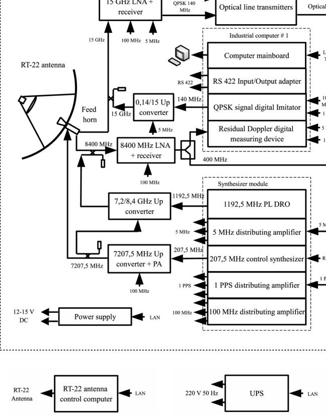
Figure 3: Stuctural schematic of the ground tracking station in Pushchino.

2.4.2. Ground Tracking and Scientific Data Acquisition Station. The ground tracking and scientific-data-acquisition station is part of the high-data-rate SRT–ground radio link of the RadioAstron project. A structural diagram of the tracking station is presented in Fig. 3. The station is designed to

1) point the PRAO 22-m ground radio telescope toward the SRT and track the spacecraft during a link session;

2) receive and record the flow of scientific and housekeeping data from the spacecraft;

3) transmit a phase-stable reference signal synchronized by a ground hydrogen frequency standard (the tracking station H maser) to the spacecraft;

4) receive the response signal coherently converted onboard the spacecraft, measure the current frequency of the residual Doppler shift and the current phase difference between the response and interrogation signals, and record these measurements with a current time tag;

5) receive the external data required for the operation of the ground station and issue information about the status of the ground tracking station and the data collection to users.

The ground tracking station includes:

– the PRAO 22-m radio antenna, pointing system, feedhorn, and antenna-feeder tracts at 15, 8.4, and 7.2 GHz;

– the phase-synchronization transponder system at 7.2/8.4 GHz;

– the system for the reception of scientific and housekeeping data at 15 GHz;

– the system for measuring the Doppler residual and variations in the HDRRC signal phases;

– the system for recording the scientific and housekeeping data;

– the system for the reference frequencies, time service, and weather station;

– the control computer and station software;

– the apparatus for monitoring the operation of the station;

– the apparatus for external links and the cable-distribution network.

The effective area of the 22-m antenna with the tracking-station antenna-feeder system and the receiver system noise temperature were measured. The measured effective area of the 22-m antenna is 170 m² at 15 GHz. The system noise temperature is about 100 K at both 8.4 and 15 GHz.

Apparatus for Measuring the Frequency Doppler Shift. The operation of the ground tracking station’s system for measuring the frequency Doppler shift was tested during the inflight tests. Since these measurements are carried out at each of the downlink frequencies of 8.5 and 15 GHz, there are two such measuring systems at the station. The 8.4-GHz measuring device operates using a tone signal emitted by the onboard HDRRC phase-synchronization loop, while the 15-GHz measuring device operates using a phase-modulated signal (produced using the “quadrature phase manipulation” method) emitted by the HDRRC VLBI-data transmitter. During these tests, these signals were fed to the inputs of the Doppler-shift measurement device and sent to the screen of a spectrum analyzer in parallel, which was used to carry out independent measurements of the frequency, signal-to-noise ratio, and other parameters of the input signals. The 8.4-GHz Doppler-shift measurement device can operate in one of three regimes:

1) “Without control”: the frequencies of the downlink, Doppler residual, and integrated phase are measured; the uplink signal from the ground tracking station is not transmitted; the ballistic-software data are used only to obtain the Doppler residual; used in the “H-maser” regime of the HDRRC;

2) “Ballistical”: data from a ballistic file (the delay and its first and second derivatives) are used to control the uplink frequency; measurements of the downlink frequency, Doppler residual, and integrated phase are recorded; used with the “Coherent-B” regime of the HDRRC;

3) “Autonomous”: used for independent control of the uplink frequency based on measurements of the downlink frequency, Doppler residual, and integrated phase; the ballistic data are used only to obtain the initial delay; used with the“Coherent-A” regime of the HDRRC.

The 15-GHz measuring device always operates only in the “without control” regime, measuring and recording the frequencies of the downlink, Doppler residual, and integrated phase. The RefFreq program controlling the measuring device was used to verify the operation of this device at 8.4 GHz. Analogous verification was carried out for the measuring device at 15 GHz using the RefFreqM program. The test results confirmed the full operability of the measuring devices at 8.4 GHz and 15 GHz and their software in all operational regimes.

Apparatus for the Reception of Scientific Video and Telemetry Information. This apparatus includes instruments in the channels for the reception of scientific video and telemetry (TM) information. The former consists of the science data decoder and the RadioAstron data recorder (RDR). The science data decoder extracts the useful signal from the data flow arriving at the decoder from the science data demodulator (the scientific data are subject to a special form of phase modulation onboard). The science data decoder also decodes and operatively monitors its input data. The data recorder writes the scientific data in the operational mode. The start of each recording is synchronized by short pulses with a period of 1 s using a 5-MHz reference signal from a hydrogen maser at the ground tracking station. The duration of a recording is six to nine hours at the highest recording speed. The recorder is controlled either directly or via an Ethernet channel with remote access. The data recorder at the ground station is used together with control software.

The apparatus in the channel for the reception of telemetry data includes a decoder for the specialized telemetry data (10 bytes at the beginning of the frame headers) from a dedicated data-transmission line at the Flight Control Center (FCC) of the Lavochkin Association sent from the tracking station in Pushchino. The TM data decoder extracts from each frame of the HDRRC the 10 bytes of telemetry data from the standard telemetry system of the spacecraft, and saves this information to a hard disk and/or directly transmits the telemetry data to the FCC or the ASC via an Ethernet port.

Experience has been obtained with the reception, decoding, and transmission of telemetry data from the spacecraft to the FCC during scientific and test observations. In all scientific SRT–ground link sessions, the frequency and Doppler residual were measured at 8.4 and 15 GHz along the HRCRC channel to the tracking station in Pushchino. These measurements were then fed to an ftp server at the ASC data-reduction center for further processing and analysis.

Studies of the operation of the high-data-rate radio line, consisting of the HDRRC complex and the tracking station, were carried out during link sessions between the spacecraft and the ground tracking session, both with the SRT operating as a single dish and as an element of a multi-antenna radio interferometer together with ground radio telescopes. To enhance the level of the signal arriving at the Earth, the program used to point the onboard HDRRC antenna toward the 22-m ground radio telescope in Pushchino was refined. The agreement of the polarizations of the onboard HDRRC antenna and the antenna-feeder system of the 22-m telescope in the 15-GHz receiver channel was verified and corrected, leading to an increase in the received power by nearly a factor of ten. The high potential of the radio line providing stable operation of the entire complex in Pushchino was confirmed for various distances of the spacecraft in its orbit. At relatively nearby distances (less than 150 000–200 000 km), the transmitter power is chosen to be 4 W, while this power is increased to 40 W at greater distances. The connections between the ground station, the Lavochkin FCC, and the Ballistic Center, Science Scheduling Center, and Science Data Reduction Center (SDRC) of the ASC have all been debugged.

3 LAUNCH, INFLIGHT TESTS OF SPEKTR-R AND THE GROUND CONTROL COMPLEX

The RadioAstron Spektr-R spacecraft was launched from the Baikonur cosmodrome on July 18, 2011 at $05:31:17.91$. The spacecraft was inserted into its orbit using a Zenit 2SB.80 rocket and a Fregat-SB booster, and the sequence of activities for the first session was realized (Figs. 4, 5).

The scheme for introducing the spacecraft [21] into its orbit (with a perigee height 577 km, apogee height $h_{a}=336\,863$ km, and orbital inclination $i=51.6^{\circ}$) included successive transfers to a supporting orbit ($h_{p}=177$ km, $h_{a}=447$ km, $i=51.4^{\circ}$) and an intermediate orbit ($h_{p}=444$ km, $h_{a}=3711$ km, $i=51.5^{\circ}$). The control of the Spektr-R spacecraft is carried out by the FCC of the Lavochkin Association.

The Spektr-R spacecraft was constructed at the Lavochkin Association, based on the Navigator space platform [21, 24], which was successfully developed for the Elektro-L spacecraft launched at the beginning of 2011. The Spektr-R spacecraft is controlled by the Main Operations Control Group (MOCG) at the Lavochkin Association, with the participation of specialists from the organizations that developed the onboard systems and, in particular, the onboard science complex, ground control segment, and ground science complex. The principles for the organization of the work of the MOCG are those traditional for the Lavochkin Association. The control and analysis groups include specialists from the Spacecraft Logic and Control Division who participated in the planning of the spacecraft and its ground tests, and also in the preparation and tests of the ground segment for control of the spacecraft. The staff of the analysis group includes specialists of the Special Design Bureau supervising the corresponding onboard systems, who were also involved in all stages of planning and testing of these systems. Specialists from the Lavochkin Association also make up the Ground-Segment Control Group, Ballistic Group, FCC Instrument and Software Group, and GS-3.7 Ground-Station Group at the Lavochkin Association. The MOCG also functions as:

– the Science Operations Group for the Science Scheduling Center of the ASC,

– the Science Operations Group of IKI for the Plazma-F project,

– the Technical Operations Group for the SDRC,

– the Technical Operations Group for monitoring of the data-conversion block.

The reduction of measurements of the orbital parameters and reconstruction and prediction of the spacecraft orbit are carried out by the Technical Operations Group of the Ballistic Center of the IAM, with the participation of specialists from the Lavochkin Association.

The operation of the MOCG began long before the launch of the spacecraft, and included preparing the apparatus and software facilities of the FCC, the spacecraft control software, operational and technical documentation, training of personnel, conducting autonomous and integrated tests of the ground control segment, debugging the connections between the FCC facilities and the control stations and ground science complex, and conducting practice sessions for the Control Group. This approach to the formation of a main control group, traditional for the Lavochkin Association, which also organizes preparation of personnel and the apparatus and software facilities enabled the preparedness and reliable control of the Spektr-R spacecraft from the very first days of flight.

One special characteristic of the organization of the operation of the RadioAstron ground–space interferometer is the need to coordinate the actions of the SRT, ground radio telescopes, the ground tracking stations, stations for command and control of the spacecraft, the FCC, the Science Scheduling Center, the Ballistic Center, and science-data reduction centers, including facilities for communication between these elements. The main task in the current stage of the project is carrying out a program of science observations during a number of science sessions. As a rule, an observing session lasts several hours, but the duration can be days or more in some cases. A session corresponds to a series of operations providing recording of the data from an observed source, conversion of the signals obtained into digital form, transmission of these data to the ground tracking station, and collection of the scientific data. The scientific data are transmitted to the ground tracking station via the high-data-rate radio channel in the Ku band (2 cm) and an onboard narrow-beam, 1.5-m antenna, which is controlled from the onboard control complex. The Spektr-R spacecraft is able to operate with several ground tracking stations. As was noted above, the station that is currently used for tracking and scientific-data acquisition is the PRAO 22-m radio telescope of the ASC.

A target source is observed with a network of ground radio telescopes simultaneously with the SRT. Several dozen radio telescopes have equipment that is compatible with that of the Spektr-R SRT, and can in principle participation in joint VLBI observations. The participation of these observations is determined in part by the requirements of the specific science projects to be carried out.

The command and control ground stations used with the spacecraft include the “Kobal’t-R” station at Bear Lakes (Moscow region), which has a TNA-1500 antenna complex (Moscow Energy Institute) and an antenna with a 64-m diameter, and “Klen-D” (Ussuriisk), which has a P-2500 antenna complex and a 70-m-diameter antenna. The mean command-session duration is about four hours. In accordance with a decision by the control group, as a rule, the onboard command-measurement system transmitter is not turned off at the end of a session, in order to make it easier to enter into the new link in the following session. However, this transmitter is turned off during intervals when the science receivers of the SRT are switched on, i.e., during tests and science observations. When turned on, the transmitter can also be used to monitor the telemetry information from the spacecraft at distances to 120 000 km (near perigee) using the Lavochkin NS-3.7 ground station with its 3.7-m-diameter antenna.

The typical program for a control session consists of the following operations:

– monitoring the current housekeeping information as it is being directly transmitted;

– uploading of command sequences for the spacecraft systems for flight and attitude control, control of the antennas and telemetry system, control of the onboard command complex, entering command sequences for ballistic and navigational use (roughly once in five days), and uploading individual code commands either directly or with a time lag;

– monitoring telemetry information recalled from onboard memory and the electrostatic control system;

– monitoring of the spacecraft orbit;

– unloading of the attitude-control reaction wheels;

– playback of the scientific telemetry information from the science-data collection system of the Plazma-F complex;

– uploading of the command sequences for control of the Plazma-F science-apparatus complex.

During a command and control session, an operational program enabling the following tasks of a typical operational cycle in an autonomous regime is uploaded in the form of command sequence.

1. Conducting an observing session consisting of the following individual operations:

– successive rotations of the spacecraft into a specified attitude, enabling pointing of the SRT toward a target and pointing of the HDRRC narrow-beam 1.5-m antenna toward the ground tracking station in Pushchino;

– turning on the required operational regimes of the SRT instrumentation at the observation time;

– reverse rotations of the spacecraft to its original attitude.

2. Radio-adjustment of the SRT:

– operations analogous to an observing session, but with the realization of a series of successive reorientations of the spacecraft relative to the direction toward a calibrator radio source without pointing of the HDRRC antenna at the Pushchino tracking station (the SRT information is written to an onboard memory unit and recalled at the following control session).

If the required spacecraft attitude is expected to lead to a worsening of the temperature regime of the structural elements of the HDRRC complex (girders, antenna drive, transmitter), the HDRRC antenna can be moved to the position corresponding to the position of the Sun on the spacecraft axes.

3. Laser ranging of the spacecraft:

– reorientation of the spacecraft over an hour to the position in which the $-X$ axis of the spacecraft is oriented toward the Earth (i.e., the SRT is facing away from the Earth);

– bringing about the spacecraft attitude required for the plasma-energy monitoring instrument (MEP) from the Plazma-F complex, with the Sun located at $100^{\circ}$ to the ${+}X$ axis, for a duration of up to six hours, with movement of the HDRRC antenna to a specified position.

The sequences of operations during observations of sources, radio adjustments, and laser ranging are determined by the monthly program of scientific activities generated by the SRT Science Operations Group (ASC). This program takes into account scientific tasks, the current ballistic parameters of the orbit, the current constraints on the activities of the ground radio telescopes, and constraints on the duration of observational regimes for specified attitudes of the spacecraft, depending on the position of the Sun relative to the spacecraft axes and the position of the HDRRC antenna. The Ballistic Group for Inflight Analysis and the Thermal Regulation System (TRS) Group applies the operational-analysis software of the FCC to evaluate the realizability of the monthly science program from the point of view of all the constraints.

The TRS Group is accumulating a large amount of statistical material, which can be used to predict variations of the temperature fields in critical structural elements of the spacecraft as a function of the positions of the Sun and the HDRRC antenna with the required accuracy. Work is being carried out on the automation of required calculations for enhancing the efficiency and reliability of such predictions, and also to facilitate estimated predictions by specialists at the ASC at the stage of formulation of the monthy science program. The TRS Group uses a specially developed three-dimensional model of the spacecraft enabling visual illumination of the structural elements of the spacecraft for various positions of the Sun and the HDRRC antenna.

The Command and Control Group of the Lavochkin Association develops the monthly program for the Spektr-R spacecraft based on the monthly science program. In accordance with proposals, and the preferred intervals for the special attitude of the spacecraft required for optimal operation of the MEP instrument, the program includes additional operations on the reorientation of the spacecraft. The Spektr-R program is confirmed by the operational technical administration of the MOCG, and becomes the main document facilitating coordination of the operational work of all systems of the Spektr-R spacecraft. The program contains the schedule of sessions for the following month, the schedule of all main operations with the spacecraft, and the schedules of operation for the control stations, tracking stations, ground radio telescopes, and laser-ranging stations. The actions of the command and control stations are organized by the Ground Segment Control Group at the Lavochkin Association, of the station in Pushchino and the ground radio telescopes by the SRT Science Operations Group at the ASC, and of the laser-ranging stations by the Ballistics and Navigation Group at the IAM.

One day before the following session, the Command and Control Group develops a plan for the session, in accordance with the monthly schedule for the Spektr-R spacecraft and based on template programs. The spacecraft navigation data and data from the HDRRC antenna are analyzed by the Ballistic Analysis Instrumental–Software Control Group of the FCC. The generation of inflight specifications for the control of the SRT science-equipment complex and the Plazma-F complex is done automatically based on command-software information prepared by the SRT and Plazma-F Science Operations Groups. The session program is generated in the form of a control file containing command-software information for controlling the spacecraft and commands for controlling the ground command–measurement stations. The correctness of the program is verified using a data–logicical model for the onboard control complex, which fully corresponds to the programmatic part of the real onboard complex of the Spektr-R spacecraft. This modeling is carried out for successive time intervals, from the beginning of the session being verified to the beginning of the following planned session, for one to two days of flight.

The realization of the program for a housekeeping telemetry session occurs in an automated regime, with the commands directed toward particular instruments being obtained from the spacecraft and the command–measurement stations. During such sessions, the telemetry data from the spacecraft arriving at these stations is processed at the Lavochkin FCC, analyzed by specialists of the Analysis Group, and transferred to the SDRC of the ASC. The measurements of the orbital parameters are sent to the FCC from the command–measurement stations, and further to the IAM.

As the tasks in the program of inflight tests of the onboard systems of the spacecraft were carried out, the number of Analysis-Group specialists who were involved in routine operations was reduced. Currently, only specialists of the Complex Analysis Group, Onboard Control Complex Service, and TRS Service regularly participation in the routine monitoring of the telemetry information from the spacecraft. The telemetry analysis uses a program for the automated monitoring of important parameters of the spacecraft to ensure compliance with tolerances and with predicted values obtained in simulations of sessions using the onboard control complex model. The Onboard Systems Service is able to monitor the telemetry information outside the FCC, at its work places. Once they have received the housekeeping telemetry information from the FCC in real time, specialists in the SRT and Plazma-F Science Operations Groups at the ASC and IKI monitor the functioning of the science-equipment complex. When remarks on the operation of the complex are required during a control session, these groups request an operational delivery of additional command-software information to the address of the science-equipment complex.

Before the beginning of the entire cycle of tests with the spacecraft, a ground tracking and data-collection station was established at the 22-m radio telescope in Pushchino. The data obtained by the ground tracking station during interferometric observing sessions is also used to monitor the status of the spacecraft. The housekeeping telemetry information extracted from the headers of the science frames received by the Pushchino ground station, transmitted through the HDRRC channel, is sent on to the FCC. These data are processed and used in the same way as the telemetry data transmitted through the radio channel: through the small onboard antenna, during link sessions with the command–measurement ground stations, following observations.

The organization of the control of the Spektr-R spacecraft and of the Main Control Operations Group described above has provided operational and reliable control of the Spektr-R–RadioAstron complex, including during the earliest stage of flight, when the first series of tests were carried out. The inflight tests and organization of the control of the Spektr-R spacecraft are described in more detail in [26].

Table 1: Parameters of the RadioAstron orbit on April 14, 2012 (32 orbital revolutions after launch)

Major axis	$a=174\,714.234$ km
Eccentricity	$e=0.692$
Orbital inclination	$i=79.69^{\circ}$
Ascending node longitude	$W=300.55^{\circ}$
Argument of perigee	$w=303^{\circ}$
Time of perigee passage	07:12:37.00 UTC
	14 April, 2012
Orbital period	${\approx}8.5$ d

4 THE ORBIT: PARAMETERS, MEASUREMENTS, AND PRECISION OF RECONSTRUCTION

After the launch, the major axis of the spacecraft orbit was 173 400 km, its perigee height 578 km, its apogee height 333 500 km, and its orbital period 8.32 d. The first observations were made from this orbit. Several months after inserting the spacecraft into its operational orbit, it became clear that the useful life of the spacecraft could potentially end as early as the end of 2013, due to the low perigee of the orbit. To avoid further lowering of the orbit perigee, the system of onboard vernier thrusters was fired twice in order to correct the orbit. After this correction (March 1, 2012), the orbit has a calculated ballistic lifetime of more than nine years, with the interval when the spacecraft is shadowed by the Earth being no more than two hours. The orbital elements after correction (on April 14, 2012) are presented in Table 1.

The orbit evolves due to the perturbing influence of the Moon and Sun. The eccentricity will vary from 0.96 to 0.59 during the spacecraft’s lifetime, and the orbital inclination will vary in the range $10^{\circ}$–$85^{\circ}$. Figure 6a shows the evolution of the radii of perigee and apogee after the above correction. The radius of perigee varies from 7000 km to 81 500 km, and the radius of apogee from 280 000 to 353 000 km. Further observations of the spacecraft motion have shown that the above correction proceeded normally, and estimates of the actual parameters of the correction are close to the calculated values. Figures 6b–6e show the calculated evolution of the projected orbit in 2013–2016. Figures 6f–6k show examples of the corresponding evolution of the K-band $(u,v)$ coverage obtained for syntheses carried out over a year using the two edge sub-bands (1.19 and 1.63 cm), for 2013, 2014, and 2015, for the radio galaxy M87 (Figs. 6f–h) and Cen A (Figs. 6i–k). The region encompassed by the observations in the $(u,v)$ plane is appreciably elliptical for both sources. Therefore, an additional orbital correction may be applied in the future, in order to realize uniform filling of the $(u,v)$ plane in all directions. More detailed information about these new possibilities can be found in [35], and about the evolution of the orbit over the next five years at the project web site [25].

Figure 6: (a)–(e) Calculated time evolution of the SRT orbit and (f)–(k) examples of the $(u,v)$ coverage obtained for syntheses carried out using the two edge sub-bands $F_{3}$ (1.19) and $F_{-4}$ (1.63 cm) in the 1.35-cm band. Panel (a) shows the perigee height $P$ and apogee height $A$. Panels (b)–(e) show the coverage of the celestial sphere with possible observations with the ground–SRT interferometer in (b) 2013, (c) 2014), (d) 2015, and (e) 2016; the letters “B” and “E” denote the beginning and end of the orbital evolution over the year. Panels (f)–(h) show the $(u,v)$ coverage obtained for observations of the galaxy M87 with the SRT and the Green Bank (USA), Goldstone (USA), Effelsberg (Germany), Jodrell Bank (UK), Evpatoria (Ukraine), Parkes (Australia), Tidbinbilla (Australia), and Robledo (Spain) ground stations carried out in (f) 2013, (g) 2014, and (h) 2015; the position angle of the jet in M87 is ${-}77^{\circ}$. Panels (i)–(k) show the same as (f)–(h) for the galaxy Cen A, whose jet position angle is $51^{\circ}$). Synthesis of the broad frequency band with eight sub-bands from 1.63 to 1.19 cm leads to appreciable additional filling of the $(u,v)$ plane between the tracks shown for these edge wavelengths.

Carrying out interferometric observations requires determining the ground–SRT baseline with very high precision. The Spektr-R spacecraft is very complex from the point of view of nagivation support. One of the factors influencing the ballistics of the spacecraft is solar light pressure. The pressure of the solar radiation acts on elements of the spacecraft surface differently at different times during flight, leading to appreciable perturbations of the orbit. In addition to direct perturbation of the motion of the center of mass, which depends strongly on the current attitude of the spacecraft, this light pressure exerts a torque about the center of mass. The specified attitude is maintained by a system of reaction wheels. The long-term action of perturbing torques in a single direction leads to a constant increase in the angular velocity of the reaction wheels, which, in turn, leads to the need to unload them; i.e., to decrease their angular velocity of rotation by switching on the reactive engines of the stabilization system. This gives rise to perturbations of the motion of the spacecraft center of mass. The increase in velocity caused by these perturbations is 5–10 mm/s per unloading. The accumulated additional shift in the position of the spacecraft due to this effect acting over the course of a day is 400–800 m in range, which exceeds the accuracy of radio range measurements. These perturbations substantially complicate determination of the spacecraft orbit.

A model for the spacecraft motion taking into account a number of perturbing factors is used in orbit determination. These perturbing factors include:

– the non-central nature of the Earth’s gravitational field, calculated in accordance with the EGM-96 model [36];

– the gravitational attraction of the Moon and Sun, whose coordinates are calculated based on the DE421 motion theory [37];

– solar light pressure;

– perturbing accelerations arising during unloading of the reaction wheels;

– “rigid tides”; i.e., the correction to the Earth’s gravitational field due to its deformation under the action of the lunar and solar gravitational forces [38].

The variable pressure of sunlight substantially influences the spacecraft motion. Due to the presence of the 10-m SRT antenna, the ratio of the midsection to the mass of the spacecraft is appreciably higher than for other satellites, and also depends strongly on the spacecraft attitude. Perturbations are taken into account in the model using an approximation for the shape of the spacecraft consisting of the three main components forming its surface: the SRT antenna, central unit, and solar panels.

Measurements of the orbit of the Spektr-R spacecraft and the velocity of its motion are carried out using various methods. These include, in particular, the usual radio measurements of the range and radial velocity, which are regularly carried out by the Ussuriisk and Bear Lakes control stations. Measurements of the radial velocity using the signal from the HDRRC antenna are carried out at the ground tracking station in Pushchino. Laser-ranging measurements and optical astrometric measurements of the spacecraft position on the sky are also used. VLBI measurements of the state vector of the spacecraft are also conducted using the 8.4-GHz HDRRC signal, applying the PRIDE method [39]. Such HDRRC measurements accompany science experiments. The signal is generated using the onboard hydrogen maser. The radial velocity of the spacecraft can be determined with high precision based on the measured frequency shift, taking into account relativistic corrections [40].

Laser-ranging measurements are one of the most precise and informative of all the above sources of orbital information. However, a number of conditions must be satisfied to obtain such measurements. Since the retroreflectors are only installed on the bottom of the spacecraft in the $-X$ direction, laser ranging requires a specific attitude of the spacecraft that can not always be obtained. In addition to weather conditions and time of day, another important factor limiting possibilities for laser ranging is the range limit for such measurements. Most existing laser-ranging stations are designed to work with low-flying spacecraft, and are not able to detect reflected signals from spacecraft flying above the level of a geostationary orbit. Spektr-R is the first high-apogee man-made satellite of the Earth outfitted with retroreflectors that orbits at distances comparable to the distance to the Moon. Laser-ranging measurements are currently possible at two stations: Observatoire de la Cote d’Azur in Grasse (France) and the Laser–Optical Radar of the Center for Outer Space Monitoring in the Northern Caucasus (Russia). Complexities associated with laser ranging, the limited number of stations able to work with such distances, and the strong dependence on weather conditions hinder the acquisition of such measurements and their use for refining the orbit on a regular basis. Another important application of laser measurements is calibration of the regular radio systems.

Astrometric observations (optical measurements of the position of the spacecraft relative to stars) are carried out by observatories in the Scientific Network of Optical Instruments for Astrometric and Photometric Observations [41], as well as individual observers who submit measurements to the IAU Minor Planet Center [42]. More than 400 entries have been received, containing 13 300 measurements. Although such measurements cannot yield the required precision for determining all parameters, they provide data on the position of the orbital plane that are independent of the radial characteristics of the spacecraft, and as such are useful supplements to ranging and radial-velocity measurements.

The use of the model described above enables reconstruction of the orbit for the reduction of data at a correlator with positional accuracy no worse than ${\pm}500$ m and velocity accuracy no worse than ${\pm}2$ cm/s in the three coordinates. Note that these numbers do not reflect the rms values of random errors, but instead are guaranteed estimates of the residual, slowly varying difference between the real and reconstructed orbit.

5 MEASUREMENT OF THE MAIN SRT PARAMETERS USING ASTRONOMICAL SOURCES

5.1 Receivers and Sensitivity of the SRT

A description of the Spektr-R spacecraft carrying the RadioAstron radio telescope with the onboard science complex, as well as the ground segment of the ground–space interferometer, is given in [21–23]. We will summarize by distinguishing the elements that determine the sensitivity of the SRT in independent antenna measurements and the sensitivity of the interferometer in the ground–space system.

The position of the radio telescope relative to the spacecraft is rigidly fixed. The pointing of the SRT toward a target object and scanning of an object is carried out by moving the spacecraft using the attitude-control system (without turning on the thrusters). The orientation in space is monitored using star sensors. Radio emission from an astronomical source that is incident on the 10-m parabolic dish passes through the antenna-feed assembly and arrives at the inputs of all the radio-astronomy receivers simultaneously. After the frequency conversion of the input signal in the receiver and subsequent scientific instruments, the output low-frequency and high-frequency data forming the two streams are transmitted to Earth along two radio channels, where they are archived and processed. The sensitivity is mainly determined by the effective area of the antenna and the equivalent noise temperature of the SRT, which includes contributions from the receiver, antenna-feeder tract, and background sky.

The receiver system of the radio telescope consists of eight receivers at four wavelengths: 1.35, 6.2, 18, and 92 cm, with two receivers for each wavelength — one for left- and one for right-circular polarization. The signals from the circular-polarization generators for a particular wavelength arrive at the inputs of the corresponding pair of receivers, which are structurally joined to the antenna feeds in the four-wavelength co-axial antenna-feed assembly (AFA).

The 1.35-cm feed forms a two-mode circular waveguide, which makes a transition to a circular-polarization divider waveguide with two rectangular waveguides at its output. The feeds in the other wavelength ranges are annular-gap feeds, whose ring radii increase with wavelength. The annular gaps of the feeds are co-axial with each other and with the circular waveguide. The polarization dividers at 6.2, 18, and 92 cm are of the strip type with co-axial outputs. The eight outputs of the AFA polarization dividers are joined with the input LNA blocks for the corresponding receivers by waveguides at 1.35 cm and co-axial segments at the other wavelengths. To enhance the sensitivity, the AFAs and LNAs at all wavelengths except for 92 cm are radiatively cooled to temperatures of about 150 K (the AFAs) and 130 K (the LNAs). For this purpose, the 1.35, 6.2, and 18-cm LNAs are separated from the receivers and are located in the hermetic focal container, where they are mounted on a separate cold plate in contact with open space in the shadow of the SRT structure. The uncooled 92-cm LNA is located at a temperature of about $30^{\circ}$ C inside the thermostatically controlled receiver in the focal container. The calibration signals from the internal noise generators arrive at the LNA inputs from the receivers along individual co-axial lines.

Two types of signal are formed at the output of each receiver, after amplification and heterodyne conversion of the signals from the input frequencies to intermediate frequencies (IFs) near 512 MHz: the high-frequency interferometric signal at the IF and the low-frequency radiometric signal. The latter is formed in the radiometric tract of the receiver, from the IF signal after detection by a square-law detector, amplification, and averaging over a time interval of about a second. The radiometric signal provides the possiblity of rapid and effective monitoring of the functioning of the SRT and of antenna measurements in a single-dish regime.

The high-frequency IF signal from the receiver output arrives at the IF selector, where two of the eight IF outputs from all the receivers are selected for subsequent heterodyne conversion to lower frequencies and the generation of a continuous digital flow of interferometric videodata for transmission to the Earth. The phase stability of all the conversions is provided by the onboard hydrogen maser or, in the alternative standard regime, by a closed phase-link loop with a ground hydrogen maser. The low-frequency radiometric signals from the outputs of all receivers arrive directly at the onboard telemetry system of the spacecraft. The telemetry system collects the radiometric and other low-frequency data from the entire set of science and housekeeping instruments and forms a continuous flow of telemetry data from the SRT.

The telemetry data are transmitted to the Earth through the telemetry channel (in a real-time regime, or time-sharing regime, if the data can be temporarily stored on the onboard memory unit), which uses the onboard wide-beam antennas and the usual measurement points on the Earth. The flow of data in the interferometer regime is transmitted to the Earth in real time through the 15-GHz HDRRC for the science data. The 1.5-m parabolic HDRRC transmitter antenna is located on the back side of the SRT and spacecraft, at the bottom of the spacecraft, and can be pointed at the 22-m parabolic PRAO ground tracking station or another tracking station during limited angular ranges. These antennas are also used as transmitting ground antennas at 8.4/7.2 GHz for operation in the closed phase-link loop regime.

The sensitivity in terms of the antenna temperature $\sigma_{T}$ and flux density $\sigma_{F}$ of the SRT as a single dish with a super-heterodyne receiver in the radiometric regime (which is mainly used in antenna measurements) is given by the known relations expressed in terms of the equivalent system noise temperature $T_{\mathrm{sys}}$ and effective area of the radio telescope $A_{\mathrm{eff}}$ [43]:

$$\sigma_{T}=T_{\mathrm{sys}}\sqrt{\frac{2}{\Delta\nu\Delta t}+\left(\frac{\sigma_{G}}{G}\right)^{2}},$$

$$\sigma_{F}=\frac{2k_{B}\sigma_{T}}{A_{\mathrm{eff}}}.$$

Here, $\sigma_{G}/G$ is the relative instability in the gain $G$ for the receiver tract, $\Delta\nu$ is the frequency bandwidth over the IFs (in our case, equal to the width of the input frequency band, but close to the intermediate frequency 512 MHz), $\Delta t$ is the integration time for the signal after square-law detection (all these quantities refer to the radiometric tract), and $k_{B}$ is Boltzmann’s constant.

The sensitivity $\sigma_{\mathrm{SVLBI}}$ for the two-element SRT–ground radio telescope interferometer can conveniently be expressed in terms of $T_{\mathrm{sys}}$ and $A_{\mathrm{eff}}$ for the SRT ($i=SRT$) and the ground radio telescope ($i=RT$) [44]:

$$\sigma_{\mathrm{SVLBI}}=b\sqrt{\frac{F_{\mathrm{sys,SRT}}F_{\mathrm{sys,RT}}}{2\Delta\nu_{\mathrm{IF}}\Delta t_{c}}},$$

$$F_{\mathrm{sys,i}}=\frac{2k_{B}T_{\mathrm{sys,i}}}{A_{\mathrm{eff,i}}}.$$

Here, $b\approx 1{-}2$ (we adopted $b$ = 1/0.637 for observations with the SRT for numerical estimates [25, 44]), $\Delta\nu_{\mathrm{IF}}$ is the recording bandwidth, $\Delta t_{c}$ is the correlator averaging time, and the product $2\Delta\nu_{\mathrm{IF}}\Delta t_{c}$ gives the number of independent measurements over this averaging time. The convenience of using $F_{\mathrm{sys}}$ (the system equivalent flux density, SEFD) is that this quantity can be measured in a simple way using observations of quasi-point-like sources with known flux densities $F_{s}$:

$$F_{\mathrm{sys}}=F_{s}\frac{U_{\mathrm{sys}}}{U_{s}g},$$

$$g=\frac{\int_{4\pi}{T_{b}(\vartheta,\varphi)d\Omega}}{\int_{4\pi}{T_{b}(\vartheta,\varphi)D(\vartheta,\varphi)d\Omega}},$$

where $U_{\mathrm{sys}}/U_{s}=T_{\mathrm{sys}}/T_{s}$ can be directly measured at the radiometer output of the receiver as the ratio of the detected responses to the system noise $T_{\mathrm{sys}}$ and to a source with antenna temperature $T_{s}$ located in the SRT antenna beam, and $g\geq 1$ is the partial-resolution coefficient for the source, which can be calculated numerically for a known antenna beam $D(\vartheta,\varphi)$ and known brightness-temperature distribution for the object $T_{b}(\vartheta,\varphi)$ ($g=1$ for a point source). The integration in (5.6) is carried out over the solid angle $\Omega$. For additional monitoring of the system stability, it is convenient to use the analogous relations (5.4) and (5.5) for the amplitude $F_{\mathrm{NS}}$ for the noise generator in units of the equivalent flux density, $F_{\mathrm{NS}}=2\ k_{B}T_{\mathrm{NS}}/A_{\mathrm{eff}}$, and $F_{\mathrm{NS}}=F_{s}U_{\mathrm{NS}}/(U_{s}g)$ [45], since in contrast to $F_{\mathrm{NS}}$, $F_{\mathrm{sys}}$ generally depends on the direction toward the source, via the sky antenna temperature $T_{\mathrm{sky}}$ and sky brightness temperature $T_{\mathrm{b,sky}}(\vartheta,\varphi)$ [see (5.7) and (5.7a) below].

The expected equivalent system noise temperature of the radio telescope $T_{\mathrm{sys}}$ and the corresponding temperature of the noise generator $T_{\mathrm{NS}}$, reduced (“recalculated”) to the antenna aperture using the known certified values of the equivalent noise temperatures of the receiver $T_{\mathrm{LNA}}$ and the noise generator $T_{\mathrm{NS,LNA}}$ in the receiver LNA block, taking into account the sky antenna temperature, were calculated using the expressions (compare with [25]):

$$T_{\mathrm{sys}}=T_{\mathrm{sky}}+T_{1}+\frac{T_{2}}{K_{1}}\\ +\frac{T_{3}}{K_{1}K_{2}}+\frac{T_{\mathrm{LNA}}}{K_{1}K_{2}K_{3}},\mathrm{~{}~{}~{}~{}5.7}$$

$$T_{\mathrm{sky}}=\frac{\int_{4\pi}{T_{\mathrm{b,sky}}(\vartheta,\varphi)D(\vartheta,\varphi)d\Omega}}{\int_{4\pi}{D(\vartheta,\varphi)d\Omega}},$$

$$T_{i}=t_{i}(L_{i,a}-1),\\ K_{i}=1/L_{i}=1/(L_{i,a}L_{i,r}),\quad i=1,2,3,\mathrm{~{}~{}~{}~{}5.7b}$$

$$T_{\mathrm{NS}}=\frac{T_{\mathrm{NS,LNA}}}{K_{1}K_{2}K_{3}}.$$

Here, $T_{\mathrm{sky}}$ and $T_{\mathrm{b,sky}}(\vartheta,\varphi)$ are the sky antenna and brightness temperatures, $T_{i}$ the equivalent noise temperature at the input of element $i$ with a physical temperature $t_{i}$, $K_{i}$ is the power transmission coefficient, $L_{i,a}$ and $L_{i,r}$ are the active and reactive loss coefficients for element $i$ of the antenna-feeder tract of the radio telescope, and $i=1$ for the dish (“dish”), $i=2$ for the feed (“feed”), and $i=3$ for the waveguide or co-axial link line between the AFA and the LNA (“cbl”) (for convenience, the corresponding subscripts used for the analogous parameters in [25] are indicated in parantheses). The notation in (5.7a) for the sky is analogous to that in (5.6) for a source, with the integration carried out over the solid angle.

5.2 Aim and Process of Antenna Measurements

The aim of the autonomous antenna measurements is to derive the main parameters of the SRT in flight, and also during operation as part of a ground–space radio interferometer. This is achieved by carrying out the following tasks.

1. Measurement of the noise characteristics of the radio telescope at 92, 18, 6.2, and 1.35 cm: the equivalent system noise temperature $T_{\mathrm{sys}}$ and system equivalent flux density $F_{\mathrm{sys}}$. The system here refers to the radio telescope, consisting of the antenna, antenna-feed tract, and receiver, with the noise signal from the integrated sky background arriving at its input; the system noise temperature is reduced to the radio telescope input, i.e., to the plane of the dish aperture. Thus, the system noise temperature “automatically” includes the sky noise temperature [compare with (5.7)].

2. Measurement of the effective area $A_{\mathrm{eff}}$ at the above wavelengths using observations of astronomical continuum calibrator sources, together with the noise temperature of a calibration signal from the noise generator, determined from ground tests.

3. Measurement of the width and shape of the main lobe of the antenna beam at all wavelengths.

4. Measurement of radio-astronomical corrections to the SRT pointing relative to the coordinate system determined using star sensors.

5.3 Preparation and Conduction of Measurements

The radio-astronomical measurements of the main parameters of the orbiting telescope (“antenna measurements”) presented below were part of a program of inflight tests of the spacecraft and SRT carried out in the first six months after launch. It is planned to conduct such measurements regularly over the entire period of operation of the SRT in flight. Up to the beginning of the antenna measurements in the middle of September 2011, the following technical operations were carried out.

1. The efficiencies of the antenna and receivers in the radiometric regime were verified for each of the two polarization channels (left- and right-circular polarizations) at 92, 18, 6.2, and 1.35 cm.

2. The realizability of the control and design conditions for motion of the SRT in an inertial Cartesian coordinate system $XYZ$ rigidly fixed to the center of mass of the spacecraft, based on commands sent from Earth and the onboard memory unit, was verified. The possibility of submitting commands and obtaining results in the astronomical equatorial coordinates of right ascension and declination at epoch J2000.0 was also verified. The $X$ axis of the spacecraft coincides with the geometrical axis of the SRT dish, and the $Y$ axis is parallel to the rotational axis of the solar panels. The motion regimes of the SRT are analogous to those of ground radio telescopes: “Pointing”, “Tracking”, “Scanning”. The SRT tracking regime is equivalent to maintaining a constant orientation of the telescope in space; as in the two other regimes, this is achieved using the attitude-control system of the spacecraft, monitoring the orientation using the star sensors, without using the thrusters during observations (see Section 4). Pointing at a source and scanning across a source are carried out in the Cartesian coordinates of the spacecraft, via rotations about the $Y$ or $Z$ axis. The recalculation to astronomical equatorial coordinates was carried out using the telemetry data from the housekeeping system for coordinate provision. In the general case, scans of a source in the plane of the sky essentially represent linear sections of trajectories reflecting a cross section of the celestial sphere by the $X$ axis in the equatorial coordinate system (see the example in Section 5.5 in Fig. 7b in the color insert and in Fig. 8c, with the corresponding responses of the radio telescope and scanning trajectories).

The method used to carry out the radio-astronomical antenna measurements was the same for all the wavelengths. In each session (usually over about two hours), measurements were conducted in one of the selected scanning regimes, simultaneously for all the operative wavelengths and polarization channels (as a rule, for two polarization channels at two wavelengths; see typical examples in Figs. 7a and 7b in the color insert and in Figs. 8a and 8b). Depending on the frame-generation program and the sensor-interrogation speed, which is specified by commands to the telemetry system, all the telemetry parameters of the operative science and housekeeping instruments are recorded in a series of several successive frames, including the signals from the radiometric analog and digital receiver outputs and the codes for the onboard time scale and coordinates. The corresponding frame period can vary from fractions of a second to several seconds. The use of a procedure for “automatic” antenna measurements in a “sparing” regime for the operation of the science receivers, which became normal, made it possible to avoid both the danger of the failure of the high-sensitivity transistor amplifiers of the receivers and the influence of interference on the action of the normal transmitter signal outside the band, through the wide-beam housekeeping antennas. The virtual absence of interference from the antenna measurements of the SRT in flight at all wavelengths was a pleasant surprise, in contrast to the situation with the ground tests.

5.4 Telemetry Data and their Reduction

The original telemetry information with the antenna-measurement data for each session arrive at the SDRC of the ASC for subsequent reduction and analysis. This information includes:

a) the custom text exchange form for each instrument, transferred via the special TsITRUS database of the Lavochkin Association;

b) an original binary file with extension tmi, containing the entire set of telemetry-data frames together with the packaged binary data for all the instruments, which is transmitted from the onboard memory unit via the usual telemetry channel; this file is generated at the Lavochkin Association and IKI, and is located on the ftp server of the SDRC of the ASC;

c) an original binary file with extension tmi containing the same set of telemetry-data frames as in the previous item, but transmitted in real time together with the videodata, via the HDRRC science channel; this file is generated at the ASC, and is likewise located on the ftp server of the SDRC.

The reduction of the binary tmi files yields six tabular files in text format with the values of all 600 scientific telemetry parameters of the SRT, including the radiometric parameters. This reduction is carried out by the Automated System for the Reduction and Visualization of Telemetry Sessions software developed at the ASC [46]. The individual telemetry parameters in each text tabular file are distributed across the various columns, and their time behavior is reflected by the sequence of frames given as rows, which simplifies graphical analysis of the data.

Usually, for reliability and mutual monitoring, the remote processing of antenna measurements is conducted using the text files obtained from the original binary telemetry data using the TsITRUS database of the Lavochkin Association and the Automated System for the Reduction and Visualization of Telemetry Sessions software of the ASC. Data from the standard coordinate software in the TsITRUS system are always used when obtaining the dependence of the current coordinates of the trajectory of motion of the SRT axes on the onboard time. When necessary, the coordinates were interpolated and the uniformity of the spacecraft motion monitored. Further, the text data were converted into graphical form and processed in various ways.

The visualization of the text results (for printing or subsequent reduction) was carried out using the Automated System for the Reduction and Visualization of Telemetry Sessions software together with the Gnuplot package under a Linux operating system. Packages such as Excel were used under Windows, as well as the specialized program TMI_VIEWER developed at IKI. The specialized software package KRTVIZ was developed for the express monitoring of the observations via the simultaneous visualization of up to 14 radiometric output signals (8 digital and 5 analog) arriving in the binary flow of data from the HDRRC channel (or alternately from a tmi file). This software enables monitoring of the recording of onboard observations in real time on a local network at the ASC.

In spite of a number of specific characteristics, the method used to process SRT antenna measurements is essentially the same as the standard method used for antenna measurements at ground radio telescopes [45]. The results obtained in various ways were compared, and the origins of any appreciable differences were identified and eliminated.

Table 2: Main expected (1.1–1.10) and measured (2.1–2.10) SRT parameters at K, C, L, and P bands: FWHM of the main lobe of the antenna beam $\vartheta_{0.5}$ and $\varphi_{0.5}$, effective area $A_{\mathrm{eff}}$, aperture efficiency AE, effective system temperature $T_{\mathrm{sys}}$ and receiver temperature $T_{\mathrm{rec}}$, system equivalent flux density $F_{\mathrm{sys}}\equiv\textrm{SEFD}$, systematic errors in scanning $\Delta\vartheta_{s}$ along the $\vartheta$ axis and $\Delta\varphi_{s}$ along the $\varphi$ axis after introducing the constant correction $\delta\vartheta_{p}$ to the telescope pointing, interferometer sensitivity $\sigma_{\mathrm{SVLBI}}$, ratio $\alpha_{D}$ of the measured beamwidth to its ideal width $\lambda/D$, where $D=10$ m is the dish diameter

Parameter	K (1.35 cm)	C (6.2 cm)	L (18 cm)	P (92 cm)
1.   SRT in Pushchino, 2003–2004:
1.1   $\vartheta_{0.5}\pm 5\%$,	$5.6^{\prime}$	$25.5^{\prime}$	$74.5^{\prime}$	$6.2^{\circ}$
1.2   $A_{eff}\pm 10\%$, m2	27	40	40	24
1.3   AE = $A_{\mathrm{eff}}/A_{\mathrm{geom}}\pm 10\%$	0.34	0.51	0.51	0.31
1.4   $T_{\mathrm{sys}}/T_{\mathrm{rec}}$, K	80/45	70/30	50/15	140/30
1.5   $T_{\mathrm{sys}}^{\mathrm{(opt)}}$, K	70	66	33	164
1.6   $SEFD_{\mathrm{SRT}}^{\mathrm{(opt)}}$, Jy	7200	4600	2300	19000
1.7   $SEFD_{\mathrm{GB}}$, Jy	23	08	10	55
1.8   $\Delta\nu_{\mathrm{IF}}$, MHz	32	32	32	16
1.9   $\sigma_{\mathrm{SVLBI}}^{\mathrm{(opt)}}$ (for $\Delta t=5$ min), mJy	05	02	02	16
1.10   $\alpha_{D}=\vartheta_{0.5}D/\lambda$	1.21	1.20	1.20	1.18
2.   SRT in flight, 2011–2012:
2.1   $(\vartheta_{0.5}\pm 5\%)\times(\varphi_{0.5}\pm 5\%)$,	$6.0^{\prime}\times 13^{\prime}$	$25^{\prime}$	$72^{\prime}$	$6.1^{\circ}$
2.2   $A_{\mathrm{eff}}\pm 13\%$, m2;	7.5	35	41	30
2.3   AE = $A_{\mathrm{eff}}/A_{\mathrm{geom}}\pm 13\%$	0.1	0.45	0.52	0.38
2.4   $T_{\mathrm{sys}}\pm 13\%$, K	77	130	45	200
2.5   $F_{\mathrm{sys}}\pm 10\%$ (SEFD${}_{\mathrm{SRT}})$, Jy	30000	10500	3400	19000
2.6   $|\Delta\vartheta_{s}|$,	$1.2^{\prime}\pm 0.2^{\prime}$
2.7   $|\Delta\varphi_{s}|$,	${<}1.5^{\prime}$
2.8   $\delta\vartheta_{p}$,	$2.5^{\prime}$
2.9   $\sigma_{\mathrm{SVLBI}}$ (for $\Delta t=5$ min), mJy	09	04	02	16
2.10   $\alpha_{D}=(\vartheta_{0.5}\times\varphi_{0.5})D/\lambda$	$1.29\times 2.80$	1.17	1.16	1.16

5.5 Results

The main results are summarized in Table 2 (measurements) and in Table 3 in the Appendix (analysis of measurements). Table 2 also includes the main results of ground radio-astronomical tests of the engineering model of the SRT at the PRAO test facility obtained in 2003–2004 [47]. Typical radiometric responses to some of the first source scans are presented in Figs. 7a (color insert), 8a, and 8b, which show scans of Cass A (the first astronomical source observed using the SRT on September 27, 2011) at 92, 18, 1.35 and 6.2 cm, and Fig. 7b (color insert), which shows scans of the Crab Nebula at 1.35 and 6.2 cm. An example of a scan of an area of the sky is given in Fig. 8c. The trajectories presented in this figure correspond to the radiometric responses in Fig. 7b. Jupiter, the Moon and Virgo A (extended objects) were also used for antenna measurements, as well as the quasi-point-like extragalactic radio sources 3C 84, 3C 273, and 3C 279.

The characteristics of standard calibrators (their fluxes, brightness distributions, angular sizes, and polarizations) were taken from [48], and the fluxes of the strong, quasi-point-like sources 3C 84, 3C 273, and 3C 279, which are variable, were taken from measurements on the 600-m RATAN-600 annular radio telescope of the Special Astrophysical Observatory of the Russian Academy of Sciences (Nizhnii Arkhyz, Russia) and the 100-m Effelsberg paraboloid of the Max-Planck-Institut für Radioastronomie in Bonn [49] at epochs close to the onboard measurement dates. The procedures used for these ground meaurements are described in [45, 49].

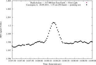
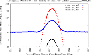
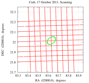
Figure 8: The radiometric response of the SRT for observations of Cass A at (a) 1.35 cm on September 28, 2011 and (b) at 6.2 cm on October 7, 2011, the latter against the background of the simultaneous responses in orthogonal polarizations at 18 cm. (c) Trajectory for scanning of the part of the sky containing the Crab Nebula on October 17, 2011, corresponding to the responses at 1.35 and 6.2 cm presented in Fig. 7b of the color insert. The contour shown at the center characterizes the angular size of the radio source.

5.6 Discussion of Results

In the absence of phase errors, the full width at half-maximum (FWHM) of the main lobe of the antenna beam $\vartheta_{0.5}$ and the aperture efficiency (AE) $\eta$, equal to the ratio of the effective to the geometrical area, depend on the distribution of the amplitude and phase of the electric field over the dish aperture and the level of illumination of the dish edge. For an ideal parabolic reflector with a circular aperture of diameter $D$, with some types of theoretical relations for the amplitude distribution of the co-phased field, the expected beam width $\vartheta_{0.5}$ and aperture efficiency $\eta_{0}$ at a wavelength $\lambda$ can be estimated in the co-phased case using the relations [50–52] $\vartheta_{0.5}=\alpha_{D}\cdot\lambda/D$, where $\alpha_{D}\approx 1.0{-}1.5$, and $\eta_{0}\approx 1.0{-}0.55$, depending on the law for the the field distribution. The lower the illumination of the dish edge, the lower the value of $\eta_{0}$ and the higher the value of $\alpha_{D}$; these values are close to unity only in the case of uniform field amplitudes all over the aperture. Phase distortions of the co-phased field in the aperture will additionally increase $\alpha_{D}$ and decrease $\eta_{0}$; i.e., increase the main lobe of the antenna beam and decrease the effective area.

Comparing these values of $\alpha_{D}$ with the values $\alpha_{D}\approx 1.2$ obtained from measurements of the SRT (see parameters 1.10 and 2.10 in Table 2) shows that the measured beamwidths at 92, 18, and 6.2 cm are close to the theoretically expected values. The most substantial differences between the inflight parameter measurements and the predicted or expected values obtained earlier in tests of the SRT in Pushchino [47] occurs for the effective area and the shape of the antenna-beam main lobe at 1.35 cm, and the SRT system noise temperature at 6.2 cm (Table 2). The use of any of the eight input bands is possible during operation in the bandwidth-synthesis regime at 1.35 cm. The presented results correspond to the central sub-band, $F_{0}$ (see Section 2.2.2).

5.6.1. 1.35 cm (central sub-band $\mathbf{F}_{\mathbf{0}}$). The measured FWHM level of the main lobe of the antenna beam corresponds to an ellipse with axes $\vartheta_{0.5}\times\varphi_{0.5}$ = $6.0^{\prime}\times 13^{\prime}$ with a relative error of $5\%$, compared to the expected circular beam with a diameter of $5.6^{\prime}\pm 10\%$. This is clearly visible in the source-scanning responses (Fig. 7b in the color insert and Fig. 8c). The measured effective area is 7.5 m² $\pm 13\%$, instead of the predicted value 27 m² $\pm 10\%$, or at least the projected value 23 m² $\pm 15\%$. These expected values for the beam and area were obtained during ground tests of the SRT in Pushchino in 2004. The difference between the effective area obtained in the ground tests and the effective area of an ideal parabolic surface ($40{-}45$ m²) can be explained in a natural way as an effect of the random uncertainty in the realization of the dish surface, which has an rms deviation no worse than the projected value $\sigma=0.77$ mm, as was specified via the tolerance $d=\pm 2$ mm ($|d|=2.6\sigma$ [43]). The reduction of the effective area to 7.5 m² could be explained in this same way, but with $\sigma\approx 1.4$ mm, or in some other usual way (e.g. a systematic quadratic phase error in the antenna aperture, with its maximum value ${\sim}1.5\pi$; see the Appendix), if it weren’t for the simultaneous observation of appreciable distortion of the main lobe of the antenna beam.

Such distortions of antenna beams in parabolic antennas are due mainly to three types of systematic phase distortions in the amplitude–phase distribution of the field over the dish aperture [50–53]: quadratic distortions, cubic (coma) distortions, and astigmatism of the dish and/or feed. Either the dish or feed could be responsible for quadratic and cubic distortions, or alternately, a shift of the feed from the dish focus in the directions along (for quadratic distortions) or transverse (for coma) to the paraboloid axis. Asigmatism occurs when the points of optimal focus in two main mutually orthogonal planes perpendicular to the aperture do not coincide [50]. This means that the optimal focus point for a feed mounted in the position with minimum aberration (and therefore with the minimum width for the main lobe of the antenna beam) is different in these two planes: each has its own focus point, and there is no single phase center. In this case, there usually exists some common “equivalent optimal-focus center” or “equivalent phase center” near the middle of these positions, where it is possible to minimize phase aberrations and distortion of the antenna beam [50, 53]. The phase errors in the aperture are the sum of these three types of errors associated with the dish, feed, and shift of the feed from the dish focus [54, 55]. Therefore, it is not possible to uniquely establish the real origin of phase distortions in the antenna aperture based purely purely on the results of inflight tests, without additional data or hypotheses.

A detailed analysis of this problem (see the Appendix) shows that the observed ellipticity of the main lobe of the antenna beam and the measured effective area at 1.35 cm can be explained most simply as the effects of a systematic quadratic error in the distribution of the phase along the $\varphi$ axis of the order of $1.5\pi$ on the antenna aperture and astigmatism due to the feed, in addition to the random error in the realization of the parabolic SRT dish surface with the projected rms deviation of $\sigma=0.77$ mm. Such a systematic phase error along one axis in the aperture could arise, for example, in the case of astigmatism of the feed with a quadratic phase error simultaneous with a shift of the optimal-focus center of the feed relative to the dish focus by about 0.3 cm along the paraboloid axis, with the distance between the two such centers of focus of the feed being $b\sim 2$ cm. Evidence supporting this hypothesis is presented by estimates obtained using one of the phase-distortion models in the Appendix, obtained using the results of numerical computations of the amplitude–phase beam of the antenna-feed assembly [56]. The computations of [56] suggest possible astigmatism and quadratic aberrations of the dish illumination with values close to those required to explain the results of the 1.35-cm measurements.

Attempts to derive a self-consistent explanation for all the antenna measurements without including astigmatism of the feed were not successful (see the Appendix). However, this is only one possible explanation. Formally, it is also possible that the observed systematic phase errors in the aperture are due to the antenna dish rather than the feed. However, there is currently no firm basis for this, or sufficient data for a quantitative analysis to justify such a conclusion. The simple explanation for the asymmetry of the antenna beam as corresponding to a strong asymmetrical deformation of the dish, such that the size of the aperture is a factor of two smaller in one plane (to 5 m), should affect the results at other wavelengths as well. This is in contradiction with the “good” results for the antenna measurements at 6.2, 18, and 92 cm, which are close to their predicted values.

5.6.2. 6.2, 18, and 92 cm. In contrast to the other wavelengths, all measurements at 6.2 cm were conducted separately in the polarization channels. Turning on both simultaneously led to extremely high output signals that could not be reduced with attenuators. A distortion of the autospectra of the output videoband for the channel with right-circular polarization was also observed in the interferometric regime. These facts suggest a degrading of the matching between the AFA polarization channels and free space and/or with the LNA in part of the 6.2-cm AFA input–LNA input antenna-feeder track, which worsened the isolation between the polarization channels. This led to an increase in both reactive and active losses in this section when the channels are turned on separately, causing an increase in the system noise temperature in accordance with (5.7), and also to self-excitation of the LNA when both channels are turned on. Analysis of this situation is ongoing.

In all the antenna measurements, the preliminary noise-generator antenna temperatures $T_{\mathrm{NS}}$ obtained from pre-flight ground measurements were used, with “recalculation” of $T_{\mathrm{NS}}$ to the SRT input using formula (5.7c) together with the measured or calculated [25] losses in the antenna-feeder tract. It was planned to correct these values using the results of inflight tests. This correction was not applied for 92, 18, and 1.35 cm, however, the $T_{\mathrm{NS}}$ correction was applied for 6.2 cm: 1) assuming a corresponding increase in the losses in the AFA [i.e., a decrease in $K_{2}$ in (5.7b) and (5.7c)] and 2) neglecting distortions from the antenna beam that decrease the effective area, consistent with the calculations of [56] and estimates of parameters 4.2 and 5.2 for 6.2 cm in Table 3. This correction led to a corresponding increase in the effective area $A_{\mathrm{eff}}$ and system noise temperature $T_{\mathrm{sys}}$ at 6.2 cm (i.e., to an “improvement” in $A_{\mathrm{eff}}$ and a “worsening” of $T_{\mathrm{sys}}$).

This correction made it possible to obtain a general, self-consistent explanation for the measured wavelength dependences of the effective area of the SRT at all wavelengths using a single approach to taking into account phase errors. It can also simultaneously explain the corresponding increase in the system noise temperature at 6.2 cm, and possibly partially at 92 cm, according to (5.7), as being due to an increase in the losses $L_{2}$ in the AFA compared to the predicted values. The contribution from the sky background is also appreciable for the 92-cm SRT noise temperature, and can vary significantly with direction; this can fully or partially explain the 20% increase in the measured noise temperature $T_{\mathrm{sys}}=200$ K above the expected value. Based on estimates using published distributions of the sky brightness temperature and relations (5.7) and (5.7a), the minimum contribution of the sky background when the antenna is pointed toward the Galactic pole should be about 60 K, which is included in the expected temperature $T_{\mathrm{sys}}^{\mathrm{(opt)}}=164$ K [25].

We emphasize that the AFA losses $L_{2}=1/K_{2}$ appear in three terms in (5.7), which is not always taken into account when obtaining rough estimates. Note also that, in contrast to calibration using the antenna temperature, which is necessary for antenna measurements, the astronomical-calibration method usually used for both the ground radio telescopes and the SRT does not depend on these characteristics and corrections, since the calibration factors are proportional to $T_{\mathrm{sys}}/A_{\mathrm{eff}}$ (for the SEFD $F_{\mathrm{sys}}$) or $T_{\mathrm{NS}}/A_{\mathrm{eff}}$ (for $F_{\mathrm{NS}}$). Therefore, this calibration can be carried out for observations of astronomical sources without knowledge of the absolute values of the temperatures $T_{\mathrm{NS}}$ and $T_{\mathrm{sys}}$ (see Section 5.1 and [45]).

5.6.3. Pointing and Scanning corrections. These corrections were measured by scanning areas containing sources along the $\vartheta$ and $\varphi$ axes (see the example in Fig. 7b in the color insert and in Fig. 8c). The results of such scanning were used to find the central cross section of a source, for which the scanning process was repeated a number of times in the forward and reverse directions along each axis. The forward and reverse scans were averaged separately using the telemetry data for the standard coordinate information, and the difference in the calculated and measured coordinates for the positions of the signal maxima were calculated, yielding the desired corrections to the calculated coordinates.

The measurements of the coordinate errors along the $\vartheta$ axis (with the smaller antenna beam, $\vartheta_{0.5}=6^{\prime}$, were systematically different for the “forward” and “reverse” scans, and the scanning curve had the “two-humped” form characteristic for ground telescopes, with values of $(3.7^{\prime}\pm 0.2^{\prime})$ for one maximum and $1.3^{\prime}\pm 0.2^{\prime}$ for the other. These data were used to introduce a constant pointing correction $\Delta\vartheta_{p}=2.5^{\prime}$, equal to the mean of these values, which was subsequently applied. The two-humped appearance of the scans in opposite directions remained with roughly the previous delay, corresponding to $|\Delta\vartheta_{s}|=1.2^{\prime}\pm 0.2^{\prime}$ relative to the calculated value, still with a time delay that was independent of the forward or reverse direction of the scanning, but now relative to the zero mean value between the maxima. We interpret this delay in the electrical axis for motion of the SRT relative to the new calculated position of the axis as a systematic scanning error (Table 2). No such correction was introduced for the other axis, since the results in that case were within the uncertainties.

Roughly half the measured time interval between the humps can be explained by a delay in the response when the signal is integrated at the radiometer output (see the discussion of this effect in [57]). The main origin of this type of two-humped curve for ground telescopes (which is absent for the SRT) is believed to be backlash in the control mechanisms. The origin of the analogous behavior of the SRT could be related to similar delays during integration of the signals in the electronic system of the star sensors and the spacecraft-motion control chains, or some other effect, and requires further study. The hypothesis of elastic deformations of the boom on which the SRT focal container is fixed contradicts the telemetry results, which indicate a fairly uniform speed in sections of the motion.

5.6.4. Telemetry Noise. Analysis of the telemetry data showed the presence of additional “telemetry noise” for the digital radiometric outputs in both channels of the 18 and 92-cm receivers. This has the form of a background consisting of “packets” of short impulsive spikes, and is characteristic of errors in recording individual bits: the amplitude of their “variability” is not random, and repeats systematically, varying in a step-like fashion “from packet to packet”. Comparison with the telemetrized parameters of “ADC-ready” receivers suggests that this noise is due to the fact that the standard telemetry system does not take the ready signal of the analog-to-digital converters (ADCs) in the receivers into account when interrogating all the sensors with fixed velocities. As a result, the interrogation of the digital sensors sometimes occurs before the ADCs in these instruments are in the ready state. Such noise was first discovered during the acceptance tests. A simple and effective means of filtration was found and applied, which made it possible to eliminate this problem for the inflight SRT antenna measurements. No such noise is present in the analog outputs of the 18 and 92-cm receivers or in all outputs of the 1.35 and 6.2-cm receivers.

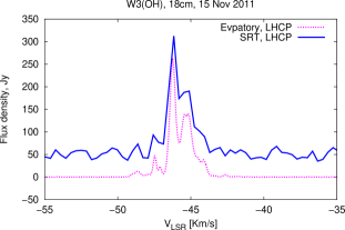
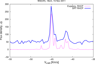
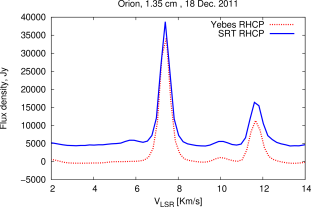
Figure 9: Simultaneous two-antenna observations of cosmic maser sources. (a, b) 18-cm observations of W3(OH) by the SRT on October 30, 2011 in (a) left- and (b) right-circular polarization. (c) 1.35-cm observations of the Orion KL star-forming region by the SRT and the 32-m Zelenchuk radio telescope of the Institute of Applied Astronomy on December 18, 2011. The SRT spectra are shifted in amplitude for clarity.

5.7 Independent Verification of the Interferometric Regime Using Radio Lines

It is possible to use observations of several strong cosmic OH (18 cm) and water (1.35 cm) maser sources to test the operation of the receiver equipment, HDRRC radio line, and correlator in the interferometric regime in K and L bands. Several measurement sessions were carried out for this purpose, in which such objects were observed simultaneously in right- and left-circular polarizations with the SRT and several ground telescopes. The star-forming region Orion KL and W3(OH) were chosen for the 1.35-cm observations, and W3(OH) for the 18-cm observations. The high fluxes of these objects and the presence of strongly polarized components in their spectra enabled a comparative analysis of the characteristics of the receiver–recorder equipment and its suitability for such observations.

5.7.1. Observations. 1. W3 (OH). The star-forming region W3(OH) is located at a distance of about 2 kpc [58] in the Perseus arm of the Galaxy, and is among the most studied objects of this type. Strong maser emission in both OH lines and water lines (with the latter approximately $6^{\prime\prime}$ to the East of the OH masers) is observed toward W3(OH). The spectrum contains polarized features, enabling estimation of the polarization properties of the SRT by comparing spectral profiles obtained simultaneously with the SRT and a well-understood ground instrument.

2. Orion KL. This well known star-forming region is located at a distance of $437\pm 19$ pc [59] in the constellation Orion. The water masers undergoes flares, as a result of which individual spectral features can reach flux densities of several million Jy [60]. Since the beginning of 2011, Orion KL has been in a phase of enhanced activity [61], and its flux at the epoch of our observations was approximately $3.5\times 10^{4}$ Jy, making this maser the strongest object in its class in the sky. The object is especially convenient for observations, since its high flux density makes it possible to achieve high signal-to-noise ratios in modest integration times, even with the low sensitivity of the SRT in K band.

The observations of W3(OH) were carried out in October and December 2011, and the observations of Orion KL in December 2011, as part of the program of inflight receiver tests and fringe searches. Below, we analyze the spectra of these objects obtained with the SRT in an autocorrelation regime (using data that have passed through the HDRRC channel) and at ground radio telescopes participating in simultaneous observations.

5.7.2. Analysis of the Spectra. Figures 9a, 9b, and 9c show that the maser-line profiles obtained on the SRT at 1.35 cm for Orion KL at the frequency of the 22235.08-MHz water line and at 18 cm for W3(OH) at the frequency of the 1665.4018 MHz OH line correspond nearly fully to the line profiles obtained on large ground telescopes. The small observed differences in the spectrum profiles measured by the ground telescopes and the SRT are most likely due to the low signal-to-noise ratio of the SRT data. Figures 9a and 9b for W3(OH) show that, due to the appreciable difference in the appearance of the spectral features in the different polarizations, it is easy to identify the received polarization (left- or right-circular polarization; compare with Fig. 2 of [62]). Such sources can also serve as an additional tool for monitoring the pointing and verifying the correctness of the frequency tuning of the equipment at 1.35 and 18 cm. Another task that can be addressed with such studies is estimation of the sensitivity of the SRT based on spectral observations in the L and K bands. The parameters of the ground telescope that is used can be used to estimate the flux from a source at the observing epoch, and thereby the SRT sensitivity. Such estimates were obtained based on observations of W3(OH) in the K and L bands and of Orion KL in the K band. The resulting SEFDs are 3400 Jy for the L band and about 36 000 Jy for the K band.

5.8 Conclusions

1. The derived equivalent system noise temperature of the SRT coincides with theoretical estimates at 92, 18, and 1.35 cm within $20\%$, but exceeds the calculated value at 6.2 cm by a factor of two, which lowers the interferometer sensitivity of this last band by a factor of $\sqrt{2}$ (for a fixed integration time). The origin of this enhanced noise temperature is probably an increase in losses in the antenna-feeder tract (most likely in the section running from the AFA to the LNA), compared to the losses calculated based on laboratory measurements carried out on the Earth.

2. The FWHM of the main lobe of the SRT beam agrees with theoretical expectations and measurements obtained in ground tests within the errors at 92, 18, and 6.2 cm, but differs appreciably from the expected value at 1.35 cm: the transverse cross section of the main lobe at the half-maximum level is close to elliptical, with axes $\vartheta_{0.5}\approx 6.0^{\prime}\pm 5\%$ and $\varphi_{0.5}\approx 13^{\prime}\pm 5\%$, rather than the expected circular cross section with diameter $5.5^{\prime}\pm 10\%$. The profile of the longitudinal cross section of the main lobe in the plane in which it is wider is appreciably asymmetrical.

3. The effective areas of the SRT in flight are close to the calculated values and the values measured in ground tests at 92, 18, and 6.2 cm. The effective area at 1.35 cm is a factor of 3.6 smaller than the value obtained in ground tests, 27 m² $\pm 10\%$, and a factor of three smaller than the projected area, 23 m² $\pm 15\%$, which reduces the sensitivity in the interferometric regime by nearly a factor of two (for a fixed integration time).

4. Estimates based on calculated values of the amplitude–phase beam of the AFA in a simple model for the phase errors in the antenna-feeder system lead to the following conclusions about the SRT in flight.

– The mean dish surface profile may be close to parabolic, with its rms deviation equal to the predicted value, 0.77 mm.

– The antenna feed may have: a) quadratic phase errors with the maximum error in the feed phase at the edge of the disk equal to roughly ${-}100^{\circ}$ at 1.35 cm and ${-}35^{\circ}$ at 6.2 and 18 cm (according to the calculated phase beams for these feeds); b) astigmatic aberrations at 1.35 cm, approximated by the presence of two equivalent centers of focus of the feed — centers 1 and 2 in orthogonal planes 1 and 2, respectively — shifted from the dish focus by approximately 7 mm toward the dish in plane 1 and 13 mm away from the dish in plane 2; c) a common center of optimal focus of the feed (between centers 1 and 2), which is shifted from the focus of the unfurled antenna by approximately 3 mm from the dish along the longitudinal axis of the antenna.

– These phase errors in the illumination of the dish surface may provide the main reason for the measured decrease in effective area and the ellipticity of the main lobe of the SRT antenna beam at 1.35 cm compared to expected values.

5. The results of radio adjustments show that the mean pointing error along the axis with the smaller beam width is $3.7^{\prime}\pm 0.2^{\prime}$ for scanning of a source in one direction and $1.3^{\prime}\pm 0.2^{\prime}$ for scanning in the reverse direction. This can partially be explained by a delay of the response due to integration of the signal in the radiometer output, and requires further study. Based on these measurements, a constant pointing correction was introduced, $\Delta\vartheta_{p}=2.5^{\prime}$. The remaining scanning error, $|\Delta\vartheta_{s}|=1.2^{\prime}\pm 0.2^{\prime}$, characterizes a delay in the signal maximum relative to its calculated position during scanning in either direction, and is due to a systematic error in the antenna motion. The pointing error along the axis with the larger antenna beam lies within the measurement uncertainties, and does not exceed $1.5^{\prime}$; this error was not corrected for in subsequent observations.

6. Comparison of the autocorrelation spectra for two strong maser sources in L and K bands indicates that the spectral observational regime of the SRT is functioning normally. Such observations can be used to monitor the frequency tuning and polarization regime during observations. Estimates of the SRT sensitivity based on observations of radio lines are in agreement with the results of continuum observations. The full determination of the polarization parameters of the radio telescope, which is possible using specially planned observations of several bright maser sources such as Orion KL, remains incomplete.

6 VERIFICATION OF THE FUNCTIONING OF THE GROUND–SPACE INTERFEROMETER (FIRST FRINGES) AND FIRST OBSERVATIONAL RESULTS

In this section, we present a brief survey of the first results obtained in the interferometric regime. These results will be discussed in more detail in future articles by various international groups involved with the fringe searches and the Early Science Program, after a more thorough analysis of the data.

The detection of the interferometer signal between the RadioAstron SRT and ground radio telescopes has demonstrated the overall successful operation of the space–ground VLBI system at all four wavelengths: 92, 18, 6.2, and 1.35 cm (Figs. 7c–7g in the color insert). The first signal from the space interferometer was obtained for observations made on November 15, 2011, of the quasar 0212+735 at 18 cm, when the spacecraft was about 100 000 km from the Earth and the projected baseline between RadioAstron and the 100-m Effelsberg telescope was $B=8100$ km (Fig. 7c in the color insert). In all, 20 test sessions of the interferometer have been conducted thus far. Interferometric observations of the pulsar PSR 0950+08 at 92 cm were carried out with the spacecraft at the record distance of 300 000 km (a projected baseline of about 220 000 km) on January 25, 2012, with the participation of the largest ground radio telescope — Arecibo, with a diameter of 300 m (Figs. 7f, 7g in the color insert). Most interferometric observations have used the onboard hydrogen maser, but successful test sessions have also been carried out in a regime where a coherent signal from the hydrogen maser at the tracking station in Pushchino is sent to the spacecraft and then sent back to the tracking station (a so-called closed phase loop regime).

In the interferometric regime, the sensitivity of the system of two telescopes is proportional to the square root of the product of the effective areas of these telescope; thus, the combination of the 10-m SRT and a 100-m ground radio telescope has a sensitivity equivalent to a pair of two 30-m telescopes. It is not possible to obtain the results of a ground–space interferometer measurement immediately after the measurement itself. The scientific data recorded at the various radio telescopes are first transmitted to a reduction center for correlation (detection of the interferometer response). This correlation can be carried out only after high-precision reconstruction of the spacecraft orbit at the ballistic center.

Figure 10: Simultaneous three-antenna observations of the giant pulses of the Crab Nebula pulsar on November 14, 2011, carried out by the SRT, the Badary 32-m telescope (near Irkutsk, Russia), and the 70-m Evpatoria telescope (Ukraine) at 18 cm.

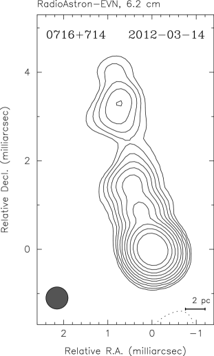
Figure 11: 6.2-cm image of the rapidly variable BL Lac object 0716+714. The observations were carried out using the SRT and the EVN on March 14-15, 2012 as part of the RadioAstron Early Science Program on AGNs. This image was constructed using an antenna beam with a FWHM of 0.5 mas, whose cross section is shown in the lower left-hand corner of the figure. The lowest contour is 0.25 mJy/beam, and the contours increase in steps of a factor of two. The peak intensity is 0.43 Jy/beam. The “beam” is the solid angle of the shown cross section.

The reduction and analysis of data obtained using the RadioAstron ground–space interferometer are carried out at the ASC in collaboration with other participants of the project. First and foremost, this includes the correlation of the data flows recorded at the individual radio telescopes at rates of 128 or 256 Mbits/s, including the space segment of the SRT (128 Mbits/s), using the RDR-1 recording system created at the ASC [63] and the Mark5 recording system developed in the USA [64]. The FX correlator of the ASC is based on a computing cluster with a performance of 1 Tflop/s and a RAID data-storage system with a volume of up to 200 Tbyte. The technical characteristics of the processor cluster of the ASC SDRC is able to handle data flows from 10 stations including the SRT with integrated data rates of up to 2.56 Gbits/s; accordingly, it can process up to 45 interferometer baselines. This can be done essentially at the rate at which the data were recorded in real time.

The detection of an interferometer response is not in itself a final scientific result. However, with certain assumptions about the structure of a compact feature, it can be used to estimate its angular size and brightness temperature. Multiple observations with various telescope configurations, most importantly with various positions of the spacecraft in its orbit, are necessary to derive trustworthy conclusions about the structure of a studied object. The required set of such configurations can be realized in observations over no less than one calendar year. The planned observing strategy is to study a sample of radio sources over the course of a year (and sometimes several years), after which a multi-faceted analysis is applied to draw basic conclusions about the structure and physical conditions in the studied objects.

The RadioAstron Early Science Program has been underway since February 2012, and is overseen at the ASC and carried out by international groups of researchers formed in the framework of the project. Thus far, the interferometer responses from the pulsars PSR 0950+08, PSR 0531+21 (Crab), PSR 0833-45 (Vela), and PSR 1919+21, the AGNs 0212+735, 0716+714, 0748+126, 0754+100, 2013+370, 0851+202 (OJ287), 1954+513, and 2200+420 (BL Lac), and the Galactic maser W51 have been measured (see the RadioAstron newsletters for 2011–2012 [65]). These responses were obtained for projected baselines for the ground–space interferometer of less than 10 000 km to about 250 000 km, roughly 20 Earth diameters.

After confirmation of the possibility of observing giant pulses from the Crab Nebula pulsar (at a distance of 1 kpc) with the SRT, correlations between the 18-cm pulses recorded at the SRT and the Evpatoria, Svetloe, Zelenchuk, and Badary ground radio telescopes were detected for observations made on November 14, 2011, for projected baselines of up to $B=40\,000$ km (Fig. 10). This testifies that scattering of the image in the interstellar medium along the path from the pulsar to the observer at 18 cm was no greater than the angular resolution of the interferometer, 400 $\mu$as.

Interferometer observations of ordinary pulses of the nearby pulsar PSR 0950+08 (260 pc; Fig. 7f in the color insert) did not detect interstellar scattering even at 92 cm with projected baselines of up to $B=220\,000$ km. In this way, an angular resolution of 370 $\mu$as was achieved at meter wavelengths. Observations of this pulsar over one hour (Fig. 7g in the color insert) enabled the detection of variability of the visibility function with such long baselines, opening possibilities for studying the parameters of turbulence of the interstellar plasma and the achievement of even higher angular resolution using the “interstellar interferometer” principle [66]. Scattering in the interstellar medium was detected for another nearby pulsar Vela, at a distance of ${\sim}300$ pc. This pulsar was observed at 18 cm jointly by the SRT and the largest radio telescopes of the Southern hemisphere in May 2012. The Parkes, Mopra, Hobart (all Australia), Hartebeesthoek (South Africa), and Tidbinbilla (Australia) radio telescopes participated in these observations. The reduction of these data showed that the structure of the interferometer response changes completely at a projected baseline of 100 000 km (numerous narrow brightenings are observed), indicating that we are observing the results of a multi-path propagation of the radio waves through inhomogeneous interstellar plasma.

An example of the interferometer response to an H₂O maser source (1.35 cm) in the star-forming region W51 obtained during observations with the SRT and the 100-m Effelsberg radio telescope is presented in Fig. 7e (color insert). These observations were carried out on May 12, 2012, with a projected ground–space baseline of 14 500 km (1.14 Earth diameters), yielding an angular resolution of 80 $\mu$as.

The largest number of interferometric observations have been associated with studies of the structure of AGNs. Interferometry responses at 6.2 cm with projected values for the SRT–Effelsberg baseline $B=92\,000$ km, or 7.2 Earth diameters, have been obtained for the two quasars OJ 287 (which some authors have suggested may harbor a binary supermassive black hole; see, for example, [67]) and BL Lacertae (the prototype of the class of BL Lac objects). This yields brightness temperature estimates for the dominant feature in the compact jet — the core — of about $10^{13}$ K or somewhat higher. This exceeds the well known inverse-Compton limit for the brightness temperature [68], but the emission can still be explained in the standard model with incoherent synchrotron emission from a Doppler-boosted relativistic jet [69].

For the AGN 0716+714, which is among the most rapidly variable extragalactic objects, interference fringes were detected at 6.2 cm at multiple projected ground–space baselines from roughly 1.5 to more than 5 Earth diameters. The international group working on the Early Science Program constructed an image of this object (Fig. 11) and estimated the parameters of the core. The width at the base of the jet in the core region is approximately 70 $\mu$as, or 0.3 pc, and the brightness temperature is $2\times 10^{12}$ K. Note that these parameters were measured at an epoch of minimum activity of this object.

7 CONCLUSION

The RadioAstron space radio telecope has been inserted into the nominal orbit, and successfully tested in both autonomous and ground–space interferometric regimes at all four operational wavelengths (1.35, 6.2, 18, and 92 cm). The main parameters of the SRT and interferometer have been determined. Record angular resolutions, more than a factor of 10 better than is attainable on Earth, have been achieved. The sensitivity derived from inflight tests is sufficient to enable a full-scale program of scientific studies. Further measurements will be used to refine the limits of possible observations in several directions: 1) determination of the flux limit for the detection of linearly polarized emission, 2) use of evolutionary changes in the orbit to obtain fuller information about the structure of objects (in paraticular, to attain ultra-high angular resolution both along and across jet structures in AGNs), 3) application of multi-frequency synthesis in image construction, 4) analysis of Faraday rotation of the plane of polarization based on multi-frequency observations, 5) study of variability of the source structures, 6) high-precision astrometric measurements, 7) analysis of possibilities for high-precision determination of the spacecraft motion, etc.

Brief reports about current results are regularly issued in RadioAstron newsletters [65].

POSSIBLE INTERPRETATION OF THE 1.35-CM ANTENNA MEASUREMENTS

The measured ellipticity of the main lobe of the SRT antenna beam at the half-maximum power level could be due to comparatively large phase errors along the $\varphi$ axis combined with relatively modest distortions in the orthogonal $\vartheta$ axis. We will refer to the orthogonal azimuthal planes corresponding to longitudinal cross sections of the main lobe of the SRT beam with widths $\vartheta_{0.5}$ and $\varphi_{0.5}$ along these axis as “plane 1” and “plane 2”, and to the corresponding phase errors over the dish aperture as $\delta\varphi_{1}$ and $\delta\varphi_{2}$. The main lobe of the antenna beam in plane 2 (along the $\varphi$ axis) turned out to be a factor of 2.2 wider than in plane 1, appreciably asymmetric, and somewhat shifted relative to the calculated geometrical axis of the SRT; these properties are characteristic for distortions that arise due to combinations of all three types of aberration — quadratic, cubic, and astigmatic.

Physically, the maximum quadratic and cubic phase errors in ground radio telescopes usually indicate defocusing of radiation reflected from the edge of the dish that arises due to transverse or longitudinal shifts of the feed from the focus; such errors are characteristic even for ideal paraboloids with modest ratios of the focal distance $F$ to the diameter of the dish aperture $D$ ($F/D\approx 0.43$ for the SRT). In this case, assuming that the feed was mounted at the calculated geometrical focus of the paraboloid with the projected accuracy (${\pm}1$ mm), such errors could appear, for example, if the real focus of the unfurled dish did not precisely coincide with the calculated position. However, other origins are also possible, including peculiarities of the illumination of the dish (see below).

Rough quantitative estimates yield for the phase error in plane 1 at the dish edge (relative to the aperture center) $\delta\varphi_{1}\approx 0$ (since $\vartheta_{0.5}$ is close to the predicted value for the undistorted beam within the errors, see parameters 1.10 and 2.10 in Table 2), while the error in plane 2 is $\delta\varphi_{2}\sim(2\pi/\lambda)R_{0}(\varphi_{0.5}-\vartheta_{0.5})=1.5\pi$, where $\lambda=1.35$ cm is the wavelength, $R_{0}=500$ cm the radius of the SRT dish, $\varphi_{0.5}=13^{\prime}$, and $\vartheta_{0.5}=6^{\prime}$.

The difference in the effective area can be explained quantitatively by the combination of a systematic error in the dish aperture $\varphi_{q}=\delta\varphi_{1}+\delta\varphi_{2}\sim 1.5\pi$ and random errors with the projected rms $\sigma=0.77$ mm, using the following formulas for the coefficients $\eta_{\sigma}$ and $\eta_{\varphi}$ for the decrease in the effective area of the antenna aperture [43, 55]:

$$\eta_{\sigma}=\exp[{-}(4\pi\sigma/\lambda)^{2}],$$

$$\eta_{\varphi}=6.55(1.01-0.2\cos\varphi_{q})/(5.3+\varphi_{q}^{2}).$$

Whence, $\eta_{\sigma}=0.60$, $\eta_{\varphi}=0.24$, $\eta=\eta_{\sigma}\eta_{\varphi}=0.15$, and we obtain for the effective area $A_{0}$ “corrected” for these losses $A_{0}=A_{\mathrm{eff}}/\eta_{\varphi}=31$ m² and $A_{0}=A_{\mathrm{eff}}/\eta=50$ m² for $A_{\mathrm{eff}}=7.5$ m². These values of $A_{0}$ confirm that the two types of errors considered could, in principle, be the main causes of the reduction in $A_{\mathrm{eff}}$ and the aperture efficiency (reductions of AE from $1$ to $0.5{-}0.6$ are typical for single-dish antennas, and are usually determined by other well known factors, most importantly over-illumination of the dish and incidence of radiation toward the dish edge (depending on the feed beam) and errors in the dish surface; see, for example, Appendix 5 in [43]). Note that, since formula (A.2) was obtained assuming a Gaussian amplitude distribution over the aperture, with illumination of the aperture edge to the 0.1 level [55], we expect that this formula is more applicable for our estimates, in spite of the fact that this takes into account only quadratic, not cubic, phase errors. We will neglect area losses due to cubic phase errors (or coma-type aberration) here.

The reduction of the effective area can also formally be explained using only $\eta_{\sigma}$ with an rms deviation $\sigma\approx 1.4$ mm. This value of $\sigma$ would then be considered some kind of “effective” random error. In our case, it is possible to distinguish the similar contributions of $\sigma$ and $\varphi_{q}$ only because of the observed ellipticity of the antenna beam.

The observed scatter in the measured effective areas about the mean area (more than $10\%$) could indicate variability of the random and systematic errors ($\sigma$ and $\varphi_{q}$) due to variation in the temperature distribution over the dish surface with variation in the SRT orientation relative to the Sun. For example, it follows from (A.1) that, with $\sigma\approx 0.77$ mm, varying $\sigma$ by even 0.1 mm could lead to appreciable variations in the effective area of the SRT at 1.35 cm. This strong dependence on the random error is due to the closeness of the central wavelength at 1.35 cm to the so-called “limiting” wavelength of the radio telescope $\lambda_{\mathrm{min}}$, which is equal to $\lambda_{\mathrm{min}}\approx(20{-}16)\sigma$ (according to the practical criterion for estimating this limiting wavelength given in [43]), and depends on the accuracy of the realization of the dish surface, usually relative to an ideal parabolic surface. We have for the SRT $\lambda/\sigma=18$ for $\lambda=13.5$ mm and the projected rms deviation $\sigma=0.77$ mm.

Table 3: Modeling of phase errors in the antenna system: three models for the contribution of feed phase errors [56] to the decrease in $A_{\mathrm{eff}}$ and the aperture efficiency AE, as well as the ellipticity of the cross section of the main lobe of the SRT beam

Parameter	K (1.35 cm)	C (6.2 cm)	L (18 cm)	P (92 cm)
SRT in flight, 2011–2012:
1.    $A_{\mathrm{eff}}$, m2	7.5	35	41	30
2.    AE = $A_{\mathrm{eff}}/A_{\mathrm{geom}}$	0.1	0.45	0.52	0.38
3.    $\eta_{\sigma}=\eta_{\sigma}(\sigma=0.77$ mm)	0.60	0.98	1.00	1.00
4.    Model 1: $\varphi_{q}=2\delta\Psi_{\mathrm{max}}$.
4.0   $\delta\Psi_{\mathrm{max}}$ (in degrees of phase)	-100	-35	-35	–
4.1   $\varphi_{q}$ (in degrees of phase)	-200	-70	-70	–
4.2   $\eta_{\varphi}=\eta_{\varphi}(\varphi_{q})$	0.45	0.91	0.91	–
4.3   $\eta=\eta_{\sigma}\eta_{\varphi}$	0.27	0.89	0.91	–
4.4   $A_{0}=A_{\mathrm{eff}}/\eta$, m2	28	39	45	–
4.5   AE${}_{0}=A_{0}/A_{\mathrm{geom}}$	0.35	0.50	0.57	–
5.    Model 2: $\varphi_{q}=2\delta\Psi_{\mathrm{max}}+\delta\varphi_{x}$.
$\delta_{1}=5.3$ mm
5.0   $\delta\varphi_{x}=k\delta_{1}/2$ (in degrees of phase)	-70	-15	-5	–
5.1   $\varphi_{q}$ (in degrees of phase)	-270	-85	-75	–
5.2   $\eta_{\varphi}=\eta_{\varphi}(\varphi_{q})$	0.24	0.87	0.89	–
5.3   $\eta=\eta_{\sigma}\eta_{\varphi}$	0.15	0.85	0.89	–
5.4   $A_{0}=A_{\mathrm{eff}}/\eta$, m2	50	41	46	–
5.5   AE${}_{0}=A_{0}/A_{\mathrm{geom}}$	0.64	0.52	0.59	–
6.    Model 3: $\varphi_{q}=\delta\varphi_{1}+\delta\varphi_{2}$;
$\delta\varphi_{1}=\delta\Psi_{\mathrm{max}}+k\delta_{11}/2=0$;
$\delta\varphi_{2}=\delta\Psi_{\mathrm{max}}-k\delta_{12}/2=-1.5\pi$;
6.0   $\delta\varphi_{x}=k(\delta_{11}-\delta_{12})/2$ (in degrees of phase)	-70	–	–	–
6.1   $\varphi_{q}$ (in degrees of phase)	-270	–	–	–
6.2   $\eta_{\varphi}=\eta_{\varphi}(\varphi_{q})$	0.24	–	–	–
6.3   $\eta=\eta_{\sigma}\eta_{\varphi}$	0.15	–	–	–
6.4   $A_{0}=A_{\mathrm{eff}}/\eta$, m2	50	–	–	–
6.5   AE${}_{0}=A_{0}/A_{\mathrm{geom}}$	0.64	–	–	–
6.6   $\delta_{11}$, mm	7.5	–	–	–
6.7   $\delta_{12}$, mm	13	–	–	–

We emphasize that it is not possible to unambiguously establish the physical origins of phase distortions in the antenna aperture and distinguish the contributions to the errors of the dish, feed, and geometry of the antenna-feeder system based on the results of inflight tests of the SRT alone, without additional data or assumptions. We can only be sure that these are due to some total phase error over the aperture due to 1) differences between the real antenna reflecting surface and an ideal parabolic surface, 2) longitudinal and transverse shifts of the feed from the dish focus, and 3) peculiarities of the amplitude–phase beam of the feed (including, for example, different widths of the real amplitude beam of the feed in orthogonal planes, with the effective width of the illumination of the ideal dish being equal to the projected value in one plane, but a factor of two worse in the other plane, or astigmatism of the feed, when the dish focus and feed center of focus are close to each other in one plane but in appreciably different positions in the other plane).

The phase distribution of the field $\varphi(x)$ at a point $0\leq x\leq R_{0}$ in a dish aperture with radius $R_{0}$ can be written [54] $\varphi(x)=\Phi(x)-\Phi_{0}$, where $\Phi(x)$ and $\Phi_{0}$ are the initial field phases at the point $x$ and at the center of the aperture. $\Phi(x)=\Psi(\psi)+k(\rho+t)$ and is determined by the phase of the feed beam $\Psi(\psi)$ ($0\leq\psi\leq\psi_{0}$; here, $\psi$ is the angle from the dish focus between the points $x=0$ and $x\leq R_{0}$ ) and the lengths of the path $\rho$ from the feed to the dish and the path $t$ from the dish to the aperture ($k$ is the wavenumber). Therefore, $\Phi(x)$ is a function of the phase beam of the feed, the dish profile (with the deviation $\delta_{3}$ of the surface from an ideal surface), and the shift of the feed phase center relative to the paraboloid focus (by $\delta_{1}$ in the longitudinal and $\delta_{2}$ in the transverse direction relative to the antenna axis). The deviations of these factors from their projected values give rise to a total deviation of the phase distribution at the dish aperture from the projected (in the ideal case, close to co-phased) value $\delta\varphi(x)$, and can be estimated with sufficient accuracy for our purposes as [54]

$$\delta\varphi(x)=2\delta\Psi(\psi)+k[\pm\delta_{1}(1-\cos\psi)\\ -\delta_{2}\sin\psi-2\delta_{3}(1+\cos(\psi/2)].\mathrm{~{}~{}~{}~{}A.3}$$

Here, in the general case, $\delta\Psi(\psi)$ contains random and systematic deviations of the feed phase beam. The term with $\delta_{3}$ is associated with inaccuracy of the dish surface, the terms with $\delta_{1}$ and $\delta_{2}$ reflect a systematic “incursion” of the phase from the center of the aperture toward the edge due to the lack of coincidence between the dish focus and the feed centerof focus (with even and odd functions relative to the center of the aperture, respectively), and $k=2\pi/\lambda$ is the wavenumber. A plus sign in front of $\delta_{1}$ in (A.3) corresponds to a shift $\delta_{1}$ of the feed phase center from the focus toward the dish, while a minus sign corresponds to a shift from the dish.

The maximum phase incursion is reached at the edge of the aperture, with $\psi=\psi_{0}=60^{\circ}$ for the SRT. Thus, we can neglect terms with $\delta\Psi(\psi)$ and $\delta_{3}$ in (A.3). Assuming $k|\delta_{2}|\sin\psi_{0}=\varphi_{q}\sim 1.5\pi$, we obtain the rough estimate for the transverse shift $|\delta_{2}|\sim 12$ mm. Analogously, assuming $k|\delta_{1}|(1-\cos\psi_{0})=\varphi_{q}$ yields the estimate of the longitudinal shift $|\delta_{1}|\sim 20$ mm, and the estimate for the maximum distance between the feed phase center and dish focus $\delta_{\mathrm{max}}=(\delta_{1}^{2}+\delta_{2}^{2})^{1/2}\sim 23$ mm. On the other hand, if the main contribution in (A.3) is made by phase distortions of the feed beam, setting $2\delta\Psi(\psi_{0})=\varphi_{q}\sim 1.5\pi$ yields the estimate for the maximum feed phase error at the edge of the dish required for this $\delta\Psi(\psi=60^{\circ})\sim 0.75\pi=135^{\circ}$.

Let us estimate the phase errors in the antenna-feeder system in a simple model (Table 3), based on the computational data [56] for the amplitude–phase beams of the SRT feeds and the projected rms deviation for the dish surface compared to an ideal parabolic surface $\sigma=0.77$ mm. Let us consider three types of model:

1) the AFA is at the focus,

2) the AFA is not at the focus,

3) the AFA at 1.35 cm has astigmatism.

Astigmatism is disregarded in models 1 and 2. It follows from the data of [56] that, at each of the wavelengths 1.35, 6.2, and 18 cm

1) the phase $\Phi_{0}$ on the beam axis varies with the azimuthal angle $\alpha$ as $\Phi_{0}\propto\alpha$, and is shifted by $\pi/2$ in the orthogonal planes 1 and 2;

2) in each azimuthal plane, the phase can be approximated using identical quadratic equations relative to the beam axis (dish center), with the maximum illumination errors at the dish edge equal to $\delta\Psi_{\mathrm{max}}\approx{-}100^{\circ}$ of phase at 1.35 cm and ${-}35^{\circ}$ of phase at 6.2 and 18 cm.

We thus find that

1) there may be astigmatism of the feed that transforms the phase center into a “phase line” along the feed axis;

2) a quadratic phase error in the illumination of the dish edge at 1.35 cm (${-}100^{\circ}$) may be close to the value required to explain the measured effective area [$\delta\Psi_{\mathrm{max}}=\delta\Psi(\psi=60^{\circ})\approx{-}135^{\circ}$];

3) if the feed had a single phase center that coincided with the dish focus ($\delta_{1}=0$, $\delta\varphi_{x}=0$) or was shifted from the focus away from the dish along the axis a distance $\delta_{1}=\delta\varphi_{x}/[k\cdot(1-\cos 60^{\circ})]$ (so that $\delta\varphi_{x}\approx{-}70^{\circ}$), then, according to (A.3), the phase error in the aperture $\delta\varphi_{\mathrm{max}}=2\delta\Psi_{\mathrm{max}}+\delta\varphi_{x}$ would be $\delta\varphi_{\mathrm{max}}\sim{-}200^{\circ}$ or $\delta\varphi_{\mathrm{max}}\sim{-}270^{\circ}$, and the corresponding loss coefficient for the effective area would be $\eta\sim 0.27$ or $\eta\sim 0.15$ (see Models 1 and 2 in Table 3 for more detail).

Thus, the observed reduction in area at 1.35 cm (in addition to the expected reduction from the ideal case due to the fact that $\sigma\neq 0$) can be explained nearly fully by these calculated quadratic phase distortions in the SRT feed beam, according to the data of [56].

However, in both models, the quadratic phase errors are the same and large in planes 1 an 2. This means that such errors can explain the increase in the width of the main lobe of the beam, but not its ellipticity.

Model 3 solves the problem of this ellipticity as well. For simplicity, we will assume that the real astigmatism of the feed can be described using an approximation in which the feed has two centers of focus (centers 1 and 2 in planes 1 and 2) that are shifted along the focal axis in opposite directions from the dish focus by distances $\delta_{11}$ (center 1, toward the dish) and $\delta_{12}$ (center 2, away from the dish). Then, using (A.3), the phase errors in planes 1 and 2 will be $\delta\varphi_{1}=\delta\Psi_{\mathrm{max}}+k\delta_{11}c$ and $\delta\varphi_{2}=\delta\Psi_{\mathrm{max}}-k\delta_{12}c$, where $c=(1-\cos 60^{\circ})=1/2$ and the total phase error in the aperature is $\varphi_{q}=\delta\varphi_{1}+\delta\varphi_{2}=2\delta\Psi_{\mathrm{max}}+(\delta_{11}-\delta_{12})\pi/\lambda$.

Hence, setting $\Psi_{\mathrm{max}}=-100^{\circ}$, $\delta\varphi_{1}=0$, and $\delta\varphi_{2}={-}1.5\pi$, we finally obtain self-consistent estimates for the phase distortions required to explain both the measured effective area and the ellipticity of the SRT beam; the corresponding shifts of the centers of focus of the feed 1 and 2 are in opposite directions from the dish focus: $\varphi_{q}={-}1.5\pi$, $\delta_{11}=7.5$ mm and $\delta_{12}=13$ mm (Table 3). The distance between these centers is $b=\delta_{11}+\delta_{12}\sim 20$ mm, and the shift of the overall equivalent center of focus from the dish focus is $\Delta x=(\delta_{11}-\delta_{12})/2\sim{-}3$ mm (away from the dish), due to the asymmetry in the positions of center 1 and center 2 relative to the focus.

Since the presence of appreciable asymmetry in the shape of the main lobe of the beam in plane 2 (where its width is larger) requires a contribution from coma-type aberration, this suggests the presence of a transverse shift of one of the feed phase centers relative to the focal axis of the antenna, with a maximum cubic error ${\sim}\pi/2$. More precise conclusions about the origins of the observed beam characteristics will require rigorous calculations and a comparative analysis of the main possible models.

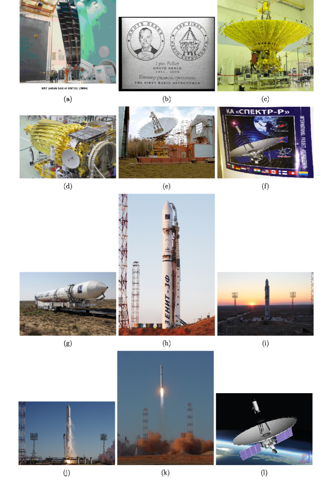
Figure 4: (Color inset 1). See full caption on a separate page below.

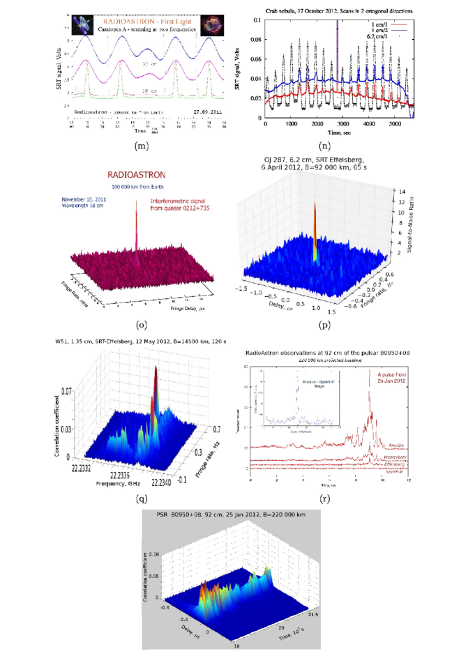
Figure 7: (Color inset 2). See full caption on a separate page below.

Figure 4 (color inster 1) caption:
(a) Tests of the precision carbon-fiber panels of the radio-telescope reflector at ESTEC in 1994 (Nordwijk, the Netherlands). (b) Memorial plate with a portrait of the first radio astronomer Grote Reber (1911–2002) mounted on the SRT. (c,d) Final ground tests of the SRT with the Navigator module were carried out at the Lavochkin Association right up to the transport of the spacecraft to the cosmodrome. Panel (d) shows the antenna of the SRT in the folded state; the 1.5-m antenna of the HDRRC and some of the solar panels are also visible. (e) Tests of a model of the SRT and interferometer at the PRAO (ASC) in 2003–2004. (f) Image of the SRT with logos of the organizations and flags of the countries participating in the RadioAstron project on the rocket fairing of the Zenit-3F complex. (g)–(h) Transport of the rocket with the Spektr-R spacecraft and the Fregat booster at the launch pad of site No. 45 of the Baikonur cosmodrome. (i) Launch on July 18, 2011 at 5:31:19.91 Moscow daylight savings time. (j) Artist’s impression of the SRT in orbit after it had successfully deployed on July 23, 2011.

Figure 7 (color inset 2) caption:
(a) Radiometric responses of the telescope during the first observation of the radio source Casseoipeia A with the SRT in flight, on September 27, 2011, at 92 and 18 cm in left- and right-circular polarizations. The two scans to the left were made for one cut through the source (in the forward and reverse directions), the two scans to the right were made perpendicular to this but, and the middle scan shows a cut through the edge of the object made during repointing of the antenna. The short pulses are responses to calibration signals from the receivers. (b) Example of radiometric responses of the SRT to a source during scanning of a portion of sky containing the Crab Nebula simultaneously at two wavelengths — 1.35 cm (in both polarizations) and 6.2 cm (in one polarization) — for observations with the SRT in a single-dish regime obtained on October 17, 2011. (c) First signal obtained at the ASC from the space–ground radio interferometer at 18 cm, for observations of the quasar 0212+735 made by the SRT and the 100-m Effelsberg radio telescope (Germany) on November 15, 2011. (d) Response of the space–ground interferometer (in units of the signal-to-noise ratio) for 6.2-cm observations of the quasar OJ287 on April 6, 2012. The projected baseline between the SRT and Effelsberg was $B=7.2$ Earth diameters. (e) Interferometer response for observations of narrow water lines at 1.35 cm in maser sources in the star-forming region W51 obtained for observations made by the SRT and the Effelsberg telescope on May 12, 2012. The projected baseline is $B=1.14$ Earth diameters (14 500 km), corresponding to an angular resolution of about 0.0002 arcsec. The integration time was 120 s. The vertical axis plots the correlation coefficient for the interferometer response as a function of the observing frequency and the fringe rate. (f) Four-antenna interferometric observations of a single pulse from the pulsar PSR B0950+08 made on January 25, 2012, involving the SRT and the Arecibo (Puerto Rico, USA), Westerbork (Netherlands), and Effelsberg (Germany) ground radio telescopes. The projected baseline is 220 000 km. (g) Same as (f) for the accumulation of a long series of pulses. The variation of the signal with time over an hour is clearly visible.

References

- (1) L. I. Matveenko, N. S. Kardashev, and G. B. Sholomitskii, Soviet Radiophys. 8, 461 (1965).
- (2) N. S. Kardashev, Yu. N. Pariiskii, and N. D. Umarbaeva, Astrofiz. Issled. 5, 16 (1973).
- (3) V. I. Buyakas, A. S. Gvamichava, L. A. Gorshkov, G. A. Dolgopolov, Yu. I. Danilov, M. B. Zakson, N. S. Kardashev, V. V. Klimashin, V. I. Komarov, N. P. Mel’nikov, G. S. Narimanov, O. F. Prilutskii, A. S. Pshennikov, V. G. Rodin, V. A. Rudakov, A. I. Savin, R. Z. Sagdeev, Yu. P. Semenov, A. G. Sokolov, V. I. Usyukin, K. P. Feoktistov, G. S. Tsarevskii, and I. S. Shklovskii, Kosmich. Issled. 16, 767 (1978).
- (4) N. W. Broten, T. H. Legg, J. L. Locke, et al., Science 156, 1592 (1967).
- (5) C. Bare, B. G. Clark, K. I. Kellermann, et al., Science 157, 189 (1967).
- (6) K. I. Kellermann, B. G. Clark, C. C. Bare, et al., Astrophys. J. Lett. 153, L209 (1968).
- (7) J. Gubbay, A. J. Legg, D. S. Robertson, et al., Nature 222, 730 (1969).
- (8) K. I. Kellermann, D. L. Jauncey, M. H. Cohen, et al., Astrophys. J. 169, 1 (1971).
- (9) D. D. Broderik, V. V. Vitkevich, D. L. Dzhonsi, et al., Sov. Astron. 14, 627 (1970).
- (10) L.I. Matveenko, Soobshch. IPA RAN No 176 (Inst. Prikl. Astron. RAN, St. Peterburg, 2007).
- (11) T. J. Pearson and A. C. S. Readhead, Astrophys. J. 328, 114 (1988).
- (12) Y. Y. Kovalev, K. I. Kellermann, M. L. Lister, et al., Astron. J. 130, 2473 (2005).
- (13) N. S. Kardashev, Yu. N. Pariiskii, and A. G. Sokolov, Usp. Fiz. Nauk 104, 328 (1971).
- (14) M. B. Zakson, N. S. Kardashev, A. I. Savin, et al., Zemlya Vselennaya, No 4, 2 (1980).
- (15) V. M. Arsent’ev, V. I. Berzhatyi, V. A. Blagov, et al., Sov. Phys. Dokl. 27, 362 (1982).
- (16) Astro Space Center, Lebedev Physical Institute, http://www.asc.rssi.ru/
- (17) G. S. Levy, R. P. Linfield, C. D. Edwards, et al., Astrophys. J. 336, 1098 (1989).
- (18) R. P. Linfield, G. S. Levy, C. D. Edwards, et al., Astrophys. J. 358, 350 (1990).
- (19) H. Hirabayashi, H. Hirosawa, H. Kobayashi, et al., Science 281, 1825 (1998).
- (20) H. Hirabayashi, H. Hirosawa, H. Kobayashi, et al., Publ. Astron. Soc. Jpn. 52, 955 (2000).
- (21) V. V. Khartov, Solar System Research, 46, 451 (2012).
- (22) Yu. A. Aleksandrov et al., Solar System Research, 46, 458 (2012).
- (23) Yu. A. Aleksandrov et al., Solar System Research, 46, 466 (2012).
- (24) Lavochkin Scientific and Production Association, http://www.laspace.ru/
- (25) RadioAstron User Handbook. http://www.ascrssi.ru/radioastron/documents/rauh/en/rauh.pdf
- (26) V. Yu. Avdeev, A. V. Alakoz, Yu. A. Aleksandrov, et al., Vestn. FGUP NPO im. S.A. Lavochkina, No 3, 4 (2012).
- (27) G. N. Zastenker, L. M. Zelenyi, A. A. Petrukovich, et al., Vestn. FGUP NPO im. S.A. Lavochkina, No 3, 22 (2012).
- (28) Yu. A. Aleksandrov, A. N. Kotik, N. V. Myshonkova, and S. D. Fedorchuk, in Radioastronomical Tools and Techniques, Ed. by N. S. Kardashev and R. D. Dagkesamanskii (Cambridge Scientific, Cambridge, 2007), p. 69.
- (29) I. S. Vinogradov, in Radioastronomical Tools and Techniques, Ed. by N. S. Kardashev and R. D. Dagkesamanskii (Cambridge Scientific, Cambridge, 2007), p. 49.
- (30) V. V. Andrejanov, L. I. Gurvits, N. S. Kardashev, et al., in QUASAT: A VLBI Observatory in Space, ESA SP-213 (European Space Agency, 1984), p. 161.
- (31) V. V. Andreyanov, A. V. Biriukov, V. I. Vasil’kov, et al., in Radioastronomical Tools and Techniques, Ed. by N. S. Kardashev and R. D. Dagkesamanskii (Cambridge Scientific, Cambridge, 2007), p. 17.
- (32) R. F.C. Vessot, M. V. Levine, E. M. Mattison, et al., Phys. Rev. Lett. 45, 2081 (1980).
- (33) P. Waller, F. Gonzalez, J. Hahn, et al., in Proc. 40th Precise Time and Time Interval Meeting (Reston, Virginia, USA, 2009), p. 69.
- (34) A. V. Biriukov, in Radioastronomical Tools and Techniques, Ed. by N. S. Kardashev and R. D. Dagkesamanskii (Cambridge Scientific, Cambridge, 2007), p. 57.
- (35) N. S. Kardashev, B. B. Kreisman, and Yu. N. Ponomarev, in Radioastronomical Tools and Techniques, Ed. by N. S. Kardashev and R. D. Dagkesamanskii (Cambridge Scientific, Cambridge, 2007), p. 3.
- (36) R. J. Eanes, B. Schutz, and B. Tapley, in Proc. 9th International Symposium on Earth Tides (E. Schweizerbart’sche VerlagBuchhandlung, Stuttgart, 1983), p. 239.
- (37) W. M. Folkner, J. G. Williams and D. H. Boggs, The Planetary and Lunar Ephemeris DE-421. JPL Memorandum IOM 343R08003 (2008).
- (38) F. G. Lemoine, S. C. Kenyon, J. K. Factor, et al., The Development of the Joint NASA GSFC and the National Imagery and Mapping Agency Geopotential Model egm96 (NASA, 1998). http://bowie.gsfc.nasa.gov/697/staff/lemoine/EGM96_NASA-TP-1998-206861.pdf
- (39) D. A. Duev, C. G. Molera, S. V. Pogrebenko, et al., Astron. Astrophys. 541, A43 (2012).
- (40) M. V. Sazhin, V. Yu. Vlasov O. S. Sazhina, and V. G. Turyshev, Astron. Rep. 54, 959 (2010).
- (41) I. E. Molotov, V. M. Agapov, V. V. Kupriyanov et al., Izv. Gl. Astron. Observ. Pulkovo 219 (1), 239 (2009).
- (42) IAU Minor Planet Center. http://www.minorplanet-center.net/iau/DASO/DASO.html
- (43) N. A. Esepkina, D. V. Korol’kov, and Yu. N. Pariiskii, Radio Telescopes and Radiometers (Nauka, Moscow, 1973) [in Russian].
- (44) A. R. Thompson, J. M. Moran, and G. W. Swenson, Jr., Interferometry and Synthesis in Radio Astronomy (Wiley, New York, 2001; Fizmatlit, Moscow, 2003).
- (45) Y. Y. Kovalev, N. A. Nizhelsky, Yu. A. Kovalev, et al., Astron. Astrophys. Suppl. Ser. 139, 545 (1999).
- (46) Yu. A. Kovalev, V. I. Vasil’kov, A. V. Biryukov, and N. Ya. Nikolaev, in Proceedings of the All-Russia Astronomical Conference (Spets. Astrofiz. Observ. RAN, Nizhnii Arkhyz, 2010), p. 32.
- (47) Report on Radio Astronomical Ground Tests of the SRT in Pushchino (AKTs FIAN, Moscow, 2004) [in Russian].
- (48) J. W. M. Baars, R. Genzel, I. I. K. Pauliny-Toth, and A. Witzel, Astron. Astrophys. 61, 99 (1977).
- (49) Institut of Radioastronomy of Max Plank (MPIFR, Bonn, Germany).
- (50) R. C. Hansen, Microwave Scanning Antenna (Academic, New York, 1964; Sov. Radio, Moscow, 1966), vol. 1.
- (51) G. Z. Aizenberg, UHF Antennas (Svyaz’, Moscow, 1957, 1977) [in Russian].
- (52) U. Christiansen, I. Hogbom, Radio Teleskopes (Cambridge Univ. Press, New York, 1969; Mir, Moscow, 1972).
- (53) G. K. Galimov, Reflector Scanning Antennas (Advansed Solutions, Moscow, 2010), Vol. 2 [in Russian].
- (54) Yu. V. Shubarin, UHF Antennas (Khar’kovsk. Univ., Khar’kov, 1960) [in Russian].
- (55) A. M. Tseitlin, Antenna Techniques and Radio Astronomy (Sov. Radio, Moscow, 1976) [in Russian].
- (56) Numerical Calculation of the SRT AFA Radiation Pattern at 1.35, 6.2 and 18 cm, Appendix to Design Documentation (ASC, Moscow, 2012) [in Russian].
- (57) A. D. Kuzmin and A. E. Salomonovich, Radioastronomical Methods of Antenna Measurements (Sov. Radio, Moscow, 1964; Academic Press, New York, 1966).
- (58) K. Hachisuka, A. Brunthaler, K. M. Menten, et al., Astrophys. J. 645, 337 (2006).
- (59) T. Hirota, T. Bushimata, Y. K. Choi, et al., Publ. Astron. Soc. Jpn. 59, 897 (2007).
- (60) T. Shimoikura, H. Kobayashi, T. Omadaka, et al., Astrophys. J. 634, 459 (2005).
- (61) A. Tolmachev, Astron. Tel. No. 3177 (2011).
- (62) E. E. Bloemhof, M. J. Reid, and J. M. Moran, Astrophys. J. 397, 500 (1992).
- (63) K. G. Belousov and S. F. Likhachev, in Radioastronomical Tools and Techniques, Ed. by N. S. Kardashev and R. D. Dagkesamanskii (Cambridge Scientific, Cambridge, 2007), p. 95.
- (64) A. R. Whitney, ASP Conf. Ser. 306, 123 (2003).
- (65) The RadioAstron Newsletter . http://www.asc.rssi.ru/radioastron/news/news.html
- (66) A. Wolszczan and J. M. Cordes, Astrophys. J. Lett. 320, L35 (1987).
- (67) M. J. Valtonen, H. J. Lehto, L. O. Takalo, and A. Sillanää, Astrophys. J. 729, 33 (2011).
- (68) K. I. Kellermann and I. I. K. Pauliny-Toth, Astrophys. J. Lett. 155, 71 (1969).
- (69) M. H. Cohen, M. L. Lister, D. C. Homan, et al., Astrophys. J. 658, 232 (2007).