Kinematics of Arp 270: gas flows, nuclear activity and two regimes of star formation

Abstract

We have observed the Arp 270 system (NGC 3395 & NGC 3396) in H$\alpha$ emission using the GH$\alpha$FaS Fabry-Perot spectrometer on the 4.2m William Herschel Telescope (La Palma). In NGC 3396, which is edge-on to us, we detect gas inflow towards the centre, and also axially confined opposed outflows, characteristic of galactic superwinds, and we go on to examine the possibility that there is a shrouded AGN in the nucleus. The combination of surface brightness, velocity and velocity dispersion information enabled us to measure the radii, FWHM, and the masses of 108 HII regions in both galaxies. We find two distinct modes of physical behaviour, for high and lower luminosity regions. We note that the most luminous regions show especially high values for their velocity dispersions and hypothesize that these occur because the higher luminosity regions form from higher mass, gravitationally bound clouds while those at lower luminosity HII regions form within molecular clouds of lower mass, which are pressure confined.

1 Introduction

The detailed effects of galaxy interactions on nuclear activity (Canalizo et al., 2007; Bennert et al., 2008; Georgakakis et al., 2009; Cisternas et al., 2011; Ramos Almeida et al., 2011, 2012; Bessiere et al., 2012) and also on star formation (Somerville et al., 2008; Bournaud, 2011; Tadhunter et al., 2011) demand considerable further study. The scaling relations showing the dependence of emission line widths in molecular clouds appear to be determined by supersonic turbulence (Blitz & Williams, 1999). Turbulence gives rise to density perturbations, locally triggering gravitational collapse, and leading to the formation of stars (Mac Low & Klessen, 2004; Klessen, 2011). But there is also evidence that magnetic fields play a role in controlling the collapse (Collins et al., 2012). The relative importance of these effects, in general, is not well understood, so that a variety of new observational results is needed to help clarify them. There is also evidence for the existence of triggered star formation. As pointed out by Bournaud (2011), the density is a parameter which is important in determining how the stars form, so that if we have sets of placental clouds with different density regimes we might well expect distinct star formation regimes within them. We have initiated a program of kinematic observations of interacting galaxy pairs analyzing the H$\alpha$ emission line, using an instrument which gives unequalled angular and velocity resolution per unit observation time. These observations, with the GH$\alpha$FaS Fabry-Perot 2D spectrometer on the 4.2m William Herschel telescope, allow us, inter alia, to explore a part of HII region parameter space normally not attainable in all but the most massive single galaxies: that of the most luminous regions (in galaxies of lower mass such a study is limited by low number statistics). They also allow us more generally to gain insights into how the dynamical effects demonstrated by the kinematic disturbances affect properties such as the presence of an AGN, and the overall SFR. A set of results for the weakly interacting pair in the Arp 271 system have recently been presented (Font et al., 2011), in which gas transfer detected between the two galaxies could be quantitatively related to an enhanced SFR and a nuclear wind in one of them. In the present article we present our observations of the Arp 270 system, which contains an apparently almost face-on galaxy, NGC 3395, and an almost edge-on galaxy, NGC 3396 (Figure 1), and which has reached a phase of closer interaction than the galaxies in Arp 271.

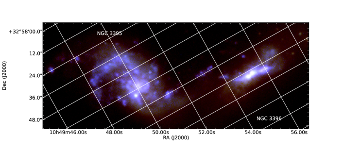
Figure 1: Composite colour map of Arp 270 from SDSS images. In this figure, and in all subsequent figures with images of Arp 270, the coordinates axes are those displayed explicitly in this figure.

The distance to Arp 270 is $21.8\,\mathrm{Mpc}$ (Tully, Shaya, & Pierce, 1992), yielding a scale of $0.1\,\mathrm{kpc}\,\mathrm{arcsec}^{-1}$. The systemic velocities of NGC 3395/6 are $1605\,\mathrm{km}\,\mathrm{s}^{-1}$ and $1675\,\mathrm{km}\,\mathrm{s}^{-1}$ while the inclinations are $50^{\circ}$ and $70^{\circ}$ respectively (Garrido et al., 2002).

Arp 270 is an approximately equal-mass merger (mass ratio 1.5:1) thought to be at its 2nd approach, e.g. Clemens et al. (1999), its star formation rate remainS moderate ($L_{FIR}\lesssim 10^{44}\,\mathrm{erg/s}$ (Sanders et al., 2003), thus $SFR\lesssim 5\,\mathrm{M_{\odot}/yr}$) but is probably due to increase at the forthcoming pericenter since it is in a pre-starburst rather than post-starburst condition.

In section $\S 2$ we explain the observations and the calibration method used. In section $\S 3$ we present an analysis of the global kinematics, focusing on the most interesting case of NGC 3396 plus the possibility that there is an AGN in it, which may be fed by the interaction. In section $\S 4$ we show the physical properties inferred for the HII regions in the galaxies, with evidence of two physically distinct populations. We also offer suggestions for the origin of the two regimes. In section $\S 5$ we give a discussion and present conclusion.

2 Observations & H$\alpha$ Calibration

The observations were taken on the night of December $23^{rd}$, 2010, with GH$\alpha$FaS (Galaxy H$\alpha$ Fabry-Perot Spectrometer, Hernandez et al. (2008), Fathi et al. (2008)) , at the Nasmyth Focus of the 4.2m William Herschel Telescope, ORM (La Palma). The spectrometer has a circular FOV with a diameter of 3.5 arcmin. In H$\alpha$, the etalon used covers a Free Spectral Range (FSR) of 8$\,\mathrm{\AA}$ which corresponds to 390 km/s with a spectral resolution $\delta\lambda$ of 0.2$\,\mathrm{\AA}$ which corresponds to a velocity resolution $\delta v$ of some 8 km/s. The pixel size of the detector subtends 0.2 arcsec on the sky, and the angular resolution was seeing limited at around 1 arcsec or 0.1 kpc on the galaxy assuming a distance of 21.8 Mpc. As the instrument operates at the Nasmyth focus, and GH$\alpha$FaS has not an optical derotator, the observations are affected by rotation of the field. However, GH$\alpha$FaS takes individual spectral scans covering the complete spectral range over the full field in only 8 min which allows us to use a digital derotation technique to bring all the scans into a uniform geometrical register. The technique has been described in Blasco-Herrera et al. (2010). After applying this correction, calibration in velocity, and phase adjustment we have a data cube to which we have applied the procedures described in Daigle et al. (2006) to derive maps of Arp 270 in H$\alpha$ surface brightness, velocity, and velocity dispersion, which are shown in Figure 2.

In order to calibrate the H$\alpha$ in flux we used the measured flux for the system obtained by Kennicutt et al. (2009) and compared it with the integrated photon count per second from GH$\alpha$FaS, $F_{G}$, once corrected for the specific filter transmittance, that is:

$$F_{H\alpha}\,\mathrm{(W/cm^{2})}=7.7\cdot 10^{-21}\thinspace F_{G}\,\mathrm{(counts/s)}$$ (1)

Although using the galaxies as a single object does entail some uncertainty, the results are consistent, within 10%, with those of Blasco-Herrera et al. in preparation (2013), and with calibrations performed on individual regions in M61 using the data from Knapen et al. (2004) and data observed with GH$\alpha$FaS.

$$F_{H\alpha}\,\mathrm{(W/cm^{2})}=8.6\cdot 10^{-21}\thinspace F_{G}-2.17\cdot 10^{-21}\,\mathrm{(counts/s)}$$ (2)

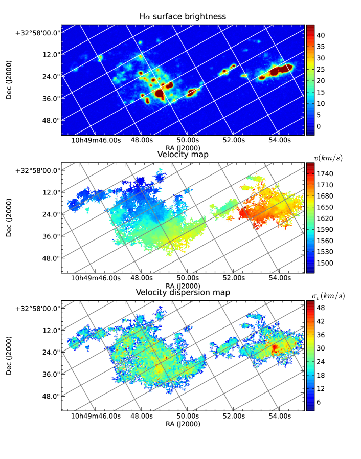
Figure 2: (From top to bottom: H$\alpha$ surface brightness; first moment map, giving the velocity fields of the two galaxies forming Arp 270; second moment map showing the velocity dispersion.

The previous flux calibrations ignore the effect of dust attenuation. Unfortunately, we are not be able to correct of dust attenuation for each region of the galaxies, but we can estimate the dust attenuation in each galaxy from their 1.4GHz luminosities given in Condon, Cotton, & Broderick (2002). Then, using the calibration of Kennicutt et al. (2009) (equation 12) to correct for dust attenuation using 1.4GHz luminosity, we have found that the global SFR for NGC3396 needs to be corrected by a factor of $2.3$ and NGC3395 needs to be corrected by a factor of $3.5$. However, as we study specific regions of the galaxies, we do not have the data to correct each of them for attenuation, so the values we give are lower limits to the SFR. It is significant that NGC3395 is more affected by dust attenuation than NGC3996 as we will comment below.

3 Global kinematics

The velocity map in Figure 2 shows a distorted rotation field in NGC 3395, and an apparently similarly distorted field in NGC 3396. However the velocity range in the latter case, $\Delta v\sim 80\,\mathrm{km/s}$, is much too small for an apparently edge-on galaxy with the mass which we have found in the literature (Clemens et al., 1999) of $\sim 2\cdot 10^{10}\,\mathrm{M_{\odot}}$ and calls for more detailed analysis which we present here. The velocity dispersion map in 2 shows quite high velocity dispersions (up to $\sim 50km/s$) and a correlation between the peaks of the velocity dispersions and the star-forming knots. We will present these aspects in more detail in section $\S 4$. These maps and the H$\alpha$ datacube are available through CDS.

Although the galaxies are clearly affected by the interaction, we have estimated the kinematical parameters using the velocity maps. We did this by using ADHOC software, written by J. Boulesteix, (Observatoire de Marseille), to optimize the circular velocity field. We show the results in Table 1, where we have included the calibration of H$\alpha$ in flux and the position angle (PA) is defined as “the counter-clockwise angle between north and a line which bisects the tracer’s velocity field, measured on the receding side” (Davis et al., 2011).

Object	$log(L_{H\alpha})\,\mathrm{(erg/s)}$	${Centre}_{kin}$ (RA;Dec)	$PA$ (∘)	$i$ (∘)	$v_{sys}\,\mathrm{(km/s)}$
NGC 3395	$41.34$	$10\,\mathrm{h}\thinspace 49\,\mathrm{m}\thinspace 50.31\,\mathrm{s}\thinspace\pm\thinspace 0.07\,\mathrm{s};\thinspace 32^{\circ}59^{\prime}00^{\prime\prime}\thinspace\pm\thinspace 1^{\prime\prime}$	$1\thinspace\pm\thinspace 6$	$59\thinspace\pm\thinspace 3$	$1600\thinspace\pm\thinspace 20$
NGC 3396	$40.99$	$10\,\mathrm{h}\thinspace 49\,\mathrm{m}\thinspace 55.30\,\mathrm{s}\thinspace\pm\thinspace 0.07\,\mathrm{s};\thinspace 32^{\circ}59^{\prime}26^{\prime\prime}\thinspace\pm\thinspace 1^{\prime\prime}$	$286\thinspace\pm\thinspace 6$	$67\thinspace\pm\thinspace 4$	$1690\thinspace\pm\thinspace 40$

Table 1: Kinematic parameters.

3.1 Gas inflow towards the nucleus of NGC 3396

It is well known that interactions between galaxies can induce inflows of gas towards their centres (see e.g. Mihos & Hernquist (1996)). We can see from the H$\alpha$ surface brightness map in Figure 2 that there is a powerful source of emission in the central zone of NGC 3396. This leads directly to a possible explanation for the low range of “rotational“ velocities detected in this galaxy: they are not in fact rotational, but projected inflow velocities along what appears to be a bar. Since NGC 3396 was classified as a barred galaxy by de Vaucouleurs et al. (1991) so we do not need to claim the presence of a bar but the non-rotational velocities. In order to test this scenario we have combined the H$\alpha$ surface brightness and velocity information by plotting their values around elliptical loci, which are the projections on the sky of circular orbits. An example is shown in Figure 3, where the velocity gradient is enhanced as we cross the bar; on one side the velocity component towards us decreases, and that towards the nucleus increases, and on the other side the effect is reversed.

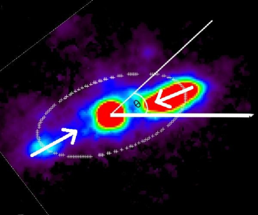
Figure 3: H$\alpha$ surface brightness (top-right) and radial velocity (bottom-right) plotted in an ellipse (left) around the nucleus

This behaviour is detected along the whole length of the bar. The velocity profiles are strongly reminiscent of the simulated profiles in Athanassoula (1992), in which gas is shocked as it collides with the bar, forming dust lanes, with their characteristic morphology.

On the assumption that we can derive the underlying kinematic parameters using the distorted velocity map of NGC 3396, we then went on to obtain the non-circular component, which in this case is the inflow velocity. We have subtracted off the rotation field obtained while estimating global kinematics parameters (Table 1) from the observed field, to yield a map of the residual, non-circular velocities.

Figure 4: Left, non-circular velocity map of NGC3396, the ”X” mark represents the kinematic nucleus. Right, dust lane model from Athanassoula (1992)

The resulting map is shown Figure 4, where the negative components of the non-circular motion (blue regions) to the left of the kinematic nucleus, and the positive components (yellow regions) to the right of the nucleus have the shape of typical curved dust lanes observed in barred galaxies (Athanassoula, 1984). We have been able to make a zero order estimate of $\phi$, the ionized gas mass inflow rate, using the approximation $\phi=2\cdot\rho\cdot\sigma\cdot v$. In this expression $\rho$ is the ionized gas density, which we have estimated using the mean luminosity-weighted electron density, hereinafter for simplicity called electron density, $n_{e}=<n_{e}>$; $\sigma$ is the cross section of the inflow along the bar, and $v$ is the velocity directed towards the nucleus. We have incorporated a factor 2 to take into account the flow along both sides of the bar. Because of the geometry of NGC 3396, to one side of the bar what we first see in the line of sight is the dust (blue regions in Figure 4). Thus, we are able to observe the geometry on this side of the bar and this is the side we have used to estimate the velocity of the inflow and the diameter of an idealized cylinder where the inflow occurs. However, as the dust is absorbing the H$\alpha$ emission, we have to estimate the electron density from the other side of the bar, where the star formation is seen before the dust in the line of sight.

Following Relaño et al. (2005) we can measure the electron density, $n_{e}=\rho$, using the H$\alpha$ luminosity and an estimate of the dimensions of the emitting region. If we consider spherical HII regions composed only by hydrogen with uniform density (Spitzer, 1978):

$$\frac{L_{H\alpha}}{\pi R^{2}}=h\nu_{H\alpha}\alpha_{H\alpha}^{eff}(H_{0},T)2.46\cdot 10^{17}\cdot n_{e}^{2}R$$ (3)

where $\alpha_{H\alpha}^{eff}(H_{0},T)$ is the effective recombination coefficient of the $H\alpha$ emission line, $h\nu_{H\alpha}$ is the energy of an $H\alpha$ photon and R is the radius in cm of the HII region.

We estimate $n_{e}$ from the value of the electron density found in the approaching part of the bar in section §4 yielding $\rho=n_{e}=4.2\,\mathrm{e^{-}/cm^{3}}$.

From the non-circular velocity map, we estimate the cross section diameter using the limits to the zone where the non-circular velocity is less than -10 km/s (since the uncertainty in our velocity measurements is $~{}8\,\mathrm{km/s}$), which yields an approximate value of $D=(300\pm 100)\,\mathrm{p}c$.

If $(r,\Phi)$ and $(R,\theta)$ are the polar coordinates in the sky and galaxy planes respectively, the $v_{los}$ can be written (van der Kruit & Allen, 1978)

$$v_{los}=v_{\theta}\thinspace sin\thinspace i\thinspace cos\thinspace\theta+v_{R}\thinspace sin\thinspace i\thinspace cos\thinspace\theta$$ (4)

where $v_{\theta}$ and $v_{R}$ are the circular and the radial velocity (velocity towards the nucleus, $v_{in}$, in our case) respectively. The relation between the galaxy and sky coordinates is:

$$tg\thinspace\theta=\frac{tg\thinspace(\Phi-\Phi_{0})}{cos\thinspace i}$$ (5)

$$R=\frac{r\thinspace cos\thinspace(\Phi-\Phi_{0})}{cos\thinspace\theta}$$ (6)

As we already have removed the circular velocity, $v_{\theta}=0$ for the residual map (Figure 4). Then, $v_{R}$ projected in the line of sight, $v_{los}$, is the one we can measure in the residual map. We estimate $v_{los}$ and $\Phi-\Phi_{0}$ using the side of the bar where the line of sight first mets the dust, as in our estimate of the diameter.

The mean value of the $v_{los}$ for the points where $v_{los}>10\,\mathrm{km/s}$ is $<v_{los}>=(17.0\pm 4.0)\,\mathrm{km/s}$. The result for the angle between the bar and the kinematic position angle is $<\Phi-\Phi_{0}>=(27\pm 8)^{\circ}$ and the inclination obtained in the determination of the rotation curve, $i=(67\pm 4)^{\circ}$, implying $\theta=(47\pm 15)^{\circ}$. Combining the previous results with equations 4, 5 and 6 we obtained an inflow velocity of $v_{in}=(27\pm 15)\,\mathrm{km/s}$.

The ionized gas inflow rate result is a value for $\phi$ of $(0.4\pm 0.2)\,\mathrm{M_{\odot}/yr}$, along the bar. From the H$\alpha$ emission in the circumnuclear zone, using the calibration of Kennicutt et al. (2009) we find a star formation rate of $0.15\,\mathrm{M_{\odot}/yr}$. These two values are mutually consistent: there appears to be enough inflow to fuel the circumnuclear star formation.

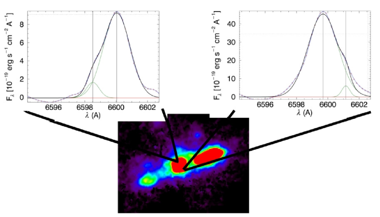
Figure 5: H$\alpha$ profile in opposite sides of the nucleus of NGC 3396

3.2 Outflow from the nucleus of NGC 3396

H$\alpha$ line profiles obtained in our GH$\alpha$FaS data present a variety of shapes showing multiple peaked profiles close to the nucleus (see Figure 5). The position of the secondary peak with respect to the main peak shifts as we change position around the nucleus, and the form of these shifts can be explained naturally in terms of a biconical outflow in a direction perpendicular to the plane of the inflow. This is similar to previous studies by Chatzichristou, Vanderriest, & Lehnert (1998) who found biconical outflow from a central bar-like structure in the interacting galaxy UGC 3995, as well as evidence for inflow along the bar, and by Veilleux, Shopbell, & Miller (2001), who found a biconical outflow from the AGN of NGC 2992.

Due to the small separation between components a simple multiple gaussian fit does not work without a proper values for initial parameters (the solution is strongly dependent on the initial values).

In order to effect best fits of multiple Gaussians to the profiles illustrated in Figure 6 we first approximated the parameters of the Gaussians, in order to restrict them to within the reasonable limits needed to obtain a convergent solution.

We have developed a method to find these approximations and their ranges using information derived from the first and second derivatives of the line profiles (Goshtasby & O’Neill, 1994).

Figure 6: H$\alpha$ profile (black), its first and second derivatives (red and blue, respectively). The vertical lines are the intersections of the maximum and minimum of the first derivatives and the zeros in the second derivatives.

In Figure 6 we show profiles with structures whose basic shapes are repeated from positions over the whole circumnuclear zone, so that we can safely eliminate the possibility that they are noise. We assume that the line structures are composed of separate individual contributions which need to be separated. Although there are no well resolved peaks, we can clearly see the change in the profile gradients, which allows us to use these to effect the separation of the lines. For an emission profile with two intrinsic components, if we consider the profile behaviour as the wavelength $\lambda$ increases the centre of the first component will lie between the first maximum and the first minimum of the first derivative of the profile, i.e. between the corresponding two zeros in the second derivative, (see Figure 6). The centre of the second component will lie between the maximum and minimum of the first derivative in the other half of the profile, i.e. between the corresponding zeros in the second derivative. This gives us a range of $\lambda$ for the centre of each of the two emission components, and the initial estimates of the line centres are made by taking the centre wavelengths of these ranges. Similarly the ranges give us initial estimates of the line widths, $\sigma_{v}$. We can then apply a standard Gaussian fitting routine with two components to a given observed profile, using the initial estimates as our starting points.

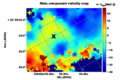
Figure 7: Left: main component velocity map. Right: velocity map of the outflow. The ”X” mark represents the kinematic nucleus.

The results of this method applied to the circumnuclear gas in NGC 3396 is shown in Figure 7, where we show the velocity distributions of the components detected to either side of the nucleus, as seen clearly using the colour coding. These maps were made using the main (Figure 7 left) and the secondary (Figure 7 right) components of the line profiles. From the angular distribution of the secondary component (Figure 7 right), we argue that there are two independent velocity components around the nucleus very different from the typical inflows patterns (spirals and/or bars) and from the velocity distribution we argue that the two velocity components are in opposite senses from the nucleus since the discontinuity in velocity is $~{}120\,\mathrm{km/s}$ around the kinematical nucleus. We suggest that it represents a biconical outflow of ionized gas from the nucleus of NGC 3396 rather than an inflow prolongation. Using a method for estimating the mass outflow rate which is analogous to that described in Section $\S 3.1$, we estimate the density as the electron density of the central region of $n_{e}=0.1\,\mathrm{e^{-}/cm^{-3}}$. We have used the $5\%$ of the $H\alpha$ luminosity in the central region since in the previous multiple components fit, we found that the outflow emits the $5\%$ of the total $H\alpha$ luminosity in the nucleus.

In order to estimate the section where the outflow occurs, we assume that the outflow is happening in a cylinder with radius equal to the radius of the base where the approaching and the receding part of the outflow join in Figure 7 (right), yielding a value of $R=(300\pm 100))\,\mathrm{pc}$. We assume that the velocity of the outflow is the deprojected (perpendicular to the disc plane, $i=(67\pm 4)^{\circ}$) mean value of the absolute velocity values in Figure 7 (right), yielding $v_{out}=(150\pm 50)\,\mathrm{km/s}$

We derive a value for $\phi$ , the outflow rate, of $(0.22\pm 0.07)\,\mathrm{M_{\odot}/yr}$.

The net difference between the inflow and outflow rates approximately coincides with the estimated SFR.

3.3 Interaction-induced nuclear activity?

We think that the interaction has induced nuclear activity, in particular star formation and, maybe, a shrouded AGN. The outflow is found in the NGC 3396 central ionized zone where $L_{H\alpha}=2.8\cdot 10^{40}\,\mathrm{erg/s}$. The majority of the H$\alpha$ luminosity is due to a burst of star formation that we have estimated as $0.15\,\mathrm{M_{\odot}/yr}$ since we have found that the outflow emits only $5\%$ of the H$\alpha$ luminosity. The outflow is maybe due to the winds of the massive stars that are forming in the nucleus. However, although the morphology of the outflow is not precisely determined, the overall shape does seem to correspond to the biconical effect expected from an AGN, even though it is not classified as such. We have checked the possibility that there is an obscured AGN, finding that Brassington, Read, & Ponman (2005) did discover an X-ray source close to the H$\alpha$ nucleus, whose spectral hardness and luminosity could imply an origin in an AGN.

We therefore extracted its X-ray spectrum from the Chandra data archive to look for indicators of the presence of AGN in this range. Unfortunately, the hard band (2-10 keV) presented very few counts and therefore we could not detect the [Fe K] lines which are the main indicator with acceptable certainty, though we did find an excessively prominent [Si XIII] line in the soft band (0.5-2 keV) at 1.84 keV (Figure 8). The soft band was fitted with a line and continuum emission with tunable abundances model VMEKAL, initially assuming an abundance scheme derived from type II supernovae core collapse enrichment. This model failed to properly fit the [Si XIII] line by a factor of $\sim 12$ in the model parameter, meaning the abundance needed to fit the line is $\sim 12$ times that predicted by the SNII model. It has been found in a previous paper (Iwasawa et al., 2011), in a sample of 44 galaxies, that this excess, of at least twice, shows a good correlation with the presence of an AGN.

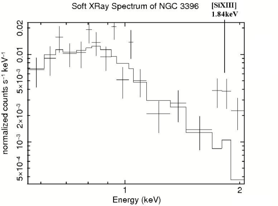
Figure 8: Observed Soft X-Ray spectrum of NGC 3396 (points) and the VMEKAL model of the observed spectrum (continuous line).

Satyapal et al. (2008) argue that the presence of strong ionization lines such us [NeV] at $14.3\,\mathrm{\mu m}$ and $24.3\,\mathrm{\mu m}$, or maybe [OIV] at $26.0\,\mathrm{\mu m}$, is strong evidence for an obscured AGN. We have analyzed infrared spectra from Spitzer of the nucleus of NGC 3396 but we did not find any strong ionization line supporting the evidence for an AGN, so the question remains open.

The overall result of the use of kinematic evidence to study the bar and circumnuclear zone of NGC 3396 is, then, to attribute the underlying velocity field to gas inflow to the nucleus rather than to rotation, to discover evidence for biconical outflow from the nucleus, and to detect symptoms of nuclear activity, star formation and/or a shrouded AGN.

4 Physical properties of HII regions

Using the H$\alpha$ emission from the two galaxies we can compare the SFR s (estimated from Kennicutt et al. (2009) as in section $\S 3.1$) in their circumnuclear zones with those in the external parts of the two galaxies. For NGC 3396 the circumnuclear SFR is $0.15\,\mathrm{M_{\odot}/yr}$, while in the rest of the disc the integrated SFR is $0.39\,\mathrm{M_{\odot}/yr}$. The corresponding figures for NGC 3395 are $0.08\,\mathrm{M_{\odot}/yr}$ and $1.1\,\mathrm{M_{\odot}/yr}$ respectively. Although we might think that the difference in the SFR s between the discs and the centres could be because NGC 3396 is edge-on, this is not evident, as we have found that the kinematics of this object are not those characteristic of an edge-on disc. If NGC3396 were edge-on, it would be more affected by dust. However, we have seen in section $\S 2$ NGC3395 is more affected by dust attenuation than NGC3396.

In order to explore these different SFR’s values in more depth we derived the directly observable physical parameters of the HII regions: the H$\alpha$ luminosity, $L_{H\alpha}$, the effective radius, $R$, and the velocity dispersion, $\sigma_{v}$ , from the GH$\alpha$FaS data cube, using the clumpfind algorithm (Williams, de Geus, & Blitz, 1994). We were careful to take into account the limitations of clumpfind (Pineda, Rosolowsky, & Goodman, 2009), estimating the completeness limits in order to obtain results unbiased by sensitivity and resolution considerations. We used a lower limit of 9 for the number of pixels per statistically significant region, and eliminated pixels from the regions selected which had S/N ratios less than 2. These two criteria set a lower limit for the luminosity of $L_{H\alpha\thinspace min}=18\,\mathrm{rms}=2\cdot\,\mathrm{rms}\cdot\pi\cdot R_{min}^{2}$, where rms is the rms noise level in the background of the H$\alpha$ signal. Another lower limit we have used is a lower limit in the non-thermal velocity dispersion, $\sigma_{v-nt}$, in $8\,\mathrm{km/s}$, the uncertainty in our velocity measurements, since we are going to use it to estimated the virial mass. We described the non-thermal velocity dispersion estimation bellow (section $\S 4.2$).

We made statistically valid measurements on 108 HII regions, 20 of which belong to NGC3996 and 88 to NGC3395.

We found results comparable to those obtained by Gutiérrez, Beckman, & Buenrostro (2011) who used narrow band imaging observations in H$\alpha$ surface brightness to determine the radii and luminosities of HII regions in M51. The additional dimension of velocity we use here serves to yield less scatter in the physical properties of the regions, as it reduces significantly the effect of confusion in the sources. Using the simplifying assumption of sphericity for the regions, we can obtain the mean electron density $n_{e}$ (in fact the luminosity-weighted electron density $<n_{e}>$, equation 3), and hence estimate the ionized hydrogen mass ($M_{HII}$) of each region. In section $\S 4.4$ we will describe how we have estimated the fraction of the ionized gas compared with the neutral atomic plus the molecular gas, and why it seems approximately constant, at least for the regions with $L_{H\alpha}>10^{38.7}\,\mathrm{erg/s}$. Using the ionization fraction of $0.2$ we have then estimated the total gas mass, $M_{gas}$ (ionized + neutral + molecular).

We also derived the virial mass of each region following Wei, Keto, & Ho (2012), using the expression they used assuming self-gravitating region in virial equilibrium,

$$M_{vir}=\frac{3\thinspace R\thinspace\sigma_{v-nt}^{2}}{G}$$ (7)

where $R$ is radius of the region we have measured.

We present the results of the physical properties in Tables 2, 3 and 4

4.1 Parameter analysis

Figure 9 (left panel) presents the comparison of $M_{vir}$ and $M_{gas}$, showing that the gas masses of the regions are generally lower than the virial masses, although there is a clear correlation between them. In Figure 9 (right panel) we show the luminosity function of the HII regions. There is an apparent break in the function at 38.6 dex, although we cannot claim accurate information here, because it is not easy to specify the lower completeness limit. We note that a break at this luminosity was first detected by Kennicutt, Edgar, & Hodge (1989); a more detailed study involving 57 galaxies was produced by Bradley et al. (2006), while Beckman et al. (2000) claimed that this break was due to a change from luminosity-bounded (in the lower luminosity regime) to a density-bounded regime (in the higher luminosity regime). However here we have the extra parameter of velocity dispersion which can give us further insights.

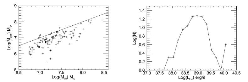
Figure 9: Left: Comparison between gas mass and virial mass. Right: luminosity function of the HII regions

4.2 Two populations of HII regions

A first step in our analysis involved plotting the mean electron density $n_{e}$ against the radius $R$ of the region, and also the H$\alpha$ luminosity, $L_{H\alpha}$ against $R$, as shown in the upper panels of Figure 10. Although it is possible to fit a non-linear curve with continuous change in slope to the latter, it is instructive to use the double linear fit shown in Figure 10 (upper right panel).

The selection of the points as “blue“ or “red“ was made using a division into two groups The separation between the groups is clearer in the electron density-radius plot than in the luminosity-radius plot since there are regions where the electron density falls with radius, and there are regions where the electron density rises with radius, (Figure 10 upper left) Thus, in order to chose the correct separation we have assumed that the two regimes are separated in electron density-radius space. It is possible that the boundary is less well-defined than we have imposed here, but we are not as concerned to find a precise boundary between the two populations as we are to study the collective properties of the two different populations, and there may be a minor degree of mixing between the two populations near the boundary. We will show below, using the geometrical distribution of the two sets of regions, why this is in practice unlikely. We have chosen the separation of the two populations by means of the $\chi^{2}$ minimization (in the electron density-radius space) and a double linear fit for several possible separations. The result is the less luminous set of HII regions show an index of 2.5, while the more luminous set shows an index of 3.8.

We find that there are 9 regions in the lower luminosity regime and 11 in the higher luminosity regime in NGC3396, and for NGC3395 the corresponding numbers are 49 regions in the lower luminosity regime and 39 in the higher luminosity one. The higher luminosity regions in NGC3396 emit 94% of the H$\alpha$ luminosity while for NGC3395 these regions emit 75%. If we scale the SFR as proportional to the H$\alpha$ luminosity (this is the only SFR tracer used here ) this would imply that the higher luminosity regime represents 94% of the SFR in NGC3396 and 75% of the SFR in NGC3395.

We have distinguished between these two regimes because the $n_{e}$ decreasing regime agrees qualitatively with the result reported in Gutiérrez & Beckman (2010) who found, in M51 (for over 2000 HII regions) and in NGC 4449 (for over 200 regions), that $n_{e}$ varies as $\frac{1}{R^{0.5}}$. In their samples there were very few regions with luminosities higher than 38.6dex so they were essentially looking at the equivalent of the lower luminosity set of regions we are observing in Arp 270. This is due to the intrinsic properties of the luminosity functions in the two galaxies they observed, which means that the upper luminosity population we observe here is not represented in their work. In Figure 10 (upper left panel) we see that there is a tendency of the high luminosity regions, in blue, to show an increase in $n_{e}$ with increasing radius, the opposite tendency, at least in qualitative terms, from that exhibited by the lower luminosity set. It is worth noting two additional points here. Firstly Gutiérrez & Beckman (2010) found not only the $\frac{1}{R^{0.5}}$ dependence mentioned above, but also a very clear dependence of $n_{e}$ on the galactocentric radius of the HII region, which they interpreted as showing that the regions in their sample were pressure bounded. We will return to this point later, but it is mentioned here because we are not in a position to include this dependence in our results. Not only do the distance and the orientations of the two galaxies make any estimate of galactocentric radius very inaccurate, but the interaction itself will certainly affect the pressure distribution which confines the HII regions. This is at least one of the reasons why the dependence of $n_{e}$ on radius shows so much scatter in Figure 10.

A second point is brought out in the lower panels of Figure 10 where we show the H$\alpha$ surface brightness of the individually reconstructed map for each individual region, indicating the locations within the galaxies of the HII regions whose parameters are plotted in the upper panels. All the regions plotted as blue points in the upper panels are found in concentrated zones around the centres of the two galaxies, and in the interaction zone. All the regions plotted as red points are found in more peripheral zones of the galaxies. The zones in the two lower panels are precisely complementary, and do not overlap. This purely geometrical separation could have been used to distinguish the two populations in the first place, and it can be used to give good support to the separation criterion we in fact used, based on the radius-electron density diagram.

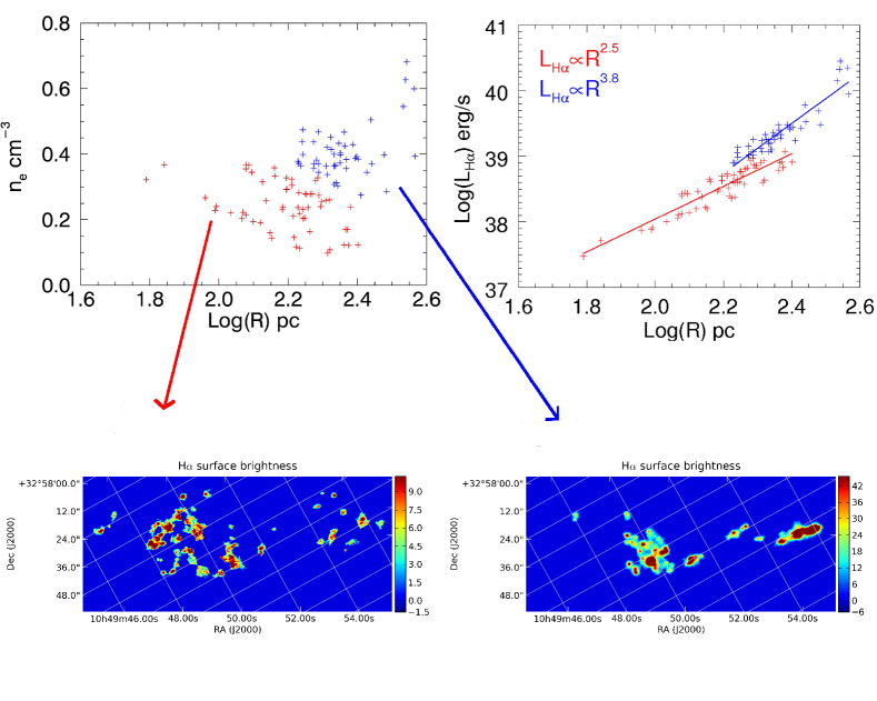
Figure 10: Relation between electron density, $n_{e}$, and HII region effective radius, $R$, (top-left). Relation between H$\alpha$ luminosity, $L_{H\alpha}$, and HII region effective radius, $R$ (Top-right). Red points are for the the decreasing $n_{e}$ regime and the red ones for the increasing one. Lower luminosity (bottom-left) and higher luminosity (bottom-right) HII regions.

The general dependence of the H$\alpha$ luminosity on the parameters of an HII region is analyzed via equation 3 where we neglected, for simplicity, the presence of helium and other elements, and if the hydrogen is fully ionized, equation 3 implies that the luminosity should depend simply on $R^{3}$ in case of $n_{e}$ were not R dependent. We have seen from Figure 10 that this relation does not hold, either for the lower luminosity regime, where the exponent is 2.5, or for the higher luminosity regime, where the exponent is 3.8. In the former case we can infer that $n_{e}$ must be a declining function of R, varying as $\frac{1}{R^{0.25}}$. This is not in good quantitative agreement with the results of Gutiérrez & Beckman (2010), but as explained above, we have not been able to disentangle the macroscopic effects of pressure variations within the galaxies for Arp 270. In the higher luminosity range, $n_{e}$ must vary as $R^{0.4}$, and this can be explained if the effect is due to the increasing ionization of the higher density clumps, as outlined above.

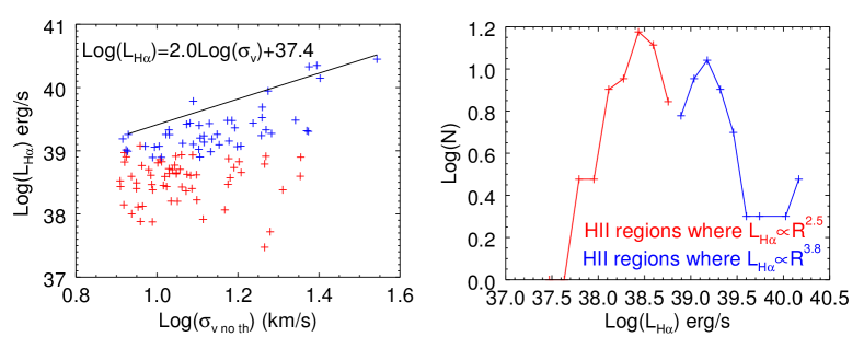
Figure 11: Relation between the H$\alpha$ luminosity, $L_{H\alpha}$, and the non thermal velocity dispersion, $\sigma_{v-nt}$, for each individual HII region. We have overlapped the fitted envelope, estimated following Relaño et al. (2005) (left). Luminosity function (right)

In Figure 11 (left hand panel), we have plotted $L_{H\alpha}$ against the non-thermal velocity dispersion, obtained from the observed velocity dispersion by subtraction in quadrature of the instrumental, thermal, and natural line widths. We have considered that the quadratic subtraction overestimates the non-thermal velocity dispersion in $~{}8\,\mathrm{kms^{-1}}$ (Blasco-Herrera et al., 2010), so we have subtracted it.

$L-\sigma$ relation for HII regions was first looked at in detail by Terlevich & Melnick (1981). They found that it could be expressed as a power law, $L\propto\sigma^{N}$, and suggested that N should take the value 4 for virialized regions. However in practice they, and subsequent studies, found values $N\in[1.0-6.6]$. Here we follow the method of Relaño et al. (2005) who suggested that points on the upper envelope in $L$ (the lower evelope in $\sigma$) should represent regions in virial equilibrium. Our result for this envelope is $Log(L_{H\alpha})=2.0\thinspace Log(\sigma_{v})+37.4$, which as we can see has a slope of 2 in Figure 11 left. In the last approach, the high luminosity regions tend to be more virialized (blue points in Figure 11 left) than the low luminosity regions (red points in Figure 11 left).

It is interesting to note how, as shown in Figure 11 (right hand panel), plotting the luminosity function separately for the HII regions in the two regimes gives an important clue to the origin of the discontinuity found in the undifferentiated luminosity function at $L_{H\alpha}=38.6\,\mathrm{dex}$.

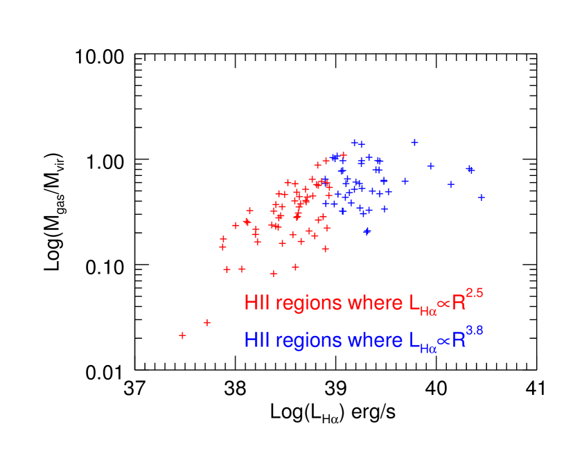
Figure 12: Total gas mass $M_{gas}$ over virial mass $M_{vir}$ versus $H\alpha$ luminosity for the higher luminosity regime (blue crosses) and lower luminosity regime (red crosses).

In Figure 12 we have plotted the ratio of the total gas mass to the virial mass. We note the tendency of this ratio to rise for larger radii, and higher masses for the regions in the lower luminosity regime. This is presumably because of the combination of two effects.

Firstly, the estimate of the total gas mass depends on the ionized gas mass due to the method we have used (described in $\S 4.4$) in estimating the total gas content for the lower luminosity regime. We argue that an increasing fraction of the hydrogen is ionized with increasing luminosity in this regime. Secondly, these regions are not virialized since they are bellow the envelope in the L-$\sigma$ relation (Figure 11 left), so the derived virial mass is in practice an overestimate of the gas mass.

However, there is a tendency for the gas mass to approach the virial mass for the higher luminosity regime. We can explain these observations qualitatively again, with a virialized scenario for HII regions for the higher luminosity regime since their gas masses approach parity with the virial mass.

4.3 Differences between the two regimes

Gutiérrez & Beckman (2010) showed that for the HII regions in M51 and NGC 4449 the decline in their values of $n_{e}$ with galactocentric radius, with scale lengths equal to the scale lengths of the HI surface densities in the two cases. This implies that the regions are in pressure equilibrium with the surrounding gas in the discs, and are in consequence pressure bounded. However, in Gutiérrez, Beckman, & Buenrostro (2011) it was noted that in both of these galaxies the number of regions with luminosities greater than $L_{H\alpha}=38\,\mathrm{dex}$ is small, with a complete absence of regions with luminosities greater than 39 dex. The difference between Arp 270 and these other objects seems to be that the interaction has stimulated the production of HII regions with luminosities higher than 39 dex, which are those in the high luminosity regime (regime 2) in the present article. So how can we account for the differences between the two regimes. One clue can be found in two articles dealing with another well-known pair of interacting galaxies: the Antennae. In Wei, Keto, & Ho (2012) and in Font et al. in preparation (2013) the authors detect two populations of giant molecular clouds, with a division between them at a cloud mass of $10^{6.5}\,\mathrm{M_{\odot}}$. This is close to the value of the gas mass which marks the change from regime 1 to regime 2 in Arp 270, and Font et al. in preparation (2013) have detected two equivalent regimes in the HII regions of the Antennae. These results lead us to postulate that the HII regions in regime 2 (high luminosity) are those which have formed in molecular clouds of high mass, which have own ”regime 2“, while the HII regions in regime 1 (low luminosity) have formed from molecular clouds in its ”regime 1“. We argue that while the HII regions in regime 1 are pressure bounded, those in regime 2 are gravitationally bound, (and bounded). Those with virial masses close to the upper envelope of the plot in Figure 9 (left panel) we will take as in virial equilibrium, and therefore gravitationally bound implying that the line widths of those regions are largely due to gravitation.

Further evidence supporting the idea of gravitationally bound regions can be found by making an estimate of the Jeans mass ($M_{J}$) from the equation (5.47) of LABEL:2008gady.book.....B,

$$M_{J}=2.92\frac{v_{s}^{3}}{G^{3/2}\rho_{0}^{1/2}}$$ (8)

where $v_{s}$ is the speed of sound and $\rho_{0}$ is the density. We have assumed $v_{s}=\sigma_{v-nt}$ and $\rho_{0}=\frac{M_{gas}}{(4/3)\pi R^{3}}$.

The comparison between the Jeans mass and the total gas mass of each region yields a relation very similar to the plot of the comparison between total gas mass and virial mass (Figure 12), implying that for the higher luminosity regions gravity dominates the equilibrium ($M_{gas}\simeq M_{J}$) while the lower liminosity regions appear to be held in quasi-equilibrium by the external pressure of the surrounding gas column, given that $M_{gas}<M_{J}$ (see also Gutiérrez & Beckman (2010) who find a different argument for pressure equilibrium in the HII regions of M51, which fall in the low luminosity regime).

The turbulence within the regions is assumed to maintain the regions against collapse (and, more surprisingly, but factually, the same is true of the molecular clouds in the Antennae, where the turbulent line widths are large enough to give support against gravity).

Another possible cause of the two regimes could be the ages of the regions. As the star formation in galaxy mergers tends to occur in the central regions of the galaxies, one might argue that the difference in the regimes is due to a difference stages in the HII regions evolution in time. We have plotted the $H\alpha$ equivalent width versus $H\alpha$ luminosity for each HII region in Figure 13. Assuming a direct relation between $W(H\alpha)$ and the region age (Leitherer et al., 1999), we can conclude from Figure 13 that the difference between regimes does not seem to be related to the region’s ages. However, what we found in Figure 13 is that the youngest regions ($Log(W(H\alpha))>2.7$) belong to the overlap region between the two galaxies.

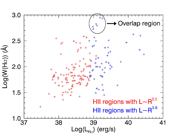
Figure 13: $H\alpha$ equivalent width ($W(H\alpha)$) versus $H\alpha$ luminosity ($L_{H\alpha}$)

We can add, somewhat speculatively, that if gravity is sufficiently dominant, the cloud could have a negative heat capacity (Lynden-Bell & Wood, 1968), so that a rise in temperature would cause it to contract. Under these conditions the injection of photoionization energy could cause a rise in density leading to enhanced star formation. Thus the two regimes may arise because of the differences between pressure bounded and gravity bounded molecular clouds, which in turn lead to differences in the dominant modes of star formation within them.

4.4 Results for global star formation.

Our observations allow us to show how the star formation rate surface density depends on the surface density of the gas. We can assume from the measurements we have made, that $L_{H\alpha}\propto R^{N}$ with $N=3.8$ is a good approximation for the high luminosity regions. Then, the mean electron density $n_{e}$ varies as $R^{\frac{N-3}{2}}$, obtaining expressions for the SFR surface density, $\Sigma_{SFR}$, and the ionized gas surface density $\Sigma_{ion\thinspace gas}$ in equation 9 and equation 10 respectively.

$$\Sigma_{SFR}\propto\frac{L_{H\alpha}}{R^{2}}\propto R^{N-2}$$ (9)

$$\Sigma_{ion\thinspace gas}\propto n_{e}\cdot R\propto R^{\frac{N-1}{2}}$$ (10)

Combining equations 9 and equation 10 we have

$$\Sigma_{SFR}\propto\Sigma_{ion\thinspace gas}^{\frac{2N-4}{N-1}}$$ (11)

and inserting the observed value of 3.8 for N we find that

$$N=3.8\rightarrow\Sigma_{SFR}\propto\Sigma_{ion\thinspace gas}^{1.3}$$ (12)

which shows that the HII regions in the high luminosity regime do obey the Kennicutt-Schmidt law for global star formation (Kennicutt, 1998). We can see this in Figure 14, where we show the values of the SFR surface density versus (ionized, in the case of Arp 270) gas surface density. In order to compare with the Kennicutt-Schmidt law, we show the values of normal galaxies, starburst galaxies taken from Kennicutt (1998) and the values of the M51 regions taken from Kennicutt et al. (2007).

The offset for the points from Arp 270 is due to the absence of measurements of the neutral and molecular gas components in the system. If we multiply per 5 the mass of the ionized gas, the offset would disappear, so we estimate the fraction of the ionized gas respect to the neutral plus molecular gas as $\sim 0.2$. This is the value we used to estimate the total gas mass, in section $\S 4$.

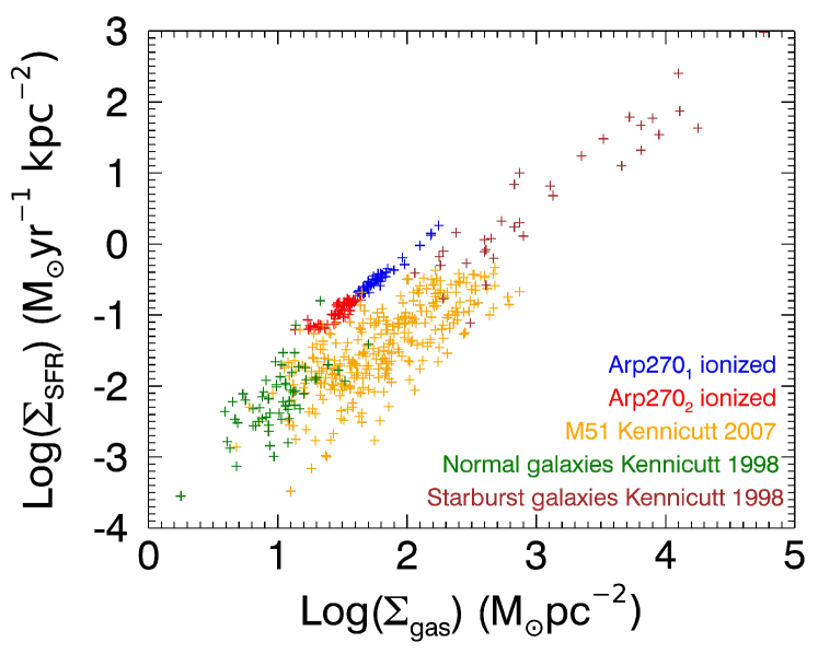
Figure 14: SFR Surface density versus (ionized in the case of Arp 270) gas surface density

5 Summary & Conclusions

We have shown that there is gas inflow along the bar of NGC 3396 at a rate of $(0.40\pm 0.2)\,\mathrm{M_{\odot}/yr}$, sufficient to maintain the observed star formation rate of $0.15\,\mathrm{M_{\odot}/yr}$. We have also detected a biconical gas outflow from the nucleus at a rate of $(0.22\pm 0.07)\,\mathrm{M_{\odot}/yr}$, and with velocities $150\pm 50\,\mathrm{km/s}$. If this outflow is generated by energy and momentum input from matter falling onto a supermassive nuclear black hole, it would take an inflow onto the black hole of only $4\cdot 10^{-5})\,\mathrm{M_{\odot}/yr}$ converted into kinetic energy and outflow momentum with an efficiency of 10% in order to fuel this superwind, so the hypothesis that the outflow detected indicates the presence of an AGN is relatively easy to sustain. We claim that this may show the presence of an interaction-induced nuclear activity, in the sense that the substantial mass inflow rate along the bar gives a straightforward mechanism for feeding the possible nuclear black hole, or the burst of star formation.

We have found two sets of HII regions in Arp 270, with a dividing line in H$\alpha$ luminosity at 38.7 dex. Those with high luminosity (regime 2) are found in zones closer to the centres of both galaxies, and in a specific interaction zone (the overlap region), while those in the lower luminosity regime (1) are found at larger galactocentric radii in the relatively less disturbed parts of the galaxy discs. The relations between the mean electron density $n_{e}$ and the radius of the region differ in the two regimes. We use arguments based on previous work to show that the regions in regime 1 are in pressure equilibrium with their surroundings, and argue that those in regime 2 are very probably gravitationally bound noting that the higher luminosity regions show especially high velocity dispersion values. This would favor a gravitationally triggered star formation scenario. The higher luminosity regime represents 94% of the SFR in NGC 3396, and 75% of the SFR in NGC 3395. The presence of a statistically significant sample of HII regions in regime 2 in NGC 3396 is surely due to the interaction between the galaxies, which has brought about inflow of gas towards their centers, and enhanced the density there and in limited regions of the discs which are in direct collision. However, for the existence of two star forming regimes of the kind we detect here galaxy galaxy interaction may well not be necessary. The evidence cited in the introduction for a change in slope of the luminosity function at $L_{H\alpha}=38.6\,\mathrm{dex}$ has been found previously in many galaxies, and the only condition appears to be the necessity for a sufficiently large number of HII regions at higher luminosities to be able to make statistically meaningful measurements of this function, and of the parameters we have measured in the present article, namely $n_{e}$, $\sigma_{v-nt}$, and $R$. The two basic conditions needed for this are either that the galaxy itself be sufficiently massive and gas rich to produce the appropriate population of placental molecular clouds, or that massive molecular clouds are produced during an interaction.

Appendix A HII regions properties

N	RA	Dec	R	$log(L_{H\alpha})$	$n_{e}$	$\sigma_{v-nt}$	$log(M_{HII})$	$log(M_{gas})$	$log(M_{vir})$
	(hh:mm:ss)	(∘ $\mathrm{\prime}$ $\mathrm{\prime\prime}$)	(pc)	$\,\mathrm{(}erg/s)$	$\,\mathrm{(}e^{-}/cm^{3})$	$\,\mathrm{km/s}$	$\,\mathrm{M_{\odot}}$	$\,\mathrm{M_{\odot}}$	$\,\mathrm{M_{\odot}}$
1	10 49 55.31	32 59 26.25	349	40.45	4.81	34.93	7.33	8.11	8.47
2	10 49 49.75	32 59 3.28	346	40.33	4.23	23.73	7.27	8.04	8.13
3	10 49 55.79	32 59 27.78	367	40.35	3.98	24.82	7.31	8.09	8.20
4	10 49 56.04	32 59 28.19	341	40.15	3.51	25.28	7.16	7.94	8.18
5	10 49 51.20	32 59 11.56	369	39.95	2.48	18.80	7.11	7.89	7.96
6	10 49 50.46	32 59 2.51	275	39.78	3.20	12.29	6.84	7.62	7.46
7	10 49 53.15	32 59 10.47	194	39.26	2.94	8.49	6.35	7.13	6.99
8	10 49 49.84	32 58 53.78	230	39.48	2.93	14.92	6.57	7.35	7.55
9	10 49 53.68	32 59 10.77	216	39.19	2.31	8.23	6.39	7.16	7.01
10	10 49 49.06	32 59 4.43	233	39.33	2.42	10.70	6.51	7.29	7.27
11	10 49 49.47	32 58 46.37	231	39.40	2.66	12.71	6.54	7.32	7.42
12	10 49 50.53	32 59 0.92	222	39.36	2.71	15.56	6.49	7.27	7.57
13	10 49 51.41	32 59 12.13	250	39.44	2.47	12.07	6.61	7.39	7.41
14	10 49 49.00	32 58 59.17	268	39.43	2.21	13.47	6.65	7.43	7.53
15	10 49 49.11	32 59 2.93	248	39.42	2.44	11.83	6.59	7.37	7.38
16	10 49 49.56	32 59 0.12	276	39.52	2.35	18.17	6.72	7.49	7.80
17	10 49 54.64	32 59 26.43	210	39.33	2.83	18.58	6.44	7.22	7.70
18	10 49 54.58	32 59 25.76	253	39.44	2.43	17.26	6.61	7.39	7.72
19	10 49 49.62	32 58 56.36	211	39.26	2.59	14.08	6.41	7.19	7.47
20	10 49 49.51	32 58 50.54	175	39.13	2.98	13.07	6.22	7.00	7.32
21	10 49 50.14	32 58 59.53	301	39.69	2.50	18.18	6.85	7.63	7.84
22	10 49 49.81	32 59 7.64	244	39.48	2.69	15.31	6.61	7.39	7.60
23	10 49 50.27	32 58 49.88	224	39.26	2.37	10.52	6.45	7.22	7.24
24	10 49 51.59	32 59 12.95	194	39.01	2.21	8.39	6.23	7.01	6.98
25	10 49 50.28	32 59 7.45	217	39.20	2.32	12.78	6.40	7.18	7.39
26	10 49 50.13	32 58 55.11	215	39.25	2.51	10.73	6.42	7.20	7.24
27	10 49 53.21	32 59 12.76	188	38.99	2.27	8.46	6.20	6.98	6.97
28	10 49 49.55	32 58 52.00	205	39.24	2.63	13.05	6.38	7.16	7.39
29	10 49 48.11	32 58 25.08	215	39.07	2.03	9.35	6.33	7.10	7.12
30	10 49 49.86	32 58 36.86	174	39.06	2.74	9.86	6.18	6.96	7.07
31	10 49 49.33	32 58 49.27	192	39.07	2.41	10.12	6.25	7.03	7.14
32	10 49 55.00	32 59 26.62	224	39.31	2.50	23.64	6.47	7.25	7.94
33	10 49 55.09	32 59 24.51	224	39.32	2.53	23.43	6.48	7.25	7.93
34	10 49 50.28	32 59 11.59	215	39.18	2.31	13.66	6.38	7.16	7.45
35	10 49 52.90	32 59 11.06	218	39.10	2.05	12.28	6.35	7.13	7.36
36	10 49 49.71	32 58 49.21	204	39.12	2.31	11.56	6.31	7.09	7.28
37	10 49 48.24	32 58 41.64	240	39.08	1.73	9.09	6.40	7.18	7.14

Table 2: Physical properties derived as described in section $\S 4$.

N	RA	Dec	R	$log(L_{H\alpha})$	$n_{e}$	$\sigma_{v-nt}$	$log(M_{HII})$	$log(M_{gas})$	$log(M_{vir})$
	(hh:mm:ss)	(∘ $\mathrm{\prime}$ $\mathrm{\prime\prime}$)	(pc)	$\,\mathrm{(}erg/s)$	$\,\mathrm{(}e^{-}/cm^{3})$	$\,\mathrm{km/s}$	$\,\mathrm{M_{\odot}}$	$\,\mathrm{M_{\odot}}$	$\,\mathrm{M_{\odot}}$
38	10 49 49.89	32 58 56.42	233	39.27	2.27	19.17	6.48	7.26	7.78
39	10 49 49.82	32 59 9.27	193	38.97	2.13	8.31	6.21	6.98	6.97
40	10 49 54.91	32 59 25.59	188	39.15	2.74	15.06	6.28	7.06	7.47
41	10 49 55.46	32 59 23.19	305	39.48	1.93	21.98	6.76	7.54	8.01
42	10 49 50.46	32 58 55.12	188	39.02	2.34	12.68	6.21	6.99	7.32
43	10 49 49.54	32 58 57.67	169	38.90	2.39	12.76	6.08	6.86	7.28
44	10 49 50.48	32 58 57.56	220	39.09	2.01	14.24	6.35	7.13	7.49
45	10 49 48.70	32 58 40.99	178	38.77	1.90	9.17	6.05	6.83	7.02
46	10 49 50.41	32 58 53.38	172	38.90	2.31	10.25	6.09	6.87	7.10
47	10 49 49.78	32 58 38.61	170	38.89	2.35	9.75	6.09	6.86	7.05
48	10 49 54.79	32 59 22.64	206	39.07	2.18	16.10	6.30	7.08	7.57
49	10 49 50.39	32 59 9.86	175	38.98	2.51	13.58	6.15	6.93	7.35
50	10 49 50.20	32 58 57.23	194	39.07	2.35	15.78	6.26	7.04	7.53
51	10 49 49.20	32 58 39.37	157	38.70	2.13	9.54	5.93	6.71	7.00
52	10 49 50.40	32 58 51.48	190	38.93	2.08	12.25	6.18	6.95	7.30
53	10 49 49.99	32 59 11.89	195	38.87	1.88	15.03	6.16	6.94	7.49
54	10 49 48.62	32 58 45.00	170	38.72	1.92	10.71	6.00	6.77	7.13
55	10 49 48.30	32 58 44.37	208	38.94	1.82	11.50	6.24	7.02	7.28
56	10 49 50.67	32 59 7.39	186	38.83	1.90	10.27	6.11	6.89	7.14
57	10 49 50.05	32 59 7.23	257	39.24	1.88	18.10	6.53	7.31	7.77
58	10 49 49.37	32 58 55.33	198	38.86	1.80	10.18	6.17	6.94	7.16
59	10 49 49.23	32 58 46.51	184	38.81	1.90	10.05	6.09	6.87	7.11
60	10 49 46.70	32 58 24.66	124	38.43	2.21	8.13	5.65	6.43	6.76
61	10 49 48.53	32 58 42.07	204	38.90	1.81	8.40	6.21	6.99	7.00
62	10 49 49.94	32 58 46.90	157	38.63	1.97	11.16	5.90	6.68	7.14
63	10 49 50.65	32 59 8.92	179	38.77	1.89	11.05	6.06	6.83	7.18
64	10 49 49.89	32 58 48.14	145	38.61	2.15	12.11	5.84	6.62	7.17
65	10 49 50.89	32 59 2.74	120	38.40	2.27	8.90	5.61	6.39	6.82
66	10 49 49.09	32 58 40.04	163	38.70	2.02	10.91	5.96	6.74	7.13
67	10 49 50.57	32 59 11.30	162	38.73	2.10	15.49	5.97	6.75	7.43
68	10 49 49.04	32 58 38.75	124	38.43	2.21	10.56	5.65	6.43	6.99
69	10 49 49.64	32 58 36.46	122	38.45	2.32	10.38	5.65	6.43	6.96
70	10 49 49.65	32 58 37.91	120	38.43	2.33	11.53	5.62	6.40	7.04
71	10 49 49.83	32 58 41.70	134	38.47	2.07	9.71	5.71	6.49	6.94
72	10 49 50.44	32 59 6.73	197	38.82	1.74	8.32	6.14	6.92	6.98
73	10 49 49.74	32 58 34.63	171	38.59	1.65	8.65	5.94	6.72	6.95
74	10 49 50.08	32 58 48.78	145	38.66	2.28	16.14	5.86	6.64	7.42

Table 3: Physical properties derived as described in section $\S 4$.

N	RA	Dec	R	$log(L_{H\alpha})$	$n_{e}$	$\sigma_{v-nt}$	$log(M_{HII})$	$log(M_{gas})$	$log(M_{vir})$
	(hh:mm:ss)	(∘ $\mathrm{\prime}$ $\mathrm{\prime\prime}$)	(pc)	$\,\mathrm{(}erg/s)$	$\,\mathrm{(}e^{-}/cm^{3})$	$\,\mathrm{km/s}$	$\,\mathrm{M_{\odot}}$	$\,\mathrm{M_{\odot}}$	$\,\mathrm{M_{\odot}}$
75	10 49 50.16	32 58 46.12	157	38.63	1.96	11.86	5.90	6.68	7.19
76	10 49 48.64	32 58 35.73	153	38.49	1.74	8.90	5.81	6.59	6.93
77	10 49 54.71	32 59 20.25	177	38.61	1.60	9.66	5.97	6.75	7.06
78	10 49 56.46	32 59 27.88	209	38.64	1.28	10.73	6.09	6.87	7.23
79	10 49 54.47	32 59 22.46	235	38.91	1.48	11.13	6.31	7.08	7.31
80	10 49 48.97	32 58 39.43	175	38.65	1.71	11.17	5.98	6.76	7.18
81	10 49 49.94	32 58 50.32	181	38.71	1.73	11.40	6.03	6.81	7.21
82	10 49 49.97	32 58 44.58	164	38.52	1.62	8.11	5.88	6.65	6.88
83	10 49 50.26	32 58 46.81	169	38.62	1.73	12.52	5.94	6.72	7.27
84	10 49 50.70	32 59 11.56	252	38.91	1.33	18.57	6.35	7.13	7.78
85	10 49 49.96	32 58 40.79	137	38.38	1.81	9.75	5.69	6.47	6.96
86	10 49 49.33	32 59 6.12	237	38.83	1.32	15.95	6.27	7.05	7.62
87	10 49 55.77	32 59 23.54	232	38.90	1.48	22.63	6.29	7.07	7.92
88	10 49 50.73	32 59 3.46	175	38.59	1.60	10.46	5.95	6.73	7.13
89	10 49 49.49	32 59 7.02	230	38.79	1.33	18.43	6.23	7.01	7.74
90	10 49 49.34	32 58 59.00	183	38.57	1.46	15.16	5.97	6.75	7.47
91	10 49 49.10	32 58 37.52	152	38.47	1.70	14.98	5.80	6.58	7.38
92	10 49 55.02	32 59 29.79	206	38.60	1.25	22.58	6.06	6.84	7.87
93	10 49 49.17	32 58 35.93	117	38.11	1.67	8.98	5.45	6.23	6.82
94	10 49 51.09	32 59 8.08	132	38.20	1.55	11.23	5.57	6.35	7.06
95	10 49 50.82	32 59 0.18	108	38.00	1.66	8.66	5.34	6.12	6.75
96	10 49 50.68	32 59 14.61	97	37.88	1.69	9.10	5.22	5.99	6.75
97	10 49 49.74	32 58 43.64	120	38.12	1.64	9.22	5.47	6.25	6.85
98	10 49 49.90	32 59 12.82	165	38.40	1.40	12.20	5.82	6.60	7.23
99	10 49 50.02	32 58 50.19	126	38.14	1.56	8.28	5.51	6.29	6.78
100	10 49 49.79	32 59 11.59	117	38.06	1.60	14.71	5.42	6.20	7.25
101	10 49 49.26	32 58 58.69	69	37.72	2.33	19.02	4.91	5.69	7.24
102	10 49 48.99	32 58 45.30	91	37.87	1.85	9.74	5.17	5.95	6.78
103	10 49 48.78	32 58 43.11	140	38.22	1.45	12.54	5.62	6.40	7.19
104	10 49 54.70	32 59 31.24	62	37.47	2.10	18.43	4.71	5.49	7.16
105	10 49 55.53	32 59 32.69	171	38.38	1.29	20.44	5.83	6.61	7.70
106	10 49 48.20	32 58 51.53	167	38.36	1.31	11.80	5.81	6.59	7.21
107	10 49 54.96	32 59 20.84	142	38.20	1.39	10.84	5.62	6.40	7.07
108	10 49 50.71	32 58 54.80	98	37.92	1.74	13.00	5.24	6.02	7.06

Table 4: Physical properties derived as described in section $\S 4$.

References

- Athanassoula (1992) Athanassoula E., 1992, MNRAS, 259, 345
- Athanassoula (1984) Athanassoula E., 1984, PhR, 114, 319
- Beckman et al. (2000) Beckman J. E., Rozas M., Zurita A., Watson R. A., Knapen J. H., 2000, AJ, 119, 2728
- Bennert et al. (2008) Bennert, N., Canalizo, G., Jungwiert, B., Stockton, A., Schweizer, F., Peng, C. Y., Lacy, M. 2008, ApJ, 677, 846
- Bessiere et al. (2012) Bessiere, P. S., Tadhunter, C. N., Ramos Almeida, C., Villar-Martín, M. 2012, MNRAS, 426, 276
- Binney & Tremaine (2008) Binney J., Tremaine S., 2008, Princeton University Press
- Blasco-Herrera et al. (2010) Blasco-Herrera J., et al., 2010, MNRAS, 407, 2519
- Blasco-Herrera et al. in preparation (2013) Blasco-Herrera et al. in preparation 2013,
- Blitz & Williams (1999) Blitz L., Williams J. P., 1999, osps.conf, 3
- Bournaud (2011) Bournaud F., 2011, EAS, 51, 107
- Bradley et al. (2006) Bradley T. R., Knapen J. H., Beckman J. E., Folkes S. L., 2006, A&A, 459, L13
- Brassington, Read, & Ponman (2005) Brassington N. J., Read A. M., Ponman T. J., 2005, MNRAS, 360, 801
- Canalizo et al. (2007) Canalizo, G., Bennert, N., Jungwiert, B., Stockton, A., Schweizer, F., Lacy, M., Peng, C. 2007, ApJ, 669, 801
- Chatzichristou, Vanderriest, & Lehnert (1998) Chatzichristou E. T., Vanderriest C., Lehnert M., 1998, A&A, 330, 841
- Cisternas et al. (2011) Cisternas M., et al., 2011, ApJ, 726, 57
- Clemens et al. (1999) Clemens M. S., Baxter K. M., Alexander P., Green D. A., 1999, MNRAS, 308, 364
- Collins et al. (2012) Collins D. C., Kritsuk A. G., Padoan P., Li H., Xu H., Ustyugov S. D., Norman M. L., 2012, The Astrophysical Journal, 750, 13
- Condon, Cotton, & Broderick (2002) Condon J. J., Cotton W. D., Broderick J. J., 2002, AJ, 124, 675
- Daigle et al. (2006) Daigle O., Carignan C., Hernandez O., Chemin L., Amram P., 2006, MNRAS, 368, 1016
- Davis et al. (2011) Davis T. A., et al., 2011, MNRAS, 417, 882
- de Vaucouleurs et al. (1991) de Vaucouleurs G., de Vaucouleurs A., Corwin H. G., Jr., Buta R. J., Paturel G., Fouqué P., 1991, rc3..book,
- Fathi et al. (2008) Fathi K., et al., 2008, ApJ, 675, L17
- Font et al. (2011) Font J., et al., 2011, ApJ, 740, L1
- Font et al. in preparation (2013) Font et al. in preparation 2013,
- Garrido et al. (2002) Garrido O., Marcelin M., Amram P., Boulesteix J., 2002, A&A, 387, 821
- Georgakakis et al. (2009) Georgakakis, A., et al. 2009, MNRAS, 397, 623
- Goshtasby & O’Neill (1994) Goshtasby A., O’Neill W., 1994, GMIP, 56, 281