Multi-dimensional sparse structured signal approximation
using split Bregman iterations

Abstract

The paper focuses on the sparse approximation of signals using overcomplete representations, such that it preserves the (prior) structure of multi-dimensional signals. The underlying optimization problem is tackled using a multi-dimensional split Bregman optimization approach. An extensive empirical evaluation shows how the proposed approach compares to the state of the art depending on the signal features.

Index Terms—  Sparse approximation, Regularization, Fused-LASSO, Split Bregman, Multidimensional signals.

1 Introduction

Dictionary-based representations proceed by approximating a signal via a linear combination of dictionary elements, referred to as atoms. Sparse dictionary-based representations, where each signal involves few atoms, have been thoroughly investigated for their good properties, as they enable robust transmission (compressed sensing [1]) or image in-painting [2]. The dictionary is either given, based on the domain knowledge, or learned from the signals [3].

The so-called sparse approximation algorithm aims at finding a sparse approximate representation of the considered signals using this dictionary, by minimizing a weighted sum of the approximation loss and the representation sparsity (see [4] for a survey). When available, prior knowledge about the application domain can also be used to guide the search toward “plausible” decompositions.
This paper focuses on sparse approximation enforcing a structured decomposition property, defined as follows. Let the signals be structured (e.g. being recorded in consecutive time steps); the structured decomposition property then requires that the signal structure is preserved in the dictionary-based representation (e.g. the atoms involved in the approximation of consecutive signals have “close” weights). The structured decomposition property is enforced through adding a total variation (TV) penalty to the minimization objective.

In the 1D case, the minimization of the above overall objective can be tackled using the fused-LASSO approach first introduced in [5]. In the case of multi-dimensional (also called multi-channel) signals however, the minimization problem presents additional difficulties. The first contribution of the paper is to show how this problem can be handled efficiently, by extending the (mono-dimensional) split Bregman fused-LASSO solver presented in [6], to the multi-dimensional case. The second contribution is a comprehensive experimental study, comparing state-of-the-art algorithms to the presented approach referred to as Multi-SSSA and establishing their relative performance depending on diverse features of the structured signals.

This paper is organized as follows. The Section 2 introduces the formal background. The proposed optimization approach is described in Section 3. Section 4 presents our experimental settings and reports on the results. The presented approach is discussed w.r.t. related work in Section 5 and the paper concludes with some perspectives for further researches.

2 Problem statement

Let $Y=[{\bf y}_{1},\dots,{\bf y}_{T}]\in\mathbb{R}^{C\times T}$ be a matrix made of $T$ $C$-dimensional signals, and $\Phi\in\mathbb{R}^{C\times N}$ an overcomplete dictionary of $N$ normalized atoms ($N>C$). We consider the linear model:

$${\bf y}_{t}=\Phi{\bf x}_{t}+{\bf e}_{t},~{}~{}t\in\{1,\dots,T\}\enspace,$$

in which $X=[{\bf x}_{1},\dots,{\bf x}_{T}]\in\mathbb{R}^{N\times T}$ stands for the decomposition matrix and $E=[{\bf e}_{1},\dots,{\bf e}_{T}]\in\mathbb{R}^{C\times T}$ is a Gaussian noise matrix. The sparse structured decomposition problem consists of approximating the ${\bf y}_{t}$, $t\in\{1,\dots,T\}$, by decomposing them on the dictionary $\Phi$, such that the structure of the decompositions ${\bf x}_{t}$ reflects that of the signals ${\bf y}_{t}$. This goal is formalized as the minimization of the objective function:

$$\min_{X}\|Y-\Phi X\|_{2}^{2}+\lambda_{1}\|{X}\|_{1}+\lambda_{2}\|{X}P\|_{1}\,\enspace,$$ (1)

where $\lambda_{1}$ and $\lambda_{2}$ are regularization coefficients and $P$ encodes the signal structure (provided by the prior knowledge) as in [7]. In the remainder of the paper, the considered structure is that of the temporal ordering of the signals, i.e. $\|{X}P\|_{1}=\sum_{t=2}^{T}\|X_{t}-X_{t-1}\|_{1}$.

3 Optimization strategy

3.1 Algorithm description

Bregman iterations have shown to be very efficient for $\ell_{1}$ regularized problems [8]. For convex problems with linear constraints, the split Bregman iteration technique is equivalent to the method of multipliers and the augmented Lagrangian one [9]. The iteration scheme presented in [6] considers an augmented Lagrangian formalism. We have chosen here to present ours with the initial split Bregman formulation.

First, let us restate the sparse approximation problem:

$$\begin{array}[]{ll}\min_{X,A,B}&\|Y-\Phi X\|_{2}^{2}+\lambda_{1}\|A\|_{1}+\lambda_{2}\|B\|_{1}\\ \text{s.t.}{}{}&A=X\\ &B=XP\end{array}\enspace.$$ (5)

This reformulation is a key step of the split Bregman method. It decouples the three terms and allows to optimize them separately within the Bregman iterations. To set-up this iteration scheme, Eq. (5) must be transform to an unconstrained problem:

$$\begin{array}[]{ll}\min_{X,A,B}&\|Y-\Phi X\|_{2}^{2}+\lambda_{1}\|A\|_{1}+\lambda_{2}\|B\|_{1}\\ &+\frac{\mu_{1}}{2}\|X-A\|_{2}^{2}+\frac{\mu_{2}}{2}\|XP-B\|_{2}^{2}\end{array}\enspace.$$

The split Bregman scheme could then be expressed as [8]:

$$(X^{i+1},A^{i+1},B^{i+1})= \operatornamewithlimits{argmin}_{X,A,B}\|Y-\Phi X\|_{2}^{2}$$

$$+\lambda_{1}\|A\|_{1}+\lambda_{2}\|B\|_{1}$$

$$+\frac{\mu_{1}}{2}\|X-A+D_{A}^{i}\|_{2}^{2}$$

$$+\frac{\mu_{2}}{2}\|XP-B+D_{B}^{i}\|_{2}^{2}$$

$$D_{A}^{i+1}= D_{A}^{i}+(X^{i+1}-A^{i+1})$$

$$D_{B}^{i+1}= D_{B}^{i}+(X^{i+1}P-B^{i+1})\enspace.$$

Thanks to the split of the three terms, the minimization of Eq. (3.1) could be performed iteratively by alternatively updating variables in the system:

$$X^{i+1}\!\!\! =\!\operatornamewithlimits{argmin}_{X}\|Y-\Phi X\|_{2}^{2}+\frac{\mu_{1}}{2}\|X-A^{i}+D_{A}^{i}\|_{2}^{2}$$ (9)

$$+\frac{\mu_{2}}{2}\|XP-B^{i}+D_{B}^{i}\|_{2}^{2}$$

$$A^{i+1}\!\!\! =\!\operatornamewithlimits{argmin}_{A}\lambda_{1}\|A\|_{1}+\frac{\mu_{1}}{2}\|X^{i+1}-A+D_{A}^{i}\|_{2}^{2}$$ (10)

$$B^{i+1}\!\!\! =\!\operatornamewithlimits{argmin}_{B}\lambda_{2}\|B\|_{1}+\frac{\mu_{2}}{2}\|X^{i+1}P-B+D_{B}^{i}\|_{2}^{2}$$ (11)

Only few iterations of this system are necessary for convergence. In our implementation, this update is only performed once at each iteration of the global optimization algorithm.

Eq. (10) and Eq. (11) could be resolved with the soft-thresholding operator:

$$A^{i+1}= \operatornamewithlimits{SoftThreshold}_{\frac{\lambda_{1}}{\mu_{1}}\|.\|_{1}}(X^{i+1}+D_{A}^{i})$$ (12)

$$B^{i+1}= \operatornamewithlimits{SoftThreshold}_{\frac{\lambda_{2}}{\mu_{2}}\|.\|_{1}}(X^{i+1}P+D_{B}^{i})\enspace.$$ (13)

Solving Eq. (9) requires the minimization of a convex differentiable function which can be performed via classical optimization methods. We propose here to solve it deterministically. The main difficulty in extending [6] to the multi-dimensional signals case rely on this step. Let us define $H$ from Eq. (9) such as:

$$X^{i+1}= \operatornamewithlimits{argmin}_{X}H(X)\enspace.$$

Differentiating this expression with respect to $X$ yields:

$$\frac{d}{dX}H= (2\Phi^{T}\Phi+\mu_{1}I)X+X(\mu_{2}PP^{T})-2\Phi Y$$

$$+\mu_{1}(D_{A}^{i}-A^{i})+\mu_{2}(D_{B}^{i}-B^{i})P^{T}\enspace,$$

where $I$ is the identity matrix. The minimum $\hat{X}=X^{i+1}$ of Eq. (9) is obtained by solving $\frac{d}{dX}H(\hat{X})=0$ which is a Sylvester equation:

$$W\hat{X}+\hat{X}Z=M^{i}\enspace,$$ (15)

with $W=2\Phi^{T}\Phi+\mu_{1}I$, $Z=\mu_{2}PP^{T}$ and $M=-D_{A}^{i}+2\Phi^{T}Y+\mu_{1}A^{i}+(\mu_{2}B^{i}-D_{B}^{i})P^{T}$. Fortunately, in our case, $W$ and $Z$ are real symmetric matrices. Thus, they can be diagonalized as follows:

$$W=FD_{w}F^{T}$$

$$Z=GD_{z}G^{T}$$

where $F$ and $G$ are orthogonal matrices. Eq. (15) becomes:

$$D_{w}\hat{X}{}^{\prime}+\hat{X}{}^{\prime}D_{z}=M^{i}{}^{\prime}\enspace,$$ (16)

with $\hat{X}{}^{\prime}=F^{T}\hat{X}G$ and $M^{i}{}^{\prime}=F^{T}M^{i}G$.
$\hat{X}{}^{\prime}$ is then obtained by:

$$\forall t\in\{1,\dots,T\}~{}~{}\hat{X}{}^{\prime}(:,t)=(D_{w}+D_{z}(t,t)I)^{-1}M^{i}{}^{\prime}(:,t)$$

where the notation $(:,t)$ indices the column $t$ of matrices. Going back to $\hat{X}$ could be performed with: $\hat{X}=F\hat{X}{}^{\prime}G^{T}$.
$W$ and $Z$ being independent of the iteration ($i$) considered, their diagonalizations are done only once and for all as well as the computation of the terms $(D_{w}+D_{z}(t,t)I)^{-1}$, $\forall t\in\{1,\dots,T\}$. Thus, this update does not require heavy computations. The full algorithm is summarized below.

3.2 Multi-SSSA sum up

Inputs: $Y$, $\Phi$, $P$.    Parameters: $\lambda_{1}$, $\lambda_{2}$, $\mu_{1}$, $\mu_{2}$, $\epsilon$, $iterMax$, $kMax$

1:Init $D_{A}^{0}$, $D_{B}^{0}$, $X^{0}$ and set $B^{0}=X^{0}P$,  $A^{0}=X^{0}$,

2:$W=2\Phi^{T}\Phi+\mu_{1}I$ and $Z=\mu_{2}PP^{T}$.

3:Compute $D_{w}$, $D_{z}$, $F$ and $G$ from $W$ and $Z$.

4:Precompute ($t\to T$), $D_{temp}^{t}=(D_{y}+D_{z}(t,t)I)^{-1}$.

5:$i=0$

6:while $i\leq iterMax$ and $\frac{\|X^{i}-X^{i-1}\|_{2}}{\|X^{i}\|_{2}}\geq\epsilon$ do

7:    $k=0$

8:    $X^{temp}=X^{i}$; $A^{temp}=A^{i}$; $B^{temp}=B^{i}$

9:    for $k\to kMax$ do

10:         $M^{\prime}=F^{T}(2\Phi^{T}Y-\mu_{1}(D_{A}^{i}-A^{temp})-\mu_{2}(D_{B}^{i}-B^{temp})P^{T})G$

11:         for $t\to T$ do

12:             $X^{temp}(:,t)=D_{temp}^{t}M^{\prime}(:,t)$

13:         end for

14:         $X^{temp}=FX^{temp}G^{T}$

15:         $A^{temp}=\operatornamewithlimits{SoftThreshold}_{\frac{\lambda_{1}}{\mu_{1}}\|.\|_{1}}(X^{temp}+D_{A}^{i})$

16:         $B^{temp}=\operatornamewithlimits{SoftThreshold}_{\frac{\lambda_{2}}{\mu_{2}}\|.\|_{1}}(X^{temp}P+D_{B}^{i})$

17:    end for

18:    $X^{i+1}=X^{temp}$; $A^{i+1}=A^{temp}$; $B^{i+1}=B^{temp}$

19:    $D_{A}^{i+1}=D_{A}^{i}+(X^{i+1}-A^{i+1})$

20:    $D_{B}^{i+1}=D_{B}^{i}+(X^{i+1}P-B^{i+1})$

21:    $i=i+1$

22:end while

4 Experimental evaluation

The following experiment aims at assessing the efficiency of our approach in decomposing signals built with particular regularities. We compare it both to algorithms coding each signal separately, the orthogonal matching pursuit (OMP) [10] and the LARS [11] (a LASSO solver), and to methods performing the decomposition simultaneously, the simultaneous OMP (SOMP) and an proximal method solving the group-LASSO problem (FISTA [12]).

4.1 Data generation

From a fixed random overcomplete dictionary $\Phi$, a set of $K$ signals having piecewise constant structures have been created. Each signal $Y$ is synthesized from the dictionary $\Phi$ and a built decomposition matrix $X$ with $Y=\Phi X$
The TV penalization of the fused-LASSO regularization makes him more suitable to deal with data having abrupt changes. Thus, the decomposition matrices of signals have been built as linear combinations of specific activities which have been generated as follows:

$$P_{ind,m,d}(i,j)=\left\{\begin{array}[]{ll}0&\text{if}\ i\neq ind\\ {\cal H}(j-(m-\frac{d\times T}{2}))\\ -{\cal H}(j-(m+\frac{d\times T}{2}))&\text{if}\ i=k\end{array}\right.$$ (19)

where $P\in\mathbb{R}^{N\times T}$, ${\cal H}$ is the Heaviside function, $ind\in\{1,\dots,N\}$ is the index of an atom, $m$ is the center of the activity and $d$ its duration. Each decomposition matrix $X$ could then be written:

$$X=\sum_{i=1}^{n_{a}}a_{i}P_{ind_{i},m_{i},d_{i}}\ ,$$

where $n_{a}$ is the number of activities appearing in one signal and the $a_{i}$ stand for the activation weights. An example of such signal is given in the Figure 1 below.

Fig. 1: Built signal, with $C=4$ channels and $N=8$ atoms.

4.2 Experimental setting

Each method has been applied to the previously created signals. Then the distances between the estimated decomposition matrices $\hat{X}$ and the real ones $X$ have been calculated as follows:

$$dist(X,\hat{X})=\frac{\|X-\hat{X}\|_{2}}{\|X\|_{2}}\ .$$

The goal was to understand the influence of the number of activities ($n_{a}$) and the range of durations ($d$) on the efficiency of the fused-LASSO regularization compared to others sparse coding algorithms. The scheme of experiment described above has been carried out with the following grid of parameters:

• $n_{a}\in\{20,30,\dots,110\}$,

• $d\sim\mathcal{U}(d_{min},d_{max})$
  $(d_{min}d_{max})\in\{(0.1,0.15),(0.2,0.25),\dots,(1,1)\}$

For each point in the above parameter grid, two sets of signals has been created: a train set allowing to determine for each method the best regularization coefficients and a test set designed for evaluate them with these coefficients.

Other parameters have been chosen as follows:

Model	Activities
$C=20$	$m\sim\mathcal{U}(0,T)$
$T=300$	$a\sim\mathcal{N}(0,2)$
$N=40$	$ind\sim\mathcal{U}(1,N)$
$K=100$

Dictionaries have been randomly generated using Gaussian independent distributions on individual elements and present low coherence.

4.3 Results and discussion

In order to evaluate the proposed algorithm, for each point $(i,j)$ in the above grid of parameters, the mean (among test signals) of the previously defined distance $dist$ has been computed for each method and compared to the mean obtained by the Multi-SSSA. A paired t-test ($p<0.05$) has then been performed to check the significance of these differences.
Results are displayed in Figure 2. In the ordinate axis, the number of patterns increases from the top to the bottom and in the abscissa axis, the duration grows from left to right. The left image displays the mean distances obtained by the Multi-SSSA. Unsurprisingly, the difficulty of finding the ideal decomposition increases with the number of patterns and their durations. The middle and right figures present its performances compared to other methods by displaying the differences (point to point) of mean distances in grayscale. These differences are calculated such that, negative values (darker blocks) means that our method outperform the other one. The white diamonds correspond to non-significant differences of mean distances. Results of the OMP and the LARS are very similar as well as those of the SOMP and the group-LASSO solver. We only display here the matrices comparing our method to the LARS and the group-LASSO solver.

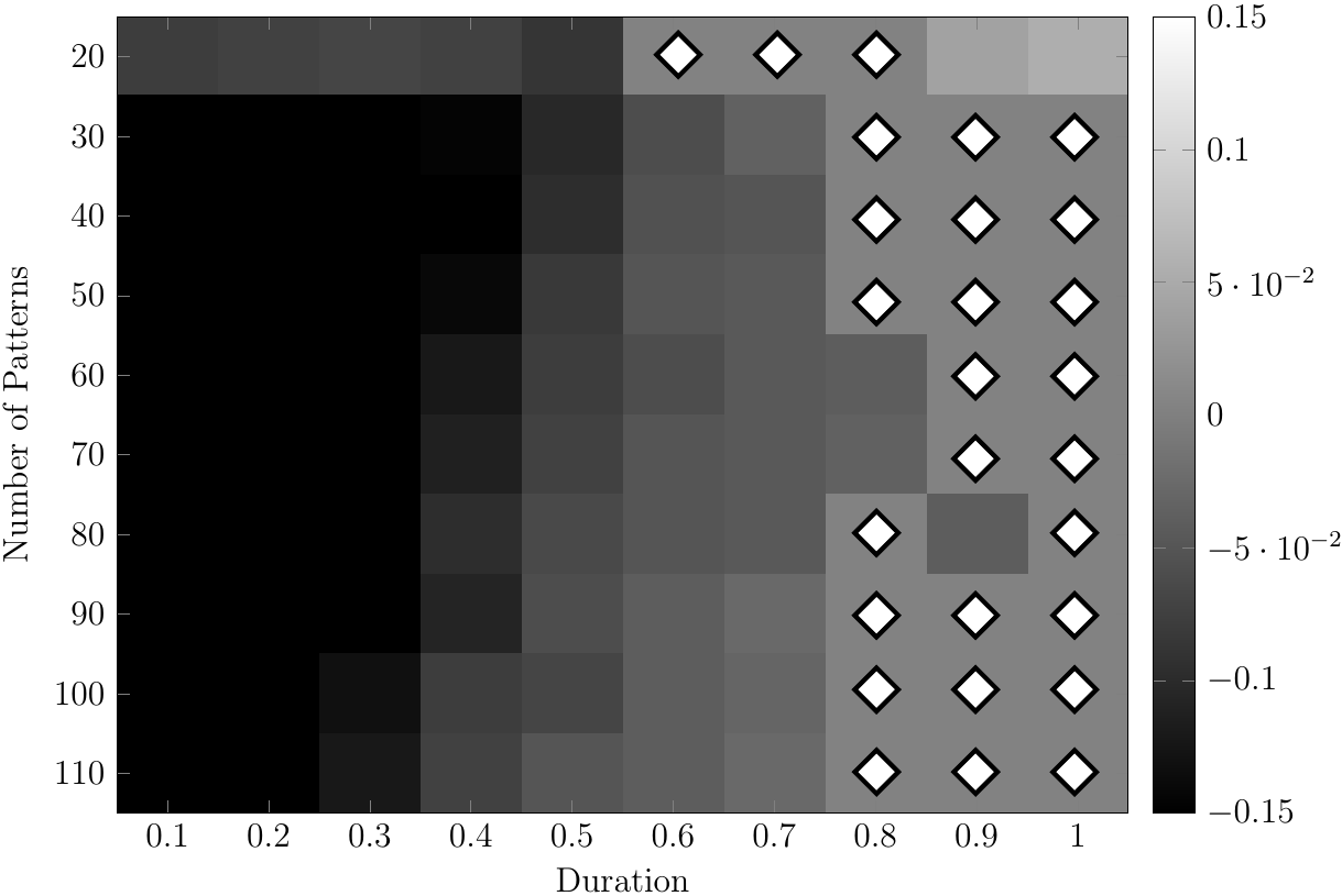
Fig. 2: Left: Mean distances $dist$ obtained with the Multi-SSSA. Middle: Difference between the mean distances obtained with the Multi-SSSA and those obtained with the LARS. Right: Difference between the mean distances obtained with the Multi-SSSA and those obtained with the Group-LASSO solver. The white diamonds correspond to non-significant differences between the means distances.

Compared to the OMP and the LARS, our method obtains same results as them when only few atoms are active at the same time. It happens in our artificial signals when only few patterns have been used to create decomposition matrices and/or when the pattern durations are small. On the contrary, when many atoms are active simultaneously, the OMP and LARS are outperformed by the above algorithm which use inter-signal prior information to find better decompositions.
Compared to the SOMP and the group-LASSO solver, results depend more on the duration of patterns. When patterns are long and not too numerous, theirs performances is similar to the fused-LASSO one. The SOMP is outperformed in all other cases. On the contrary, the group-LASSO solver is outperformed only when patterns have short/medium durations.

5 Relation to prior works

The simultaneous sparse approximation of multi-dimensional signals has been widely studied during these last years [13] and numerous methods developed [14, 15, 16, 17, 4]. More recently, the concept of structured sparsity has considered the encoding of priors in complex regularizations [18, 19]. Our problem belongs to this last category with a regularization combining a classical sparsity term and a Total Variation one. This second term has been studied intensively for image denoising as in the ROF model [20, 21].
The combination of these terms has been introduced as the fused-LASSO [5]. Despite its convexity, the two $\ell_{1}$ non-differentiable terms make it difficult to solve. The initial paper [5] transforms it to a quadratic problem and uses standard optimization tools (SQOPT). Increasing the number of variables, this approach can not deal with large-scale problems. A path algorithm has been developed but is limited to the particular case of the fused-LASSO signal approximator [22]. More recently, scalable approaches based on proximal sub-gradient methods [23], ADMM [24] and split Bregman iterations [6] have been proposed for the general fused-LASSO.
To the best of our knowledge, the multi-dimensional fused-LASSO in the context of overcomplete representations has never been studied. The closest work we found considers a problem of multi-task regression [7]. The final paper had been published under a different title [25] and proposes a new method based on the approximation of the fused-LASSO TV penalty by a smooth convex function as described in [26].

6 Conclusion and Perspectives

This paper has shown the efficiency of the proposed Multi-SSSA based on a split Bregman approach, in order to achieve the sparse structured approximation of multi-dimensional signals, under general conditions. Specifically, the extensive validation has considered different regimes in terms of the signal complexity and dynamicity (number of patterns simultaneously involved and average duration thereof), and it has established a relative competence map of the proposed Multi-SSSA approach comparatively to the state of the art. Further work will apply the approach to the motivating application domain, namely the representation of EEG signals.

References

- [1] D.L. Donoho, “Compressed sensing,” Information Theory, IEEE Trans. on, vol. 52, no. 4, pp. 1289–1306, 2006.
- [2] J. Mairal, M. Elad, and G. Sapiro, “Sparse representation for color image restoration,” Image Processing, IEEE Trans. on, vol. 17, no. 1, pp. 53–69, 2008.
- [3] I. Tošić and P. Frossard, “Dictionary learning,” Signal Processing Magazine, IEEE, vol. 28, no. 2, pp. 27–38, 2011.
- [4] A. Rakotomamonjy, “Surveying and comparing simultaneous sparse approximation (or group-Lasso) algorithms,” Signal Processing, vol. 91, no. 7, pp. 1505–1526, 2011.
- [5] R. Tibshirani, M. Saunders, S. Rosset, J. Zhu, and K. Knight, “Sparsity and smoothness via the fused Lasso,” Journal of the Royal Statistical Society: Series B (Statistical Methodology), vol. 67, no. 1, pp. 91–108, 2005.
- [6] G.B. Ye and X. Xie, “Split Bregman method for large scale fused Lasso,” Computational Statistics & Data Analysis, vol. 55, no. 4, pp. 1552–1569, 2011.
- [7] X. Chen, S. Kim, Q. Lin, J.G. Carbonell, and E.P. Xing, “Graph-structured multi-task regression and an efficient optimization method for general fused Lasso,” arXiv preprint arXiv:1005.3579, 2010.
- [8] T. Goldstein and S. Osher, “The split Bregman method for regularized problems,” SIAM Journal on Imaging Sciences, vol. 2, no. 2, pp. 323–343, 2009.
- [9] C. Wu and X.C. Tai, “Augmented Lagrangian method, dual methods, and split Bregman iteration for ROF, vectorial TV, and high order models,” SIAM Journal on Imaging Sciences, vol. 3, no. 3, pp. 300–339, 2010.
- [10] Y.C. Pati, R. Rezaiifar, and P.S. Krishnaprasad, “Orthogonal matching pursuit: Recursive function approximation with applications to wavelet decomposition,” in Signals, Systems and Computers, 1993. Conf. Record of The Twenty-Seventh Asilomar Conf. on. IEEE, 1993, pp. 40–44.
- [11] B. Efron, T. Hastie, I. Johnstone, and R. Tibshirani, “Least angle regression,” The Annals of statistics, vol. 32, no. 2, pp. 407–499, 2004.
- [12] A. Beck and M. Teboulle, “A fast iterative shrinkage-thresholding algorithm for linear inverse problems,” SIAM Journal on Imaging Sciences, vol. 2, no. 1, pp. 183–202, 2009.
- [13] J. Chen and X. Huo, “Theoretical results on sparse representations of multiple-measurement vectors,” Signal Processing, IEEE Trans. on, vol. 54, no. 12, pp. 4634–4643, 2006.
- [14] J.A. Tropp, A.C. Gilbert, and M.J. Strauss, “Algorithms for simultaneous sparse approximation. Part I: Greedy pursuit,” Signal Processing, vol. 86, no. 3, pp. 572–588, 2006.
- [15] J.A. Tropp, “Algorithms for simultaneous sparse approximation. Part II: Convex relaxation,” Signal Processing, vol. 86, no. 3, pp. 589–602, 2006.
- [16] R. Gribonval, H. Rauhut, K. Schnass, and P. Vandergheynst, “Atoms of all channels, unite! Average case analysis of multi-channel sparse recovery using greedy algorithms,” Journal of Fourier analysis and Applications, vol. 14, no. 5, pp. 655–687, 2008.
- [17] S.F. Cotter, B.D. Rao, K. Engan, and K. Kreutz-Delgado, “Sparse solutions to linear inverse problems with multiple measurement vectors,” Signal Processing, IEEE Trans. on, vol. 53, no. 7, pp. 2477–2488, 2005.
- [18] J. Huang, T. Zhang, and D. Metaxas, “Learning with structured sparsity,” Journal of Machine Learning Research, vol. 12, pp. 3371–3412, 2011.
- [19] R. Jenatton, J.Y. Audibert, and F. Bach, “Structured variable selection with sparsity-inducing norms,” Journal of Machine Learning Research, vol. 12, pp. 2777–2824, 2011.
- [20] L.I. Rudin, S. Osher, and E. Fatemi, “Nonlinear total variation based noise removal algorithms,” Physica D: Nonlinear Phenomena, vol. 60, no. 1-4, pp. 259–268, 1992.
- [21] J. Darbon and M. Sigelle, “A fast and exact algorithm for total variation minimization,” in Pattern recognition and image analysis, 2005, vol. 3522 of Lecture Notes in Computer Science, pp. 351–359.
- [22] H. Hoefling, “A path algorithm for the fused Lasso signal approximator,” Journal of Computational and Graphical Statistics, vol. 19, no. 4, pp. 984–1006, 2010.
- [23] J. Liu, L. Yuan, and J. Ye, “An efficient algorithm for a class of fused Lasso problems,” in Proc. 16th ACM SIGKDD Int. Conf. on Knowledge Discovery and Data Mining. ACM, 2010, pp. 323–332.
- [24] B. Wahlberg, S. Boyd, M. Annergren, and Y. Wang, “An ADMM algorithm for a class of total variation regularized estimation problems,” arXiv preprint arXiv:1203.1828, 2012.
- [25] X. Chen, Q. Lin, S. Kim, J.G. Carbonell, and E.P. Xing, “Smoothing proximal gradient method for general structured sparse regression,” The Annals of Applied Statistics, vol. 6, no. 2, pp. 719–752, 2012.
- [26] Y. Nesterov, “Smooth minimization of non-smooth functions,” Mathematical Programming, vol. 103, no. 1, pp. 127–152, 2005.